





1. Introduction
Understanding and controlling the wetting process is of great importance for a wide range of applications, such as coating, inkjet printing, oil recovery and microfluidic devices (De Gennes Reference De Gennes1985; Bonn et al. Reference Bonn, Eggers, Indekeu, Meunier and Rolley2009). The key issue of wetting phenomena is the quantitative characterization of the three-phase contact line behaviour and contact angle. For a smooth and chemically homogeneous (ideal) solid surface, there is a single equilibrium contact angle, which can be described by the well-known Young's equation. However, real surfaces may have physical roughness and/or chemical heterogeneity, which would result in contact angle hysteresis (CAH) and associated complex contact line dynamics (Wang, Qian & Sheng Reference Wang, Qian and Sheng2008; Savva, Kalliadasis & Pavliotis Reference Savva, Kalliadasis and Pavliotis2010; Savva & Kalliadasis Reference Savva and Kalliadasis2013; Savva, Groves & Kalliadasis Reference Savva, Groves and Kalliadasis2019). An essential understanding has been formed that CAH is related to the existence of multiple equilibrium configurations of the fluid interface induced by the non-uniformity of a solid surface. The energy barriers between stable/metastable equilibrium configurations can trap the system in different states depending on the motion history of the contact line. In this way, the apparent contact angle may take an arbitrary value in the range  $[\theta _R,\theta _A]$, where
 $\theta _R$ and
 $\theta _A$ are the receding and advancing contact angles, respectively.
Due to the importance of CAH in surface engineering, many works have been devoted to the understanding of the fundamental mechanisms of CAH from theoretical (Joanny & De Gennes Reference Joanny and De Gennes1984; Marmur Reference Marmur1994a,Reference Marmurb; Gao & McCarthy Reference Gao and McCarthy2006; Iwamatsu Reference Iwamatsu2006; Xu & Wang Reference Xu and Wang2011; Giacomello, Schimmele & Dietrich Reference Giacomello, Schimmele and Dietrich2016; Hatipogullari et al. Reference Hatipogullari, Wylock, Pradas, Kalliadasis and Colinet2019), numerical (Crassous & Charlaix Reference Crassous and Charlaix1994; Brandon & Marmur Reference Brandon and Marmur1996; Brandon et al. Reference Brandon, Haimovich, Yeger and Marmur2003; Kusumaatmaja & Yeomans Reference Kusumaatmaja and Yeomans2007; David & Neumann Reference David and Neumann2010) and experimental (Di Meglio & Quéré Reference Di Meglio and Quéré1990; Di Meglio Reference Di Meglio1992; Ramos et al. Reference Ramos, Charlaix, Benyagoub and Toulemonde2003; Priest, Sedev & Ralston Reference Priest, Sedev and Ralston2007; Reyssat & Quéré Reference Reyssat and Quéré2009; Delmas, Monthioux & Ondarçuhu Reference Delmas, Monthioux and Ondarçuhu2011; Priest, Sedev & Ralston Reference Priest, Sedev and Ralston2013; Guan et al. Reference Guan, Wang, Charlaix and Tong2016; Perrin et al. Reference Perrin, Lhermerout, Davitt, Rolley and Andreotti2016; Wang et al. Reference Wang, Guo, Chen and Tong2016; Lhermerout & Davitt Reference Lhermerout and Davitt2018; Fuentes et al. Reference Fuentes, Hatipogullari, Van Hoof, Vitry, Dehaeck, Du Bois, Lambert, Colinet, Seveno and Van Vuure2019; Guan, Charlaix & Tong Reference Guan, Charlaix and Tong2020) perspectives. For instance, Marmur and others investigated the CAH of a sessile droplet placed on a periodically heterogeneous surface (Marmur Reference Marmur1994a; Brandon & Marmur Reference Brandon and Marmur1996; Montes Ruiz-Cabello et al. Reference Montes Ruiz-Cabello, Rodríguez-Valverde, Marmur and Cabrerizo-Vílchez2011). Kusumaatmaja & Yeomans (Reference Kusumaatmaja and Yeomans2007) numerically investigated the CAH on chemically patterned and superhydrophobic surfaces as the droplet volume was quasi-statically increased or decreased. Systematic experiments have been carried out for studying CAH on heterogeneous surfaces with a random array of defects from the microscale (Di Meglio Reference Di Meglio1992; Nadkarni & Garoff Reference Nadkarni and Garoff1992; Priest et al. Reference Priest, Sedev and Ralston2007; Reyssat & Quéré Reference Reyssat and Quéré2009; Priest et al. Reference Priest, Sedev and Ralston2013; Fuentes et al. Reference Fuentes, Hatipogullari, Van Hoof, Vitry, Dehaeck, Du Bois, Lambert, Colinet, Seveno and Van Vuure2019) to the nanoscale (Ramos et al. Reference Ramos, Charlaix, Benyagoub and Toulemonde2003; Delmas et al. Reference Delmas, Monthioux and Ondarçuhu2011; Lhermerout & Davitt Reference Lhermerout and Davitt2018). Recently, a newly developed atomic-force-microscope measurement method (Delmas et al. Reference Delmas, Monthioux and Ondarçuhu2011; Guan et al. Reference Guan, Wang, Charlaix and Tong2016, Reference Guan, Charlaix and Tong2020; Wang et al. Reference Wang, Guo, Chen and Tong2016) was used to study the CAH on non-ideal long-fibre surfaces. A strong asymmetric speed dependence (Guan et al. Reference Guan, Wang, Charlaix and Tong2016) as well as state and rate dependencies (Guan et al. Reference Guan, Charlaix and Tong2020) of contact line dynamics were reported.
Although considerable progress has been made in understanding CAH, there are still several critical open questions. In experiments, the pinning–depinning behaviour of the contact line is usually accompanied by the occurrence of CAH (Priest et al. Reference Priest, Sedev and Ralston2013). Pinning is often considered to be responsible for CAH (Delmas et al. Reference Delmas, Monthioux and Ondarçuhu2011), or free energy barriers that cause CAH are used to explain the pinning–depinning mechanism (Orejon, Sefiane & Shanahan Reference Orejon, Sefiane and Shanahan2011; Zhang, Huang & Lu Reference Zhang, Huang and Lu2019). However, recent molecular dynamics simulations show that microscopic contact line pinning is a slowdown of contact line dynamics under the control of capillary force balance, and it may not be related to free energy barriers (Zhang, Müller-Plathe & Leroy Reference Zhang, Müller-Plathe and Leroy2015). Therefore, the relationship between microscopic pinning–depinning of the contact line and CAH has to be further explored.
It has been found that the typical gas–liquid interface (GLI) length  $L_i$ (GLI area for three-dimensional (3-D) cases) is an important physical parameter determining the hysteresis behaviour. The size effect of the GLI on CAH has attracted much attention (Quéré Reference Quéré2008; Ozcelik, Satiroglu & Barisik Reference Ozcelik, Satiroglu and Barisik2020). In previous studies, a sessile droplet system (see figure 1a) was usually chosen to study CAH by increasing or decreasing the droplet volume quasi-statically (Marmur Reference Marmur1994a; Brandon & Marmur Reference Brandon and Marmur1996; Kusumaatmaja & Yeomans Reference Kusumaatmaja and Yeomans2007; Pradas et al. Reference Pradas, Savva, Benziger, Kevrekidis and Kalliadasis2016). In this circumstance, the deformation of the GLI depends not only on the properties of the solid surface but also on the droplet volume. As a result, irregular oscillatory curves would be obtained to describe the evolution of receding and advancing contact angles (Marmur Reference Marmur1994a), which is not conducive to the statistical analysis of CAH. Recently, Hatipogullari et al. (Reference Hatipogullari, Wylock, Pradas, Kalliadasis and Colinet2019) and Xu & Wang (Reference Xu and Wang2011) studied CAH using a chemically heterogeneous microchannel (see figure 1b). The advantage of choosing this system is that the typical GLI length (approximately equal to the microchannel width) does not vary with liquid volume. Qualitatively, Xu & Wang (Reference Xu and Wang2011) found that on a periodically patterned microchannel, for a given microchannel width, the receding and advancing contact angles fluctuate periodically as liquid volume changes. Hatipogullari et al. (Reference Hatipogullari, Wylock, Pradas, Kalliadasis and Colinet2019) extended the graphical force balance approach proposed by Joanny & De Gennes (Reference Joanny and De Gennes1984) to two-dimensional (2-D) microchannel systems. For the size effect, they qualitatively found increasing microchannel width brings the system from a subthreshold regime, to a stick–slip-dominated regime and finally to a regime with a quasi-constant advancing and receding angle. However, there is still a lack of quantitative insight into the effect of the typical GLI length on hysteresis behaviour.
Schematic diagrams of (a) a 2-D sessile droplet placed on a chemically heterogeneous substrate, (b) a 2-D droplet and (c) a 3-D droplet confined in chemically heterogeneous microchannels. Here  $x_1$ and
 $x_2$ represent the locations of the droplet's contact points, and the corresponding apparent contact angles are
 $\theta _{a1}$ and
 $\theta _{a2}$, respectively. Parameter
 $R$ is the base radius. The microchannel width is
 $b$ and the spatial period of chemical heterogeneity is
 $\beta$. (d,e) Two typical 2-D surface wettability distributions.

Another unresolved key problem is the complete theoretical modelling of the relationship between CAH and the properties of a substrate's disorder. For individual-effect-dominated hysteresis (IDH), i.e. contact line jumping is only affected by individual defects, Joanny & De Gennes (Reference Joanny and De Gennes1984) proposed a scaling law by considering the mechanical balance of capillary force exerted by the defects (i.e. defect force) and the elastic restoring force due to the deformation of the contact line:
 \begin{equation} H\propto \phi F_{d,max}^2. \end{equation}
Here  $\phi$ is the number of defects per unit area (defect density),
 $F_{d,max}$ the maximum defect force and
 $H$ the value of CAH. Subsequently, this scaling law was verified by experiments (Di Meglio Reference Di Meglio1992; Ramos et al. Reference Ramos, Charlaix, Benyagoub and Toulemonde2003; Delmas et al. Reference Delmas, Monthioux and Ondarçuhu2011; Lhermerout & Davitt Reference Lhermerout and Davitt2018). Hatipogullari et al. (Reference Hatipogullari, Wylock, Pradas, Kalliadasis and Colinet2019) performed theoretical analysis on the threshold value of wettability gradients inducing hysteresis and the scaling law for the IDH mode (1.1) by using 2-D microchannels. However, if contact line jumping is affected by two neighbouring defects, it is referred to as collective-effect-dominated hysteresis (CDH). The contact line behaviour in CDH may significantly differ from that in IDH (Di Meglio & Quéré Reference Di Meglio and Quéré1990; Di Meglio Reference Di Meglio1992; Reyssat & Quéré Reference Reyssat and Quéré2009). As far as we know, there is no explicit theoretical explanation for CAH under the collective effect (Quéré Reference Quéré2008; Bonn et al. Reference Bonn, Eggers, Indekeu, Meunier and Rolley2009). This severely limits the further understanding of CAH and even wetting phenomena.
The present work is committed to exploring the open issues discussed above. To this end, we systematically investigate the quasi-static CAH in a chemically heterogeneous microchannel by theoretical analysis and numerical simulations based on a diffuse-interface method. We focus on the size effect and the related scaling laws. It is noticed that conclusions coming from chemically heterogeneous microchannels are also applicable to microchannels with physical roughness (Joanny & De Gennes Reference Joanny and De Gennes1984). Here in our study, we mainly investigate 2-D cases and then check whether the conclusions are applicable to 3-D cases.
The remainder of this paper is organized as follows. The problem statement and mathematical formulation are presented in § 2. The numerical method is described in § 3. Detailed results for 2-D and 3-D cases are discussed in §§ 4 and 5, respectively. Finally, conclusions are presented in § 6.
2. Problem statement and mathematical formulation
2.1. Physical problem
Here we consider the GLI motion in a microchannel with a width of  $b$. The upper and lower walls of the microchannel are smooth, rigid and flat, but have the same periodic chemical heterogeneity (as shown in figure 1b,c). The spatial period of surface heterogeneity is
 $\beta$, which is the same in both horizontal directions for 3-D cases. The chemical heterogeneity is characterized by a spatially dependent intrinsic contact angle
 $\theta _i$ that is defined by Young's equation. Two typical 2-D surface wettability distributions are shown in figures 1(d) and 1(e), respectively. The droplet volume increases or decreases by quasi-static condensation or evaporation, which drives the GLI and contact line movements. For 2-D cases, sharp-edged defects (so-called mesa defects; see figure 1d) are mainly considered because they can cause a variety of contact line dynamics behaviour, and have been widely adopted in previous studies (Wang et al. Reference Wang, Qian and Sheng2008; Zhang et al. Reference Zhang, Müller-Plathe and Leroy2015). For 3-D microchannels, an array of circular defects is regularly distributed on the surface. In the current work, gravity is not considered.
2.2. Mathematical formulation
For the 2-D cases, although asymmetric phase transitions can also exist, we only consider the symmetric regimes (left–right and top–bottom). Here the GLI is approximated by a circular arc. Then the theoretical description of the system can be performed. Because the phase transitions on the left- and right-hand sides are symmetric, the GLI and contact line motions on both sides are identical. Therefore we have  $\theta _{a1}=\theta _{a2}=\theta _{a}$ and
 $x_2=-x_1$. Here
 $x_1$ and
 $x_2$ represent the locations of the droplet's contact points, and the corresponding apparent contact angles are
 $\theta _{a1}$ and
 $\theta _{a2}$, respectively. Defining base radius as
 $R=(x_2-x_1)/2$, we have the volume of liquid (it is actually the cross-sectional area for 2-D cases) given by
 \begin{equation} V(R)=2Rb+b^2\frac{2\theta_a-{\rm \pi}+\sin 2\theta_a}{4\cos ^2\theta_a}. \end{equation}
In order to analyse the stability of the system, the interfacial free energy is calculated. For a fixed droplet volume, the interfacial energy per unit length of the contact line can be determined from the length of the GLI and the solid–liquid interface by
 \begin{equation} E(R)=\gamma b \left(\frac{{\rm \pi}-2\theta_a}{\cos \theta_a}\right)-4\gamma\int_{0}^{R} \cos \theta_i(x)\,{\rm d} x, \end{equation}
where  $\gamma$ is the gas–liquid surface tension. Obviously, the system is at equilibrium at the stationary points/extrema of the free energy function (i.e.
 $\partial E/\partial R=0$).
Here we choose  $\beta$ as the characteristic length to normalize the system, and the corresponding dimensionless variables are given by
 \begin{equation} b^*=\frac{b}{\beta},\quad R^*=\frac{R}{\beta},\quad V^*=\frac{V}{\beta^2},\quad E^*=\frac{E}{\beta\gamma}. \end{equation}
For simplicity, we will drop the asterisk notation in the remainder of the paper.
3. Numerical method
In recent years, the lattice Boltzmann method (LBM) has been developed into an effective and powerful computational fluid dynamics technique. It has been widely used in modelling complex multiphase flows including boiling (Chang, Huang & Lu Reference Chang, Huang and Lu2017; Chang et al. Reference Chang, Huang, Cheng and Lu2019), droplet evaporation and condensation (Ledesma-Aguilar, Vella & Yeomans Reference Ledesma-Aguilar, Vella and Yeomans2014; Hessling, Xie & Harting Reference Hessling, Xie and Harting2017) and the moving contact line problem (Kusumaatmaja, Hemingway & Fielding Reference Kusumaatmaja, Hemingway and Fielding2016). The multiphase LBM, as a diffuse-interface model, can automatically capture the GLI by incorporating two-phase interactions.
Here we implement the multicomponent multiphase (MCMP) pseudopotential lattice Boltzmann model proposed by Shan & Chen (Reference Shan and Chen1993) in two and three dimensions. Considering the flow system composed of two components, there are two distribution functions and each function describes the evolution of a component. Each distribution function satisfies the following lattice Boltzmann equation:
 \begin{equation} f_i^{\sigma} ( {\boldsymbol{x} + \boldsymbol{e}_i \Delta t,t + \Delta t} ) = f_i^{\sigma} ( {\boldsymbol{x},t} ) - \frac{\Delta t}{\tau_{\sigma} }[ {f_i^{\sigma} ( {\boldsymbol{x},t} ) - f_i^{\sigma,eq} ( {\boldsymbol{x},t} )}], \end{equation}
where  $f_i^{\sigma } ( {\boldsymbol {x},t} )$ is the density distribution function for component
 $\sigma$ and
 $\boldsymbol {e}_i$ (
 $i=0,1,\ldots 8$ for 2-D cases and
 $i=0,1,\ldots 18$ for 3-D cases) are the discrete velocities. Function
 $f_i^{\sigma,eq} ( {\boldsymbol {x},t} )$ is the equilibrium distribution function. The relaxation time
 $\tau _{\sigma }$ is related to the kinematic viscosity as
 $\nu _{\sigma } = c_s^2( {\tau _{\sigma } - 0.5\Delta t} )$, where sound speed
 $c_s={c}/{\sqrt {3}}$ and
 $c= {\Delta x}/{\Delta t}$. The grid spacing
 $\Delta x=1$ and the time step
 $\Delta t=1$. In our simulations,
 $\tau _{\sigma }=1$, i.e.
 $\tau _1=\tau _2=1$. Note that in the LBM, the values of physical variables are given in lattice units. For a specific component,
 $\rho ^{maj}$ and
 $\rho ^{min}$ are the component densities at the two sides of the miscibility gap (the miscibility gap being symmetric in the model). Before simulations, we have to specify the density of the whole fluid
 $\rho ^{maj}+\rho ^{min}$, which is a constant in the whole computational domain. Here the value of
 $\rho ^{maj}+\rho ^{min}$ is chosen a priori as
 $0.736$.
Using the Chapman–Enskog expansion, the lattice Boltzmann equation recovers the macroscopic governing equations, i.e. Navier–Stokes equations (Chai & Zhao Reference Chai and Zhao2012):
 $$\begin{gather} \frac{\partial \rho}{\partial t} +\boldsymbol{\nabla}\boldsymbol{\cdot}(\rho \boldsymbol{u}) =0, \end{gather}$$
 $$\begin{gather}\frac{\partial (\rho\boldsymbol{u})}{\partial t} +\boldsymbol{\nabla}\boldsymbol{\cdot}(\rho \boldsymbol{uu}) ={-}\boldsymbol{\nabla} p+ \boldsymbol{\nabla}\boldsymbol{\cdot}[\rho\nu(\boldsymbol{\nabla}\boldsymbol{u}+ \boldsymbol{\nabla}\boldsymbol{u}^T )]+\boldsymbol{F}, \end{gather}$$
where  $\rho$,
 $\boldsymbol {u}$,
 $p$ and
 $\boldsymbol {F}$ are the mixture density, velocity, pressure and force term, respectively. Specifically,
 $\rho =\sum _{\sigma } {\rho _{\sigma } }$ and
 $\boldsymbol {u}=({1}/{\rho })(\sum _{\sigma } \sum _i f_i^{\sigma }\boldsymbol {e}_i+({1}/{2})\sum _{\sigma }\boldsymbol {F}_{\sigma }\Delta t)$ (Shan & Doolen Reference Shan and Doolen1995). Here
 $\rho _{\sigma }$ is the density of component
 $\sigma$ and
 $\boldsymbol {F}_{\sigma }$ is the force acting on component
 $\sigma$. The mixture viscosity
 $\nu =\nu _1=\nu _2$ since
 $\tau _1$ and
 $\tau _2$ are identical. It should be noted that what is solved by the two-component MCMP pseudopotential lattice Boltzmann model is actually the liquid–liquid problem rather than the liquid–vapour problem. In other words, the droplet in the microchannel undergoes a dissolution/precipitation process in the surrounding liquid, which shares a common mechanism with the evaporation/condensation process of the droplet in the quasi-static limit (Xie & Harting Reference Xie and Harting2019). In this mechanism, the mass change rate of the droplet is dominated by the diffusion of the droplet into the surrounding environment driven by the concentration or density gradient of droplet component in the surrounding fluid and the ambient pressure remains constant. Mathematically, these two processes are both dominated by the unsteady diffusion equation, known as Fick's second law. Since the two-component lattice Boltzmann model rather than the single-component two-phase lattice Boltzmann model (liquid–vapour model) can keep the ambient pressure constant when introducing the density gradient, we choose the former to simulate the droplet phase transitions in a microchannel.
To simulate droplet evaporation and condensation in a microchannel, the following dimensionless governing parameters are defined: the Reynolds number  $Re=U_c L/\nu _1$, the capillary number
 $Ca=\rho ^{maj}\nu _1 U_c/\gamma$, the Péclet number
 $Pe=U_c L/D_{1}$ and the Cahn number
 $Cn=\lambda /L$. Here,
 $L$,
 $U_c$ and
 $\lambda$ are the characteristic length, velocity and interfacial thickness, respectively. Parameter
 $D_{1}$ is the diffusivity of fluid 1. More basic introductions for the LBM and the detailed parameter settings are described in Appendices A.1 and A.2, respectively. The parameter settings are also introduced briefly in the following.
For a specific flow problem, simulation parameters, such as  $D_1$,
 $\gamma$ and
 $\lambda$, can be determined by specified dimensionless parameters. Suppose
 $\tau _1$ is specified, then we have the viscosity of component 1
 $\nu _1$. From the definition of
 $Re$ and the specified value of
 $L$, we can obtain
 $U_c$. According to the definition of
 $Pe$, we can determine the diffusivity
 $D_1$. For specific
 $\tau _1$ and
 $\tau _2$,
 $D_1$,
 $\sigma$ and
 $\lambda$ are functions of
 $G$. In addition, if
 $\rho ^{maj}+\rho ^{min}$ is given a priori,
 $\rho ^{maj}$ and
 $\rho ^{min}$ are also functions of
 $G$. Through
 $D_1$, the correct choice of cohesion force parameter
 $G$ can be obtained (here
 $G=3.6$), and then
 $\gamma$,
 $\lambda$,
 $\rho ^{maj}$ and
 $\rho ^{min}$ can all be determined (see Appendix A.2).
To impose the wetting condition on the solid surface, the surface energy formulation from the phase-field method (Fakhari & Bolster Reference Fakhari and Bolster2017) is extended to the MCMP pseudopotential lattice Boltzmann framework. This formula is able to handle complex geometric boundaries and determine the contact angle a priori. For the details of extending wetting boundary conditions to the MCMP pseudopotential LBM, refer to Appendix A.3. The numerical method is well validated in Appendix B.
Discretization errors in the computation of the cohesion force cause spurious currents around the interface. The absolute magnitude of spurious currents may be of the order  $0.01$ in our simulations. However, the spurious currents do not affect the evolution of the interface and the behaviour of the contact line under quasi-static circumstances. The evaporation and condensation simulations in Appendix B confirm this point.
4. Two-dimensional results and discussion
4.1. Contact line dynamics
We consider microchannel surfaces composed of alternating equal-width stripes of different wettabilities as shown in figure 1(d), which can be described by
 \begin{equation} \cos \theta_i(x)=\cos \theta_0+\frac{\varepsilon}{2}\tanh [M\cos (2{\rm \pi} x/\beta)], \end{equation}
where  $M\to \infty$. This corresponds to the cases with a discontinuous wetting property at the junction of two types of stripes. Angle
 $\theta _0$ is the reference contact angle and
 $\varepsilon$ controls the strength of the chemical heterogeneity. Through the theoretical analysis described in § 2.2 combined with the local Cassie–Baxter (LCB) equation (Zhang et al. Reference Zhang, Müller-Plathe and Leroy2015), we can obtain all equilibrium configurations at different droplet volumes as shown in figure 2(a). Here the LCB equation is introduced to determine
 $\theta _a$ by
 $R$ when the contact line is located at the junction of two types of stripes, which is expressed as
 \begin{equation} \cos \theta_a =f_A\cos \theta_{Ai}+f_B\cos \theta_{Bi}, \end{equation}
where  $\theta _{Ai}$ and
 $\theta _{Bi}$ are the intrinsic contact angles of stripes A and B, respectively. Also,
 $f_A=l_A/\lambda$ and
 $f_B=l_B/\lambda$ are the thickness ratios;
 $l_A$ and
 $l_B$ are the thicknesses of the diffused contact line occupied by stripes A and B, respectively (see figure 3). Using the LCB equation, when
 $R$ and
 $\lambda$ are known,
 $f_A$ and
 $f_B$ can be calculated, and then
 $\theta _a$ is obtained. Therefore, figure 2(a) is generated using (2.1) and the LCB equation. Since
 $Cn$ controls
 $\lambda$, when we plot figure 2(a),
 $Cn$ is a relevant parameter.
(a) Stable/metastable and unstable equilibrium configurations given by (2.1) for different droplet volumes. Here  $\theta _0=90^\circ$,
 $\varepsilon =1.0$,
 $b=10$ and
 $Cn=0.108$. (b) Free energy as a function of the apparent contact angle for
 $V/b=4.6$ (the left-hand dashed line in a), where
 $\theta _m$ is the most stable apparent contact angle. The black solid lines in the five insets show the fluid interfaces on the left-hand side of the droplet at equilibrium states. In each inset, due to symmetry, only half of the droplet is shown and the vertical dash-dotted line is the symmetric axis of the droplet. The aspect ratio is not to scale in the insets due to space limitation. If they are plotted according to
 $b=10$ instead of
 $b\approx 2$, the droplet volumes are identical.

Schematic diagram of the calculation of apparent contact angle  $\theta _a$ using the LCB equation.

It can be seen from figure 2(a) that for a given value of droplet volume, there is an odd number of equilibrium configurations. They represent the stable/metastable and unstable equilibrium states of the system, alternately corresponding to the minima and maxima of the free energy curve (see figure 2b). The outermost equilibrium configurations are stable or metastable (e.g. points A and E in figure 2b). Two adjacent stable/metastable states are separated by an unstable state with a free energy barrier (e.g. points A and C are separated by point B in figure 2b). Because of multiple equilibrium states, there are different motion trajectories of contact line as the droplet evaporates or condenses.
It is also noticed that the almost horizontal segments in figure 2(a) have non-zero slopes. Actually, due to our diffuse-interface model, even at the pinning stage,  $R$ is not a constant and may change slightly. More specifically, the change depends on
 $Cn$. When
 $Cn\to 0$ (corresponding to the macro-circumstance), since
 $M\to \infty$, the slope of the line segment in the pinning stage is zero.
In order to get more details of the contact line behaviour, we carry out several simulations of quasi-static evaporation/condensation of a droplet in the chemically patterned microchannel. The computational domain size is  $20\times b$. In our simulations,
 $\beta =50\Delta x$, so the mesh size is
 $1000\times 50b$. Initially a rectangular droplet containing fluid 1 with
 $\rho _1=\rho ^{maj}$ and fluid 2 with
 $\rho _2=\rho ^{min}$ is placed in the middle of the 2-D microchannel, and the surrounding volume consists of fluid 2
 $\rho _2=\rho ^{maj}$ and fluid 1
 $\rho _1=\rho ^{min}$. To drive the phase transition, a density gradient is set in the surrounding volume. For the upper and lower walls, we set the wetting condition through (A13) and set the no-slip condition. For detailed settings of boundary conditions, see Appendix A.3. Here the governing parameters are
 $Re=0.003$,
 $Ca=0.000025$,
 $Pe=0.0042$ and
 $Cn=0.108$. Values of
 $\theta _0$ and
 $\varepsilon$ are chosen as
 $90^\circ$ and
 $1.0$, respectively.
The droplet's base radius  $R$, the apparent contact angle
 $\theta _a$ and the interfacial free energy
 $E$ as functions of
 $V/b$ for the cases of
 $b= 1.6$,
 $4$ and
 $10$ are plotted in figure 4. The results of condensation and evaporation present the advancing and receding paths of the contact line, respectively. The equilibrium configurations obtained from the theory are also shown in the figure for comparison. One can see that the advancing and receding paths follow the outermost equilibrium configurations of the system since there is no additional energy to overcome the energy barriers. Specifically, the advancing path corresponds to the outermost equilibrium configuration with a higher apparent contact angle, and the receding path corresponds to that with a lower apparent contact angle. It is worth noting that there are some critical points (e.g. points O and P in figure 4d–f) on the motion paths of the contact line. Saddle-node bifurcations occur at these points. Meanwhile, the outermost metastable equilibrium point coincides with the adjacent unstable equilibrium point (e.g. point O in figure 4d–f) and disappears immediately. Subsequently, the contact line suddenly jumps to the nearest metastable point with lower surface energy. The excess surface energy is dissipated through capillary waves during the rapid jump (see figure 4c, f,i). It should be noted that similar effects of bifurcation diagrams have also been reported in a recent contribution on sessile droplets (Groves & Savva Reference Groves and Savva2021). In general, our simulation accurately reproduces the CAH and complex contact line dynamics predicted by the theory.
Comparison of CAH behaviour simulated by the LBM with that predicted by theory for cases with different  $b$. (a,d,g) Droplet base radius
 $R$, (b,e,h) apparent contact angle
 $\theta _a$ and (c, f,i) system free energy
 $E$ as functions of droplet volume. Cases of (a–c)
 $b=1.6$, (d–f)
 $b=4$ and (g–i)
 $b=10$.

In addition to jumping, other contact line behaviours, such as pinning–depinning and slip, depend entirely on the outermost equilibrium configuration varying with  $V$, which is due to the surface chemistry. In particular, pinning–depinning occurs at the junction of two types of stripes where the wettability gradient direction is consistent with the fluid density gradient direction near the contact line. Pinning is a slowdown of the contact line dynamics dominated by the local Young's equation. When a contact line, which undergoes a slowdown stage and appears to be pinned macroscopically, completely transitions to a homogeneous part of heterogeneity, the contact line accelerates thus triggering a depinning event. All this implies that microscopic contact line pinning is not directly related to CAH, which further supports the recent result of Pradas et al. (Reference Pradas, Savva, Benziger, Kevrekidis and Kalliadasis2016).
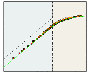
The trajectories followed by apparent contact angle are shown in figure 4(b,e,h). They are two periodic fluctuating curves as observed qualitatively in experiments (Priest et al. Reference Priest, Sedev and Ralston2013; Wang et al. Reference Wang, Guo, Chen and Tong2016). The amplitude of the curves is constant, and the period  $\Delta V=2b$. One can also see that the microchannel width has a significant effect on the contact angle curves. First, when the width is small with
 $b=1.6$, the contact line undergoes a slip–jump–slip–stick movement pattern (figure 5a). During the slip stage, the apparent contact angle remains constant (constant contact angle mode), and during the stick stage, the droplet's base radius remains essentially constant (constant contact radius mode). During the jump process, both the apparent contact angle and the droplet's base radius undergo a sudden change. In figure 5(a), after the jump, the contact line moves to the adjacent stripe and continues to slip for a while until it reaches the next wettability boundary. In the stick process, the trajectories of the advancing and receding fronts coincide (see figure 4b), and the maximum and minimum of advancing and receding contact angles are also the same, which are equal to the inherent contact angles of the hydrophobic and hydrophilic stripes, respectively.
Schematic diagrams for motions of a droplet's left fluid interface near the wall. (a) Slip–jump–slip–stick and (b) slip–jump–stick modes. Here the evaporation process is taken as an example.

On increasing the microchannel width to  $b=4$, the contact line movement transforms into a slip–jump–stick mode (figure 5b). After the jump, the contact line directly reaches the wettability boundary and is stuck. The contact angle curves look jagged and have a smaller amplitude compared with the case of
 $b=1.6$. The advancing and receding paths coincide in a certain segment of the stick stage (see figure 4e). On further increasing the microchannel width to
 $b=10$, the contact line movement mode and the shape of contact angle curves are basically identical to those in the case of
 $b=4$, except that the amplitude of contact angle curves is further reduced, and the advancing and receding paths are completely separated. Assuming
 $b\to \infty$, the amplitude of the contact angle curves will approach
 $0$ and the advancing and receding contact angles remain constant, which are respectively equal to the inherent contact angles of the hydrophobic and hydrophilic stripes. This is consistent with the previous conclusion obtained from surfaces with sinusoidal heterogeneity (Hatipogullari et al. Reference Hatipogullari, Wylock, Pradas, Kalliadasis and Colinet2019).
Our simulations closely follow the branches in figure 4. This is a consequence of the slowness of the changes in volume  $V$. Due to the quasi-static phase transition, the disturbance caused by the changes of
 $V$ is so small that it cannot overcome the free energy barrier. However, if the phase change rate becomes faster, the significant disturbance energy caused by the change of
 $V$ may overcome the free energy barrier and the jump event will occur in advance. In this circumstance, the tracing of the bifurcation curves would not be as precise.
4.2. Equilibrium properties
4.2.1. The number of equilibrium configurations
Since the CAH behaviours obtained from numerical simulation agree well with the theoretical prediction, for convenience, the data obtained from the latter are adopted in the following analysis. Before further quantitatively analysing CAH, we first pay attention to the equilibrium properties of the system. It can be seen from figure 4 that, qualitatively, the number of equilibrium configurations  $N(V)$ increases with
 $b$. This is consistent with the previous conclusion obtained from a sessile droplet system (Brandon et al. Reference Brandon, Haimovich, Yeger and Marmur2003; Wu et al. Reference Wu, Wang, Selzer and Nestler2019). In order to quantitatively explore the influence of
 $b$ on the number of equilibrium configurations, we define a volume-averaged number of equilibrium configurations in the following.
For a microchannel with width  $b$, the number of equilibrium configurations
 $N$ is a function of
 $V$. For example, figure 2(a) shows
 $N=5$ at
 $V=4.6b$, while
 $N=3$ at
 $V=5.5b$ when
 $b=10$. Therefore
 $N$ should change periodically with period
 $\Delta V=2b$. In order to determine how
 $N$ varies with
 $b$, we defined a volume-averaged
 $N$, i.e. the average number of equilibrium configurations in one period
 $\Delta V$:
 \begin{equation} n=\frac{1}{\Delta V}\int_{V_i}^{V_i+\Delta V} N(V)\,{\rm d}V, \end{equation}
where  $V_i$ is an arbitrary value of droplet volume during phase transition. In this way, there is a determined number of equilibrium configurations for cases with a specific
 $b$.
Figure 6(a) shows the number  $n$ as a function of
 $b$ for different heterogeneity strengths
 $\varepsilon$ with
 $\theta _0=90^\circ$. A linear dependence is found. When
 $b\to 0$,
 $n\to 1$. This means that there are no multiple equilibrium configurations and CAH. Besides
 $b$,
 $\theta _0$ as well as
 $\varepsilon$ also affect
 $n$. From the inset of figure 6(a), it can be found that the relationships between
 $n$,
 $\cos \theta _0$ and
 $\varepsilon$ satisfy the quadratic polynomial equation. When
 $\varepsilon =0$, the surfaces become homogeneous and therefore
 $n=1$. In addition, the effect of
 $\theta _0$ on
 $n$ is symmetric about
 $\theta _0=90^\circ$.
(a) Volume-averaged number of equilibrium configurations  $n$ as a function of
 $b$ for different
 $\varepsilon$ with
 $\theta _0=90^\circ$. The inset shows
 $n$ as a function of
 $\theta _0$ and
 $\varepsilon$. (b) Volume-averaged number of equilibrium configurations
 $n$ as a function of
 $\eta (\cos \theta _0)b\varepsilon ^2+ \zeta (\cos \theta _0)b\varepsilon$. The red solid line is given by (4.4).

Based on the above observations, we suggest a model framework to comprehensively describe the effects of  $b$,
 $\theta _0$ and
 $\varepsilon$ on
 $n$, which can be written as
 \begin{equation} n=\eta(\cos \theta_0)b\varepsilon^2+ \zeta(\cos \theta_0)b\varepsilon+1, \end{equation}
where  $\eta (\cos \theta _0)$ and
 $\zeta (\cos \theta _0)$ are respectively given by
 \begin{equation} \eta(\cos \theta_0)=a\cos ^2\theta_0+c ,\quad \zeta(\cos \theta_0)=p\cos ^2\theta_0+q, \end{equation}
with parameters  $a$,
 $c$,
 $p$ and
 $q$. These four parameters are constant for a specific surface chemistry and can be obtained by data fitting. As an example, for a surface composed of equal-width stripes, by fitting the data of
 $n$ changing with
 $\cos \theta _0$ in the cases of
 $\varepsilon =0.6$ and
 $\varepsilon =0.8$, we obtain
 $a=0.50914$,
 $c=0.11071$,
 $p=0.63546$ and
 $q=0.65160$. In order to verify the model framework,
 $n$ as a function of
 $\eta (\cos \theta _0)b\varepsilon ^2+ \zeta (\cos \theta _0)b\varepsilon$ for various
 $\theta _0$ and
 $\varepsilon$ is displayed in figure 6(b). It is found that all the data collapse into a universal curve, which is consistent with (4.4). Therefore the proposed model framework is able to describe the influence of these three factors on
 $n$ correctly and systematically.
4.2.2. The most stable equilibrium configuration
The most stable equilibrium configuration is the state with the global minimum of system free energy (e.g. point C in figure 2b), which depends on the droplet volume and is independent of the contact line's motion direction. The apparent contact angle corresponding to this configuration is the most stable contact angle  $\theta _m$. Figure 7(a) shows
 $\theta _m$ as a function of droplet volume in cases with different
 $b$. It can also be seen that
 $b$ affects the most stable contact angle.
(a) The most stable contact angle  $\theta _m$ as a function of
 $V$ for cases with different
 $b$. (b) The maximum, minimum and average values of the most stable contact angle as functions of
 $b$, where the orange dashed line represents the Cassie–Baxter contact angle. Here
 $\theta _0=90^\circ$ and
 $\varepsilon =0.6$.

Furthermore, the variations of the maximum, minimum and average values of the most stable contact angle with  $b$ are shown in figure 7(b). Here the average most stable contact angle is defined as
 \begin{equation} \cos \theta_{m,ave}=\frac{1}{\Delta V}\int_{V_i}^{V_i+\Delta V} \cos \theta_m(V)\,{\rm d}V. \end{equation}
Firstly, we can see from the figure that when  $b$ is small, the maximum and minimum most stable contact angles remain constant with an increase of
 $b$. When
 $b$ is larger than a critical value, they gradually decrease and increase, respectively, until they both approach the average most stable contact angle as
 $b\to \infty$. This means that for a limited
 $b$, the most stable contact angle may be any value in the range
 $[\theta _{m,min},\theta _{m,max}]$ depending on the location of the GLI. When the microchannel is wide enough, the dependence on location disappears.
Another important piece of information obtained from figure 7(b) is that the average most stable contact angle remains constant with a change of  $b$ and is always equal to the contact angle predicted by the Cassie–Baxter equation (Cassie & Baxter Reference Cassie and Baxter1944) (Cassie–Baxter contact angle):
 \begin{equation} \cos \theta_{CB}=\frac{1}{L_x}\int \cos \theta_{i}{\rm d} x, \end{equation}
where  $L_x$ is the total microchannel length. Moreover, the identity of the average most stable contact angle and Cassie–Baxter contact angle also exists for other types of heterogeneous surfaces, e.g. surfaces with non-equal stripe widths (see the inset of figure 8a). Suppose the width ratio of the two types of stripes is
 $3:1$, and the heterogeneities are characterized by
 $\theta _0=75^\circ$ and
 $\varepsilon =0.6$. Figure 8(a) shows that the average most stable contact angle for different
 $b$ is constant and equal to the Cassie–Baxter contact angle
 $\theta _{CB}=83.75^\circ$. In addition, we also consider chemically heterogeneous surfaces with Gaussian-shaped defects (see the inset of figure 8b), which can be expressed as
 \begin{equation} \cos \theta_i(x)=\cos \theta_0+ 0.6 \sum_{j={-}\infty}^{\infty} \exp \left[- \frac{(x-x_j)^2}{64}\right] , \end{equation}
where  $x_j=0.5+ j$. In figure 8(b), again, we find that the average most stable contact angle is consistent with the Cassie–Baxter contact angle for different
 $b$.
(a) The average most stable contact angle  $\theta _m$ and Cassie–Baxter contact angle
 $\theta _{CB}$ as functions of
 $b$. The width ratio of the two types of stripes is
 $3:1$ and
 $\theta _0=75^\circ$ with
 $\varepsilon =0.6$. (b) Angles
 $\theta _m$ and
 $\theta _{CB}$ as functions of
 $b$ for cases of chemically heterogeneous surfaces with Gaussian-shaped defects. The wettability distributions are shown in the insets. The filled circles and the orange dashed lines represent
 $\theta _m$ and
 $\theta _{CB}$, respectively.

Actually, there has been much debate about the correctness of the Cassie–Baxter equation (Extrand Reference Extrand2003; Gao & McCarthy Reference Gao and McCarthy2007; McHale Reference McHale2007; Panchagnula & Vedantam Reference Panchagnula and Vedantam2007; Marmur Reference Marmur2009). Based on the experimental evidence, some experimentalists concluded that this equation is wrong because it cannot predict the apparent contact angle on heterogeneous surfaces (Extrand Reference Extrand2003; Gao & McCarthy Reference Gao and McCarthy2007). Afterwards, theorists tried to defend this equation and explain its validity. According to the theoretical and experimental results, Marmur and others (Meiron, Marmur & Saguy Reference Meiron, Marmur and Saguy2004; Marmur Reference Marmur2009; Marmur & Bittoun Reference Marmur and Bittoun2009) considered that the Cassie–Baxter equation is a good approximation of the most stable contact angle if the normalized size of the GLI is large enough, i.e.  $L_i$ is much larger than
 $\beta$. This is consistent with our conclusion for the microchannel system. However, Gao & McCarthy (Reference Gao and McCarthy2009) disproved the view. They claimed that we should not be concerned with the normalized size of the GLI, and the Cassie–Baxter equation can and should often be used to analyse the contact angle data.
Here, based on the above discussion, we propose a new viewpoint that the Cassie–Baxter equation is a correct theory to predict the average most stable contact angle, which does not depend on the normalized size of the GLI. Therefore, the average most stable contact angle can be used as a characteristic parameter to describe the wetting properties of heterogeneous surfaces, just as Young's contact angle for homogeneous surfaces. Intuitively, for a specific heterogeneous surface, a droplet with a fixed volume will exhibit different most stable contact angles at different locations. The average most stable contact angle is the statistical average value of the most stable contact angles at each possible location, which corresponds to the global spatial-averaged characteristic of the Cassie–Baxter equation. The proposed viewpoint can also be used to explain the validity of the Wenzel equation (Wenzel Reference Wenzel1936) on rough surfaces. It should be noted that the above conclusion is only supported by the limiting cases considered in the present work, i.e. 2-D cases with symmetry phase transitions.
4.3. Contact angle hysteresis mode
To find out how the microchannel width  $b$ affects the CAH, we first define the hysteresis as
 \begin{equation} H=\langle\cos \theta_{R}\rangle-\langle\cos \theta_{A}\rangle, \end{equation}
where  $\langle \cos \theta _{A}\rangle =({1}/{\Delta V})\int _{V_i}^{V_i+\Delta V} \cos \theta _A(V)\,{\rm d}V$ and
 $\langle \cos \theta _{R}\rangle =({1}/{\Delta V})\int _{V_i}^{V_i+\Delta V} \cos \theta _R(V)\,{\rm d}V$. Figure 9(a) displays the hysteresis
 $H$ as a function of
 $b$ with different heterogeneity strengths. In addition, the corresponding jump distance
 $d$ as a function of
 $b$ is shown in figure 9(b). It should be noted that the jump distances in the advancing and receding paths are identical. The effect of microchannel width on the CAH can be classified into two different categories. First, when
 $b$ is small, both the hysteresis
 $H$ and the jumping distance
 $d$ are proportional to
 $b$, i.e.
 $H\propto b$ and
 $d\propto b$. This corresponds to the slip–jump–slip–stick movement pattern of the contact line as described in § 4.1. Second, as
 $b$ becomes larger than a critical value
 $b_c$, the hysteresis
 $H$ would increase in a nonlinear fashion with
 $b$, and the jump distance
 $d$ is almost constant. This corresponds to the slip–jump–stick pattern of contact line as mentioned in § 4.1. This piecewise linear and nonlinear behaviour of hysteresis has also been observed in previous experimental works (Di Meglio Reference Di Meglio1992). If we take the wettability of one kind of stripes as the background, the other kind of stripes can be regarded as defects. Then, the two kinds of hysteresis patterns can be considered as IDH and CDH, respectively. For the latter, CAH would be affected by two neighbouring defects close to the contact line.
(a) Hysteresis value  $H$ and (b) jump distance
 $d$ as functions of the microchannel width
 $b$ for different heterogeneity strengths
 $\varepsilon$ with
 $\theta _0=90^\circ$. The arrows indicate the critical points. The critical microchannel widths for the cases of
 $\varepsilon =0.4$,
 $0.6$ and
 $1.0$ are
 $7.4$,
 $4.9$ and
 $2.9$, respectively.

The critical microchannel width  $b_c$ is dependent on
 $\theta _0$ and
 $\varepsilon$;
 $b_c$ as a function of
 $\theta _0$ for different
 $\varepsilon$ is shown in figure 10(a). One can see that the curves of
 $b_c$ are symmetric about
 $\theta _0=90^\circ$ and reach peaks at that point. Critical width
 $b_c$ as a function of
 $\varepsilon$ with
 $\theta _0=90^\circ$ is plotted in figure 10(b). We find that
 $b_c$ is inversely proportional to
 $\varepsilon$, i.e.
 $b_c\sim \varepsilon ^{-1}$.
(a) Critical microchannel width  $b_c$ as a function of the reference contact angle
 $\theta _0$ for different heterogeneity strengths
 $\varepsilon$. (b) Critical microchannel width
 $b_c$ as a function of the heterogeneity strength
 $\varepsilon$ for the case of
 $\theta _0=90^\circ$.

To understand the relationship between  $\theta _0$,
 $\varepsilon$ and
 $b_c$, we consider the interplay between two forces, namely the defect force induced by surface heterogeneity and the elastic restoring force. Analysing the forces to study CAH was proposed by Joanny & De Gennes (Reference Joanny and De Gennes1984). In our current 2-D microchannel system, there is no deformed contact line, and the elastic restoring force induced by the deformation of the GLI is dominant (Hatipogullari et al. Reference Hatipogullari, Wylock, Pradas, Kalliadasis and Colinet2019).
The dimensionless defect force and elastic restoring force are
 $$\begin{gather} F_d=\cos \theta_{a}, \end{gather}$$
 $$\begin{gather}F_e= k \Delta R. \end{gather}$$
When the system is at equilibrium, they balance each other, i.e.
 \begin{equation} \cos \theta_{a}=k \Delta R. \end{equation}
In the above equations,  $k$ is the Hookean spring coefficient and
 $\Delta R$ represents the deformation of the GLI and is defined as
 $\Delta R= R-R_s$, where
 $R_s$ is the base radius of the undeformed, flat GLI of equal droplet volume. Using (2.1), (4.12) is rearranged as
 \begin{equation} \cos \theta_{a}={-}kb\left[\frac{2\theta_a-{\rm \pi}+\sin (2\theta_a)}{8\cos ^2\theta_a}\right]. \end{equation}
Therefore, the expression of the spring coefficient is obtained, i.e.
 \begin{equation} k=\frac{8\cos ^3\theta_a}{b[{{\rm \pi}-2\theta_a-\sin (2\theta_a)}]}. \end{equation}
Assuming that the heterogeneity strength  $\varepsilon$ is small, the apparent contact angle
 $\theta _a$ can be replaced by the constant reference contact angle
 $\theta _0$ (Hatipogullari et al. Reference Hatipogullari, Wylock, Pradas, Kalliadasis and Colinet2019). Then we have the spring coefficient
 \begin{equation} k=\frac{g(\theta_0)}{b}, \end{equation}
where  $g(\theta _0)={8\cos ^3\theta _0}/{{({\rm \pi} -2\theta _0-\sin (2\theta _0))}}$ (see figure 11). In general, the spring coefficient of the interface depends not only on
 $\theta _0$ but also on
 $b$. Specifically, it is inversely proportional to
 $b$. It is noted that in figure 11, at
 $\theta _0=90^\circ$,
 $g(\theta _0)$ reaches a peak. When
 $\theta _0=90^\circ$, not only the numerator but also the denominator of the
 $g(\theta _0)$ formula are zero and, using L'Hopital's rule, we have
 $g(90^\circ )=6$.
Plot of the function  $g(\theta _0)$.

The force balance (4.12) leads to a simple graphical construction as shown in figure 12. We pay attention to the elastic restoring force curve (i.e. the black dashed line). First, it can be seen from the figure that, for fixed  $\theta _0$ and
 $\varepsilon$, the slope of the curve decreases with an increase of
 $b$. When the droplet evaporates or condenses, the elastic restoring force curve shifts to the left or right, respectively. The intersections of the elastic restoring force and the defect force curves represent the equilibrium configurations of the system. Next, when the elastic restoring force curve coincides with the point where saddle-node bifurcation occurs, jumping behaviour is induced (red and green lines in the figure). The IDH and CDH correspond to the cases shown in figures 12(a) and 12(c), respectively, while figure 12(b) represents the critical state of the two hysteresis modes. From the geometric plot, we have the critical condition
 \begin{equation} k_c=\frac{g(\theta_0)}{b_c}=2\varepsilon. \end{equation}
Hence, the critical microchannel width is
 \begin{equation} b_c=\frac{g(\theta_0)}{2\varepsilon}. \end{equation}
This formula is consistent with the symmetry shown in figure 10(a) and the scaling behaviour shown in figure 10(b).
Graphical construction of the force balance on surfaces with alternating equal-width stripes of different wettabilities with reference contact angle  $\theta _0=90^\circ$ for cases (a)
 $b< b_c$, (b)
 $b=b_c$ and (c)
 $b>b_c$. The black solid lines and dashed lines represent the defect force and the elastic restoring force, respectively, and their intersections represent the equilibrium configurations of the system. The red and green solid lines indicate the jumping behaviour of the contact line in the receding and advancing directions, respectively. The grey areas represent the dissipated energy in a hysteresis cycle.

4.4. Scaling laws analysis of CAH
According to Joanny & De Gennes (Reference Joanny and De Gennes1984), the influence of each defect on the contact line behaviour is assumed to be independent (i.e. IDH). Based on this assumption, the relationship between the hysteresis and the dissipated energy for a dilute system of defects is derived as (Joanny & De Gennes Reference Joanny and De Gennes1984)
 \begin{equation} H=\phi W, \end{equation}
where  $\phi$ is the defect density (the number of defects per unit area) and
 $W$ is the dissipated energy per defect in a hysteresis cycle. Then the scaling law (1.1) was established through (4.18). However, for CDH, this scaling law no longer holds. In this section, we extend the model of Joanny and de Gennes to the CDH cases, and a scaling law for the two hysteresis modes can be well established.
To this end, we first examine the relationship between  $H$ and
 $W$ for both the IDH and CDH cases in the current microchannel system. Figure 13 shows
 $H$ as a function of
 $W$ for different
 $b$ at several fixed
 $\varepsilon$ and for different
 $\varepsilon$ at several fixed
 $b$. It can be seen that (4.18) is satisfied for both the IDH and CDH cases (here
 $\phi \equiv 1$). This is reasonable since surface heterogeneity is periodic. Therefore (4.18) does not depend on the hysteresis mode.
Hysteresis  $H$ as a function of dissipated energy in a hysteresis cycle
 $W$ for different
 $b$ at several fixed
 $\varepsilon$ and for different
 $\varepsilon$ at several fixed
 $b$.

Actually,  $W$ is equal to the shaded area in the force balance graphical construction (figure 12). For the microchannel that we studied, the shaded area is a parallelogram (figure 12a) and a parallel hexagon (figure 12c) for IDH and CDH, respectively. By calculating their area and using (4.18), the hysteresis of the IDH and CDH modes can be obtained as
 \begin{equation} H=\frac{b\varepsilon^2}{g(\theta_0)} \end{equation}
and
 \begin{equation} H=\varepsilon-\frac{g(\theta_0)}{4b}, \end{equation}
respectively. It is seen that the formulas are quite different. For IDH,  $H$ is proportional to
 $b\varepsilon ^2$. However, for CDH,
 $H$ is linearly dependent on
 $\varepsilon$. In addition, with an increase of
 $b$,
 $H$ increases nonlinearly and finally approaches a constant
 $\varepsilon$.
Next, we check the correctness of (4.19a) and (4.19b). Rescaling  $H$ and
 $b$ with
 $\varepsilon$ and
 $b_c$, respectively, we have
 \begin{equation}
\frac{H}{\varepsilon}=\left\{ \begin{array}{@{}ll}
\displaystyle {\dfrac{\tilde{b}}{2}}, & \tilde{b}\leqslant
1 \\ 1-\displaystyle {\dfrac{1}{2\tilde{b}}}, &
\tilde{b}>1 , \end{array} \right .
\end{equation}
where  $\tilde {b}=b/b_c$. Figure 14(a) shows the rescaled hysteresis
 ${H}/{\varepsilon }$ as a function of
 $\tilde {b}$. It can be seen that
 ${H}/{\varepsilon }$ for different
 $\varepsilon$ collapses into a single curve, which is accurately predicted by (4.20). On the other hand, we also investigate the effect of heterogeneity strength on
 $H$. Adopting
 $1/b$ and
 $\varepsilon _c$ to rescale
 $H$ and
 $\varepsilon$, respectively, we obtain
 \begin{equation} Hb =\left\{
\begin{array}{@{}ll}
\displaystyle{\dfrac{g(\theta_0)\tilde{\varepsilon}^2}{4}},
& \tilde{\varepsilon}\leqslant 1\\ \displaystyle
{\dfrac{g(\theta_0)}{4}}( 2\tilde{\varepsilon}-1 ) , &
\tilde{\varepsilon}>1 , \end{array}
\right . \end{equation}
where  $\tilde {\varepsilon }=\varepsilon /\varepsilon _c$. Figure 14(b) shows
 $Hb$ as a function of
 $\tilde {\varepsilon }$. It can be seen that all data for different
 $b$ collapse into a single curve, which is consistent with the prediction, i.e. (4.21). The quadratic dependence and the linear dependence on
 $\tilde {\varepsilon }$ are observed in the IDH and CDH regions, respectively.
(a) Rescaled hysteresis  ${H}/{\varepsilon }$ as a function of
 $\tilde {b}$ for different
 $\varepsilon$. (b) Plot of
 $Hb$ as a function of
 $\tilde {\varepsilon }$ for different
 $b$.

5. Three-dimensional results
In this section, the CAH in a 3-D chemically heterogeneous microchannel is numerically studied using the LBM. We consider neutral wetting surfaces ( $\theta _i=90^\circ$) with regularly arranged circular hydrophilic defects (
 $\theta _i=45^\circ$). The dimensionless radii of circular defects are
 $r=0.25$. Here
 $\beta$ is also the characteristic length and the contact angle of the neutral wetting surfaces is regarded as the reference contact angle, i.e.
 $\theta _0=90^\circ$. The initial droplet is symmetrically placed in the microchannel, and the centre of the droplet corresponds to the neutral wetting region of the wall (see figure 1c). In the 3-D simulations, the computational domain of the microchannel is
 $L_x\times L_y\times L_z=7\times 1\times b$. The grid spacing is
 $\Delta x= \frac {1}{48}\beta$ and the corresponding mesh size is
 $336\times 48\times 48b$. The front and rear boundaries are periodic. Constant density is imposed on the left and right boundaries to drive the quasi-static evaporation or condensation of the droplet. For more details of phase transition settings, see § 4.1.
In the 3-D cases, for a specific contact line shape, the local apparent contact angle is space-dependent in the  $y$ direction, i.e.
 $\theta _a=\theta _a(y)$. The spatially averaged apparent contact angle is
 \begin{equation} \theta_a'=\int_0^{1}\theta_a(y)\,{\rm d} y. \end{equation}
Similarly, the spatially averaged base radius can be calculated as
 \begin{equation} R'=\int_0^{1}R(y)\,{\rm d} y. \end{equation}
Figures 15(a) and 15(b) show  $\theta _a'$ as a function of
 $V$ during evaporation and condensation, which are the spatially averaged receding contact angle
 $\theta _R'$ and advancing contact angle
 $\theta _A'$, respectively. It can be seen that for evaporation (figure 15a), when
 $b \leqslant b_c$, where
 $b_c\approx 11.6$,
 $\theta _a'$, i.e.
 $\theta _R'$, is maintained at
 $90^\circ$ for a while (there is a plateau). However, when
 $b \geqslant b_c$, the evolution trend of
 $\theta _R'$ becomes different because there is no such plateau. For condensation (figure 15b), the evolution trend of
 $\theta _a'$, i.e.
 $\theta _A'$, is identical in all cases and not affected by
 $b$. The curves of
 $\theta _R'$ for small and large microchannel widths correspond to the slip–jump–slip–stick (IDH) and slip–jump–stick (CDH) movement modes of the contact line, respectively. Similar to the 2-D cases, the CAH is defined as
 $H=\langle \cos \theta _R'\rangle -\langle \cos \theta _A'\rangle$, where
 $\langle \cos \theta _R'\rangle =({1}/{\Delta V})\int _{V_i}^{V_i+\Delta V}\cos \theta _R'(V)\,{\rm d}V$ and
 $\langle \cos \theta _A'\rangle =({1}/{\Delta V})\int _{V_i}^{V_i+\Delta V}\cos \theta _A'(V)\,{\rm d}V$.
The average apparent contact angle  $\theta _a'$ as a function of
 $V$ during (a) evaporation and (b) condensation for cases with different
 $b$.

During the quasi-static phase transition, both  $R'$ and
 $\theta _a'$ are uniquely determined by the droplet volume and the deformation of the contact line. Actually, we find that
 $\theta _a'$ is a single-valued function of
 $R'$. The details are illustrated in the following.
For the droplet's phase transition in the 3-D heterogeneous microchannel studied here, the deformation of the contact line may be affected by: phase transition time,  $b$ and phase transition type (i.e. evaporation or condensation). For the specified phase transition type and
 $b$, phase transition time is a single-valued function of
 $R'$. Therefore, the deformation of the contact line may be affected by
 $R'$,
 $b$ and phase transition type. However, through the numerical simulation results, we found that the deformation of the contact line does not depend on
 $b$ and phase transition type. We illustrate this in figure 16.
(a) Deformed contact line during droplet evaporation for different  $b$ with
 $R'=1.56$, where the black, blue, green and red dashed lines represent the cases of
 $b=6.6$,
 $11.6$,
 $16.6$ and
 $21.6$, respectively. (b) Deformed contact line in the process of droplet evaporation and condensation with
 $b=1.6$ and
 $R'=0.61$, where the orange and blue solid lines represent the cases of evaporation and condensation, respectively.

Figure 16(a) shows the deformed contact line during droplet evaporation for different  $b$ with
 $R'=1.56$. It can be seen that the contact lines for different
 $b$ coincide, indicating that the deformation of the contact line does not depend on
 $b$. Figure 16(b) shows a comparison of the deformed contact line during droplet evaporation and condensation with
 $b=1.6$ and
 $R'=0.61$. It seems that the deformation is not relevant to the type of phase transition. Therefore during the movement of the contact line, the deformation of the contact line can be uniquely determined by
 $R'$. Actually, under the assumption of quasi-static phase transition, the local apparent contact angle is determined by the local capillary force balance, which is related to the surface chemical properties. So
 $\theta _a'$ can be uniquely determined by the deformation of the contact line. In other words,
 $\theta _a'$ is a single-valued function of
 $R'$.
Since  $\theta _a'$ is a single-valued function of
 $R'$, the 3-D problem can be transformed into a 2-D problem similar to that in § 4. In the 3-D cases, due to the deformation of the contact line, the distribution of defect force cannot be given directly according to the surface wettability. Since the microchannel width does not influence the deformation of the contact line, by simulating the droplet phase transition in the case of small
 $b$, e.g.
 $b = 0.4$ (the hysteresis is negligible), we obtain the average defect force
 $F_d'$ (
 $F_d'=\cos \theta _{a}'$) as a function of
 $R'$, and the result is shown in figure 17(a). The small oscillations at the peak of the curve in this figure may be attributed to the polygonal approximation of circular defects in the wall mesh. When the resolution is sufficient, the oscillations will disappear.
(a) Graphical construction of force balance on 3-D chemically heterogeneous surfaces for IDH. The black solid line represents the defect force. (b) Hysteresis  $H$ as a function of
 $b$ in the 3-D chemically heterogeneous microchannel. The dashed line is the fitting line of linear stage, and the dash-dotted line represents
 $b=12.2$.

It can be seen that the defect force curve is close to a Gaussian-shaped distribution. Under the assumption of local defects (defect size  $r$ is much smaller than the spatial period of surface heterogeneity, i.e.
 $r/\beta \ll 1$), the shaded area can be calculated by approximating it as a triangle (Joanny & De Gennes Reference Joanny and De Gennes1984; Delmas et al. Reference Delmas, Monthioux and Ondarçuhu2011; Lhermerout & Davitt Reference Lhermerout and Davitt2018), while that in the case of CDH can be calculated by approximating it as a trapezoid. However, in our simulations, the assumption of local defects is not satisfied. So it is difficult to perform a quantitative analysis on the correlation between CAH and
 $b$. However, in the IDH mode, if the areas of A and B in figure 17(a) are assumed to be equal, the area of the shaded part can be converted to that of a triangle, which is composed of the red line and the dashed lines. In this way, from the geometric plot, we have
 $H=0.5b\varepsilon '^2/g(\theta _0)$ (
 $\varepsilon '$ refers to the maximum value of
 $F_d'$ and
 $\varepsilon '\approx 0.37$ here). It seems that
 $H$ increases linearly with
 $b$ in the IDH mode. The formula is confirmed by our numerical results (see figure 17b). Figure 17(b) shows that when
 $b$ is small the linear data fitting is
 $H= 0.01b$. The slope is consistent with the analytical value
 $0.5\varepsilon '^2/g(\theta _0)\approx 0.011$.
On the other hand, when  $b$ is large, we can see a nonlinear relationship between
 $H$ and
 $b$, which corresponds to the 3-D CDH mode. According to figure 17(a), we have a critical microchannel width to distinguish the two hysteresis patterns,
 $b_c=12.2$, which can also be seen in figure 17(b). The above discussions of the 3-D cases demonstrate that the theoretical results of 2-D cases (§ 4) can be well extended to 3-D cases.
6. Conclusions
Through theoretical analysis and numerical simulation based on the diffuse-interface LBM, the CAH in a heterogeneous microchannel is systematically studied.
Our numerical simulations accurately reproduce the CAH and complex contact line dynamics predicted by the theory. The contact line behaviours depend on the change of outermost equilibrium configurations with volume in the quasi-static regime. The contact line would jump at some critical points where saddle-node bifurcations occur.
The microchannel width effect on the system's equilibrium properties is considered. The volume-averaged number of equilibrium configurations  $n$ is found to be linearly dependent on the microchannel width
 $b$, and further it can be written as
 $n=\eta (\cos \theta _0)b\varepsilon ^2+ \zeta (\cos \theta _0)b\varepsilon +1$. The average most stable contact angle does not depend on
 $b$ and is always equal to the contact angle predicted by the Cassie–Baxter equation.
Two different hysteresis regimes, i.e. IDH and CDH, are identified for small and large  $b$, respectively. The critical microchannel width
 $b_c$ separating the two hysteresis regimes is a function of the reference contact angle
 $\theta _0$ and the heterogeneity strength
 $\varepsilon$. In particular,
 $b_c$ is inversely proportional to
 $\varepsilon$, i.e.
 $b_c\sim \varepsilon ^{-1}$. A graphical force balance approach is constructed to understand the correlation between
 $\theta _0$,
 $\varepsilon$ and
 $b_c$.
Finally, based on the graphical construction of the force balance, a scaling law is established for the hysteresis value  $H$, which is a function of
 $b$ and
 $\varepsilon$. In the IDH mode,
 $H\sim b \varepsilon ^2$, while in the CDH mode,
 $H$ increases linearly with
 $\varepsilon$ but nonlinearly with
 $b$. We also demonstrated that some of the conclusions for the 2-D case can be well extended to the 3-D case.
Funding
This work was supported by the Natural Science Foundation of China (NSFC) (grant nos. 11772326 and 11472269) and the Joint Funds of the National Natural Science Foundation of China (grant no. U21B2070).
Declaration of interests
The authors report no conflict of interest.
Appendix A. The MCMP pseudopotential LBM
A.1. Basic formulation
In our study, there are two components and the evolution equation of the density distribution function (3.1) is applicable not only to component 1 but also to component 2. The equilibrium distribution function  $f_i^{\sigma,eq} ( {\boldsymbol {x},t} )$ can be calculated as (Huang, Sukop & Lu Reference Huang, Sukop and Lu2015)
 \begin{equation} f_i^{\sigma,eq} ( {\boldsymbol{x},t} ) = \omega_i \rho_{\sigma} \left[ {1 + \frac{\boldsymbol{e}_i \boldsymbol{\cdot} \boldsymbol{u}_{\sigma} ^{eq}}{c_s^2 } + \frac{( \boldsymbol{e}_i \boldsymbol{\cdot} \boldsymbol{u}_{\sigma} ^{eq} )^2}{2c_s^4 } - \frac{(\boldsymbol{u}_{\sigma}^{eq})^2}{2c_s^2 }} \right]. \end{equation}
For the D2Q9 (two dimensional nine velocities) and D3Q19 (three dimensional nineteen velocities) models used here, the discrete velocities  $\boldsymbol {e}_i$ are given by
 \begin{align} &[\boldsymbol{e}_0,
\boldsymbol{e}_1, \boldsymbol{e}_2, \boldsymbol{e}_3,
\boldsymbol{e}_4, \boldsymbol{e}_5, \boldsymbol{e}_6,
\boldsymbol{e}_7, \boldsymbol{e}_8 ] \nonumber\\ &\quad
=c\left[\begin{array}{@{}rrrrrrrrr@{}} 0 & 1 & 0 & -1 & 0 & 1 &
-1 & -1 & 1\\ 0 & 0 & 1 & 0 & -1 & 1 & 1 & -1 & -1
\end{array}\right] \end{align}
and
 \begin{align} &[\boldsymbol{e}_0,
\boldsymbol{e}_1, \boldsymbol{e}_2, \boldsymbol{e}_3,
\boldsymbol{e}_4, \boldsymbol{e}_5, \boldsymbol{e}_6,
\boldsymbol{e}_7, \boldsymbol{e}_8, \boldsymbol{e}_9,
\boldsymbol{e}_{10}, \boldsymbol{e}_{11},
\boldsymbol{e}_{12}, \boldsymbol{e}_{13},
\boldsymbol{e}_{14}, \boldsymbol{e}_{15},
\boldsymbol{e}_{16}, \boldsymbol{e}_{17},
\boldsymbol{e}_{18} ]\nonumber\\ &\quad =c
\left[\begin{array}{@{}rrrrrrrrrrrrrrrrrrr@{}} 0 & 1 & -1 & 0 & 0
& 0 & 0 & 1 & -1 & 1 & -1 & 1 & -1 & 1 & -1 & 0 & 0 & 0 & 0
\\ 0 & 0 & 0 & 1 & -1 & 0 & 0 & 1 & 1 & -1 & -1 & 0 & 0 & 0
& 0 & 1 & -1 & 1 & -1 \\ 0 & 0 & 0 & 0 & 0 & 1 & -1 & 0 & 0
& 0 & 0 & 1 & 1 & -1 & -1 & 1 & 1 & -1 & -1
\end{array}\right], \end{align}
respectively. For the D2Q9 model, the corresponding weighting coefficients  $\omega _i$ are given by
 $\omega _i = \frac {4}{9}$ for
 $i=0$,
 $\omega _i = \frac {1}{9}$ for
 $i=1,\ldots,4$ and
 $\omega _i = \frac {1}{36}$ for
 $i=5,\ldots,8$. For the D3Q19 model,
 $\omega _i$ are
 $\omega _i = \frac {1}{3}$ for
 $i=0$,
 $\omega _i = \frac {1}{18}$ for
 $i=1,\ldots,6$ and
 $\omega _i = \frac {1}{36}$ for
 $i=7,\ldots,18$.
The density and macroscopic velocity of component  $\sigma$ can be obtained through (Shan & Chen Reference Shan and Chen1993)
 \begin{equation} \rho_{\sigma} = \sum_i {f_i^{\sigma} } \end{equation}
and
 \begin{equation} \boldsymbol{u}_{\sigma}^{eq} = {\boldsymbol{u}{'}} +\frac{\tau_{\sigma} \boldsymbol{F}_{\sigma}}{\rho_{\sigma}}, \end{equation}
respectively, where  $\boldsymbol {u}{'}$ is the velocity of the whole fluid and is defined as
 \begin{equation} \boldsymbol{u}{'} = \frac{\displaystyle\sum_{\sigma} \left( \sum_i \frac{f_i^{\sigma}\boldsymbol{e}_i}{\tau_{\sigma}} \right)}{\displaystyle\sum_{\sigma}\frac{\rho_{\sigma}}{\tau_{\sigma}}}. \end{equation}
In the present work, the force term only involves the pseudopotential cohesive force that induces the separation of the components. The force acting on component  $\sigma$ is (Hessling et al. Reference Hessling, Xie and Harting2017)
 \begin{equation} \boldsymbol{F}_{\sigma} (\boldsymbol{x},t) ={-}G\psi_{\sigma} (\boldsymbol{x},t) \sum_i \omega_i \psi_{\bar{\sigma}} (\boldsymbol{x} + \boldsymbol{e}_i \Delta t,t)\boldsymbol{e}_i , \end{equation}
where  $\sigma$ and
 $\bar {\sigma }$ denote two different fluid components. If
 $\sigma$ denotes component 1,
 ${\bar {\sigma }}$ denotes component 2. The parameter
 $G$ controls the strength of the cohesion force and there is a threshold value
 $G_c$. Only when
 $G>G_c$ will an initially uniform mixed system of two immiscible fluids yield a stable separation (Huang et al. Reference Huang, Sukop and Lu2015). In this circumstance, we can simulate immiscible two-component flows. More discussion of parameters
 $G$ and
 $G_c$ can be found in Huang et al. (Reference Huang, Sukop and Lu2015). The interparticle potential
 $\psi _{\sigma } (\boldsymbol {x},t)$ is defined as
 $\psi _{\sigma } (\boldsymbol {x},t) = \rho _0[1-{\rm e}^{ -\rho _{\sigma } (\boldsymbol {x},t)/\rho _0}]$, where
 $\rho _0$ is a constant and chosen as
 $1$ (Shan & Chen Reference Shan and Chen1993).
A.2. Determination of simulation parameters
In the definitions of dimensionless parameters, the characteristic length  $L$ differs in different flow problems. For the cases of droplet phase transition inside a heterogeneous microchannel,
 $L=\beta$. The characteristic velocity
 $U_c$ can be defined as follows. For the diffusion-dominated droplet phase transition, when droplet's base radius is much smaller than half the length of the microchannel, i.e.
 $R\ll R_b$, the influence of contact angle on phase transition rate can be neglected. Then the rate of change of droplet volume
 $V$ is (Popov Reference Popov2005)
 \begin{equation} \frac{{\rm d}V}{{\rm d}t}={-}\frac{bD_{1}\delta}{\rho^{maj}(R_b-R)}. \end{equation}
Integrating (A8), one can get the quasi-static diffusion-dominated evaporation/ condensation model:
 \begin{equation} (V-V_0)(2bR_b-V-V_0)={-}\frac{2b^2D_{1}\delta}{\rho^{maj}}t, \end{equation}
where  $V_0$ is the initial droplet volume. Defining the characteristic velocity
 $U_c$ as the average moving velocity of the contact line in the phase transition process, according to (A9), we have
 \begin{equation} U_c=\frac{D_1\delta}{2(R_b-R_0)\rho^{maj}}. \end{equation}
It can be seen that, indeed,  $U_c$ is a linear function of
 $\delta$. Here
 $D_{\sigma }$ is related to the lattice Boltzmann parameters through (Hessling et al. Reference Hessling, Xie and Harting2017)
 \begin{equation} D_{\sigma}=c_s^2({\tau_{\sigma} - 0.5}\Delta t)-\frac{G c_s^2}{\rho_{\sigma}+\rho_{ \bar{\sigma}}}(\rho_{ \bar{\sigma}}\psi_{\sigma}\psi_{ \bar{\sigma}}'+\rho_{\sigma}\psi_{\bar{\sigma}}\psi_ {\sigma}'), \end{equation}
where  $\psi '_\sigma ={{\rm d}\psi _\sigma }/{{\rm d}\rho _\sigma }$ (Shan & Doolen Reference Shan and Doolen1995). Parameter
 $\lambda$ is the interfacial thickness. In the MCMP pseudopotential LBM,
 $\lambda$ can be measured from the simulations. If the region
 $1.05\rho ^{min} <\rho _1<0.95\rho ^{maj}$ is regarded as an interfacial region, by measuring the width of the region,
 $\lambda$ can be obtained. In the LBM, given the value of
 $\tau _{\sigma }$,
 $\rho ^{maj}$,
 $\rho ^{min}$,
 $\lambda$,
 $\gamma$ and
 $D_{\sigma }$ are determined via
 $G$. In our simulations,
 $\tau _1=\tau _2=1$. The value of
 $G$ is chosen as
 $G=3.6$ according to Hessling et al. (Reference Hessling, Xie and Harting2017). Then we have
 $\rho ^{maj}=0.7$,
 $\rho ^{min}=0.036$,
 $\lambda =5.4$,
 $\gamma =0.047$ and
 $D_{1}=D_{2}=0.12$. The non-equilibrium density mismatch is set to
 $\delta =0.011$.
Next, we illustrate how to obtain the dimensional simulation parameters such as diffusivity  $D_1$, surface tension
 $\gamma$ and
 $\delta$ in the LBM through the specified non-dimensional parameters.
First, suppose  $\tau _1=\tau _2=1$ is specified, then we have the viscosity of component 1,
 $\nu _1=0.17$. Since
 $L$ has been specified, from the definition of Reynolds number, i.e.
 $Re=U_c L/\nu _1$, we can obtain
 $U_c$.
Second, according to the definition of Péclet number ( $Pe$), i.e.
 $Pe=U_c L/D_1, \label {a2}$ we can determine the diffusivity
 $D_1$.
Third, as  $\tau _1=\tau _2=1$ is fixed, diffusivity
 $D_1$ is only a function of
 $G$ (see (A11)). According to
 $D_1$ and the function, we can obtain the correct choice of
 $G$. After
 $G$ is determined, the surface tension
 $\gamma$, interfacial thickness
 $\lambda$,
 $\rho ^{maj}$ and
 $\rho ^{min}$ can all be determined.
Finally, through (A10),  $\delta$ can be obtained. Then before we perform our simulation, we can specify the imposed non-equilibrium density mismatch (
 $\delta$), which is the driving factor of the phase transition process.
A.3. Boundary conditions
In order to calculate the cohesive force of the fluid nodes near the solid boundary ( $\boldsymbol {x}_b$ in figure 18) using (A7), we need to know the density values of wall nodes (
 $\boldsymbol {x}_s$), which can be obtained by the wetting boundary condition.
Schematic diagram for the implementation of condition (A13). The shaded region denotes the solid region.

To impose the wetting boundary condition on the solid wall, the order parameter is first defined as
 \begin{equation} \varphi_{\sigma}(\boldsymbol{x}) = \frac{\rho_{\sigma}(\boldsymbol{x})- \rho^{min}}{\rho^{maj}-\rho^{min}}. \end{equation}
Using the finite difference method to discretize the derivative, then the wetting condition is expressed as
 \begin{equation} \boldsymbol{n}_w \boldsymbol{\cdot} \boldsymbol{\nabla} \varphi_{\sigma}\mid_{\boldsymbol{x}_w} = \frac{\varphi_{\sigma}(\boldsymbol{x}_b)-\varphi_{\sigma}(\boldsymbol{x}_s)} {s+h}={-}\frac{4}{\lambda} \varTheta\varphi_{\sigma}(\boldsymbol{x} _w)[1-\varphi_{\sigma}(\boldsymbol{x}_w)], \end{equation}
where  $\boldsymbol {n}_w$ is the unit vector normal to the solid wall and
 $\varphi _{\sigma }(\boldsymbol {x}_w)$ is the order parameter value at wall point
 $\boldsymbol {x}_w$. Angle
 $\varTheta$ is related to the specified intrinsic contact angle measured in fluid
 $\sigma$ as
 $\varTheta =\cos \theta _i$ for component
 $\sigma$ and
 $\varTheta =\cos ({\rm \pi} -\theta _i)$ for component
 ${\bar {\sigma }}$. Here
 $s={\vert {\boldsymbol {x}_{w}-\boldsymbol {x}_{s}}\vert }$. Parameter
 $h$ is the distance between the wall point
 $\boldsymbol {x}_{w}$ and the boundary node
 $\boldsymbol {x}_b$ (see the schematic diagram in figure 18).
The order parameter at wall point  $\boldsymbol {x}_w$ can be obtained through
 \begin{equation} \varphi_{\sigma}(\boldsymbol{x}_w)= \frac {h\varphi_{\sigma}(\boldsymbol{x}_s)+s\varphi_{\sigma}(\boldsymbol{x}_b)}{s+h}. \end{equation}
Substituting (A14) into (A13), we have
 \begin{equation} \varphi_{\sigma}(\boldsymbol{x}_s) = \left\{\begin{array}{@{}cl} \dfrac{s+h}{2hm} [1+m-\sqrt{(1+m)^2-4m\varphi_{\sigma}(\boldsymbol{x}_b)}]- \dfrac{s}{h}\varphi_{\sigma}(\boldsymbol{x}_b), & \theta_i \neq 90 ^\circ \\ \varphi_{\sigma}(\boldsymbol{x}_b), & \theta_i = 90 ^{{\circ}} , \end{array} \right . \end{equation}
where  $m=-({4h}/{\lambda })\varTheta$. Once
 $\varphi _{\sigma }(\boldsymbol {x}_s)$ is known,
 $\rho _{\sigma }(\boldsymbol {x}_s)$ can be obtained according to (A12). Then the cohesive force on the boundary nodes
 $\boldsymbol {x}_b$ can be calculated using (A7). In the present work,
 $h$ and
 $s$ are chosen as
 $h=s=0.5$.
In our simulations, to drive the droplet phase transition in the microchannel, a density gradient is set in the surrounding volume by imposing a constant density  $\rho _1=\rho ^{min}-\delta$ and a zero velocity on the left and right boundaries. Meanwhile
 $\rho _2 =\rho ^{maj}+\delta$ is set on these boundaries to eliminate the pressure gradient, where
 $\delta$ is a small quantity. Evaporation and condensation occur when
 $\delta >0$ and
 $\delta <0$, respectively. For the upper and lower walls, we set the wetting condition (A13) and set the no-slip condition through the half-way bounce-back scheme of
 $f_i^{\sigma }$ (Ziegler Reference Ziegler1993). For the initial condition and the left and right boundary conditions,
 $f_i^{\sigma }$ in the fluid domain can be obtained according to the macroscale density and velocity. Generally, when macroscale variables
 $\rho _\sigma$ and velocity are specified, we can set
 $f_i^{\sigma }$ equal to its equilibrium value
 $f_i^{\sigma,eq}$.
Appendix B. Validation
We first validate the extended contact angle model by using a benchmark problem of droplet wetting/dewetting on a flat surface. The 2-D rectangular computational domain  $\varOmega$ is bounded by the top and bottom walls. The periodic boundary condition is imposed in the horizontal direction. Initially, a semicircular droplet with a contact angle of
 $90^\circ$ and radius of
 $R_0$ is placed on the bottom surface. Here
 $R_0$ is the characteristic length. The dimensions of the domain are
 $[0,8]\times [0,4]$, and the corresponding mesh size is
 $401\times 201$. When different wettability is specified, the droplet will spread or recoil, until reaching an equilibrium state (figure 19a–c). We perform several simulations on surfaces with different wettability and measure the spreading length
 $l$ and droplet height
 $h$. It is noted that the interface is located where
 $\rho _1=\rho _2$. By the law of mass conservation, the analytical values of
 $l$ and
 $h$ are derived as
 $$\begin{gather} l=2R_0\sin \theta_i\sqrt{\frac{\rm \pi}{2(\theta_i-\sin \theta_i\cos \theta_i)}}, \end{gather}$$
 $$\begin{gather}h=R_0(1-\cos \theta_i)\sqrt{\frac{\rm \pi}{2(\theta_i-\sin \theta_i\cos \theta_i)}}. \end{gather}$$
Figure 19(d) shows that our numerical results agree well with the analytical solutions.
Droplet wetting/dewetting on a flat (a) hydrophilic, (b) neutral wetting and (c) hydrophobic surface, where the black dashed lines and contours represent the initial and equilibrium shapes of the droplet, respectively. (d) Analytical and numerical results of spreading length and droplet height for different inherent contact angles  $\theta _i$.

To further validate the numerical method, droplet evaporation and condensation processes in a homogeneous microchannel driven by a density gradient are simulated. In our set-up, a droplet with a base radius  $R_0$ is initially placed in the middle of a 2-D microchannel with width
 $b=R_0$. Here
 $R_0$ is the characteristic length. The characteristic time
 $T$ is the total phase transition time of the droplet. The computational domain size is
 $[0,12.5]\times [0,1]$ and the mesh size is
 $501\times 41$. The inherent contact angle of solid surfaces is supposed to be
 $75^\circ$. The initial equilibrium density distribution of the two components is shown in figures 20(a) and 20(b), respectively, and the specific initial density profiles are shown in figure 20(c).
(a) Distribution of the density of component 1, i.e.  $\rho _1$. (b) Distribution of the density of component 2, i.e.
 $\rho _2$. (c) Density profiles of components 1 and 2 along the dashed white lines in (a,b).

The boundary conditions are described in Appendix A.3. The Reynolds number  $Re$, the capillary number
 $Ca$, the Péclet number
 $Pe$ and the Cahn number
 $Cn$ are taken as
 $0.004$,
 $0.000025$,
 $0.006$ and
 $0.077$, respectively. The parameters show that the simulated processes are dominated by diffusion.
Figure 21(a,b) shows schematic diagrams of the evolution of GLI during droplet evaporation and condensation. The evolutions of  $V$ during evaporation and condensation are shown in figure 21(c), along with the theoretical predictions given by (A9). We find that our numerical results are consistent with the analytical solutions with small discrepancies at the later stage. The discrepancies may be due to the change of Laplace pressure induced by droplet evaporation/condensation (Hessling et al. Reference Hessling, Xie and Harting2017). In addition, the evolutions of droplet base radius
 $R$ and apparent contact angle
 $\theta _a$ are shown in figure 21(d). It can be seen that
 $\theta _a$ is equal to the supposed inherent contact angle, and the change of
 $R$ is consistent with the prediction of (2.1). In general, our numerical method is well validated.
Schematic diagrams of the evolution of GLI during droplet (a) evaporation and (b) condensation in a chemically homogeneous microchannel. Red and green solid lines represent the GLI during evaporation and condensation, respectively. (c) Evolutions of droplet volume  $V$ during evaporation and condensation. (d) Droplet base radius
 $R$ and apparent contact angle
 $\theta _a$ as functions of
 $V$ during evaporation and condensation.



