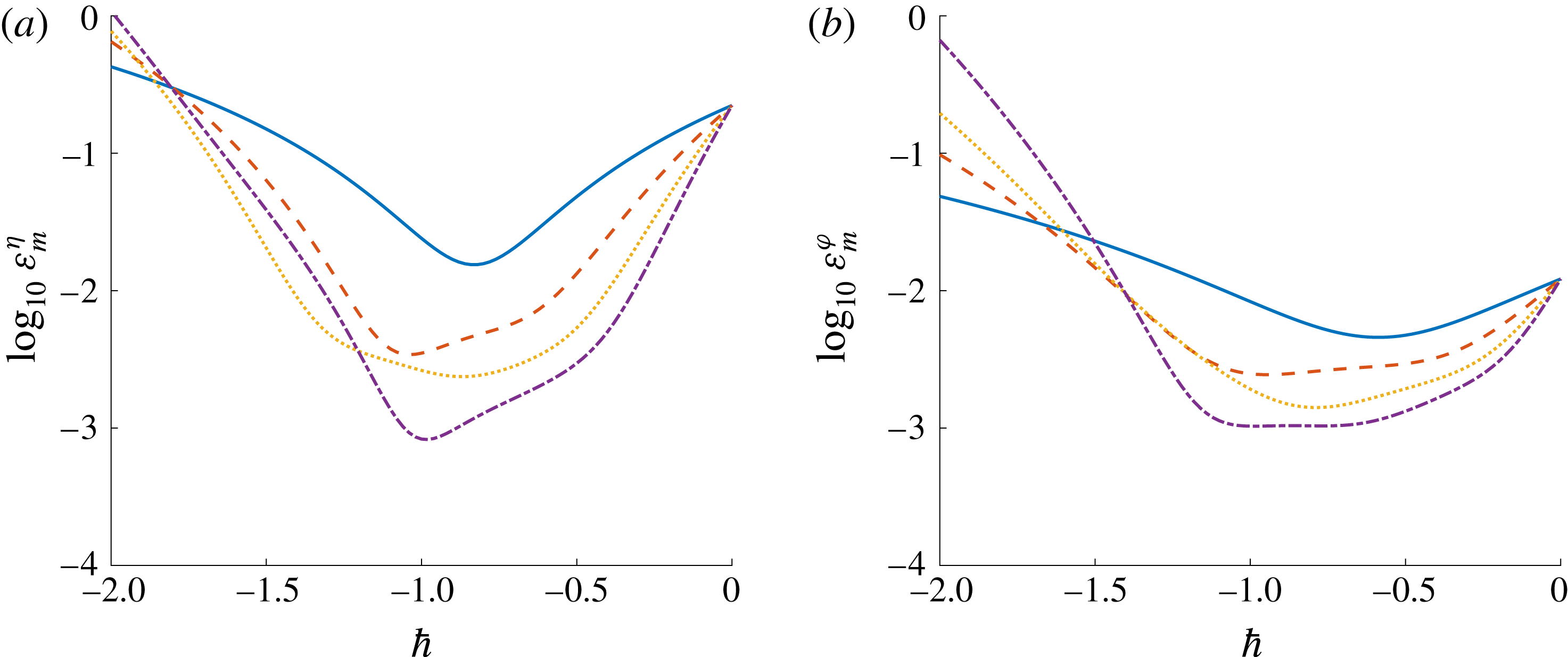
1 Introduction
Work on wave resonance was started by Phillips (Reference Phillips1960), who solved the nonlinear water wave equations by a perturbation method and found that a secular term may appear if the resonance criterion
 $$\begin{eqnarray}2\boldsymbol{k}_{1}-\boldsymbol{k}_{2}=\boldsymbol{k}_{0},\quad 2\unicode[STIX]{x1D714}_{1}-\unicode[STIX]{x1D714}_{2}=\unicode[STIX]{x1D714}_{0}\end{eqnarray}$$
is exactly satisfied, where
 $\boldsymbol{k}_{i}$
is the wavenumber and
 $\unicode[STIX]{x1D714}_{i}$
denotes the related linear angular frequency. In physics, the secular term indicates that the amplitude of a wave component would increase linearly with time, so a continuing flux of wave energy transfers from primary components to the resonant one. Later, Longuet-Higgins & Smith (Reference Longuet-Higgins and Smith1966) and McGoldrick et al. (Reference McGoldrick, Phillips, Huang and Hodgson1966) confirmed the resonance criterion (1.1) by experiments. In 1962, Benney (Reference Benney1962) proposed a model of exactly resonant waves with time-dependent periodically varying amplitudes, i.e. a periodically changing wave spectrum. Madsen & Fuhrman (Reference Madsen and Fuhrman2012) pointed out that, due to the singularities in the transfer functions, perturbation theory breaks down for steady-state resonant waves.
The real ocean surface is composed of a spectrum of wave frequencies, which participate in multiple resonances resulting in resonant waves which themselves satisfy resonance conditions (Alam, Liu & Yue Reference Alam, Liu and Yue2010). The dynamic spread of wave energy among multiple components is analytically intractable over time, so Alam et al. (Reference Alam, Liu and Yue2010) concluded that such a scenario is ideally suited to direct simulations such as the high-order spectrum method (Dommermuth & Yue Reference Dommermuth and Yue1987). The generalized Bragg scattering of surface waves by periodic bottom ripples was studied by Liu & Yue (Reference Liu and Yue1998), and later the amplitude evolution of multiple Bragg resonances of class III was considered by (Alam et al. Reference Alam, Liu and Yue2010).
Recently, based on the homotopy analysis method (HAM) (Liao Reference Liao1992, Reference Liao2003, Reference Liao2012; Zhong & Liao Reference Zhong and Liao2018), Liao (Reference Liao2011) reconsidered the nonlinear interactions between pairs of intersecting wave trains. When the resonance criterion (1.1) is exactly satisfied, Liao (Reference Liao2011) found that the secular term could be removed mathematically and steady-state waves with a time-independent spectrum were obtained. The existence of this kind of steady-state resonant waves was investigated experimentally in a basin at the State Key Laboratory of Ocean Engineering in Shanghai by Liu et al. (Reference Liu, Xu, Li, Peng, Alsaedi and Liao2015).
It should be noted that this is not the first time that a singularity problem has appeared in the study of nonlinear water waves. More than one and a half centuries ago, in the study of progressive periodic waves, Stokes (Reference Stokes1847) found that a perturbation-series approach would give rise to a spurious secular term, in contradiction to the periodic behaviour of the waves. Stokes (Reference Stokes1847) solved this problem by expanding the dispersion relationship into a perturbation series, a method now known as the Lindstedt–Poincaré method (Dingemans Reference Dingemans1997). The method of resolving the singularity is expected to bring a breakthrough in nonlinear water wave theory.
For a steady-state wave system, the Stokes wave (Stokes Reference Stokes1847) has the simplest spectrum as it contains only one non-trivial component. The next simplest spectrum corresponds to short-crested waves (Roberts Reference Roberts1983; Hammack, Henderson & Segur Reference Hammack, Henderson and Segur2005). It contains two non-trivial components propagating at an angle to each other with equal wavelengths and amplitudes. When three or more non-trivial components appear in the spectrum, resonance may appear, so the resonant interactions need to be considered and steady-state resonant waves are obtained (Liao Reference Liao2011; Liu et al. Reference Liu, Xu, Li, Peng, Alsaedi and Liao2015). For a discrete spectrum, more components are desirable for a representation of ocean waves. Compared with the Stokes wave and short-crested waves, steady-state resonant waves contain more non-trivial components; thus, they provide a more realistic description of real ocean waves and would serve as a general benchmark for the study of nonlinear wave evolution.
Liao (Reference Liao2011) resolved the singularity caused by single exact resonance and considered steady-state wave groups with three non-trivial components in deep water. Xu et al. (Reference Xu, Lin, Liao and Stiassnie2012) studied single exact resonance with three non-trivial components in finite water depths. Liu & Liao (Reference Liu and Liao2014) extended the work of Liao (Reference Liao2011) from a single quartet with three non-trivial components to coupled quartets with six non-trivial ones, and studied the coupled interactions among one exactly resonant set and six nearly resonant ones. To date, quite a few non-trivial components have been considered in the theoretical work on steady-state resonant waves. It should be noted that a system that admits one resonant set of waves often admits many resonant sets simultaneously (Hammack & Henderson Reference Hammack and Henderson1993). That is, waves often interact in coupled sets so that multiple resonances need to be considered. The simulations of nonlinear random water wave fields conducted by Annenkov & Shrira (Reference Annenkov and Shrira2006) demonstrated the key importance of near-resonant interactions: exact resonances can be excluded without a noticeable effect on the field evolution, provided that near-resonant interactions are retained. Besides, the exact resonance can be considered as a special case of the near resonance, i.e. the frequency mismatch in near resonance is zero. Therefore, more non-trivial components or, specifically, more nearly resonant components need to be considered in steady-state waves with general multiple resonances. It should be noted that more nearly resonant components imply that more small divisors, which are very challenging to resolve if classical perturbation methods are applied, would appear. Recently, Liao, Xu & Stiassnie (Reference Liao, Xu and Stiassnie2016) applied the HAM to resolve a small divisor caused by a single near resonance. However, the way in which to handle the small divisors caused by multiple near resonances is currently unknown. It is also unknown whether steady-state nearly resonant waves exist or not when more components join the resonance.
The study of steady-state resonant waves started with the weakly nonlinear cases in deep water considered by Liao (Reference Liao2011). Xu et al. (Reference Xu, Lin, Liao and Stiassnie2012), Liu & Liao (Reference Liu and Liao2014) and Liao et al. (Reference Liao, Xu and Stiassnie2016) extended the existing domain of steady-state resonant waves from different aspects, but still focused on weakly nonlinear wave groups. Finite amplitude wave groups have only been considered by Liu et al. (Reference Liu, Xu, Li, Peng, Alsaedi and Liao2015), where steady-state resonant waves were superimposed by several copropagating short-crested wave trains. No more finite amplitude steady-state exactly/nearly resonant wave groups have ever been reported. It should be noted that Liu & Liao (Reference Liu and Liao2014) found that small-amplitude steady-state resonant waves indeed form a continuum in the parameter space. Finite amplitude steady-state resonant wave groups need further investigation.
The objective of this paper is to investigate the finite amplitude steady-state wave groups with near resonances superimposed by multiple non-trivial components. The auxiliary linear operator and the initial guess in the framework of the HAM are further modified, so that small-divisor problems associated with the nearly resonant components are resolved, and theoretically no limit is set on the number of components considered in the resonant sets (§ 2.3). Weakly nonlinear wave systems are considered first (§ 3.1). As the nonlinearity increases, different initial guesses and auxiliary linear operators are considered in the HAM to search for possible steady-state waves (§ 3.2). The dependence of the number of solutions on the number of components comprising the resonance is analysed. Finally, the nonlinearity of wave groups is further increased so that finite amplitude wave groups are obtained (§ 3.3).
2 Mathematical formulae
2.1 Governing equation
We assume that the fluid is inviscid and incompressible, the flow is irrotational and the surface tension is neglected. Here,
 $(x,y,z)$
represents the usual Cartesian coordinate system, in which
 $(x,y)$
defines a horizontal plane located at the mean water level and
 $z$
is measured vertically upwards. The governing equations for deep-water waves read
 $$\begin{eqnarray}\displaystyle & \displaystyle \unicode[STIX]{x1D6FB}^{2}\unicode[STIX]{x1D711}=0,\quad -\infty <z<\unicode[STIX]{x1D702}(x,y,t), & \displaystyle\end{eqnarray}$$
 $$\begin{eqnarray}\displaystyle & \displaystyle {\displaystyle \frac{\unicode[STIX]{x2202}^{2}\unicode[STIX]{x1D711}}{\unicode[STIX]{x2202}t^{2}}}+g{\displaystyle \frac{\unicode[STIX]{x2202}\unicode[STIX]{x1D711}}{\unicode[STIX]{x2202}z}}+{\displaystyle \frac{\unicode[STIX]{x2202}|\unicode[STIX]{x1D735}\unicode[STIX]{x1D711}|^{2}}{\unicode[STIX]{x2202}t}}+\unicode[STIX]{x1D735}\unicode[STIX]{x1D711}\boldsymbol{\cdot }\unicode[STIX]{x1D735}\left({\displaystyle \frac{1}{2}}|\unicode[STIX]{x1D735}\unicode[STIX]{x1D711}|^{2}\right)=0,\quad \text{on }z=\unicode[STIX]{x1D702}(x,y,t), & \displaystyle\end{eqnarray}$$
 $$\begin{eqnarray}\displaystyle & \displaystyle g\unicode[STIX]{x1D702}+{\displaystyle \frac{\unicode[STIX]{x2202}\unicode[STIX]{x1D711}}{\unicode[STIX]{x2202}t}}+{\displaystyle \frac{1}{2}}|\unicode[STIX]{x1D735}\unicode[STIX]{x1D711}|^{2}=0,\quad \text{on }z=\unicode[STIX]{x1D702}(x,y,t), & \displaystyle\end{eqnarray}$$
 $$\begin{eqnarray}\displaystyle & \displaystyle {\displaystyle \frac{\unicode[STIX]{x2202}\unicode[STIX]{x1D711}}{\unicode[STIX]{x2202}z}}=0,\quad \text{as }z\rightarrow -\infty , & \displaystyle\end{eqnarray}$$
where
 $\unicode[STIX]{x1D711}$
denotes the velocity potential,
 $\unicode[STIX]{x1D702}$
is the free-surface elevation,
 $g$
is the gravity acceleration and
 $t$
is the time. We consider a wave system that consists of two primary progressive waves. Let
 $\boldsymbol{k}_{i}$
denote the wavenumber and
 $\unicode[STIX]{x1D70E}_{i}$
the actual angular frequency. For steady-state wave systems, all wave amplitudes
 $a_{i}$
, wavenumbers
 $\boldsymbol{k}_{i}$
and actual angular frequencies
 $\unicode[STIX]{x1D70E}_{i}$
are constant, i.e. independent of time. We write
 $$\begin{eqnarray}\unicode[STIX]{x1D709}_{i}=\boldsymbol{k}_{i}\boldsymbol{\cdot }\boldsymbol{r}-\unicode[STIX]{x1D70E}_{i}t,\quad i=1,2,\end{eqnarray}$$
where
 $\boldsymbol{r}=x\boldsymbol{i}+y\boldsymbol{j}$
. Therefore, in the new coordinate system
 $(\unicode[STIX]{x1D709}_{1},\unicode[STIX]{x1D709}_{2},z)$
, the original initial/boundary-value problem (2.1)–(2.4) can be transformed into a boundary-value problem governed by
 $$\begin{eqnarray}\mathop{\sum }_{i=1}^{2}\mathop{\sum }_{j=1}^{2}\boldsymbol{k}_{i}\boldsymbol{\cdot }\boldsymbol{k}_{j}{\displaystyle \frac{\unicode[STIX]{x2202}^{2}\unicode[STIX]{x1D711}}{\unicode[STIX]{x2202}\unicode[STIX]{x1D709}_{i}\unicode[STIX]{x2202}\unicode[STIX]{x1D709}_{j}}}+{\displaystyle \frac{\unicode[STIX]{x2202}^{2}\unicode[STIX]{x1D711}}{\unicode[STIX]{x2202}z^{2}}}=0,\quad -\infty <z<\unicode[STIX]{x1D702}(\unicode[STIX]{x1D709}_{1},\unicode[STIX]{x1D709}_{2})\end{eqnarray}$$
subject to the two boundary conditions on the unknown free surface
 $z=\unicode[STIX]{x1D702}(\unicode[STIX]{x1D709}_{1},\unicode[STIX]{x1D709}_{2})$
 $$\begin{eqnarray}\displaystyle {\mathcal{N}}_{1}[\unicode[STIX]{x1D711}] & = & \displaystyle \mathop{\sum }_{i=1}^{2}\mathop{\sum }_{j=1}^{2}\unicode[STIX]{x1D70E}_{i}\unicode[STIX]{x1D70E}_{j}{\displaystyle \frac{\unicode[STIX]{x2202}^{2}\unicode[STIX]{x1D711}}{\unicode[STIX]{x2202}\unicode[STIX]{x1D709}_{i}\unicode[STIX]{x2202}\unicode[STIX]{x1D709}_{j}}}+g{\displaystyle \frac{\unicode[STIX]{x2202}\unicode[STIX]{x1D711}}{\unicode[STIX]{x2202}z}}-2\mathop{\sum }_{i=1}^{2}\unicode[STIX]{x1D70E}_{i}{\displaystyle \frac{\unicode[STIX]{x2202}f}{\unicode[STIX]{x2202}\unicode[STIX]{x1D709}_{i}}}+\mathop{\sum }_{i=1}^{2}\mathop{\sum }_{j=1}^{2}\boldsymbol{k}_{i}\boldsymbol{\cdot }\boldsymbol{k}_{j}{\displaystyle \frac{\unicode[STIX]{x2202}\unicode[STIX]{x1D711}}{\unicode[STIX]{x2202}\unicode[STIX]{x1D709}_{i}}}{\displaystyle \frac{\unicode[STIX]{x2202}f}{\unicode[STIX]{x2202}\unicode[STIX]{x1D709}_{j}}}\nonumber\\ \displaystyle & & \displaystyle +\,{\displaystyle \frac{\unicode[STIX]{x2202}\unicode[STIX]{x1D711}}{\unicode[STIX]{x2202}z}}{\displaystyle \frac{\unicode[STIX]{x2202}f}{\unicode[STIX]{x2202}z}}=0,\end{eqnarray}$$
 $$\begin{eqnarray}{\mathcal{N}}_{2}[\unicode[STIX]{x1D702},\unicode[STIX]{x1D711}]=\unicode[STIX]{x1D702}-{\displaystyle \frac{1}{g}}\left(\mathop{\sum }_{i=1}^{2}\unicode[STIX]{x1D70E}_{i}{\displaystyle \frac{\unicode[STIX]{x2202}\unicode[STIX]{x1D711}}{\unicode[STIX]{x2202}\unicode[STIX]{x1D709}_{i}}}-f\right)=0\end{eqnarray}$$
and also the bottom condition
 $$\begin{eqnarray}{\displaystyle \frac{\unicode[STIX]{x2202}\unicode[STIX]{x1D711}}{\unicode[STIX]{x2202}z}}=0,\quad \text{as }z\rightarrow -\infty ,\end{eqnarray}$$
where
 ${\mathcal{N}}_{1}$
and
 ${\mathcal{N}}_{2}$
are the nonlinear differential operators and
 $$\begin{eqnarray}f={\displaystyle \frac{1}{2}}\left[\mathop{\sum }_{i=1}^{2}\mathop{\sum }_{j=1}^{2}\boldsymbol{k}_{i}\boldsymbol{\cdot }\boldsymbol{k}_{j}{\displaystyle \frac{\unicode[STIX]{x2202}\unicode[STIX]{x1D711}}{\unicode[STIX]{x2202}\unicode[STIX]{x1D709}_{i}}}{\displaystyle \frac{\unicode[STIX]{x2202}\unicode[STIX]{x1D711}}{\unicode[STIX]{x2202}\unicode[STIX]{x1D709}_{j}}}+\bigg({\displaystyle \frac{\unicode[STIX]{x2202}\unicode[STIX]{x1D711}}{\unicode[STIX]{x2202}z}}\bigg)^{2}\right].\end{eqnarray}$$
The wave elevation
 $\unicode[STIX]{x1D702}$
and velocity potential
 $\unicode[STIX]{x1D711}$
can be expressed in the form
 $$\begin{eqnarray}\displaystyle & \displaystyle \unicode[STIX]{x1D702}(\unicode[STIX]{x1D709}_{1},\unicode[STIX]{x1D709}_{2})=\mathop{\sum }_{m=-\infty }^{+\infty }\mathop{\sum }_{n=-\infty }^{+\infty }C_{m,n}^{\unicode[STIX]{x1D702}}\cos (m\unicode[STIX]{x1D709}_{1}+n\unicode[STIX]{x1D709}_{2}), & \displaystyle\end{eqnarray}$$
 $$\begin{eqnarray}\displaystyle & \displaystyle \unicode[STIX]{x1D711}(\unicode[STIX]{x1D709}_{1},\unicode[STIX]{x1D709}_{2},z)=\mathop{\sum }_{m=-\infty }^{+\infty }\mathop{\sum }_{n=-\infty }^{+\infty }C_{m,n}^{\unicode[STIX]{x1D711}}\unicode[STIX]{x1D6F9}_{m,n}(\unicode[STIX]{x1D709}_{1},\unicode[STIX]{x1D709}_{2},z), & \displaystyle\end{eqnarray}$$
with the definition
 $$\begin{eqnarray}\unicode[STIX]{x1D6F9}_{m,n}(\unicode[STIX]{x1D709}_{1},\unicode[STIX]{x1D709}_{2},z)=\sin (m\unicode[STIX]{x1D709}_{1}+n\unicode[STIX]{x1D709}_{2})\exp (|m\boldsymbol{k}_{1}+n\boldsymbol{k}_{2}|z),\end{eqnarray}$$
where
 $C_{m,n}^{\unicode[STIX]{x1D702}}$
and
 $C_{m,n}^{\unicode[STIX]{x1D711}}$
are constants to be determined. The constant
 $C_{m,n}^{\unicode[STIX]{x1D702}}$
denotes the amplitude of the wave component
 $\cos (m\unicode[STIX]{x1D709}_{1}+n\unicode[STIX]{x1D709}_{2})$
. It should be noted that
 $\unicode[STIX]{x1D711}(\unicode[STIX]{x1D709}_{1},\unicode[STIX]{x1D709}_{2},z)$
automatically satisfies the governing equation (2.6) and the bottom condition (2.9).
2.2 Solution procedure
The steady-state waves were obtained by means of the HAM for exact resonance (Liao Reference Liao2011) and near resonance (Liao et al.
Reference Liao, Xu and Stiassnie2016) in deep water, and extended by others for more complicated cases of exact resonance (Xu et al.
Reference Xu, Lin, Liao and Stiassnie2012; Liu & Liao Reference Liu and Liao2014). Detailed mathematical derivations can be found in these articles. For the sake of simplicity, we just give the most important formulae here. In the HAM-based approach, the solutions for the wave elevation
 $\unicode[STIX]{x1D702}$
and the velocity potential
 $\unicode[STIX]{x1D711}$
are approximated by the following two series:
 $$\begin{eqnarray}\displaystyle & \displaystyle \unicode[STIX]{x1D702}(\unicode[STIX]{x1D709}_{1},\unicode[STIX]{x1D709}_{2})=\mathop{\sum }_{m=1}^{+\infty }\unicode[STIX]{x1D702}_{m}(\unicode[STIX]{x1D709}_{1},\unicode[STIX]{x1D709}_{2}), & \displaystyle\end{eqnarray}$$
 $$\begin{eqnarray}\displaystyle & \displaystyle \unicode[STIX]{x1D711}(\unicode[STIX]{x1D709}_{1},\unicode[STIX]{x1D709}_{2},z)=\unicode[STIX]{x1D711}_{0}(\unicode[STIX]{x1D709}_{1},\unicode[STIX]{x1D709}_{2},z)+\mathop{\sum }_{m=1}^{+\infty }\unicode[STIX]{x1D711}_{m}(\unicode[STIX]{x1D709}_{1},\unicode[STIX]{x1D709}_{2},z), & \displaystyle\end{eqnarray}$$
which are governed by the high-order deformation equations
 $$\begin{eqnarray}\displaystyle & \displaystyle \unicode[STIX]{x1D702}_{m}(\unicode[STIX]{x1D709}_{1},\unicode[STIX]{x1D709}_{2})=c_{0}\unicode[STIX]{x1D6E5}_{m-1}^{\unicode[STIX]{x1D702}}(\unicode[STIX]{x1D709}_{1},\unicode[STIX]{x1D709}_{2})+\unicode[STIX]{x1D712}_{m}\unicode[STIX]{x1D702}_{m-1}(\unicode[STIX]{x1D709}_{1},\unicode[STIX]{x1D709}_{2}), & \displaystyle\end{eqnarray}$$
 $$\begin{eqnarray}\displaystyle & \displaystyle {\mathcal{L}}[\unicode[STIX]{x1D711}_{m}(\unicode[STIX]{x1D709}_{1},\unicode[STIX]{x1D709}_{2},z)]=c_{0}\unicode[STIX]{x1D6E5}_{m-1}^{\unicode[STIX]{x1D711}}(\unicode[STIX]{x1D709}_{1},\unicode[STIX]{x1D709}_{2})-\bar{S}_{m}(\unicode[STIX]{x1D709}_{1},\unicode[STIX]{x1D709}_{2})+\unicode[STIX]{x1D712}_{m}S_{m-1}(\unicode[STIX]{x1D709}_{1},\unicode[STIX]{x1D709}_{2}), & \displaystyle\end{eqnarray}$$
with the definition
 $\unicode[STIX]{x1D712}_{1}=0$
and
 $\unicode[STIX]{x1D712}_{m}=1$
for
 $m>1$
, where
 $\unicode[STIX]{x1D711}_{0}$
is an initial guess of the velocity potential
 $\unicode[STIX]{x1D711}$
,
 ${\mathcal{L}}$
is an auxiliary linear operator and
 $c_{0}$
is a convergence-control parameter. We choose the initial guess
 $\unicode[STIX]{x1D702}_{0}=0$
mainly because it is the simplest one and is also used by most traditional analytical methods. Up to the
 $m$
th order of approximation, all terms
 $\unicode[STIX]{x1D6E5}_{m-1}^{\unicode[STIX]{x1D702}}$
,
 $\unicode[STIX]{x1D6E5}_{m-1}^{\unicode[STIX]{x1D711}}$
,
 $\bar{S}_{m}$
and
 $S_{m-1}$
on the right-hand side of the high-order deformation equations (2.16) and (2.17) are already known and determined by
 $\unicode[STIX]{x1D702}_{j}$
and
 $\unicode[STIX]{x1D711}_{j}$
, with
 $j=0,1,2,\ldots ,m-1$
and
 $m\geqslant 1$
. The detailed expressions for
 $\unicode[STIX]{x1D6E5}_{m-1}^{\unicode[STIX]{x1D702}}$
and
 $\unicode[STIX]{x1D6E5}_{m-1}^{\unicode[STIX]{x1D711}}$
are shown in appendix A. It should be emphasized that, in the framework of the HAM, we have great freedom to choose the auxiliary linear operator
 ${\mathcal{L}}$
and the initial guess
 $\unicode[STIX]{x1D711}_{0}$
. The expressions for
 $\bar{S}_{m}$
and
 $S_{m-1}$
which depend on the choice of the auxiliary linear operator
 ${\mathcal{L}}$
are given in the next subsection.
2.3 Choice of auxiliary linear operator and initial potential
The key to the HAM approach is the choice of the auxiliary linear operator and the initial guess. The choices for single exact and near resonances are reviewed in § 2.3.1 and § 2.3.2 respectively. Then, the auxiliary linear operator and the initial guess for multiple near resonances are considered in § 2.3.3.
2.3.1 Single exact resonance
For a steady-state exact resonance,
 $$\begin{eqnarray}m_{\ast }\boldsymbol{k}_{1}+n_{\ast }\boldsymbol{k}_{2}=\boldsymbol{k}_{0},\quad m_{\ast }\unicode[STIX]{x1D714}_{1}+n_{\ast }\unicode[STIX]{x1D714}_{2}=\unicode[STIX]{x1D714}_{0},\end{eqnarray}$$
Liao (Reference Liao2011) chose the auxiliary linear operator
 $$\begin{eqnarray}{\mathcal{L}}_{a}[\unicode[STIX]{x1D711}]=\unicode[STIX]{x1D714}_{1}^{2}{\displaystyle \frac{\unicode[STIX]{x2202}^{2}\unicode[STIX]{x1D711}}{\unicode[STIX]{x2202}\unicode[STIX]{x1D709}_{1}^{2}}}+2\unicode[STIX]{x1D714}_{1}\unicode[STIX]{x1D714}_{2}{\displaystyle \frac{\unicode[STIX]{x2202}^{2}\unicode[STIX]{x1D711}}{\unicode[STIX]{x2202}\unicode[STIX]{x1D709}_{1}\unicode[STIX]{x2202}\unicode[STIX]{x1D709}_{2}}}+\unicode[STIX]{x1D714}_{2}^{2}{\displaystyle \frac{\unicode[STIX]{x2202}^{2}\unicode[STIX]{x1D711}}{\unicode[STIX]{x2202}\unicode[STIX]{x1D709}_{2}^{2}}}+g{\displaystyle \frac{\unicode[STIX]{x2202}\unicode[STIX]{x1D711}}{\unicode[STIX]{x2202}z}},\end{eqnarray}$$
with the property
 $$\begin{eqnarray}{\mathcal{L}}_{a}^{-1}[C\unicode[STIX]{x1D6F9}_{m,n}(\unicode[STIX]{x1D709}_{1},\unicode[STIX]{x1D709}_{2},z)]={\displaystyle \frac{C}{\unicode[STIX]{x1D706}_{m,n}^{a}}}\unicode[STIX]{x1D6F9}_{m,n}(\unicode[STIX]{x1D709}_{1},\unicode[STIX]{x1D709}_{2},z),\end{eqnarray}$$
where
 $\unicode[STIX]{x1D6F9}_{m,n}$
defined by (2.13) is the eigenfunction,
 $$\begin{eqnarray}\unicode[STIX]{x1D706}_{m,n}^{a}=g|m\boldsymbol{k}_{1}+n\boldsymbol{k}_{2}|-(m\unicode[STIX]{x1D714}_{1}+n\unicode[STIX]{x1D714}_{2})^{2}\end{eqnarray}$$
is the eigenvalue and
 $C$
is a constant related to the amplitude of the component
 $\cos (m\unicode[STIX]{x1D709}_{1}+n\unicode[STIX]{x1D709}_{2})$
. Based on the auxiliary linear operator (2.19),
 $\bar{S}_{m}$
and
 $S_{m}$
are defined as
 $$\begin{eqnarray}\displaystyle & \displaystyle \bar{S}_{m}(\unicode[STIX]{x1D709}_{1},\unicode[STIX]{x1D709}_{2})=\mathop{\sum }_{n=1}^{m-1}(\unicode[STIX]{x1D714}_{1}^{2}\unicode[STIX]{x1D6FD}_{2,0}^{m-n,n}+2\unicode[STIX]{x1D714}_{1}\unicode[STIX]{x1D714}_{2}\unicode[STIX]{x1D6FD}_{1,1}^{m-n,n}+\unicode[STIX]{x1D714}_{2}^{2}\unicode[STIX]{x1D6FD}_{0,2}^{m-n,n}+g\unicode[STIX]{x1D6FE}_{0,0}^{m-n,n}), & \displaystyle\end{eqnarray}$$
 $$\begin{eqnarray}\displaystyle & \displaystyle S_{m}(\unicode[STIX]{x1D709}_{1},\unicode[STIX]{x1D709}_{2})=\left(\unicode[STIX]{x1D714}_{1}^{2}\unicode[STIX]{x1D6FD}_{2,0}^{m,0}+2\unicode[STIX]{x1D714}_{1}\unicode[STIX]{x1D714}_{2}\unicode[STIX]{x1D6FD}_{1,1}^{m,0}+\unicode[STIX]{x1D714}_{2}^{2}\unicode[STIX]{x1D6FD}_{0,2}^{m,0}+g\unicode[STIX]{x1D6FE}_{0,0}^{m,0}\right)+\bar{S}_{m}. & \displaystyle\end{eqnarray}$$
Detailed expressions for
 $\unicode[STIX]{x1D6FD}_{2,0}^{m,n}$
,
 $\unicode[STIX]{x1D6FD}_{1,1}^{m,n}$
,
 $\unicode[STIX]{x1D6FD}_{0,2}^{m,n}$
and
 $\unicode[STIX]{x1D6FE}_{0,0}^{m,n}$
are given in (A 10) and (A 11).
Due to the linear dispersion relation, it holds that
 $\unicode[STIX]{x1D706}_{1,0}^{a}\equiv \unicode[STIX]{x1D706}_{0,1}^{a}\equiv 0$
. When the exact resonance criterion (2.18) is satisfied, we obtain
 $\unicode[STIX]{x1D706}_{m_{\ast },n_{\ast }}^{a}=0$
. Thus, the auxiliary linear operator (2.19) has three eigenvalues equal to zero. It should be noted that the traditional perturbation approach breaks down (Madsen & Fuhrman Reference Madsen and Fuhrman2012) as singularity appears when the inverse linear operator in (2.20) is applied on the resonant component
 $\unicode[STIX]{x1D6F9}_{m_{\ast },n_{\ast }}$
. In the HAM approach (Liao Reference Liao2011), two primary components
 $\unicode[STIX]{x1D6F9}_{1,0}$
,
 $\unicode[STIX]{x1D6F9}_{0,1}$
together with the exactly resonant one
 $\unicode[STIX]{x1D6F9}_{m_{\ast },n_{\ast }}$
are considered as homogeneous solutions to the auxiliary linear operator (2.19). The solution of the
 $m$
th-order approximation
 $\unicode[STIX]{x1D711}_{m}(\unicode[STIX]{x1D709}_{1},\unicode[STIX]{x1D709}_{2},z)$
reads
 $$\begin{eqnarray}\unicode[STIX]{x1D711}_{m}(\unicode[STIX]{x1D709}_{1},\unicode[STIX]{x1D709}_{2},z)=\unicode[STIX]{x1D711}_{m}^{\ast }(\unicode[STIX]{x1D709}_{1},\unicode[STIX]{x1D709}_{2},z)+A_{m,1}\unicode[STIX]{x1D6F9}_{1,0}+A_{m,2}\unicode[STIX]{x1D6F9}_{0,1}+A_{m,3}\unicode[STIX]{x1D6F9}_{m_{\ast },n_{\ast }},\end{eqnarray}$$
where
 $$\begin{eqnarray}\unicode[STIX]{x1D711}_{m}^{\ast }(\unicode[STIX]{x1D709}_{1},\unicode[STIX]{x1D709}_{2},z)={\mathcal{L}}_{a}^{-1}[c_{0}\unicode[STIX]{x1D6E5}_{m-1}^{\unicode[STIX]{x1D711}}(\unicode[STIX]{x1D709}_{1},\unicode[STIX]{x1D709}_{2})-\bar{S}_{m}(\unicode[STIX]{x1D709}_{1},\unicode[STIX]{x1D709}_{2})+\unicode[STIX]{x1D712}_{m}S_{m-1}(\unicode[STIX]{x1D709}_{1},\unicode[STIX]{x1D709}_{2})]\end{eqnarray}$$
is the particular solution of
 $\unicode[STIX]{x1D711}_{m}(\unicode[STIX]{x1D709}_{1},\unicode[STIX]{x1D709}_{2},z)$
, and the unknown constants
 $A_{m,1}$
,
 $A_{m,2}$
and
 $A_{m,3}$
are determined by avoiding the secular terms
 $\sin (\unicode[STIX]{x1D709}_{1})$
,
 $\sin (\unicode[STIX]{x1D709}_{2})$
and
 $\sin (m_{\ast }\unicode[STIX]{x1D709}_{1}+n_{\ast }\unicode[STIX]{x1D709}_{2})$
appearing on the right-hand side of the
 $(m+1)$
th-order deformation equation (2.17) for
 $\unicode[STIX]{x1D711}_{m+1}(\unicode[STIX]{x1D709}_{1},\unicode[STIX]{x1D709}_{2},z)$
(
 $m=1,2,\ldots$
). When
 $m=0$
, we get the initial guess of the velocity potential which contains three initial non-trivial components
 $$\begin{eqnarray}\unicode[STIX]{x1D711}_{0}(\unicode[STIX]{x1D709}_{1},\unicode[STIX]{x1D709}_{2},z)=A_{0,1}\unicode[STIX]{x1D6F9}_{1,0}+A_{0,2}\unicode[STIX]{x1D6F9}_{0,1}+A_{0,3}\unicode[STIX]{x1D6F9}_{m_{\ast },n_{\ast }}.\end{eqnarray}$$
2.3.2 Single near resonance
For near resonance, frequency detuning is introduced into the resonance criteria
 $$\begin{eqnarray}m_{\ast }\boldsymbol{k}_{1}+n_{\ast }\boldsymbol{k}_{2}=\boldsymbol{k}_{0},\quad m_{\ast }\unicode[STIX]{x1D714}_{1}+n_{\ast }\unicode[STIX]{x1D714}_{2}=\unicode[STIX]{x1D714}_{0}+\text{d}\unicode[STIX]{x1D714},\end{eqnarray}$$
with
 $\text{d}\unicode[STIX]{x1D714}$
denoting the angular frequency mismatch. It should be emphasized that unlike perturbation techniques, the HAM provides us with great freedom to choose the auxiliary linear operator. In order to seek the steady-state nearly resonant waves, Liao et al. (Reference Liao, Xu and Stiassnie2016) chose a generalized linear operator
 $$\begin{eqnarray}{\mathcal{L}}_{b}[\unicode[STIX]{x1D711}]=\unicode[STIX]{x1D714}_{1}^{2}{\displaystyle \frac{\unicode[STIX]{x2202}^{2}\unicode[STIX]{x1D711}}{\unicode[STIX]{x2202}\unicode[STIX]{x1D709}_{1}^{2}}}+\unicode[STIX]{x1D707}_{1}\unicode[STIX]{x1D714}_{1}\unicode[STIX]{x1D714}_{2}{\displaystyle \frac{\unicode[STIX]{x2202}^{2}\unicode[STIX]{x1D711}}{\unicode[STIX]{x2202}\unicode[STIX]{x1D709}_{1}\unicode[STIX]{x2202}\unicode[STIX]{x1D709}_{2}}}+\unicode[STIX]{x1D714}_{2}^{2}{\displaystyle \frac{\unicode[STIX]{x2202}^{2}\unicode[STIX]{x1D711}}{\unicode[STIX]{x2202}\unicode[STIX]{x1D709}_{2}^{2}}}+g{\displaystyle \frac{\unicode[STIX]{x2202}\unicode[STIX]{x1D711}}{\unicode[STIX]{x2202}z}}\end{eqnarray}$$
with the property
 $$\begin{eqnarray}{\mathcal{L}}_{b}^{-1}[\unicode[STIX]{x1D6F9}_{m,n}(\unicode[STIX]{x1D709}_{1},\unicode[STIX]{x1D709}_{2},z)]={\displaystyle \frac{\unicode[STIX]{x1D6F9}_{m,n}(\unicode[STIX]{x1D709}_{1},\unicode[STIX]{x1D709}_{2},z)}{\unicode[STIX]{x1D706}_{m,n}^{b}}},\end{eqnarray}$$
where
 $$\begin{eqnarray}\unicode[STIX]{x1D707}_{1}={\displaystyle \frac{g|m_{\ast }\boldsymbol{k}_{1}+n_{\ast }\boldsymbol{k}_{2}|-(m_{\ast }^{2}\unicode[STIX]{x1D714}_{1}^{2}+n_{\ast }^{2}\unicode[STIX]{x1D714}_{2}^{2})}{m_{\ast }n_{\ast }\unicode[STIX]{x1D714}_{1}\unicode[STIX]{x1D714}_{2}}}\end{eqnarray}$$
is a constant and
 $$\begin{eqnarray}\unicode[STIX]{x1D706}_{m,n}^{b}=g|m\boldsymbol{k}_{1}+n\boldsymbol{k}_{2}|-(m^{2}\unicode[STIX]{x1D714}_{1}^{2}+\unicode[STIX]{x1D707}_{1}mn\unicode[STIX]{x1D714}_{1}\unicode[STIX]{x1D714}_{2}+n^{2}\unicode[STIX]{x1D714}_{2}^{2})\end{eqnarray}$$
is the corresponding eigenvalue. Based on the generalized linear operator (2.28),
 $\bar{S}_{m}$
and
 $S_{m}$
are defined as
 $$\begin{eqnarray}\displaystyle & \displaystyle \bar{S}_{m}(\unicode[STIX]{x1D709}_{1},\unicode[STIX]{x1D709}_{2})=\mathop{\sum }_{n=1}^{m-1}(\unicode[STIX]{x1D714}_{1}^{2}\unicode[STIX]{x1D6FD}_{2,0}^{m-n,n}+\unicode[STIX]{x1D707}_{1}\unicode[STIX]{x1D714}_{1}\unicode[STIX]{x1D714}_{2}\unicode[STIX]{x1D6FD}_{1,1}^{m-n,n}+\unicode[STIX]{x1D714}_{2}^{2}\unicode[STIX]{x1D6FD}_{0,2}^{m-n,n}+g\unicode[STIX]{x1D6FE}_{0,0}^{m-n,n}), & \displaystyle\end{eqnarray}$$
 $$\begin{eqnarray}\displaystyle & \displaystyle S_{m}(\unicode[STIX]{x1D709}_{1},\unicode[STIX]{x1D709}_{2})=(\unicode[STIX]{x1D714}_{1}^{2}\unicode[STIX]{x1D6FD}_{2,0}^{m,0}+\unicode[STIX]{x1D707}_{1}\unicode[STIX]{x1D714}_{1}\unicode[STIX]{x1D714}_{2}\unicode[STIX]{x1D6FD}_{1,1}^{m,0}+\unicode[STIX]{x1D714}_{2}^{2}\unicode[STIX]{x1D6FD}_{0,2}^{m,0}+g\unicode[STIX]{x1D6FE}_{0,0}^{m,0})+\bar{S}_{m}. & \displaystyle\end{eqnarray}$$
It should be noted that, if the original linear operator (2.19) is used for the near resonance (2.27), we will get a small eigenfunction
 $\unicode[STIX]{x1D706}_{m_{\ast },n_{\ast }}^{a}=-(2\sqrt{g|m_{\ast }\boldsymbol{ k}_{1}+n_{\ast }\boldsymbol{ k}_{2}|}+\text{d}\unicode[STIX]{x1D714})\,\text{d}\unicode[STIX]{x1D714}$
in the denominator of (2.20). This small divisor is hard to deal with especially for a nearly resonant component with a small angular frequency mismatch
 $\text{d}\unicode[STIX]{x1D714}$
. The constant
 $\unicode[STIX]{x1D707}_{1}$
in (2.28) is defined to enforce
 $\unicode[STIX]{x1D706}_{m_{\ast },n_{\ast }}^{b}=0$
, so the nearly resonant component
 $\unicode[STIX]{x1D6F9}_{m_{\ast ,\unicode[STIX]{x1D704}},n_{\ast ,\unicode[STIX]{x1D704}}}$
can be considered as a homogeneous solution to the generalized linear operator (2.28). Three zero eigenvalues
 $\unicode[STIX]{x1D706}_{1,0}^{b}=\unicode[STIX]{x1D706}_{0,1}^{b}=\unicode[STIX]{x1D706}_{m_{\ast },n_{\ast }}^{b}=0$
can be obtained and the near resonance (2.27) can then be handled in exactly the same way as the exact resonance (2.18) by means of the generalized linear operator (2.28). It should be noted that the mismatch
 $\text{d}\unicode[STIX]{x1D714}$
does not occur in (2.30) and (2.31) so that we can transform the small divisor associated with the nearly resonant component
 $1/\unicode[STIX]{x1D706}_{m_{\ast },n_{\ast }}^{a}$
to the singularity associated with the exactly resonant one
 $1/\unicode[STIX]{x1D706}_{m_{\ast },n_{\ast }}^{b}$
. The generalized linear operator (2.28) works for the exact resonance (2.18) as well, since an exact resonance can be considered as a special near resonance when
 $\text{d}\unicode[STIX]{x1D714}=0$
in (2.27). The solution of the
 $m$
th-order approximation
 $\unicode[STIX]{x1D711}_{m}(\unicode[STIX]{x1D709}_{1},\unicode[STIX]{x1D709}_{2},z)$
reads
 $$\begin{eqnarray}\unicode[STIX]{x1D711}_{m}(\unicode[STIX]{x1D709}_{1},\unicode[STIX]{x1D709}_{2},z)=\unicode[STIX]{x1D711}_{m}^{\ast }(\unicode[STIX]{x1D709}_{1},\unicode[STIX]{x1D709}_{2},z)+A_{m,1}\unicode[STIX]{x1D6F9}_{1,0}+A_{m,2}\unicode[STIX]{x1D6F9}_{0,1}+A_{m,3}\unicode[STIX]{x1D6F9}_{m_{\ast },n_{\ast }},\end{eqnarray}$$
where
 $\unicode[STIX]{x1D711}_{m}^{\ast }(\unicode[STIX]{x1D709}_{1},\unicode[STIX]{x1D709}_{2},z)$
is the particular solution of
 $\unicode[STIX]{x1D711}_{m}(\unicode[STIX]{x1D709}_{1},\unicode[STIX]{x1D709}_{2},z)$
defined as
 $$\begin{eqnarray}\unicode[STIX]{x1D711}_{m}^{\ast }(\unicode[STIX]{x1D709}_{1},\unicode[STIX]{x1D709}_{2},z)={\mathcal{L}}_{b}^{-1}[c_{0}\unicode[STIX]{x1D6E5}_{m-1}^{\unicode[STIX]{x1D711}}(\unicode[STIX]{x1D709}_{1},\unicode[STIX]{x1D709}_{2})-\bar{S}_{m}(\unicode[STIX]{x1D709}_{1},\unicode[STIX]{x1D709}_{2})+\unicode[STIX]{x1D712}_{m}S_{m-1}(\unicode[STIX]{x1D709}_{1},\unicode[STIX]{x1D709}_{2})],\end{eqnarray}$$
and the unknown constants
 $A_{m,1}$
,
 $A_{m,2}$
and
 $A_{m,3}$
are determined so that the coefficients of the terms
 $\sin (\unicode[STIX]{x1D709}_{1})$
,
 $\sin (\unicode[STIX]{x1D709}_{2})$
and
 $\sin (m_{\ast }\unicode[STIX]{x1D709}_{1}+n_{\ast }\unicode[STIX]{x1D709}_{2})$
on the right-hand side of the
 $(m+1)$
th-order deformation equation (2.17) for
 $\unicode[STIX]{x1D711}_{m+1}(\unicode[STIX]{x1D709}_{1},\unicode[STIX]{x1D709}_{2},z)$
(
 $m=1,2,\ldots$
) are equal to zero. When
 $m=0$
, we get the initial guess of the velocity potential which contains three initial non-trivial components,
 $$\begin{eqnarray}\unicode[STIX]{x1D711}_{0}(\unicode[STIX]{x1D709}_{1},\unicode[STIX]{x1D709}_{2},z)=A_{0,1}\unicode[STIX]{x1D6F9}_{1,0}+A_{0,2}\unicode[STIX]{x1D6F9}_{0,1}+A_{0,3}\unicode[STIX]{x1D6F9}_{m_{\ast },n_{\ast }}.\end{eqnarray}$$
2.3.3 Multiple near resonances
Let us consider a wave system with
 $l$
nearly resonant components (
 $\boldsymbol{k}_{0,1}$
,
 $\boldsymbol{k}_{0,2},\ldots ,\boldsymbol{k}_{0,l}$
) that are generated by two primary components (
 $\boldsymbol{k}_{1}$
and
 $\boldsymbol{k}_{2}$
). It satisfies the near resonance criteria
 $$\begin{eqnarray}m_{\ast ,\unicode[STIX]{x1D704}}\boldsymbol{k}_{1}+n_{\ast ,\unicode[STIX]{x1D704}}\boldsymbol{k}_{2}=\boldsymbol{k}_{0,\unicode[STIX]{x1D704}},\quad m_{\ast ,\unicode[STIX]{x1D704}}\unicode[STIX]{x1D714}_{1}+n_{\ast ,\unicode[STIX]{x1D704}}\unicode[STIX]{x1D714}_{2}=\unicode[STIX]{x1D714}_{0,\unicode[STIX]{x1D704}}+\text{d}\unicode[STIX]{x1D714}_{\unicode[STIX]{x1D704}},\quad \unicode[STIX]{x1D704}=1,2,\ldots ,l,\end{eqnarray}$$
where
 $\text{d}\unicode[STIX]{x1D714}_{\unicode[STIX]{x1D704}}$
is a small real number that represents the angular frequency mismatch of the
 $\unicode[STIX]{x1D704}$
th resonant component. The two primary components together with the
 $l$
nearly resonant ones are defined as the initial non-trivial components.
For multiple near resonances (2.37), the generalized linear operator (2.28) for a single near resonance breaks down as the small divisor appears for every nearly resonant component. Fortunately, the freedom in the choice of the auxiliary linear operator and the initial guess in the framework of the HAM provides an opportunity to completely resolve the small divisors caused by the abovementioned multiple near resonances. In this paper, we consider the following auxiliary linear operator:
 $$\begin{eqnarray}{\mathcal{L}}_{c}[\unicode[STIX]{x1D711}]=\unicode[STIX]{x1D714}_{1}^{2}{\displaystyle \frac{\unicode[STIX]{x2202}^{2}\unicode[STIX]{x1D711}}{\unicode[STIX]{x2202}\unicode[STIX]{x1D709}_{1}^{2}}}+\unicode[STIX]{x1D707}_{2}(m,n)\unicode[STIX]{x1D714}_{1}\unicode[STIX]{x1D714}_{2}{\displaystyle \frac{\unicode[STIX]{x2202}^{2}\unicode[STIX]{x1D711}}{\unicode[STIX]{x2202}\unicode[STIX]{x1D709}_{1}\unicode[STIX]{x2202}\unicode[STIX]{x1D709}_{2}}}+\unicode[STIX]{x1D714}_{2}^{2}{\displaystyle \frac{\unicode[STIX]{x2202}^{2}\unicode[STIX]{x1D711}}{\unicode[STIX]{x2202}\unicode[STIX]{x1D709}_{2}^{2}}}+g{\displaystyle \frac{\unicode[STIX]{x2202}\unicode[STIX]{x1D711}}{\unicode[STIX]{x2202}z}},\end{eqnarray}$$
with the property
 $$\begin{eqnarray}{\mathcal{L}}_{c}^{-1}[\unicode[STIX]{x1D6F9}_{m,n}(\unicode[STIX]{x1D709}_{1},\unicode[STIX]{x1D709}_{2},z)]={\displaystyle \frac{\unicode[STIX]{x1D6F9}_{m,n}(\unicode[STIX]{x1D709}_{1},\unicode[STIX]{x1D709}_{2},z)}{\unicode[STIX]{x1D706}_{m,n}^{c}}},\end{eqnarray}$$
where
 $$\begin{eqnarray}\unicode[STIX]{x1D707}_{2}(m,n)=\left\{\begin{array}{@{}ll@{}}{\displaystyle \frac{g|m\boldsymbol{k}_{1}+n\boldsymbol{k}_{2}|-(m^{2}\unicode[STIX]{x1D714}_{1}^{2}+n^{2}\unicode[STIX]{x1D714}_{2}^{2})}{mn\unicode[STIX]{x1D714}_{1}\unicode[STIX]{x1D714}_{2}}},\quad & m=m_{\ast ,\unicode[STIX]{x1D704}},n=n_{\ast ,\unicode[STIX]{x1D704}},\\ 2, & \text{else}\end{array}\right.\end{eqnarray}$$
is a piecewise function depending on
 $m$
and
 $n$
in
 $\unicode[STIX]{x1D711}(\unicode[STIX]{x1D709}_{1},\unicode[STIX]{x1D709}_{2},z)$
(2.12) and
 $$\begin{eqnarray}\unicode[STIX]{x1D706}_{m,n}^{c}=g|m\boldsymbol{k}_{1}+n\boldsymbol{k}_{2}|-(m^{2}\unicode[STIX]{x1D714}_{1}^{2}+\unicode[STIX]{x1D707}_{2}(m,n)mn\unicode[STIX]{x1D714}_{1}\unicode[STIX]{x1D714}_{2}+n^{2}\unicode[STIX]{x1D714}_{2}^{2})\end{eqnarray}$$
is the corresponding eigenvalue. Based on the generalized linear operator (2.38),
 $\bar{S}_{m}$
and
 $S_{m}$
are defined as
 $$\begin{eqnarray}\displaystyle & \displaystyle \bar{S}_{m}(\unicode[STIX]{x1D709}_{1},\unicode[STIX]{x1D709}_{2})=\mathop{\sum }_{n=1}^{m-1}(\unicode[STIX]{x1D714}_{1}^{2}\unicode[STIX]{x1D6FD}_{2,0}^{m-n,n}+\unicode[STIX]{x1D707}_{2}(m,n)\unicode[STIX]{x1D714}_{1}\unicode[STIX]{x1D714}_{2}\unicode[STIX]{x1D6FD}_{1,1}^{m-n,n}+\unicode[STIX]{x1D714}_{2}^{2}\unicode[STIX]{x1D6FD}_{0,2}^{m-n,n}+g\unicode[STIX]{x1D6FE}_{0,0}^{m-n,n}), & \displaystyle\end{eqnarray}$$
 $$\begin{eqnarray}\displaystyle & \displaystyle S_{m}(\unicode[STIX]{x1D709}_{1},\unicode[STIX]{x1D709}_{2})=(\unicode[STIX]{x1D714}_{1}^{2}\unicode[STIX]{x1D6FD}_{2,0}^{m,0}+\unicode[STIX]{x1D707}_{2}(m,n)\unicode[STIX]{x1D714}_{1}\unicode[STIX]{x1D714}_{2}\unicode[STIX]{x1D6FD}_{1,1}^{m,0}+\unicode[STIX]{x1D714}_{2}^{2}\unicode[STIX]{x1D6FD}_{0,2}^{m,0}+g\unicode[STIX]{x1D6FE}_{0,0}^{m,0})+\bar{S}_{m}. & \displaystyle\end{eqnarray}$$
If the auxiliary linear operator (2.19) is still applied for multiple near resonances (2.37), we will get small eigenvalues
 $\unicode[STIX]{x1D706}_{m_{\ast ,\unicode[STIX]{x1D704}},n_{\ast ,\unicode[STIX]{x1D704}}}^{a}$
proportional to the angular frequency mismatch
 $\text{d}\unicode[STIX]{x1D714}_{\unicode[STIX]{x1D704}}$
in the denominator of (2.20). A large-amplitude related constant
 $C$
together with a small eigenvalue
 $\unicode[STIX]{x1D706}_{m_{\ast ,\unicode[STIX]{x1D704}},n_{\ast ,\unicode[STIX]{x1D704}}}^{a}$
turns out to be a large coefficient
 $C/\unicode[STIX]{x1D706}_{m_{\ast ,\unicode[STIX]{x1D704}},n_{\ast ,\unicode[STIX]{x1D704}}}^{a}$
without physical meaning for the nearly resonant component
 $\unicode[STIX]{x1D6F9}_{m_{\ast ,\unicode[STIX]{x1D704}},n_{\ast ,\unicode[STIX]{x1D704}}}(\unicode[STIX]{x1D709}_{1},\unicode[STIX]{x1D709}_{2},z)$
in (2.20). The piecewise function
 $\unicode[STIX]{x1D707}_{2}(m,n)$
in (2.40) is determined to enforce the related eigenvalue
 $\unicode[STIX]{x1D706}_{m_{\ast ,\unicode[STIX]{x1D704}},n_{\ast ,\unicode[STIX]{x1D704}}}^{c}=0$
, so the initial non-trivial nearly resonant components
 $\unicode[STIX]{x1D6F9}_{m_{\ast ,\unicode[STIX]{x1D704}},n_{\ast ,\unicode[STIX]{x1D704}}}$
can be considered as homogeneous solutions to the auxiliary linear operator (2.38) since
 $\unicode[STIX]{x1D706}_{1,0}=\unicode[STIX]{x1D706}_{0,1}=\unicode[STIX]{x1D706}_{m_{\ast ,\unicode[STIX]{x1D704}},n_{\ast ,\unicode[STIX]{x1D704}}}^{c}=0$
. Every near resonance in (2.37) can then be handled exactly in the same way as the exact resonance (2.18) by the auxiliary linear operator (2.38). That is, the piecewise function
 $\unicode[STIX]{x1D707}_{2}(m,n)$
in the auxiliary linear operator (2.38) transforms the small divisors associated with non-trivial nearly resonant components
 $1/\unicode[STIX]{x1D706}_{m_{\ast },n_{\ast }}^{a}$
to the singularities associated with exactly resonant ones
 $1/\unicode[STIX]{x1D706}_{m_{\ast },n_{\ast }}^{c}$
. It should be noted that the new auxiliary linear operator (2.38) is a further generalization of the generalized auxiliary linear operator (2.28) proposed by Liao (Reference Liao2011). Besides, multiple exact resonances can be considered as a special case of the multiple near resonances with
 $\text{d}\unicode[STIX]{x1D714}_{i}=0$
in (2.37).
The solution of the
 $m$
th-order approximation
 $\unicode[STIX]{x1D711}_{m}(\unicode[STIX]{x1D709}_{1},\unicode[STIX]{x1D709}_{2},z)$
reads
 $$\begin{eqnarray}\unicode[STIX]{x1D711}_{m}(\unicode[STIX]{x1D709}_{1},\unicode[STIX]{x1D709}_{2},z)=\unicode[STIX]{x1D711}_{m}^{\ast }(\unicode[STIX]{x1D709}_{1},\unicode[STIX]{x1D709}_{2},z)+A_{m,1}\unicode[STIX]{x1D6F9}_{1,0}+A_{m,2}\unicode[STIX]{x1D6F9}_{0,1}+\mathop{\sum }_{\unicode[STIX]{x1D704}=1}^{l}A_{m,2+\unicode[STIX]{x1D704}}\unicode[STIX]{x1D6F9}_{m_{\ast ,\unicode[STIX]{x1D704}},n_{\ast ,\unicode[STIX]{x1D704}}},\end{eqnarray}$$
where
 $$\begin{eqnarray}\unicode[STIX]{x1D711}_{m}^{\ast }(\unicode[STIX]{x1D709}_{1},\unicode[STIX]{x1D709}_{2},z)={\mathcal{L}}_{c}^{-1}[c_{0}\unicode[STIX]{x1D6E5}_{m-1}^{\unicode[STIX]{x1D711}}(\unicode[STIX]{x1D709}_{1},\unicode[STIX]{x1D709}_{2})-\bar{S}_{m}(\unicode[STIX]{x1D709}_{1},\unicode[STIX]{x1D709}_{2})+\unicode[STIX]{x1D712}_{m}S_{m-1}(\unicode[STIX]{x1D709}_{1},\unicode[STIX]{x1D709}_{2})]\end{eqnarray}$$
is the particular solution of
 $\unicode[STIX]{x1D711}_{m}(\unicode[STIX]{x1D709}_{1},\unicode[STIX]{x1D709}_{2},z)$
, and the unknown constant
 $A_{m,i}$
is determined by removing the secular terms
 $\sin (\unicode[STIX]{x1D709}_{1})$
,
 $\sin (\unicode[STIX]{x1D709}_{2})$
and
 $\sin (m_{\ast ,\unicode[STIX]{x1D704}}\unicode[STIX]{x1D709}_{1}+n_{\ast ,\unicode[STIX]{x1D704}}\unicode[STIX]{x1D709}_{2})$
on the right-hand side of the
 $(m+1)$
th-order deformation equation (2.17) for
 $\unicode[STIX]{x1D711}_{m+1}(\unicode[STIX]{x1D709}_{1},\unicode[STIX]{x1D709}_{2},z)$
(
 $m=1,2,\ldots$
).
The initial guess of the velocity potential reads
 $$\begin{eqnarray}\unicode[STIX]{x1D711}_{0}(\unicode[STIX]{x1D709}_{1},\unicode[STIX]{x1D709}_{2},z)=A_{0,1}\unicode[STIX]{x1D6F9}_{1,0}+A_{0,2}\unicode[STIX]{x1D6F9}_{0,1}+\mathop{\sum }_{\unicode[STIX]{x1D704}=1}^{l}A_{0,2+\unicode[STIX]{x1D704}}\unicode[STIX]{x1D6F9}_{m_{\ast ,\unicode[STIX]{x1D704}},n_{\ast ,\unicode[STIX]{x1D704}}},\end{eqnarray}$$
where the coefficient
 $A_{0,i}$
is determined by avoiding the secular terms or small divisors in the first-order approximation
 $\unicode[STIX]{x1D711}_{1}(\unicode[STIX]{x1D709}_{1},\unicode[STIX]{x1D709}_{2},z)$
. For non-resonant waves, the initial guess (2.46) just contains the two primary waves, i.e.
 $l=0$
. For small-amplitude exact or near resonance waves, one non-trivial resonant component is considered in the initial guess (2.46) (
 $l=1$
). As the nonlinearity increases, an additional wave component would join the exact or near resonance due to the nonlinear interactions. The wave energy distribution among the more resonant components suggests that more non-trivial resonant components need to be considered in the initial guess (2.46), which will be shown later in this paper.
For simplicity, resonant waves with only two primary components have been considered in this paper. The choice of the auxiliary linear operator, the initial guess and the related solution procedures can easily be extended for more general cases with multiple primary components.
3 Results and analysis
Let
 $\unicode[STIX]{x1D6FC}$
denote the angle between primary components
 $\boldsymbol{k}_{1}$
and
 $\boldsymbol{k}_{2}$
, let
 $\unicode[STIX]{x1D70F}=k_{2}/k_{1}$
be the wavenumber ratio and let
 $\unicode[STIX]{x1D716}=\unicode[STIX]{x1D70E}_{1}/\unicode[STIX]{x1D714}_{1}=\unicode[STIX]{x1D70E}_{2}/\unicode[STIX]{x1D714}_{2}$
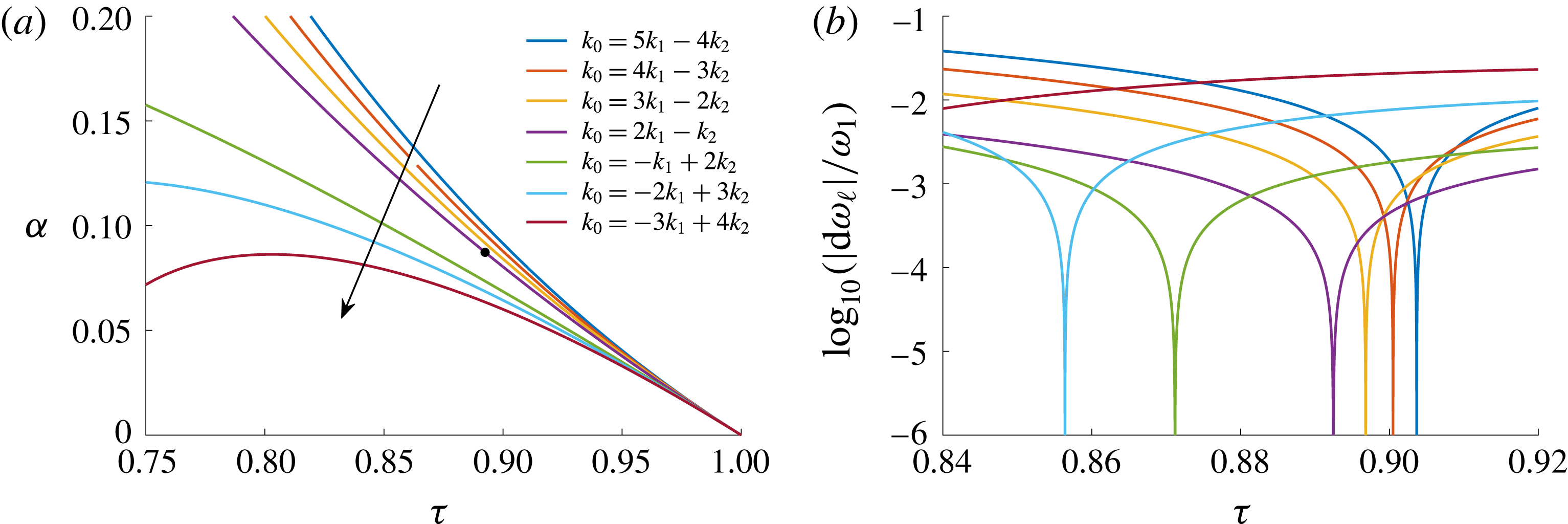
be the dimensionless frequency to quantify the nonlinearity of the wave system. Figure 1(a) shows the linear resonance curves of seven adjacent resonant sets (2.18) in the wavevector space
 $(\unicode[STIX]{x1D70F},\unicode[STIX]{x1D6FC})$
. The filled circle corresponds to the exact resonance considered by Liao (Reference Liao2011). The resonance curves around the filled circle stay quite close to each other, which indicates that different wave components may interact with one another so that multiple resonances may occur. For a given angle
 $\unicode[STIX]{x1D6FC}=\unicode[STIX]{x03C0}/36$
, figure 1(b) shows the frequency detuning of the same seven adjacent resonant components. As the wavenumber ratio
 $\unicode[STIX]{x1D70F}$
increases, the component with the smallest frequency detuning changes from one to the next. For each resonant component, the interval of
 $\unicode[STIX]{x1D70F}$
with angular frequency mismatch
 $\log _{10}(|\text{d}\unicode[STIX]{x1D714}_{i}|/\unicode[STIX]{x1D714}_{1})<-2$
overlaps with the intervals of nearby ones. Nearby components need to be considered for possible multiple near resonances.
(a) The linear resonance curves of (2.18) for seven adjacent resonant sets in the wavevector space
 $(\unicode[STIX]{x1D70F},\unicode[STIX]{x1D6FC})$
. The filled circle corresponds to the exact resonance considered by Liao (Reference Liao2011). (b) The angular frequency detuning of seven adjacent resonant components with increased wavenumber ratio
 $\unicode[STIX]{x1D70F}$
when the angle
 $\unicode[STIX]{x1D6FC}=\unicode[STIX]{x03C0}/36$
.

3.1 Weakly nonlinear wave groups
For weakly nonlinear wave systems, Liao et al. (Reference Liao, Xu and Stiassnie2016) considered the single nearly resonant set
 $$\begin{eqnarray}2\boldsymbol{k}_{1}-\boldsymbol{k}_{2}=\boldsymbol{k}_{0},\quad 2\unicode[STIX]{x1D714}_{1}-\unicode[STIX]{x1D714}_{2}=\unicode[STIX]{x1D714}_{0}+\text{d}\unicode[STIX]{x1D714}\end{eqnarray}$$
in the case of
 $$\begin{eqnarray}\unicode[STIX]{x1D6FC}=\unicode[STIX]{x03C0}/36,\quad 0.89\leqslant \unicode[STIX]{x1D70F}\leqslant 0.895,\quad \unicode[STIX]{x1D716}=1.0003,\end{eqnarray}$$
with the generalized linear operator (2.28). Multiple solutions were obtained and the energy distribution was verified by Zakharov’s equation.
To investigate further whether nearby resonant components interact with one another at the end of the solution domain considered by Liao et al. (Reference Liao, Xu and Stiassnie2016), we consider two nearly resonant components in the auxiliary linear operator (2.38) and initial potential (2.46). We take the two groups of solutions found by Liao et al. (Reference Liao, Xu and Stiassnie2016) at
 $\unicode[STIX]{x1D70F}=0.89$
as an example; the calculations are carried out beyond the domain
 $0.89\leqslant \unicode[STIX]{x1D70F}\leqslant 0.895$
until one or more components have lost their energy and leave the resonance with one or two components. Specifically, we consider the components
 $\unicode[STIX]{x1D6F9}_{2,-1}$
and
 $\unicode[STIX]{x1D6F9}_{1,-2}$
in the initial potential (2.46) for
 $\unicode[STIX]{x1D70F}<0.89$
in group 1, and the components
 $\unicode[STIX]{x1D6F9}_{2,-1}$
and
 $\unicode[STIX]{x1D6F9}_{3,-2}$
in the initial potential (2.46) for
 $\unicode[STIX]{x1D70F}>0.895$
in group 2. The piecewise function
 $\unicode[STIX]{x1D707}_{2}(m,n)$
in the auxiliary linear operator (2.38) changes accordingly with the two nearly resonant components.
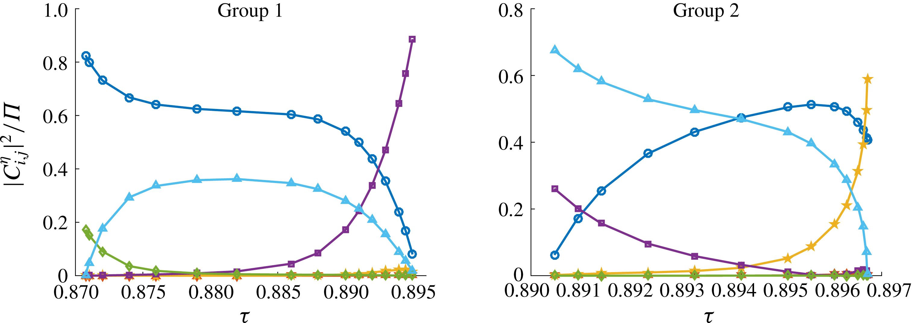
The wave energy distribution of the six largest components
 $|C_{i,j}^{\unicode[STIX]{x1D702}}|^{2}/\unicode[STIX]{x1D6F1}$
of the resonant system (2.37) in the case of dimensionless frequency
 $\unicode[STIX]{x1D716}=1.0003$
and angle
 $\unicode[STIX]{x1D6FC}=\unicode[STIX]{x03C0}/36$
with various wavenumber ratios
 $\unicode[STIX]{x1D70F}$
: line with circles,
 $|C_{1,0}^{\unicode[STIX]{x1D702}}|^{2}/\unicode[STIX]{x1D6F1}$
; line with triangles,
 $|C_{0,1}^{\unicode[STIX]{x1D702}}|^{2}/\unicode[STIX]{x1D6F1}$
; line with squares,
 $|C_{2,-1}^{\unicode[STIX]{x1D702}}|^{2}/\unicode[STIX]{x1D6F1}$
; line with pentagrams,
 $|C_{3,-2}^{\unicode[STIX]{x1D702}}|^{2}/\unicode[STIX]{x1D6F1}$
; line with hexagrams,
 $|C_{4,-3}^{\unicode[STIX]{x1D702}}|^{2}/\unicode[STIX]{x1D6F1}$
; line with diamonds,
 $|C_{-1,2}^{\unicode[STIX]{x1D702}}|^{2}/\unicode[STIX]{x1D6F1}$
.

Figure 2 shows the wave energy distribution of the six largest components (two primary components together with four nearly resonant ones)
 $|C_{i,j}^{\unicode[STIX]{x1D702}}|^{2}/\unicode[STIX]{x1D6F1}$
for the resonant system (2.37) in the case of dimensionless frequency
 $\unicode[STIX]{x1D716}=1.0003$
and angle
 $\unicode[STIX]{x1D6FC}=\unicode[STIX]{x03C0}/36$
with various wavenumber ratios
 $\unicode[STIX]{x1D70F}$
. The total wave energy
 $\unicode[STIX]{x1D6F1}=\sum _{m=0}^{+\infty }\sum _{n=-\infty }^{+\infty }(C_{m,n}^{\unicode[STIX]{x1D702}})^{2}$
is mainly contained by three components belonging to one resonant set. Energy transfer due to resonant interaction among different components is obvious, but no coupled resonances can be identified. In group 1, the energy contained by the component
 $\cos (\unicode[STIX]{x1D709}_{1}-2\unicode[STIX]{x1D709}_{2})$
(
 $|C_{1,-2}^{\unicode[STIX]{x1D702}}|^{2}/\unicode[STIX]{x1D6F1}$
) decreases from
 $17.2\,\%$
at
 $\unicode[STIX]{x1D70F}=0.87075$
to
 $0\,\%$
at
 $\unicode[STIX]{x1D70F}=0.895$
; meanwhile, the energy contained by the component
 $\cos (2\unicode[STIX]{x1D709}_{1}-\unicode[STIX]{x1D709}_{2})$
(
 $|C_{2,-1}^{\unicode[STIX]{x1D702}}|^{2}/\unicode[STIX]{x1D6F1}$
) increases from
 $0\,\%$
to
 $88.6\,\%$
. In group 2, the energy contained by the component
 $\cos (2\unicode[STIX]{x1D709}_{1}-\unicode[STIX]{x1D709}_{2})$
(
 $|C_{2,-1}^{\unicode[STIX]{x1D702}}|^{2}/\unicode[STIX]{x1D6F1}$
) decreases from
 $26.1\,\%$
at
 $\unicode[STIX]{x1D70F}=0.89$
to
 $0.6\,\%$
at
 $\unicode[STIX]{x1D70F}=0.89669$
; meanwhile, the energy contained by the component
 $\cos (3\unicode[STIX]{x1D709}_{1}-2\unicode[STIX]{x1D709}_{2})$
(
 $|C_{3,-2}^{\unicode[STIX]{x1D702}}|^{2}/\unicode[STIX]{x1D6F1}$
) increases from
 $0.2\,\%$
to
 $56.2\,\%$
. This transfer of energy between nearby nearly resonant components for weakly nonlinear wave groups indicates that coupled resonances among multiple nearly resonant components may occur for finite amplitude wave groups.
More calculations were carried out in the wavevector space
 $(\unicode[STIX]{x1D70F},\unicode[STIX]{x1D6FC})$
for weakly nonlinear cases (
 $\unicode[STIX]{x1D716}=1.0003$
). The related energy distribution analyses confirm the continuum of steady-state resonances in the wavevector space
 $(\unicode[STIX]{x1D70F},\unicode[STIX]{x1D6FC})$
and the phenomenon of energy transfer among nearby nearly resonant components.
3.2 Wave groups with increased components
More nearly resonant components are considered in wave groups with increased nonlinearity to further check the existence of steady-state multiple near resonances. Without loss of generality, we consider the near resonance case
 $$\begin{eqnarray}\unicode[STIX]{x1D6FC}=\unicode[STIX]{x03C0}/36,\quad \unicode[STIX]{x1D70F}=0.89,\end{eqnarray}$$
with dimensionless frequency
 $\unicode[STIX]{x1D716}$
increased from 1.0003 to 1.005. Different combinations of the four largest nearly resonant components at
 $\unicode[STIX]{x1D716}=1.0003$
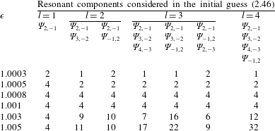
are considered as non-trivial components in the initial guess (2.46) to search for possible steady-state solutions. As shown in table 1, the number of nearly resonant components
 $l$
increases step by step from one to four. The term
 $\unicode[STIX]{x1D707}_{2}(m,n)$
in the auxiliary linear operator (2.38) changes accordingly. When three or fewer resonant components are considered as initial non-trivial ones, the coupled nonlinear algebraic equations for the coefficients
 $A_{0,i}$
are solved globally in the calculation of the first-order approximation. For four initial non-trivial nearly resonant components, the resulting algebraic equations are too complicated and time consuming to solve globally. Instead, a root searching procedure based on the partial solver ‘FindRoot’ in Mathematica is applied. Table 1 shows that the number of real solutions for the coefficients
 $A_{0,i}$
increases with the dimensionless frequency
 $\unicode[STIX]{x1D716}$
, especially when three or four nearly resonant components (
 $l=3,4$
) are considered. For example, for four nearly resonant components, the number of algebraic solutions increases from 1 at dimensionless frequency
 $\unicode[STIX]{x1D716}=1.0003$
to 32 at
 $\unicode[STIX]{x1D716}=1.005$
. The increased number of algebraic solutions for larger values of the dimensionless frequency
 $\unicode[STIX]{x1D716}$
indicates that more steady-state nearly resonant waves may exist when the nonlinearity increases, if more non-trivial resonant components are considered in the solution procedure.
The number of real solutions for the initial guess coefficients
 $A_{0,i}$
in (2.46), for angle
 $\unicode[STIX]{x1D6FC}=\unicode[STIX]{x03C0}/36$
and wavenumber ratio
 $\unicode[STIX]{x1D70F}=0.89$
.

The number of convergent solutions for resonant wave systems (2.37), for angle
 $\unicode[STIX]{x1D6FC}=\unicode[STIX]{x03C0}/36$
and wavenumber ratio
 $\unicode[STIX]{x1D70F}=0.89$
.
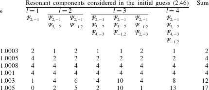
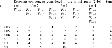
Table 2 shows the number of convergent solutions based on the initial guesses listed in table 1. When three or fewer initial non-trivial resonant components are considered, the number of convergent solutions first increases and then decreases with respect to the dimensionless frequency
 $\unicode[STIX]{x1D716}$
. When four initial non-trivial resonant components are considered, the number of convergent solutions increases with
 $\unicode[STIX]{x1D716}$
up to
 $1.005$
. It should be noted that at
 $\unicode[STIX]{x1D716}=1.005$
, no convergent solution is obtained for
 $l=1$
(corresponding to only one resonant component) and the number of solutions increases for
 $l=2,3,4$
(corresponding to two, three and four resonant ones). Steady-state waves with multiple near resonances indeed exist, and more nearly resonant components need to be considered as initial non-trivial ones in the solution procedure when the nonlinearity increases. The last column in table 2 shows that the total number of convergent solutions increases from
 $2$
at
 $\unicode[STIX]{x1D716}=1.0003$
to
 $17$
at
 $\unicode[STIX]{x1D716}=1.005$
, i.e. the number of steady-state wave groups increases with respect to the nonlinearity of wave groups when more components join the near resonance. This indicates that the probability of existence of steady-state resonant waves increases with the nonlinearity of wave groups.
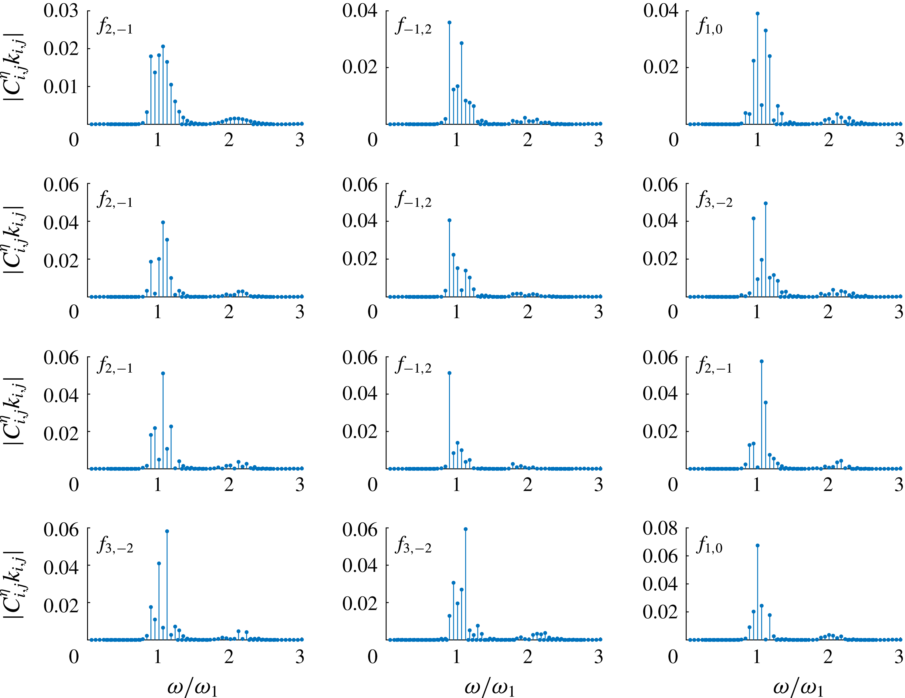
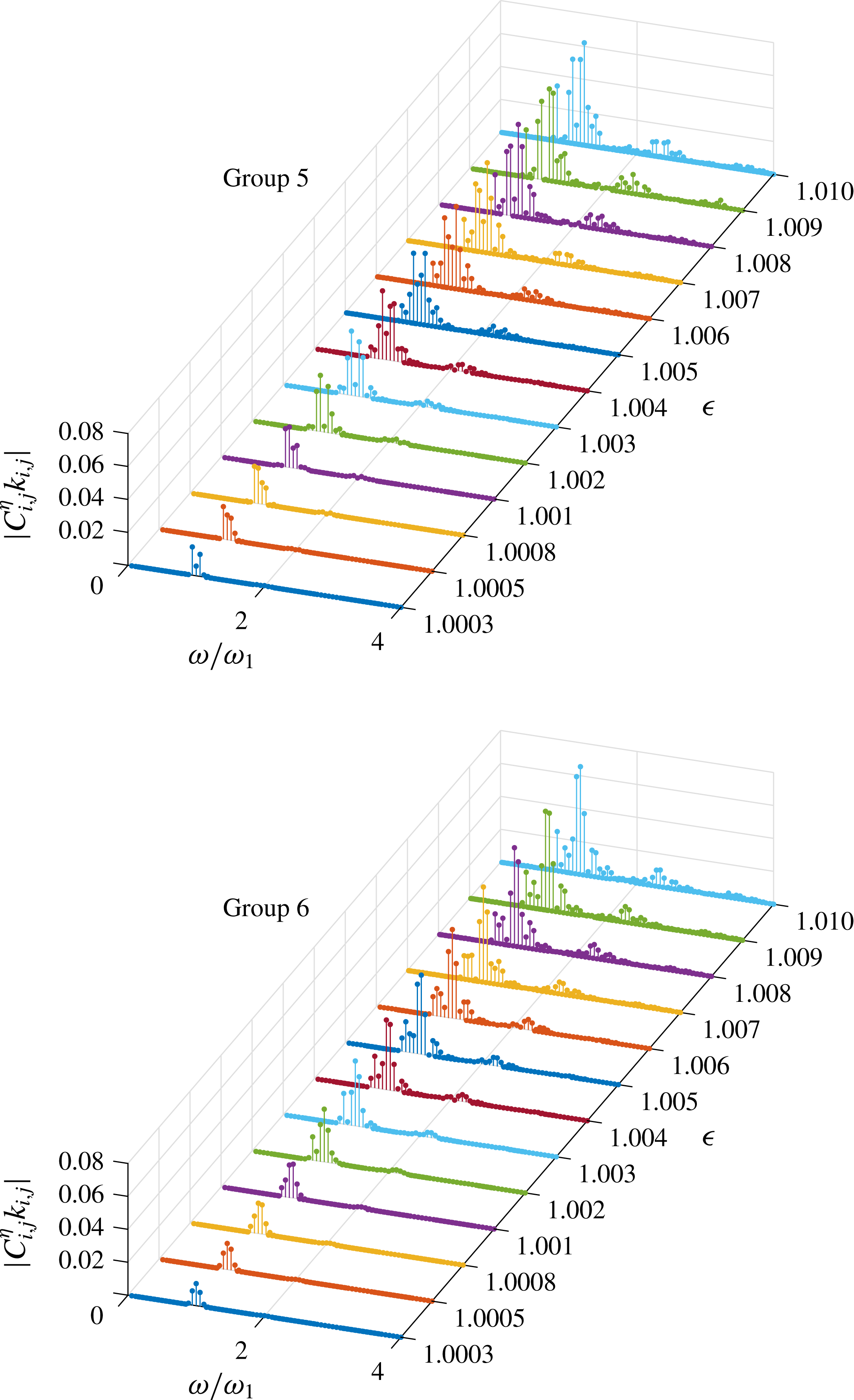
Figures 3 and 4 show the amplitude spectra of steady-state waves for dimensionless frequencies of
 $\unicode[STIX]{x1D716}=1.003$
and
 $1.005$
respectively. The wave spectra are ordered based on the maximum dimensionless amplitude
 $|C_{i,j}^{\unicode[STIX]{x1D702}}k_{i,j}|$
, from smallest to largest. Moreover, within each spectrum, the dominant frequency
 $f_{i,j}$
that is surrounded by other smaller peaks is indicated (
 $f_{i,j}$
denotes the frequency of the component
 $\cos (i\unicode[STIX]{x1D709}_{1}+j\unicode[STIX]{x1D709}_{2})$
). The spectral shape, especially the dominant frequency
 $f_{i,j}$
together with the related amplitude
 $|C_{i,j}^{\unicode[STIX]{x1D702}}k_{i,j}|$
, changes among different groups. The evidence of multiple resonances in steady-state waves is clearly shown. Compared with the spectra at
 $\unicode[STIX]{x1D716}=1.003$
, two additional dominant frequencies
 $f_{0,1}$
and
 $f_{4,-3}$
appear in the spectra at
 $\unicode[STIX]{x1D716}=1.005$
. This suggests that more components indeed join the resonance. Besides, the maximum amplitudes
 $|C_{i,j}^{\unicode[STIX]{x1D702}}k_{i,j}|$
increase and five more time-independent spectra are obtained at
 $\unicode[STIX]{x1D716}=1.005$
. Spectral analysis confirms that both the number of components comprising the resonance and the number of steady-state waves increase with the nonlinearity of the wave groups.
The amplitude spectrum
 $|C_{i,j}^{\unicode[STIX]{x1D702}}k_{i,j}|$
of wave groups in the case of dimensionless frequency
 $\unicode[STIX]{x1D716}=1.003$
, angle
 $\unicode[STIX]{x1D6FC}=\unicode[STIX]{x03C0}/36$
and wavenumber ratio
 $\unicode[STIX]{x1D70F}=0.89$
. Here,
 $f_{i,j}$
denotes the dominant frequency.

The same as figure 3, except that
 $\unicode[STIX]{x1D716}=1.005$
.

3.3 Finite amplitude wave groups
The dimensionless frequency
 $\unicode[STIX]{x1D716}$
is further increased to search for finite amplitude steady-state nearly resonant wave groups.
When the wavevectors of the primary components are given, the eigenvalue
 $\unicode[STIX]{x1D706}_{m_{\ast ,\unicode[STIX]{x1D704}},n_{\ast ,\unicode[STIX]{x1D704}}}^{a}$
of every nearly resonant component is known and is determined by the resonance criterion (2.37), while the amplitude related constant
 $C$
is unknown and can only be determined during the calculations. It is hard to predetermine which nearly resonant component should be considered as the initial non-trivial one in the solution procedure that determines the initial guess (2.46) and the auxiliary linear operator (2.38). To guide the choice of the initial guess and the auxiliary linear operator, the magnitude of the angular frequency mismatch
 $\text{d}\unicode[STIX]{x1D714}_{\unicode[STIX]{x1D704}}$
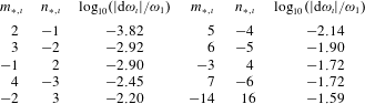
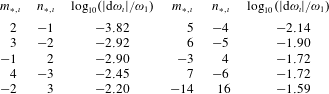
is analysed. Table 3 shows the 10 nearly resonant components with the smallest angular frequency mismatch
 $\log _{10}(|\text{d}\unicode[STIX]{x1D714}_{\unicode[STIX]{x1D704}}|/\unicode[STIX]{x1D714}_{1})$
in the case of angle
 $\unicode[STIX]{x1D6FC}=\unicode[STIX]{x03C0}/36$
and wavenumber ratio
 $\unicode[STIX]{x1D70F}=0.89$
. Results based on combinations of the first four components in § 3.2 show that the number of initial non-trivial components increases with the dimensionless frequency when
 $\unicode[STIX]{x1D716}\in [1.0003,1.005]$
. As the dimensionless frequency
 $\unicode[STIX]{x1D716}$
further increases, more nearly resonant components are suggested to be considered as the initial non-trivial ones. The remaining six components in table 3 could be provided as the possible non-trivial ones in the initial guess (2.46).
The 10 near-resonant components with the smallest angular frequency mismatch
 $\log _{10}(|\text{d}\unicode[STIX]{x1D714}_{\unicode[STIX]{x1D704}}|/\unicode[STIX]{x1D714}_{1})$
in the case of angle
 $\unicode[STIX]{x1D6FC}=\unicode[STIX]{x03C0}/36$
and wavenumber ratio
 $\unicode[STIX]{x1D70F}=0.89$
.
Taking the first two groups of solutions (at
 $\unicode[STIX]{x1D716}=1.0003$
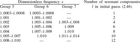
) in table 2 as an example (groups 5 and 6), the number of resonant components
 $l$
considered for different dimensionless frequencies
 $\unicode[STIX]{x1D716}$
is shown in table 4. Within each group, the number of resonant components
 $l$
increases, so that three significant digits can be obtained for the unknown constants
 $C_{m,n}^{\unicode[STIX]{x1D702}}$
and
 $C_{m,n}^{\unicode[STIX]{x1D711}}$
in (2.11) and (2.12). It should be noted that in group 5, the number of resonant components
 $l$
increases up to 12 when
 $\unicode[STIX]{x1D716}\geqslant 1.008$
. For each dimensionless frequency
 $\unicode[STIX]{x1D716}$
, the corresponding coupled nonlinear algebraic equations for
 $A_{0,i}$
in the initial guess (2.46) are solved by the partial root solver described in § 3.2, with the solution of
 $A_{0,i}$
at a slightly smaller value of
 $\unicode[STIX]{x1D716}$
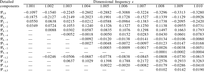
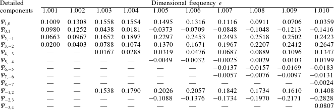
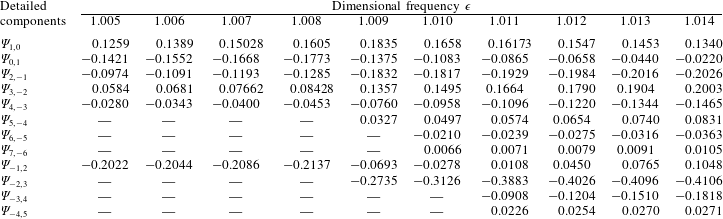
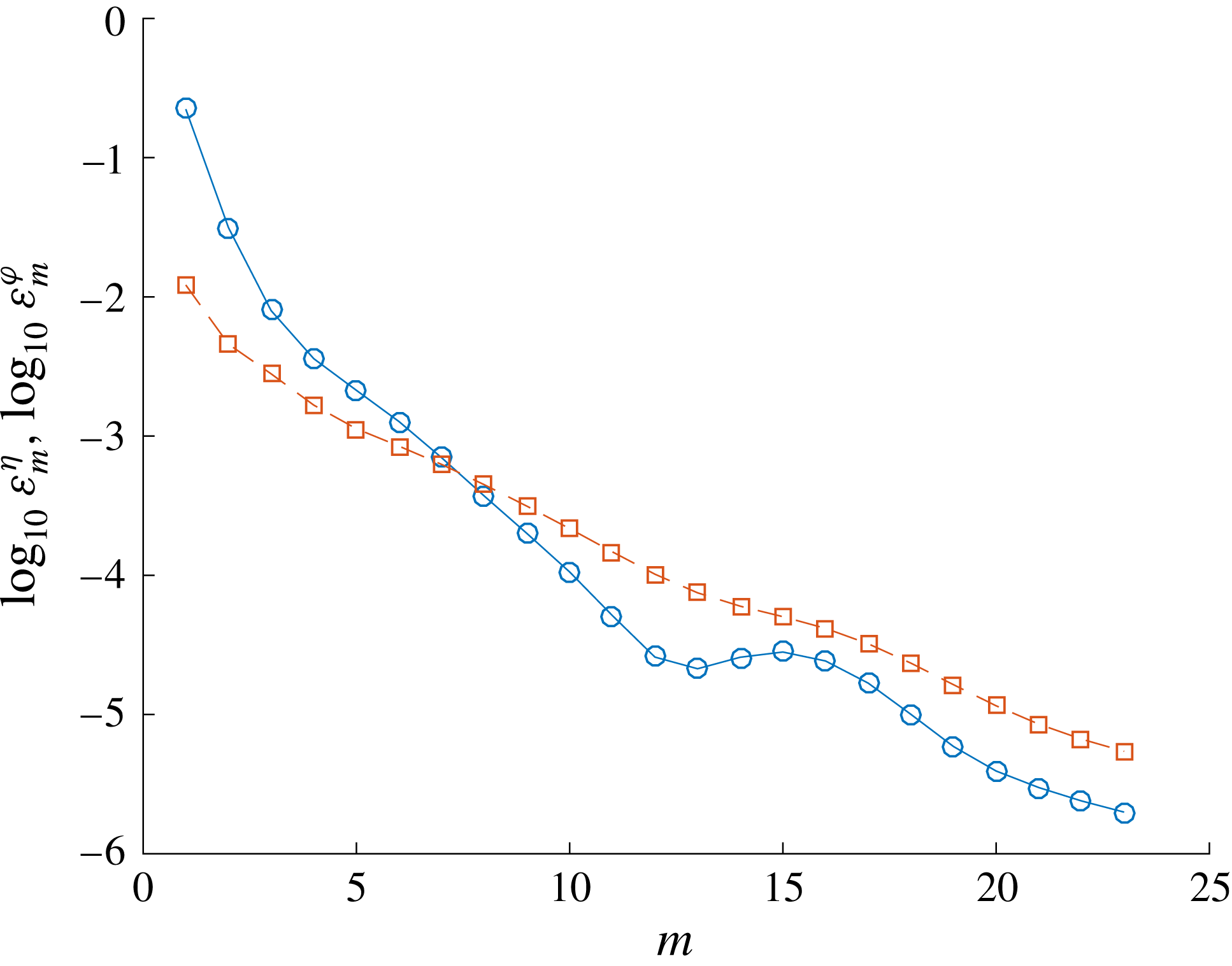
serving as the initial solution. Detailed components together with related coefficients in the initial potential (2.46) for groups 5 and 6 are shown in tables 5 and 6 in appendix B. The convergence of the related high-order approximations obtained by the HAM for multiple nearly resonant wave groups is shown in appendix C.
The number of resonant components in the initial guess (2.46) with increased dimensionless frequency
 $\unicode[STIX]{x1D716}$
for groups 5, 6 and 7 in the case of angle
 $\unicode[STIX]{x1D6FC}=\unicode[STIX]{x03C0}/36$
and wavenumber ratio
 $\unicode[STIX]{x1D70F}=0.89$
.

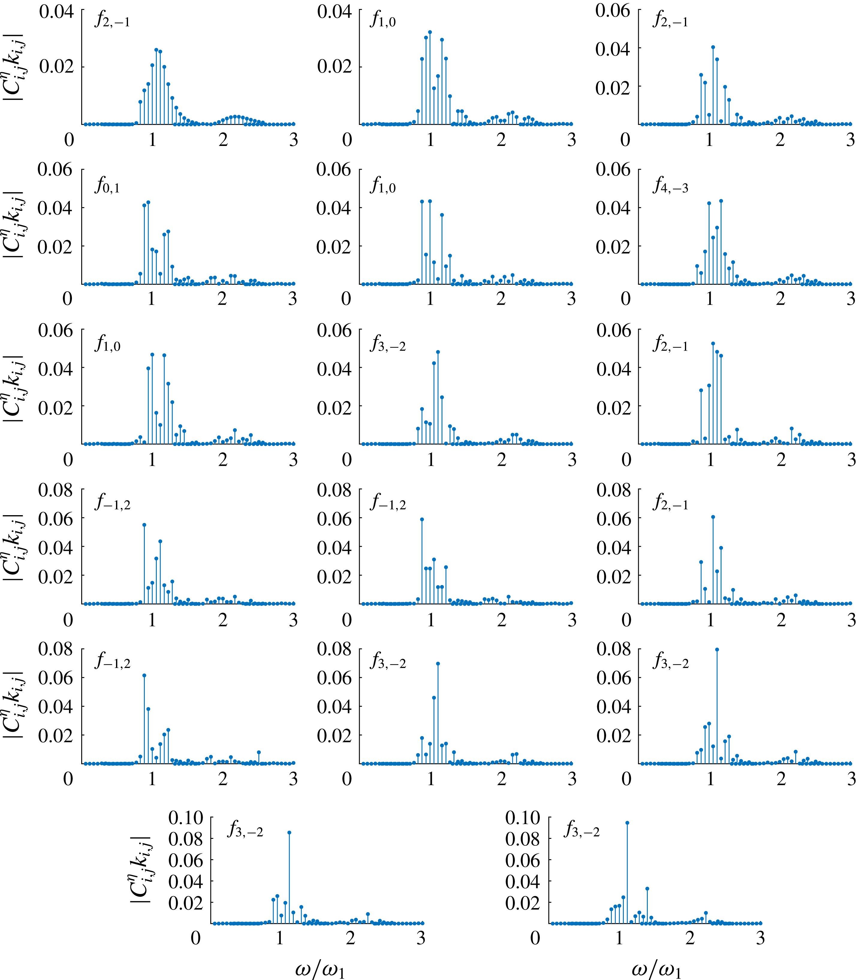
Figure 5 shows the amplitude spectra of groups 5 and 6 when the dimensionless frequency
 $\unicode[STIX]{x1D716}$
increases from
 $1.0003$
to
 $1.010$
. More components indeed join the near resonances and the frequency bands broaden with respect to the increased dimensionless frequency
 $\unicode[STIX]{x1D716}$
. The wave group energy is mainly contained by components near the first-order primary ones, with some by second-order bound ones. No spectral symmetry is found for all values of
 $\unicode[STIX]{x1D716}$
considered. The dimensionless amplitudes of components with
 $|C_{i,j}^{\unicode[STIX]{x1D702}}k_{i,j}|>0.01$
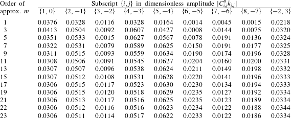
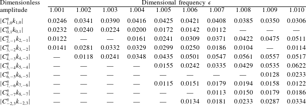
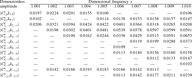
in groups 5 and 6 are shown in tables 9 and 10 in appendix D.
The amplitude spectra
 $|C_{i,j}^{\unicode[STIX]{x1D702}}k_{i,j}|$
in the case of angle
 $\unicode[STIX]{x1D6FC}=\unicode[STIX]{x03C0}/36$
and wavenumber ratio
 $\unicode[STIX]{x1D70F}=0.89$
with increased dimensionless frequency
 $\unicode[STIX]{x1D716}$
.

Within each group, the amplitude of each component may either increase or decrease with the dimensionless frequency
 $\unicode[STIX]{x1D716}$
, whereas the amplitude of the whole wave group increases continuously. We define the wave steepness as
 $$\begin{eqnarray}H_{steepness}=k_{d}{\displaystyle \frac{\max [\unicode[STIX]{x1D702}(\unicode[STIX]{x1D709}_{1},\unicode[STIX]{x1D709}_{2})]-\min [\unicode[STIX]{x1D702}(\unicode[STIX]{x1D709}_{1},\unicode[STIX]{x1D709}_{2})]}{2}},\quad \unicode[STIX]{x1D709}_{i}\in [0,2\unicode[STIX]{x03C0}],\end{eqnarray}$$
where
 $k_{d}$
is the wavenumber corresponding to the dominant frequency. It is found that, at
 $\unicode[STIX]{x1D716}=1.010$
, the wave steepness
 $H_{steepness}$
reaches
 $0.22$
and
 $0.21$
in groups 5 and 6 respectively. For wave groups with discrete spectra, the large-amplitude case with
 $H_{steepness}=0.21$
was investigated by Shemer et al. (Reference Shemer, Jiao, Kit and Agnon2001) for the evolution of the nonlinear wave field along a tank. Therefore, it is reasonable to conclude that finite amplitude steady-state nearly resonant wave groups are obtained in groups 5 and 6 at
 $\unicode[STIX]{x1D716}=1.010$
.
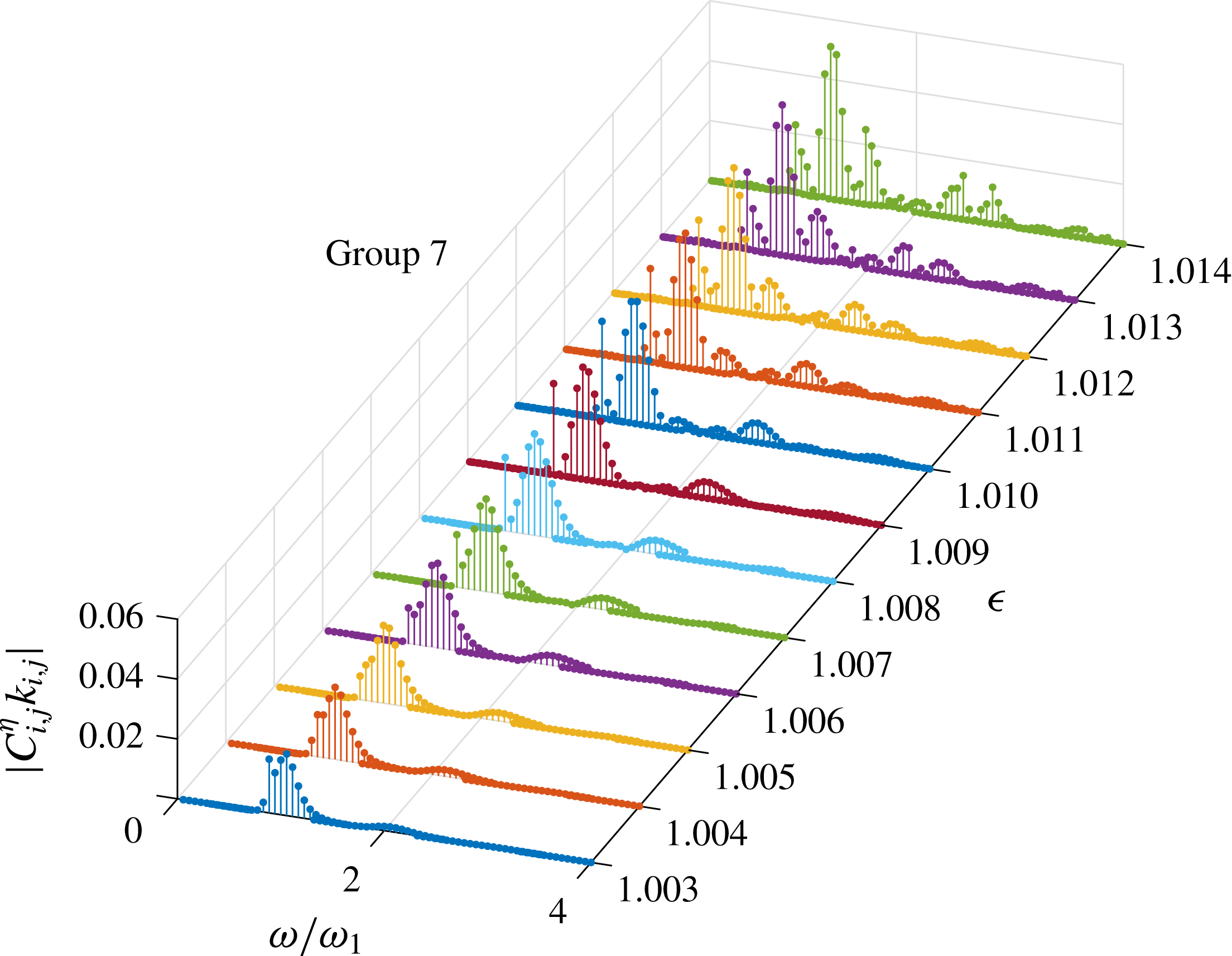
The same as figure 5.

More calculations have been carried out for other groups in table 2. In most groups, the spectrum broadens and the asymmetry is more pronounced when the dimensionless frequency
 $\unicode[STIX]{x1D716}$
increases. Only in a few groups does the energy shrink to one or two components. Taking the first group in figure 3 (group 7) as an example, the amplitude spectra in figure 6 show that the number of components joining the near resonance increases considerably with
 $\unicode[STIX]{x1D716}$
. At
 $\unicode[STIX]{x1D716}=1.014$
, the wave steepness reaches
 $H_{steepness}=0.26$
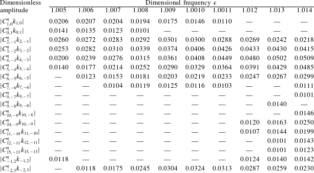
. The wave energy is mainly contained by the components between the first-order primary components and the second-order bound ones. No spectral symmetry is found. The components together with the related coefficients in the initial potential (2.46) are shown in table 7 in appendix B, and the dimensionless amplitudes of the components with
 $|C_{i,j}^{\unicode[STIX]{x1D702}}k_{i,j}|>0.01$
are shown in table 11 in appendix D.
Detailed components together with the related coefficients in the initial guess (2.46) for different dimensionless frequencies
 $\unicode[STIX]{x1D716}$
in group 5, for angle
 $\unicode[STIX]{x1D6FC}=\unicode[STIX]{x03C0}/36$
, wavenumber ratio
 $\unicode[STIX]{x1D70F}=0.89$
and
 $k_{2}=\unicode[STIX]{x03C0}/5$
.

Detailed components together with the related coefficients in the initial guess (2.46) for different dimensionless frequencies
 $\unicode[STIX]{x1D716}$
in group 6, for angle
 $\unicode[STIX]{x1D6FC}=\unicode[STIX]{x03C0}/36$
, wavenumber ratio
 $\unicode[STIX]{x1D70F}=0.89$
and
 $k_{2}=\unicode[STIX]{x03C0}/5$
.

The spectra in figures 5 and 6 illustrate that the auxiliary linear operator (2.38) and the initial guess (2.46) proposed in (§ 2.3) work well for multiple near resonances. Small divisors are indeed resolved when more components join the resonance. Theoretically, no limit is set on the number of components joining the near resonance, and it is reasonable to predict the existence of larger-amplitude steady-state wave groups until the waves break.
4 Concluding remarks
Exactly nonlinear water wave equations are solved in the framework of the HAM to gain finite amplitude wave groups with time-independent spectra when the resonance criterion is nearly satisfied.
The HAM-based approach does not depend on small physical parameters, so no assumption is made about the number or the amplitude of the wave components. For that reason, the present work yields convergent high-order approximation solutions when the nonlinearity of the wave group increases. A piecewise parameter is introduced into the linear operator to transform the small divisors associated with non-trivial nearly resonant components to the singularities associated with exactly resonant ones. Primary exactly resonant and nearly resonant components are considered as initial non-trivial components since all of them are homogeneous solutions to the linear operator. Up to 14 non-trivial components are considered in the initial guess for finite amplitude wave groups.
Small-amplitude wave groups are considered first. The continuum of steady-state resonance in wavevector space is confirmed and the energy transfer between nearby nearly resonant components is identified. As the nonlinearity increases, more components join the near resonance so the frequency broadening and spectral asymmetry are more pronounced. The increased number of solutions with respect to the nonlinearity reveals that the probability of wave components with constant amplitudes and frequencies forming a time-independent spectrum is higher than ever thought. The amplitude of each component may increase or decrease, whereas the amplitude of the whole wave group increases continuously with the nonlinearity. Finite amplitude wave groups with steepnesses of no less than
 $0.21$
are obtained. The wave energy is mainly contained by components near the first-order primary components, with some by second-order bound ones.
This paper confirms the existence of steady-state wave groups with multiple near resonances. The finite amplitude steady-state wave groups obtained would serve as a benchmark for long-time nonlinear wave evolution, e.g. using fully nonlinear solutions methods that exist and are currently in use. It is difficult to generate all of the components in a steady-state resonant wave group experimentally, but we would capture the time-independent spectrum if the small-amplitude components ignored have little impact on the spectral evolution. Taking the steady-state resonant wave groups that are formed by several short-crested waves as an example, the existence of steady-state resonant waves has been confirmed by laboratory experiments in a deep wave basin (Liu et al. Reference Liu, Xu, Li, Peng, Alsaedi and Liao2015). To investigate the long-time propagation of steady-state resonant wave groups, experimental work on collinear steady-state resonant wave groups propagating in a towing tank is underway.
Detailed components together with the related coefficients in the initial guess (2.46) for different dimensionless frequencies
 $\unicode[STIX]{x1D716}$
in group 7, for angle
 $\unicode[STIX]{x1D6FC}=\unicode[STIX]{x03C0}/36$
, wavenumber ratio
 $\unicode[STIX]{x1D70F}=0.89$
and
 $k_{2}=\unicode[STIX]{x03C0}/5$
.

Traditionally, it is widely believed that nearly resonant wave interactions are unsteady. This is true in general cases. However, this work indicates that, in some special cases, the interactions of nearly resonant waves can be steady state, i.e. the spectrum can remain unchanged with time. This is the same as the interactions of exactly resonant waves, which can be steady-state in some special cases, as indicated by the theoretical and experimental work of Xu et al. (Reference Xu, Lin, Liao and Stiassnie2012), Liu & Liao (Reference Liu and Liao2014), Liu et al. (Reference Liu, Xu, Li, Peng, Alsaedi and Liao2015) and Liao et al. (Reference Liao, Xu and Stiassnie2016). We note that in real oceanic conditions, the spectral evolution in infinite depth depends not only on nonlinear interactions, but also on wind input and dissipation due to breaking, which are not considered here.
Acknowledgements
The authors are grateful to the anonymous reviewers for their valuable comments and suggestions which enhanced the quality of this article. This work was partly supported by the National Natural Science Foundation of China (Approval nos 51609090, 11602136 and 11432009) and a science research project of Huazhong University of Science
 $\&$
Technology (Approval nos 0118140077 and 2006140115).
Appendix A. Definitions of
 $\unicode[STIX]{x1D6E5}_{m}^{\unicode[STIX]{x1D702}}$
and
$\unicode[STIX]{x1D6E5}_{m}^{\unicode[STIX]{x1D711}}$
in (2.16) and (2.17)


The definitions of
 $\unicode[STIX]{x1D6E5}_{m}^{\unicode[STIX]{x1D702}}$
and
 $\unicode[STIX]{x1D6E5}_{m}^{\unicode[STIX]{x1D711}}$
in (2.16) and (2.17) are given by
 $$\begin{eqnarray}\displaystyle & \displaystyle \unicode[STIX]{x1D6E5}_{m}^{\unicode[STIX]{x1D702}}=\unicode[STIX]{x1D702}_{m}-{\displaystyle \frac{1}{g}}(\unicode[STIX]{x1D70E}_{1}\bar{\unicode[STIX]{x1D711}}_{m}^{1,0}+\unicode[STIX]{x1D70E}_{2}\bar{\unicode[STIX]{x1D711}}_{m}^{0,1}-\unicode[STIX]{x1D6E4}_{m,0}), & \displaystyle\end{eqnarray}$$
 $$\begin{eqnarray}\displaystyle & \displaystyle \unicode[STIX]{x1D6E5}_{m}^{\unicode[STIX]{x1D711}}=\unicode[STIX]{x1D70E}_{1}^{2}\bar{\unicode[STIX]{x1D711}}_{m}^{2,0}+2\unicode[STIX]{x1D70E}_{1}\unicode[STIX]{x1D70E}_{2}\bar{\unicode[STIX]{x1D711}}_{m}^{1,1}+\unicode[STIX]{x1D70E}_{2}^{2}\bar{\unicode[STIX]{x1D711}}_{m}^{0,2}+g\bar{\unicode[STIX]{x1D711}}_{z,m}^{0,0}-2(\unicode[STIX]{x1D70E}_{1}\unicode[STIX]{x1D6E4}_{m,1}+\unicode[STIX]{x1D70E}_{2}\unicode[STIX]{x1D6E4}_{m,2})+\unicode[STIX]{x1D6EC}_{m}, & \displaystyle\end{eqnarray}$$
where
 $$\begin{eqnarray}\displaystyle \unicode[STIX]{x1D6E4}_{m,0} & = & \displaystyle {\displaystyle \frac{k_{1}^{2}}{2}}\displaystyle \mathop{\sum }_{n=0}^{m}\bar{\unicode[STIX]{x1D711}}_{n}^{1,0}\bar{\unicode[STIX]{x1D711}}_{m-n}^{1,0}+\boldsymbol{k}_{1}\boldsymbol{\cdot }\boldsymbol{k}_{2}\displaystyle \mathop{\sum }_{n=0}^{m}\bar{\unicode[STIX]{x1D711}}_{n}^{1,0}\bar{\unicode[STIX]{x1D711}}_{m-n}^{0,1}+{\displaystyle \frac{k_{2}^{2}}{2}}\displaystyle \mathop{\sum }_{n=0}^{m}\bar{\unicode[STIX]{x1D711}}_{n}^{0,1}\bar{\unicode[STIX]{x1D711}}_{m-n}^{0,1}\nonumber\\ \displaystyle & & \displaystyle +\,{\displaystyle \frac{1}{2}}\displaystyle \mathop{\sum }_{n=0}^{m}\bar{\unicode[STIX]{x1D711}}_{z,n}^{0,0}\bar{\unicode[STIX]{x1D711}}_{z,m-n}^{0,0},\end{eqnarray}$$
 $$\begin{eqnarray}\displaystyle \unicode[STIX]{x1D6E4}_{m,1} & = & \displaystyle \displaystyle \mathop{\sum }_{n=0}^{m}(k_{1}^{2}\bar{\unicode[STIX]{x1D711}}_{n}^{1,0}\bar{\unicode[STIX]{x1D711}}_{m-n}^{2,0}+k_{2}^{2}\bar{\unicode[STIX]{x1D711}}_{n}^{0,1}\bar{\unicode[STIX]{x1D711}}_{m-n}^{1,1}+\bar{\unicode[STIX]{x1D711}}_{z,n}^{0,0}\bar{\unicode[STIX]{x1D711}}_{z,m-n}^{1,0})\nonumber\\ \displaystyle & & \displaystyle +\,\boldsymbol{k}_{1}\boldsymbol{\cdot }\boldsymbol{k}_{2}\displaystyle \mathop{\sum }_{n=0}^{m}(\bar{\unicode[STIX]{x1D711}}_{n}^{1,0}\bar{\unicode[STIX]{x1D711}}_{m-n}^{1,1}+\bar{\unicode[STIX]{x1D711}}_{n}^{2,0}\bar{\unicode[STIX]{x1D711}}_{m-n}^{0,1}),\end{eqnarray}$$
 $$\begin{eqnarray}\displaystyle \unicode[STIX]{x1D6E4}_{m,2} & = & \displaystyle \displaystyle \mathop{\sum }_{n=0}^{m}(k_{1}^{2}\bar{\unicode[STIX]{x1D711}}_{n}^{1,0}\bar{\unicode[STIX]{x1D711}}_{m-n}^{1,1}+k_{2}^{2}\bar{\unicode[STIX]{x1D711}}_{n}^{0,1}\bar{\unicode[STIX]{x1D711}}_{m-n}^{0,2}+\bar{\unicode[STIX]{x1D711}}_{z,n}^{0,0}\bar{\unicode[STIX]{x1D711}}_{z,m-n}^{0,1})\nonumber\\ \displaystyle & & \displaystyle +\,\boldsymbol{k}_{1}\boldsymbol{\cdot }\boldsymbol{k}_{2}\displaystyle \mathop{\sum }_{n=0}^{m}(\bar{\unicode[STIX]{x1D711}}_{n}^{1,0}\bar{\unicode[STIX]{x1D711}}_{m-n}^{0,2}+\bar{\unicode[STIX]{x1D711}}_{n}^{0,1}\bar{\unicode[STIX]{x1D711}}_{m-n}^{1,1}),\end{eqnarray}$$
 $$\begin{eqnarray}\displaystyle \unicode[STIX]{x1D6E4}_{m,3} & = & \displaystyle \displaystyle \mathop{\sum }_{n=0}^{m}(k_{1}^{2}\bar{\unicode[STIX]{x1D711}}_{n}^{1,0}\bar{\unicode[STIX]{x1D711}}_{z,m-n}^{1,0}+k_{2}^{2}\bar{\unicode[STIX]{x1D711}}_{n}^{0,1}\bar{\unicode[STIX]{x1D711}}_{z,m-n}^{0,1}+\bar{\unicode[STIX]{x1D711}}_{z,n}^{0,0}\bar{\unicode[STIX]{x1D711}}_{zz,m-n}^{0,0})\nonumber\\ \displaystyle & & \displaystyle +\,\boldsymbol{k}_{1}\boldsymbol{\cdot }\boldsymbol{k}_{2}\displaystyle \mathop{\sum }_{n=0}^{m}(\bar{\unicode[STIX]{x1D711}}_{n}^{1,0}\bar{\unicode[STIX]{x1D711}}_{z,m-n}^{0,1}+\bar{\unicode[STIX]{x1D711}}_{n}^{0,1}\bar{\unicode[STIX]{x1D711}}_{z,m-n}^{1,0}),\end{eqnarray}$$
 $$\begin{eqnarray}\displaystyle \unicode[STIX]{x1D6EC}_{m} & = & \displaystyle \displaystyle \mathop{\sum }_{n=0}^{m}(k_{1}^{2}\bar{\unicode[STIX]{x1D711}}_{n}^{1,0}\unicode[STIX]{x1D6E4}_{m-n,1}+k_{2}^{2}\bar{\unicode[STIX]{x1D711}}_{n}^{0,1}\unicode[STIX]{x1D6E4}_{m-n,2}+\bar{\unicode[STIX]{x1D711}}_{z,n}^{0,0}\unicode[STIX]{x1D6E4}_{m-n,3})\nonumber\\ \displaystyle & & \displaystyle +\,\boldsymbol{k}_{1}\boldsymbol{\cdot }\boldsymbol{k}_{2}\displaystyle \mathop{\sum }_{n=0}^{m}(\bar{\unicode[STIX]{x1D711}}_{n}^{1,0}\unicode[STIX]{x1D6E4}_{m-n,2}+\bar{\unicode[STIX]{x1D711}}_{n}^{0,1}\unicode[STIX]{x1D6E4}_{m-n,1}),\end{eqnarray}$$
with the definitions
 $$\begin{eqnarray}\displaystyle & \displaystyle \unicode[STIX]{x1D707}_{m,n}=\left\{\begin{array}{@{}ll@{}}\unicode[STIX]{x1D702}_{n}, & m=1,n\geqslant 1,\\[2.0pt] \displaystyle \mathop{\sum }_{i=m-1}^{n-1}\unicode[STIX]{x1D707}_{m-1,i}\unicode[STIX]{x1D702}_{n-i}, & m\geqslant 2,n\geqslant m,\end{array}\right. & \displaystyle\end{eqnarray}$$
 $$\begin{eqnarray}\displaystyle & \displaystyle \unicode[STIX]{x1D713}_{i,j}^{n,m}={\displaystyle \frac{\unicode[STIX]{x2202}^{i+j}}{\unicode[STIX]{x2202}\unicode[STIX]{x1D709}_{1}^{i}\unicode[STIX]{x2202}\unicode[STIX]{x1D709}_{2}^{j}}}\left({\displaystyle \frac{1}{m!}}\left.{\displaystyle \frac{\unicode[STIX]{x2202}^{m}\unicode[STIX]{x1D711}_{n}}{\unicode[STIX]{x2202}z^{m}}}\right|_{z=0}\right), & \displaystyle\end{eqnarray}$$
 $$\begin{eqnarray}\displaystyle & \displaystyle \unicode[STIX]{x1D6FD}_{i,j}^{n,m}=\left\{\begin{array}{@{}ll@{}}\unicode[STIX]{x1D713}_{i,j}^{n,0}, & m=0,\\[2.0pt] \displaystyle \mathop{\sum }_{s=1}^{m}\unicode[STIX]{x1D713}_{i,j}^{n,s}\unicode[STIX]{x1D707}_{s,m}, & m\geqslant 1,\end{array}\right. & \displaystyle\end{eqnarray}$$
 $$\begin{eqnarray}\displaystyle & \displaystyle \unicode[STIX]{x1D6FE}_{i,j}^{n,m}=\left\{\begin{array}{@{}ll@{}}\unicode[STIX]{x1D713}_{i,j}^{n,1}, & m=0,\\[2.0pt] \displaystyle \mathop{\sum }_{s=1}^{m}(s+1)\unicode[STIX]{x1D713}_{i,j}^{n,s+1}\unicode[STIX]{x1D707}_{s,m}, & m\geqslant 1,\end{array}\right. & \displaystyle\end{eqnarray}$$
 $$\begin{eqnarray}\displaystyle & \displaystyle \unicode[STIX]{x1D6FF}_{i,j}^{n,m}=\left\{\begin{array}{@{}ll@{}}2\unicode[STIX]{x1D713}_{i,j}^{n,2}, & m=0,\\[2.0pt] \displaystyle \mathop{\sum }_{s=1}^{m}(s+1)(s+2)\unicode[STIX]{x1D713}_{i,j}^{n,s+2}\unicode[STIX]{x1D707}_{s,m}, & m\geqslant 1,\end{array}\right. & \displaystyle\end{eqnarray}$$
 $$\begin{eqnarray}\displaystyle & \displaystyle \bar{\unicode[STIX]{x1D711}}_{n}^{i,j}=\displaystyle \mathop{\sum }_{m=0}^{n}\unicode[STIX]{x1D6FD}_{i,j}^{n-m,m}, & \displaystyle\end{eqnarray}$$
 $$\begin{eqnarray}\displaystyle & \displaystyle \bar{\unicode[STIX]{x1D711}}_{z,n}^{i,j}=\displaystyle \mathop{\sum }_{m=0}^{n}\unicode[STIX]{x1D6FE}_{i,j}^{n-m,m}, & \displaystyle\end{eqnarray}$$
 $$\begin{eqnarray}\displaystyle & \displaystyle \bar{\unicode[STIX]{x1D711}}_{zz,n}^{i,j}=\displaystyle \mathop{\sum }_{m=0}^{n}\unicode[STIX]{x1D6FF}_{i,j}^{n-m,m}. & \displaystyle\end{eqnarray}$$
A detailed derivation can be found in appendix A in Liao (Reference Liao2011).
Appendix B. Initial potentials for groups 5, 6 and 7
Detailed components together with the related coefficients in the initial guess (2.46) for different dimensionless frequencies
 $\unicode[STIX]{x1D716}$
in groups 5, 6 and 7 are shown in tables 7, 5 and 6 respectively. Here, the angle
 $\unicode[STIX]{x1D6FC}=\unicode[STIX]{x03C0}/36$
, the wavenumber ratio
 $\unicode[STIX]{x1D70F}=0.89$
and
 $k_{2}=\unicode[STIX]{x03C0}/5$
.
Appendix C. Convergence of series solutions obtained by the HAM for multiple near-resonant wave groups
We define the averaged residual squares
 $\unicode[STIX]{x1D700}_{m}^{\unicode[STIX]{x1D702}}$
and
 $\unicode[STIX]{x1D700}_{m}^{\unicode[STIX]{x1D711}}$
,
 $$\begin{eqnarray}\displaystyle & \displaystyle \unicode[STIX]{x1D700}_{m}^{\unicode[STIX]{x1D702}}={\displaystyle \frac{\unicode[STIX]{x03C0}^{2}}{M^{2}}}\mathop{\sum }_{i=0}^{M}\mathop{\sum }_{j=0}^{M}\left[\displaystyle \mathop{\sum }_{n=0}^{m-1}\unicode[STIX]{x1D6E5}_{n}^{\unicode[STIX]{x1D702}}(i\unicode[STIX]{x0394}\unicode[STIX]{x1D709}_{1},j\unicode[STIX]{x0394}\unicode[STIX]{x1D709}_{2})\right]^{2}, & \displaystyle\end{eqnarray}$$
 $$\begin{eqnarray}\displaystyle & \displaystyle \unicode[STIX]{x1D700}_{m}^{\unicode[STIX]{x1D711}}={\displaystyle \frac{\unicode[STIX]{x03C0}^{2}}{M^{2}}}\mathop{\sum }_{i=0}^{M}\mathop{\sum }_{j=0}^{M}\left[\displaystyle \mathop{\sum }_{n=0}^{m-1}\unicode[STIX]{x1D6E5}_{n}^{\unicode[STIX]{x1D711}}(i\unicode[STIX]{x0394}\unicode[STIX]{x1D709}_{1},j\unicode[STIX]{x0394}\unicode[STIX]{x1D709}_{2})\right]^{2}, & \displaystyle\end{eqnarray}$$
where
 $\unicode[STIX]{x1D6E5}_{n}^{\unicode[STIX]{x1D702}}$
and
 $\unicode[STIX]{x1D6E5}_{n}^{\unicode[STIX]{x1D711}}$
are given in appendix A,
 $M$
is the number of discrete points and
 $\unicode[STIX]{x0394}\unicode[STIX]{x1D709}_{1}=\unicode[STIX]{x0394}\unicode[STIX]{x1D709}_{2}=\unicode[STIX]{x03C0}/M$
. Here,
 $M=5$
is used.
Taking the solutions obtained by the HAM for
 $\unicode[STIX]{x1D716}=1.010$
in group 5 as an example, the averaged residual squares
 $\unicode[STIX]{x1D700}_{m}^{\unicode[STIX]{x1D702}}$
and
 $\unicode[STIX]{x1D700}_{m}^{\unicode[STIX]{x1D711}}$
at different orders of approximation are shown in figure 7. Here, the angle
 $\unicode[STIX]{x1D6FC}=\unicode[STIX]{x03C0}/36$
, the wavenumber ratio
 $\unicode[STIX]{x1D70F}=0.89$
and
 $k_{2}=\unicode[STIX]{x03C0}/5$
. We choose the convergence-control parameter
 $c_{0}=-0.6$
. Figure 8 shows that the two averaged residual squares decrease continuously when the order of approximation increases. The corresponding high-order approximation of unknown constants
 $C_{m,n}^{\unicode[STIX]{x1D702}}$
in (2.11) converges quickly, as shown in table 8. Once the convergence of series solutions is guaranteed, we then use the Padé approximation to accelerate the convergence of the unknown amplitude
 $C_{m,n}^{\unicode[STIX]{x1D702}}$
after the HAM calculations are finished.
Residual squares of
 $\log _{10}\unicode[STIX]{x1D700}_{m}^{\unicode[STIX]{x1D702}}$
and
 $\log _{10}\unicode[STIX]{x1D700}_{m}^{\unicode[STIX]{x1D711}}$
versus
 $c_{0}$
for
 $\unicode[STIX]{x1D716}=1.010$
in group 5, for angle
 $\unicode[STIX]{x1D6FC}=\unicode[STIX]{x03C0}/36$
, wavenumber ratio
 $\unicode[STIX]{x1D70F}=0.89$
and
 $k_{2}=\unicode[STIX]{x03C0}/5$
: solid line, second-order approximation; dashed line, third-order approximation; dotted line, fourth-order approximation; dash–dot line, fifth-order approximation.

Residual squares of
 $\log _{10}\unicode[STIX]{x1D700}_{m}^{\unicode[STIX]{x1D702}}$
and
 $\log _{10}\unicode[STIX]{x1D700}_{m}^{\unicode[STIX]{x1D711}}$
versus the approximation order
 $m$
when
 $c_{0}=-0.6$
for
 $\unicode[STIX]{x1D716}=1.010$
in group 5, for angle
 $\unicode[STIX]{x1D6FC}=\unicode[STIX]{x03C0}/36$
, wavenumber ratio
 $\unicode[STIX]{x1D70F}=0.89$
and
 $k_{2}=\unicode[STIX]{x03C0}/5$
: solid line,
 $\log _{10}\unicode[STIX]{x1D700}_{m}^{\unicode[STIX]{x1D702}}$
; dotted line,
 $\log _{10}\unicode[STIX]{x1D700}_{m}^{\unicode[STIX]{x1D711}}$
.

The
 $m$
th-order approximation of the dimensionless amplitude of components with
 $|C_{ij}^{\unicode[STIX]{x1D702}}k_{ij}|>0.01$
in group 5, for angle
 $\unicode[STIX]{x1D6FC}=\unicode[STIX]{x03C0}/36$
, wavenumber ratio
 $\unicode[STIX]{x1D70F}=0.89$
, dimensionless frequency
 $\unicode[STIX]{x1D716}=1.010$
and
 $c_{0}=-0.6$
.

The dimensionless amplitudes of components with
 $|C_{i,j}^{\unicode[STIX]{x1D702}}k_{i,j}|>0.01$
in steady-state near-resonant waves for different dimensionless frequencies
 $\unicode[STIX]{x1D716}$
in group 5, for angle
 $\unicode[STIX]{x1D6FC}=\unicode[STIX]{x03C0}/36$
and wavenumber ratio
 $\unicode[STIX]{x1D70F}=0.89$
.

The dimensionless amplitudes of components with
 $|C_{i,j}^{\unicode[STIX]{x1D702}}k_{i,j}|>0.01$
in steady-state near-resonant waves for different dimensionless frequencies
 $\unicode[STIX]{x1D716}$
in group 6, for angle
 $\unicode[STIX]{x1D6FC}=\unicode[STIX]{x03C0}/36$
and wavenumber ratio
 $\unicode[STIX]{x1D70F}=0.89$
.

The dimensionless amplitudes of components with
 $|C_{i,j}^{\unicode[STIX]{x1D702}}k_{i,j}|>0.01$
in steady-state near-resonant waves for different dimensionless frequencies
 $\unicode[STIX]{x1D716}$
in group 7, for angle
 $\unicode[STIX]{x1D6FC}=\unicode[STIX]{x03C0}/36$
and wavenumber ratio
 $\unicode[STIX]{x1D70F}=0.89$
.

Appendix D. Surface elevations in groups 5, 6 and 7
The dimensionless amplitudes of components with
 $|C_{i,j}^{\unicode[STIX]{x1D702}}k_{i,j}|>0.01$
in steady-state nearly resonant waves for different dimensionless frequencies
 $\unicode[STIX]{x1D716}$
in groups 5, 6 and 7 are shown in tables 9–11 respectively. Here, the angle
 $\unicode[STIX]{x1D6FC}=\unicode[STIX]{x03C0}/36$
and the wavenumber ratio
 $\unicode[STIX]{x1D70F}=0.89$
.