

Introduction
The literature pertaining to the effects of early life stressors on later life health includes opposing theoretical mechanisms. Some literature suggests that stressful perinatal environments cause excess morbidity in later life,Reference Ben-Shlomo and Kuh 1 , Reference Barker 2 , Reference Gluckman, Hanson, Beedle and Raubenheimer 3 while competing literature posits that adverse perinatal environments ‘cull’ cohorts of less robust members and leave survivors who, on average, live longer than those in other cohorts.Reference Catalano 4 , Reference Störmer 5
A relatively smaller body of literature argues that early adolescence (approximately ages 10–14) may also present opportunities for threatening environments to affect developmental trajectories and health later in life,Reference Kuh and Ben-Shlomo 6 , Reference Crone and Dahl 7 although the theoretical mechanism explaining this phenomenon remains less explored. Early adolescence encompasses a particularly important interval in which the onset of puberty results in a cascade of physical, emotional, cognitive and social changes.Reference Crone and Dahl 7 Environmental threats during this time may, however, result in a tradeoff of longevity for reproductive success.Reference Ellis, Boyce, Belsky, Bakermans-Kranenburg and van Ijzendoorn 8 , Reference Selevan, Kimmel and Mendola 9
An evolutionary perspective suggests that a perceived threat among male adolescents may trigger physiological responses, such as earlier onset of puberty and accelerated growth that increase their likelihood of attaining reproductive success.Reference Ellis, Del Giudice and Dishion 10 Changes in gonadal hormone levels may also affect adolescents’ propensity to take risks, which appears to be motivated, at least in part, by adolescents’ inclination to acquire social status.Reference Crone and Dahl 7 Such adaptations may have improved fitness over the course of human evolution, but may come at the expense of later life morbidity or premature mortality in contemporary populations.Reference Dodge and Albert 11
Two studies report findings consistent with the argument that a stressful early adolescence adversely affects male longevity. One study found that the cohort of males who were in adolescence (approximately age 15) in Germany during World War I experienced higher death rates at middle age compared to preceding or succeeding cohorts.Reference Horiuchi 12 The author attributed this difference, which peaked in cohorts born between 1899 and 1904, to the stressful effects of World War I (e.g. malnutrition) on young males in general and on adolescents in particular. A second study reports that among males conscripted to military service in Sweden from 1949 to 1951, low-ranking parental occupation at age 9–11 predicted elevated risk of coronary heart disease in middle age.Reference Falkstedt, Lundberg and Hemmingsson 13 While consistent with evidence suggesting adolescence as a sensitive period, both findings employ weak tests of association and use temporally limited samples.
The underlying theory does not exclude effects on women.Reference Catalano 4 Female adolescents also experience somatic adaptations in response to environmental threats, although their response appears more physiological than behavioral.Reference Ellis, Del Giudice and Dishion 10 , Reference Belsky, Steinberg, Houts and Halpern-Felsher 14 Evidence suggests an association between environmental threats, in the form of high extrinsic mortality (i.e. risk of death not conditional on an individual’s behavior), and delayed puberty and timing of menarche.Reference Gluckman and Hanson 15 Theory predicts that this delay occurs during stressful times so that females may preserve somatic resources either for self-preservation or in expectation of better times in the future.Reference Placek and Quinlan 16 The implications of this theory for longevity remain unexplored.
Given evidence suggesting that the stress response during adolescence appears sex dependent, we contribute to the literature by testing the hypothesis that life span from age 20 among male birth cohorts unambiguously exposed to life-threatening stressors during early adolescence will fall below that among other males. We test the hypothesis among males born in France between 1816 and 1919, England and Wales between 1841 and 1919, and Sweden from 1861 to 1919. We control for trends, cycles and other forms of autocorrelation in life span from age 20, and for exposure to life-threatening stressors at infancy, childhood and late adolescence.
Methods
Variables and data
We used sex-specific cohort life expectancy at age 20 (i.e. average life span from age 20 in annual birth cohorts) as our dependent variable, given that the elaboration of reproductive biology and related accommodation of the soma (i.e. non-reproductive biology) is completed by that age.
The literature arguing for sensitive or critical developmental periods assumes that populations exposed to unusual threats to health at ages specified a priori will suffer earlier mortality than other populations. Following this literature, we define the period of early adolescence as age 10–14.Reference Ellis, Del Giudice and Dishion 10 , Reference Cameron and Demerath 17 , Reference Spear 18 We use age- and sex-specific mortality rates as our independent and control variables. More specifically, we use the male infant mortality rate, as well as male mortality rates from ages 1–4, 5–9, 10–14 and 15–19, as predictors of male cohort life expectancy at age 20. Results would support the argument that adversity in early adolescence affects later life health if mortality rates in the age group 10–14 inversely predict cohort life expectancy at age 20.
We obtained age- and sex-specific cohort life expectancy and death rates from the Human Mortality Database. 19 This archive includes life table data that meet quality standards agreed among demographers and other population researchers. Few societies have kept reliable vital statistics from which we can calculate cohort life expectancy over long periods of time. Three societies that have such data, France, England and Wales, and Sweden, differ in the frequency of societal disruption by war – a phenomenon that could, by inducing high period mortality among young males, obscure other causes of differences in life span among birth cohorts. Sweden, which has kept reliable vital statistics since 1861, provides an opportunity to test our hypothesis in society with relatively few wars. France, which has reliable data dating to 1816, allows a test in a society with a history of more hostilities, while England and Wales, with data beginning in 1841, fall between the two. We used the total Swedish population and the civilian populations of France as well as England and Wales.
By axiom, demographers can calculate cohort life expectancy only among birth cohorts whose members have all, or nearly all, died. The time series described below, therefore, ends with cohorts born in 1919.
Analyses
Correlational tests essentially determine whether the observed values of two variables differ, as predicted by theory, from their statistically expected values in the same cases. Such tests typically assume that the statistically expected value of each variable equals its mean. Time series, however, often exhibit ‘autocorrelation’ in the form of trends, cycles and the tendency to remain elevated or depressed after high or low values. These patterns complicate correlational tests because the expected value of a patterned series is not its mean. No one, in other words, would predict the future values of a series to be its mean if past values of the series exhibited autocorrelation.
Researchers often solve the autocorrelation problem through the purely empirical approach of identifying patterns in a time series and expressing them as a product of earlier behavior in the series. Time-series equations used to test hypotheses, therefore, often include ‘lags’ of the dependent variable among predictor variables.
Our test turns on whether male cohort life expectancy at age 20 falls below its statistically expected value in cohorts that exhibited higher mortality rates at ages 10–14 than their statistically expected values. We arrived at the statistically expected values of our independent and dependent variables via the methods conceived by FisherReference Fisher 20 and developed by Box and Jenkins.Reference Box, Jenkins and Reinsel 21 More specifically, our test proceeded through the following steps:
-
1. We used the strategy developed by Box and JenkinsReference Box, Jenkins and Reinsel 21 to identify and model autocorrelation in male cohort life expectancy, measured in months, at age 20 in France (1816–1919), England and Wales (1841–1919), and Sweden (1861–1919). This strategy identifies which of a large family of mathematical expressions best describes measurements made serially in time or space. Metaphorically, the modeling procedure assumes that the measurements passed through an unobserved ‘filter’ that imposed autocorrelation upon them. The procedure uses mathematical ‘signatures’ to narrow the likely filters to a few and then applies estimates of ‘fit’Reference Ljung and Box 22 to identify the most likely candidate. The differences between the values predicted by the model and the observed series approximate the values that passed through the filter. They meet the assumptions of traditional tests of association because they are independent of each other (i.e. exhibit no autocorrelation), their expected value equals their mean (i.e. 0) and they exhibit constant variability over time.
-
2. We applied the Box and Jenkins routines described above to male infant mortality rates and to male mortality rates at age 1–4, 5–9, 10–14 and 15–19 in each of the three societies for the years listed above. We expressed all as cohort mortality rates per 1000 persons at risk.
-
3. We estimated the equation formed by adding the residuals of the five age-specific mortality series to the equation resulting from step 2. This specification yields the following general test equation.
 $$\eqalignno{ & \nabla Y_{t} ={\rm \romega }_{1} \nabla X_{{0t}} {\plus}{\rm \romega }_{2} \nabla {X}_{{{\rm 1{-}4}t}} {\plus}{\rm \romega }_{3} \nabla {X}_{{{\rm 5{-}9}t}} {\plus}{\rm \romega }_{4} \nabla {X}_{{{\rm 10{-}14}t}} \cr & {\plus}{\rm \romega }_{{5}} \nabla {X}_{{{\rm 15{-}19}t}} {\plus}{{\left( {1{\minus}{\rm \rtheta }_{{\rm 1}} B{\minus}{\rm \rtheta }_{2} B^{{\rm 2}} {\minus}\,\ldots\,{\minus}{\rm \rtheta }qB^^{q} } \right)} \over {\left( {1{\minus}{\rm \rphi }_{{\rm 1}} B{\minus}{\rm \rphi}_{2} B^{{\rm 2}} {\minus}\,\ldots\,{\minus}{\rm \rphi }pB^^{p} } \right)}}a_{t} $$
Yt is male cohort life expectancy at age 20, in months, at year t for France, England and Wales, or Sweden.
 $\nabla\!_{d} $
is the difference operator indicating that Y has been differenced (i.e. cohort life expectancy at year t subtracted from that at year t−1). X
0t
–X
15–19t
are the residuals of the best fitting Box–Jenkins models of the male-specific cohort mortality rate (per 1000) at infancy, age 1–4, 5–9, 10–14 and 15–19. ω1–ω5 are the estimated coefficients for the age- and sex-specific death rate residuals. θ is the moving average, or ‘short memory,’ parameter. ϕ is the autoregressive, or ‘long memory,’ parameter. B indicates that either θ or ϕ acts on the value of the error term ‘a’ at year t–q or t–p, and at
is the error term at year t.
The data from France, England and Wales, and Sweden would support our hypotheses if ω4 were significantly greater than 0.
Results
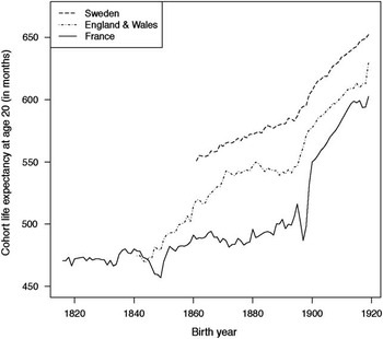
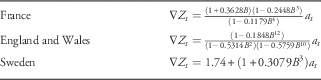
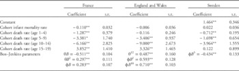
Figure 1 shows cohort life expectancy (in months) for males at age 20 for France, England and Wales, and Sweden. Step 1 in our analyses yielded Box–Jenkins equations, shown in Table 1, from which we derived the expected value of the series shown in Fig. 1.
Observed male cohort life expectancy at age 20 (in months) in France (1816–1919), England and Wales (1841–1919), and Sweden (1861–1919).

Box–Jenkins equations for cohort life expectancy (in months) for males at age 20 for France (1816–1919), England and Wales (1841–1919), and Sweden (1861–1919)

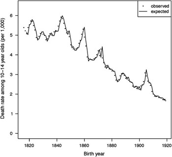
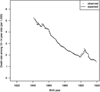
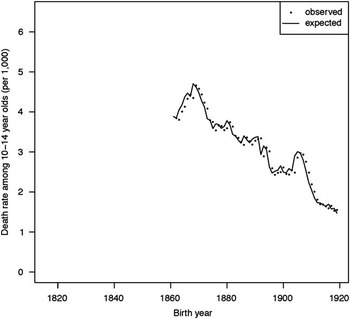
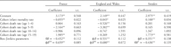
Step 2 required building 15 models for the permutations of five age groups and three societies. The models are shown in a Supplementary appendix available from the authors. As might be expected, these models show a downward trend in mortality rates over time, with varying short-term memory parameters. We describe three models here in detail as an example. Figures 2, 3 and 4 show the expected and observed mortality rate (per 1000) for French, English and Welsh, and Swedish 10–14-year-old males. Table 2 shows the Box–Jenkins models that best fit each of these series.
Observed and expected cohort death rates among males aged 10–14 years in France (1816–1919).

Observed and expected cohort death rates among males aged 10–14 years in England and Wales (1841–1919).

Observed and expected cohort death rates among males aged 10–14 years in Sweden (1841–1919).

Box–Jenkins equations for cohort death rates (per 1000) for males at age 10–14 for France (1816–1919), England and Wales (1841–1919), and Sweden (1861–1919)

The difference operator,
 $\nabla $
, in each of these models expresses the general downward trend in the early adolescent death rate. The autoregressive parameter (i.e. 0.377; s.e.=0.091) in the model for French data, for example, suggests that high or low values carry into succeeding years but decrease geometrically.
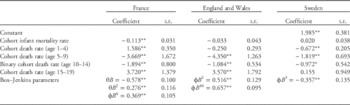
Table 3 shows the results of step 3 in our test. The three significant (P<0.05; two-tailed test), negatively signed coefficients for mortality among 10–14-year-old males support our hypothesis. Cohort life span from age 20 among males varies inversely with mortality in early adolescence in the three societies with the longest, most reliable data. Our use of Box–Jenkins methods implies that this association cannot arise from shared trends, cycles or other forms of autocorrelation. It also cannot logically arise from endogenous cohort frailty that would cause both adolescents and adults to die more frequently in some cohorts than in others. Endogenous cohort frailty would manifest at other ages under 20, thereby keeping any from sharing unique variance with post-age 20 life span.
Coefficients and standard errors for predictors of male cohort life expectancy at age 20 (in months) in France (1816–1919), England and Wales (1841–1919), and Sweden (1861–1919)

*P<0.05, one-tailed test; **P<0.01, one-tailed test.
We show standard errors in Table 3 to give a sense of the stability of coefficients over the birth cohorts, but also remind readers that we have not sampled births for our study. Because our data include all persons recorded as born in France, England and Wales, and Sweden, our coefficients equal – rather than approximate,– the associations over the test period.
Table 4 shows the results of repeating our tests for females, for whom our theory makes no directional prediction. We found no significant associations for early adolescence in any of the three societies.
Coefficients and standard errors for predictors of female cohort life expectancy at age 20 in France (1816–1919), England and Wales, and Sweden

*P<0.05, one-tailed test; **P<0.01, one-tailed test.
We conducted several additional tests to give us a sense of the robustness of our findings. We excluded all variables that were not at least twice their standard errors and estimated the pared equations. Results of the tests remained essentially the same.
We used the methods of Chang et al. Reference Chang, Tiao and Chen 23 to correct our coefficients for outlying sequences of values in the cohort life expectancy variable that could reflect the effect of wars and other ‘shocks’ to male longevity after age 20. The correction adjusts for single-year ‘spikes,’ temporary changes that begin with an outlying value and then regress back over several years to the level expected before the first outlier in the sequence, and sequences that begin with an outlying value but do not decay before the end of the series or return to expected values abruptly without significant decay between the first and last outlier in the sequence. As expected, France exhibited the most (six) outliers, England and Wales fewer (three), and Sweden none. Adjusting for the detected outliers did not change the results of our test.
The coefficients shown in Table 3 convey that life span post-age 20 among male birth cohorts in France, England and Wales, and Sweden over the test period, decreased by 6.17, 9.00 and 3.96 months, respectively, for each increase of one per 1000 in age 10–14 cohort death rates. To help put these statistical statements in context, we transformed the continuous variable for adolescent death rates into a binary score of 1 for cohorts with greater than expected death rates during ages 10–14 and 0 otherwise, and estimated our test equations again. Table 5 shows the results. The coefficient for the binary variable equals average life span lost, in months, after age 20 for male birth cohorts were subjected to higher than expected threats to survival in adolescence. The coefficient for France suggests that males from cohorts highly threatened in adolescence lost 1.9 months of life. Cohort life expectancy at age 20 for French males increased from 456.84 to 602.64 months, an average of 1.4 months a year over the 104 years of this study. Males in our threatened adolescent cohorts therefore lost more life after age 20 (i.e. 1.9 months) than the modernization of French society conferred on all men of their age each year (i.e. 1.4 months) over the test period (i.e. 1816–1919). Applying this logic to England and Wales yields the estimate that men from birth cohorts unusually threatened in adolescence lost 1.1 months of post-age 20 life, while life span for that group increased on average 2 months each year (i.e. from 469.1 to 630.1 months) from 1841 to 1919. The calculation for Sweden shows that while post-age 20 life span among males increased from 550.8 to 652.4 months, or an average of 1.7 months a year from 1861 to 1919, threatened adolescent males lost 0.97 months or more than half the gain, attributable to modernization.
Coefficients and standard errors for predictors of male cohort life expectancy at age 20 in France, England and Wales, and Sweden

Cohort death rate at age 10–14 scored 1 for years when observed values exceeded expected value.
*P<0.05, one-tailed test; **P<0.01, one-tailed test.
Other statistical expressions of this association include the portion of the variance ‘explained’ by our test equations (i.e. R 2) that appears attributable to the death rate at age 10–14. Our test equation for France, for example, accounted for 34.2% of variance in differenced post-age 20 life span, but that estimated decreased to 30.5% when we excluded the age 10–14 death rate. Excluding the early adolescent death rate from the equation for England and Wales decreased the explained variance from 44.6 to 36.7%. Doing the same for Sweden decreased the value from 33.5 to 25.2%.
Discussion
Our findings support the argument that early adolescence is a sensitive developmental period among males. Population stressors experienced during ages 10–14 are more strongly associated with a decrease in life span compared with those experienced during infancy, ages 1–4, 5–9 and 15–19.
Individual health records recording first menstruation suggest a secular trend toward an earlier age of puberty among females. We know of no comparable medical evidence for males, although historical data of symptoms associated with puberty suggest a similar trend among males.Reference Goldstein 24 A study of voice changes, which occur at mid-puberty among males,Reference Lifshitz 25 reports that boys in J.S. Bach’s choirs from 1727–1749 experienced a voice change between the ages of 17 and 18. In comparison, London boys in 1959 experienced the voice change at an average of 13.3 years.Reference Daw 26 This evidence would suggest that males in nineteenth-century Europe experienced mid-puberty between the ages of 14 and 16 and began experiencing the first stages of puberty about 2 years earlier given that pubertal development in males spans several years.Reference Mashall and Turner 27
Adolescent plasticity, or the ability to make physiological and behavioral adaptations in response to environmental stressors, allowed some French, English and Welsh, and Swedish males to survive and reproduce while others died.Reference Dufty, Clobert and Møller 28 , Reference Hochberg, Feil and Constancia 29 Our findings demonstrate, however, that adaptations triggered during adolescence in stressed cohorts came at the expense of reduced life span at age 20. Although research has provided support for such ‘culling’ in utero,Reference Catalano and Bruckner 30 our findings suggest that it does not apply to male adolescents. The results indicate, however, the 5–9 year age group as another potentially sensitive developmental periods among males. While our theory does not predict this sensitive period, it does not logically exclude it either.
Mortality does not occur randomly in populations, even those of the same age and sex. Various factors, such as low socio-economic status or population density, for example, likely predict which adolescents most likely died when nineteenth-century populations suffered exogenous shocks.Reference Razzell and Spence 31 , Reference Preston and Haines 32 The same factors may also have predicted who died early among those in shocked adolescent cohorts who survived to age 20. Historical data available for multiple societies over long periods, do not, however, include sufficient detail to allow us to test suspicions of subgroup differences.
We cannot know which mechanism or mechanisms induced premature mortality in our relatively stressed cohorts. Some research has demonstrated that stressful social circumstances during youth predict uptake of behavioral risk factors for disease, such as smoking and high body mass index.Reference Falkstedt, Lundberg and Hemmingsson 13 Other research, however, suggests that such risk factors were prevalent only among wealthy men and women – at least until the twentieth century.Reference Razzell and Spence 31 Further research linking health behaviors and mortality in nineteenth-century Europe, particularly by sex and socio-economic class, may help explain the phenomenon observed in our results.
Selective migration certainly affected mortality over time in nineteenth-century European populations. We, however, do not think such migration poses a parsimonious rival to our theory. Such migration could have spuriously induced our results only if the likelihood of relatively healthy males (but not females) migrating from France, England and Wales, and Sweden after age 20 varied positively with the death rate of their birth cohort at age 10–14 (but not at ages 1–4 or 15–19). We know of no theory or data that would lead us to suspect such a circumstance.Reference Hatton and Williamson 33
The current study contributes to the existing literature in two ways. First, we use empirical evidence to demonstrate that the period of early adolescence, much like the perinatal period, is a sensitive period for male development. Second, our findings suggest that cohort effects can significantly impact sex-specific mortality trends well into adulthood. Population stressors that affect male adolescents should be taken into account when forecasting or explaining their adult mortality trends. Our results suggest, moreover, that current emphases on early life interventions may be less informed than intuition suggests. Greater resources and attention may need to be devoted to adolescent development given that it also presents as great an opportunity for population stressors to adversely affect human health.
Acknowledgments
None.
Financial Support
This work was supported by the Robert Wood Johnson Foundation Health and Society Scholars Program and the National Institute of Child Health & Human Development (grant # HD07275).
Conflicts of Interest
None.