INTRODUCTION
Marine artificial reef studies commonly refer to the distinction between resident and non-resident species (e.g. D'Anna et al., Reference D'Anna, Badalamenti, Gristina and Pipitone1994; Johnson et al., Reference Johnson, Barnett, DeMartini, Craft, Ambrose and Purcell1994; Moreno, Reference Moreno2002; Jan et al., Reference Jan, Liu, Chen, Wang, Song, Lin and Shao2003). Beyond traditional community monitoring, the core species-transient species distinction appears essential to performance assessment of these objects generally deployed either for fishery purposes or environmental mitigation (Ambrose, Reference Ambrose1994; Caselle et al., Reference Caselle, Love, Fusaro and Schroeder2002). In both cases, specific species are generally targeted (commercially valuable species on the one hand and species particularly affected by environmental damages on the other), and the implications are very different if they are present along the deployed artificial habitat as resident species or as vagrant species.
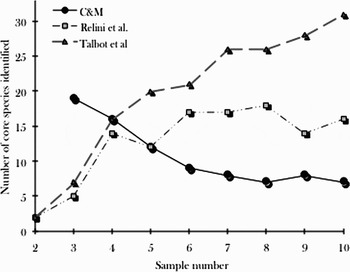
Artificial reef scientists commonly refer to the site fidelity level to distinguish core from transient species. In spite of this, a widely accepted distinction method is still lacking, and there is even no consensus with regard to the number of subdivisions in artificial reef communities. For instance, Talbot et al. (Reference Talbot, Russel and Anderson1978) propose two (resident and transient species), Bohnsack & Talbot (Reference Bohnsack and Talbot1980) chose three (resident, transient and visitor), while Stephens et al. (Reference Stephens, Morris, Pondella, Koonce and Jordan1994) distinguish four different groups (resident, seasonal, transient and rare). Furthermore, despite the fact that the indicators used by different authors are generally all related to site fidelity, they all differ because thresholds between groups are generally set up subjectively. For instance, Talbot et al. (Reference Talbot, Russel and Anderson1978) consider that a species recorded in at least two successive samples may be classified as resident, while Relini et al. (Reference Relini, Torchia and Relini1994) establish as resident the species that appear in at least 50% of the samples, and Costello & Myers (Reference Costello and Myers1996) classify a species as resident only if it is present in all the samples but two. The absence of a theoretical justification makes the evaluation of these different criteria particularly difficult, as they are based on personal choices. Moreover, they usually generate different outputs that are hardly comparable (Figure 1). As a result, we believe that an objective distinction method would constitute an important practical advancement in the field.
Three different distinction criteria applied to an Australian artificial reef dataset. The dataset used was published by Branden et al. (Reference Branden, Pollard and Reimers1994). The three methods represented are taken from Costello & Myers (Reference Costello and Myers1996), Relini et al. (Reference Relini, Torchia and Relini1994) and Talbot et al. (Reference Talbot, Russel and Anderson1978).

Among the few prior theoretical attempts to provide an objective solution, the work published by Magurran & Henderson (Reference Magurran and Henderson2003) is especially valuable with regard to this objective for three main reasons: first, it shows that any community can objectively be decomposed into two groups: core (or resident) and transient species. Second, contrary to Hanski (Reference Hanski1982), Tokeshi (Reference Tokeshi1992), and most of the previous studies related to the core-satellite theory, the authors propose a distinction method which is not based on spatial data but on temporal data. Temporal data represent a type commonly used among artificial habitat scientists, who generally focus on a unique site. Third, Magurran & Henderson (Reference Magurran and Henderson2003) provide four practical methods to distinguish core from transient species: (1) plotting maximum abundance against persistence; (2) fitting a Poisson process to the species occurrence patterns; (3) referring to the species' biological characteristics; and (4) calculating the reciprocal form of the Simpson index (D) for each persistence level species group and looking at its relation with sample size.
However, some potential problems exist: first Magurran & Henderson's purpose was mainly theoretical, rather than practical. Second, the study did not aim for the accurate detection of the boundary between intra-community groups but instead, it focused on explaining the ‘excess of rare species’ usually noticed in species abundance distributions as a result of an overlap between two distributions: a log normal (core species) and a log-series (transient species). Third, we should point out that the dataset used was extremely unusual (a 21-year-long time-series on fish assemblage in an English estuary), and that artificial reef scientists or managers usually face much more modest datasets. For these reasons, it is worth testing the value of such detection tools with regard to particular case studies.
This paper does not aim to assess the general value of these tools proposed and used successfully by Magurran & Henderson (Reference Magurran and Henderson2003) when dealing with any artificial habitat but simply aims to highlight the practical value of these four distinction tools when specifically applied to artificial reef communities. Toward this purpose, we selected four different fish assemblage datasets related to four different artificial reefs. By using highly different cases (regarding to sampling effort, reef structure type, location and even sampling method), we wish to determine if Magurran & Henderson's tools may be suitable for all cases.
MATERIALS AND METHODS
Materials
We used four different datasets. Three of them were drawn from the literature: (1) a reef made up of concrete pipes, deployed off California (hereafter Californian reef) and sampled seasonally during two consecutive years (N = 7) by underwater visual surveys; (2) a reef constructed from discarded tires, deployed off Glenelg (Australia—hereafter Australian reef) and sampled during 32 consecutive months (N = 10) via underwater visual surveys; (3) a steel artificial reef located in the Sea of Japan, off Nezugaseki (Yamagata Prefecture, Japan—hereafter Yamagata reef) and sampled during five consecutive years (N = 30) by using a video camera system. For further details concerning these three reefs, please refer respectively to Matthews (Reference Matthews1985), Branden et al. (Reference Branden, Pollard and Reimers1994) and Takagi et al. (Reference Takagi, Moriguchi, Kimoto, Arai, Hasuo, Nakamura and Kimura2000). The fourth dataset was directly collected along an artificial reef deployed off Okayama (Seto Inland Sea, Okayama Prefecture, Japan—hereafter Okayama reef). This reef was built by the Japanese company Ocean Construction Co. Ltd (Okayama City, Japan). This is a rectangular-basis construction made up of oyster shells and steel bars whose total volume reaches 20.3 m3. The reef was deployed at the end of December 1998 and lies at a depth of about 10 m. Sample collection began about three weeks after deployment. Data were collected via visual censuses. This method has been widely recognized as suitable for artificial reefs (Bohnsack & Bannerot, Reference Bohnsack and Bannerot1986; Seaman, Reference Seaman2000). In the scope of each sampling session, four trained divers simultaneously identified and estimated the abundance of every species present within and along the structure (within 2 m from the reef). Each sampling session lasted 45 minutes. After each sampling session, divers' notes were compared. While we did not notice any difference in fish identification, estimated abundances slightly differed between divers. In order to overcome this problem, we used the averaged estimations. All the sampling sessions were conducted at daytime, in the afternoon.
A total of 10 samples were collected between January 1999 and September 2003. A total of 67 different fish species were discovered.
Method of analysis
The four methods we tested are as follows:
PLOTTING MAXIMUM ABUNDANCE AGAINST PERSISTENCE
Magurran & Henderson (Reference Magurran and Henderson2003) used this plot to show the positive relation between these two variables (i.e. the more present, the more abundant), and to demonstrate that a gap along the persistence axis may indicate the boundary between core and transient species. These authors use an annual time scale and, as a first step, we followed this method. However, when we were unable to identify any gap using such a time scale, we tested shorter temporal units: seasons and samples. The underlying idea is that a modification of the time scale, which increases the number of temporal units, may help compensate for the smaller size of the samples.
FITTING A POISSON PROCESS TO SPECIES OCCURRENCE PATTERNS
A ratio of variance to mean that equals 1 may be interpreted as a sign of randomness (Zar, Reference Zar1998). Magurran & Henderson (Reference Magurran and Henderson2003) apply this ratio to species occurrence data in order to distinguish core from transient species, since the latter is expected to follow a Poisson process (i.e. their occurrences are characterized by randomness). Therefore, for each dataset, we calculated this ratio for every species present and checked via a Wilcoxon–Mann–Whitney non-parametric test whether the result was significantly different from 1.
REFERRING TO SPECIES BIOLOGICAL CHARACTERISTICS
Magurran & Henderson (Reference Magurran and Henderson2003) demonstrated via a Chi-square test that species classified as core species consisted of species naturally associated with the habitat type under scrutiny. For the artificial reef data, we checked to see if the same pattern holds for species naturally associated with reefs or at least commonly present along natural rocky reefs. The information on reef-associated species was obtained from both the FAO database (www.fishbase.org) and Masuda et al. (Reference Masuda, Amaoka, Araga, Uyeno and Yoshino1984).
CALCULATING THE RECIPROCAL FORM OF THE SIMPSON INDEX (D) FOR EACH PERSISTENCE LEVEL SPECIES GROUP AND ITS EVOLUTION WITH REGARD TO SAMPLING EFFORT
When species are log normally distributed, D tends to increase with the number of samples collected. Nonetheless, its average remains almost constant if species follow a log-series model. Magurran & Henderson (Reference Magurran and Henderson2003) used this tool to track the shift from an underlying log-series abundance distribution to a log normal one. This shift is expected to mirror the passage from an abundance distribution dominated by transient species to a distribution where core species become dominant. Here, we investigated in order to determine whether the extent of this shift might be equated to the boundary between core and transient species. For each dataset, following Magurran & Henderson (Reference Magurran and Henderson2003), we first gathered species with regard to their level of occurrence (e.g. species present one year, species present two or fewer years, species present three or fewer years, etc). Then, for each occurrence group, D was calculated for each of the collected samples. As core species were progressively included within the calculation, a significant positive linear regression was expected to occur between D and the number of samples. In order to assess the strength of the relation, we first calculated for each dataset the correlation coefficient r associated with each occurrence group. As the relation between D and sample number is expected to be positive, the correlation coefficient is expected to be superior to zero. Then, following Zar (Reference Zar1998), we tested the null hypothesis ‘H0:r = 0’ by using a simple F test, as the correlation coefficient is expected to be not only positive but also significantly superior to zero.
All the statistical analyses were conducted by using R software (version 2.5.0—R Development Core Team (2006)). For all the conducted tests, a 95% confidence level was considered as significant.
RESULTS
Ideally, results provided by these four different methods are expected to match each other.
Plotting maximum abundance against persistence
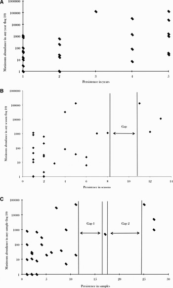
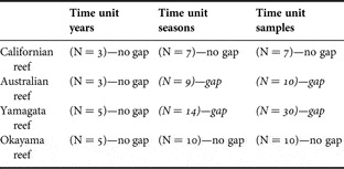
Table 1 summarizes the results obtained at the three different temporal scales. In case of the Californian and the Okayama reefs, this method failed in highlighting any gap. Concerning the Australian and the Yamagata reefs, it is worth underlying that without any time unit scale modification, it would have been impossible to distinguish any gap, as illustrated by Figure 2A. Nonetheless, discontinuities along the persistence axis became visible when increasing the number of time units by modifying the temporal scale (Figure 2B, C).
The plot of maximum abundance against persistence for the Yamagata reef at the three different time units: years (A), seasons (B) and samples (C). Note the log 10 scale on the Y-axis.

Plots results for each reef according to three different time units. Italic characters indicate the presence of a gap.

N, sample size.
For the Australian reef, whatever the time unit selected, the number of core species highlighted via this method equalled twelve and these species were similar in both cases. Concerning the Yamagata reef, three core species are underlined when using seasons as time units (the three species located on the right side of the gap are presented on Figure 2B). When using a sample time scale (Figure 2C), these three species are still shown as core species but it is then unclear if the core species group contains three or four species (i.e. whether the species located between the two gaps belongs to the resident or the transient group).
Fitting species occurrence patterns to a Poisson process
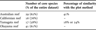
Conversely to the plot, this method can be applied to all four cases. According to the results obtained with this method, most of the species present in each dataset are classified as core. This is illustrated by Table 2. In all cases, core species represent more than 50% of the total number of species present in the dataset. This percentage even reaches 76% in the case of the Californian reef. All the species categorized as resident via the plot method (12 for the Australian reef and 3 or 4 for the Yamagata reef) are also perceived as resident according to this fitting method.
The number of core species highlighted by fitting a Poisson process to the species occurrence data.
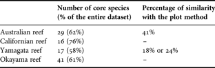
The percentage of similarity with the plot method indicates the degree of overlap between species categorized as core by the two methods. In case of the Yamagata reef, result varies according to the number of core species retained (3 or 4).
Reference to species' biological characteristics
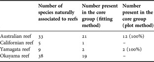
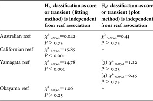
Regardless of the method employed and the dataset under scrutiny, when we look for overlap between methods, the majority of naturally-associated reef species are classified as transient species and not as core species (Table 3). Statistical analysis highlights this lack of relation between core species and naturally reef associated fish species (Table 4). As shown by the Chi-square test, results obtained by the plot and the Poisson fitting methods are in majority unrelated to fish biology. When significance appears (H0 rejected), contrary to what would be expected, it does not underline a link between core and reef-associated species but rather between transient and reef-associated species.
The relative importance of reef association in the classification as core species.

The number in parentheses in the right-hand side column indicates which percentage of the naturally reef-associated species, identified as core by the plot method, are also perceived as core by the fitting method.
Testing statistically the relation between the classification based on reef association and the classification based on the two other methods (plot and Poisson fitting).

The presence of two results for the Yamagata reef when dealing with the plot method depends on the number of core species selected (3 or 4).
Calculating the reciprocal form of the Simpson's index (D) for each persistence level species group and looking at its relation with regard to sample number
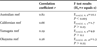
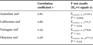
A shift in behaviour of D can only be detected when dealing with the Australian reef. Indeed, even at the whole dataset level (i.e. even when the most persistent groups have been included in the calculation and then when the rejection of H0 becomes the likeliest), H0 cannot be rejected for any of the three other case studies (Table 5).
Correlation coefficients and F test results for the four datasets once the most persistent species have been included in the calculation of D (i.e. when all the species are included in the calculation).
DISCUSSION
When plotting persistence against maximum abundance, a scale modification may be necessary to make gap appear, as illustrated by the Australian and the Yamagata reefs. Nonetheless, in case of the Yamagata reef, while a single gap appears when using seasons as temporal units, a double gap occurs when using sample number as time unit. This may constitute a potential problem, as it is not possible to determine, simply by looking at the plot, if the core species group includes or not the species located between the two gaps (Figure 2C). A solution may consist in checking whether the log normal model fits one of the two possible groups (3 species or 4 species), as core species abundance distribution is expected to follow a log normal distribution. A δ-corrected Kolmogorov–Smirnov test (Khamis, Reference Khamis1990) applied to the Yamagata reef dataset with samples as time units reveals that the log normal model fits better to the four-species group (D1,5 = 0.456; 0.5 > P > 0.2) than to the three-species group (D1,5 = 0.563: 0.2 > P > 0.1). However, this result is not, in itself, an ecologically-valuable proof (Magurran, Reference Magurran2005). Besides, we should note that however useful or necessary a time unit modification may appear, it also increases the risk of misclassification: a one year-long gap is much more ecologically significant than one season or a couple of samples. Therefore, we should be careful not to exaggerate the importance of the gaps highlighted by scale modification and systematically cross-check the result obtained with another method's output.
Conversely to the plot method, fitting the Poisson process to the species occurrence data provides classification for any dataset. Nonetheless, similarly to the plot method, problems are numerous. First, we would like to point out that if Magurran & Henderson (Reference Magurran and Henderson2003) propose this method as a starting point for sub-community analysis, they also notice that even with a 21-year-long dataset, it may lead to some misclassifications (three are reported). Therefore, as for the plot method, results should be crosschecked and this method should not be used exclusively. Second and even more important, the results generated do not appear as ecologically credible when compared with previous studies. Only a few studies based on objective distinction methods have been published so far and all but Magurran & Henderson (Reference Magurran and Henderson2003) referred to terrestrial communities (e.g. Hanski, Reference Hanski1982; Ulrich & Zalewski, Reference Ulrich and Zalewski2006). Whatever their focus, all these studies interestingly report a core species group smaller than the transient species group (i.e. less than 50% of the total number of species present in the assemblage). For instance, Magurran & Henderson highlight that 38.75% of the species sampled may be considered as core. As a result, the percentages displayed by Table 2 (from 58% of the species for the Yamagata reef to 76% for the Californian reef) appear as questionable, as they all present a majority of species as core. Finally, it is worth noting that while the Australian reef is associated with a similarity level almost twice as high as the Yamagata reef in Table 2, this is simply related to the relative increase of the core species group size: +242% for the Australian reef and +567% or +425% for the Yamagata reef, depending on the number of core species highlighted by the plot method (3 or 4). Indeed, for both reefs, the species categorized as core using the plot method are also present in the core species group according to this fitting method.
Adoption of the reef association characteristic as a distinction criterion would lead to produce misleading results involving persistence levels. For instance, if we consider the Yamagata reef (where 9 species are naturally present along reefs), Sebastes thompsoni (Jordan & Hubbs, 1925), a species present in 83% of the samples but not naturally associated with reefs, would be associated with the transient group. However, Pseudolabrus japonicas (Houttuyn, 1782), which is present in 10% of the samples or Girella punctata (Gray, 1835), which is recorded only once, would be categorized as core species with regard to their biological characteristics. A similar report may be done with regard to the Okayama reef: amongst the four species of cardinalfish (Apogonidae) which occur along the reef, two were present in 90% of the samples collected while the two others appeared only once. Beyond the question of the relative occurrence rate, the results obtained in this study clearly underline the weakness of the link, if any, between reef biological association and residence. This suggests that artificial reefs do not necessarily provide reef-specific habitats, but instead may provide suitable habitats for a wide range of fish species. Such a conclusion is consistent with Herrera et al. (Reference Herrera, Espino, Garrido and Haroun2002) and Walker et al. (Reference Walker, Henderson and Spieler2002) for instance.
Finally, looking for a shift in the relation between the reciprocal form of the Simpson's index and the number of samples collected failed to highlight a transition between log-series and log normal in the underlying distribution for most of our datasets. Two reasons may explain this failure: first, the two distributions may be impossible to distinguish due to the limited sample size of the datasets (Magurran, Reference Magurran2004). Indeed, the association core-log normal/transient-log-series may not be as clear as expected, preventing the reciprocal form of the Simpson index to mirror it. This possibility is clearly mentioned by Magurran & Henderson (Reference Magurran and Henderson2003): ‘As the time series lengthens we expect the modes of the two distributions to move apart and the division zone to become broader and clearer.’ Second, if core and transient species respectively follow a log normal and a log-series model in natural habitat communities, it remains unclear if similar patterns are generally observed when dealing with artificial habitat communities. For instance, Boisnier et al. (unpublished data, 2007) notice with reference to a dataset collected along a Japanese artificial reef during 7 consecutive years that the log normal distribution displays a better fit to both transient and core species. Besides, it is worth noting that even when this method succeeds in demonstrating a shift (Australian reef) the question of the boundary location between the two groups remains a challenge. As an illustration, if we remove the only species present in all the samples collected along the Australian reef, H0 cannot be rejected anymore (F0.05(2), 8, 8 = 1.73; P > 0.2; r = 0.27). In other words, the shift is statistically perceptible only when the single species present in all the collected samples is included. Should we then conclude that, according to this method, this species (i.e. Dinolestes lewini Griffith & Smith, 1834) is the only core species in the dataset collected along the Australian reef? We do not think so, as D behaviour simply mirrors a modification in the shape of the underlying distribution and should not be taken as an accurate indicator of the boundary between the two groups. This shift only occurs when the relative weight of the core species group (and their related log normal distribution) in the calculation becomes dominant. This dominance phase generally does not occur as soon as the first core species is integrated in the calculation process, but instead after a few transient species have already entered the calculation process, such that the shift cannot be considered as an indicator of boundary.
This study underlines clearly that none of these four objective distinction tools proposed by Magurran & Henderson (Reference Magurran and Henderson2003) appears as a suitable distinction method with reference to the four datasets selected, as several major problems were faced: first, tools may be unable to provide a result for each of the datasets considered. Second, the provided results may not be trustworthy from an ecological perspective. Third, results are extremely varied from one method to another, which means that it is not possible to use one method to cross-check the validity of another. Nonetheless, it should not be concluded that in any case, these four methods are unsuitable when dealing with artificial habitat community, as our datasets are not large enough for drawing such a general conclusion. We could then propose to collect samples similar to the one used by Magurran & Henderson (Reference Magurran and Henderson2003) but we believe that such a solution would simply be unrealistic. Indeed, similarly to the datasets selected in this study, the majority of the reef datasets reported in the literature ranges from a couple of months to a couple of years (e.g. Cummings, Reference Cummings1994; Tupper & Hunte, Reference Tupper and Hunte1998; Golani & Diamant, Reference Golani and Diamant1999; Moreno, Reference Moreno2002; Brotto et al., Reference Brotto, Krohling and Zalmon2007), depending on the study focus. From a general perspective, the use of relatively small datasets reflects the scientists' desire and the managers' need to be able to assess reef efficiency in a short period of time.
To conclude, Reed et al. (Reference Reed, Schroeter, Huang, Anderson and Ambrose2006) correctly emphasized that artificial reef assessment requires explicit standards. Despite its large presence in the artificial reef literature, the concept of fish residence cannot be currently considered as an explicit standard, as illustrated in this paper's introduction. Adopting a common, objective and accurate definition is required to reach such a status. Once fish residence becomes an explicit standard, the question of the optimum classification method becomes legitimate. However, trying to classify fish when categories' boundaries are not clearly identified makes little sense. Besides, the conclusions drawn by Magurran & Henderson (Reference Magurran and Henderson2003) suggest that, whatever the classification that may be used, the reliability of any classification will ultimately be related to sampling effort.
ACKNOWLEDGEMENTS
We thank Roshni Santiago, Nicola Cenacchi and the two anonymous referees for their valuable comments on successive drafts. Moreover, we are grateful to M. and T. Katayama from Ocean Construction Ltd (Okayama, Japan) for their constant cooperation. E. Boisnier's researches are financially supported by the JGC-Saneyoshi Scholarship Foundation (JGC Corporation, Japan).