NOMENCLATURE
- Re
-
Reynolds number
- RANS
-
Reynolds-Averaged Navier-Stokes
- CFD
-
Computational Fluid Dynamics
- HO
-
Higher-Order
- ILES
-
Implicit Large-Eddy Simulation
- SAE
-
Society of Automotive Engineers
- CFL
-
Courant-Friedrichs Lewy
- U 0
-
initial freestream velocity
- C p
-
coefficient of pressure
- C d
-
coefficient of drag
Greek Symbols
- Δ i
-
local i based length scale, where i takes cell, DES or RANS [m]
- δ
-
boundary-layer thickness [m]
- k
-
turbulence kinetic energy [m2/s2]
- ξ, η, ζ
-
curvilinear 3D grid coordinate system
- ν t
-
turbulent eddy viscosity [m2/s]
1.0 INTRODUCTION
As the use of Computational Fluid Dynamics (CFD) techniques become more widespread, the scale and the resolution of simulations used in aeronautical and automotive applications are consistently improving(Reference Sagaut and Deck1). Even with growing computational resources for majority of small-to-medium firms with access to multi-core workstations (~32 cores) or small computing clusters (<200 cores), turbulence-resolving methods for wall-bounded and high-Reynolds number flows remain a significant challenge, if not completely impractical. The original proposal of a Detached-Eddy Simulation (DES) initiated and inspired various hybrid turbulence modelling approaches, which seek to selectively treat regions of flow as either a Large-Eddy Simulation (LES) or a Reynolds-Averaged Navier-Stokes (RANS)(Reference Spalart, Deck, Shur and Squires2,Reference Islam, Decker, de Villiers, Jackson, Gines, Grahs, Gitt-Gehrke and Comas i Font3) . It is widely known that a RANS approach often provides insufficient accuracy and transient information for unsteady flows and at relatively high Reynolds numbers encountered in practice (~105–108) LES becomes prohibitive, especially in the presence of high-Re turbulent boundary layers(Reference Sagaut and Deck1,Reference Spalart, Deck, Shur and Squires2) . However, the complexity of some turbulence-resolving approaches, the implementation of accurate, unsteady boundary conditions and the need for high-quality grids designed specifically for DES have typically been seen as barriers to its wider industrial use. This work will seek to adapt DES for use with high-order numerical schemes in a CFD solver having steady boundary conditions on RANS-like grids, to assess the potential for its wider applicability.
Furthermore, it should be noted that based on the work by Chapman(Reference Chapman4) and Choi and Moin(Reference Choi and Moin5) fully resolved LES of wall-bounded flows are still well out of reach of most engineers and researchers interested in practical Reynolds number ranges of 105–108. With a freestream velocity corresponding to Re = 2 × 10⁵ for a flat plate turbulent boundary layer, the total number of points required in resolving the boundary layer is 30 with the first point at 0.95 × 10⁻⁵ m. The boundary-layer thickness is approximately 1.51 mm and these cells will only cover a tiny fraction of the entire computational domain, which is on the order of 103 m here and in typical automotive studies can be even larger(Reference Islam, Decker, de Villiers, Jackson, Gines, Grahs, Gitt-Gehrke and Comas i Font3,Reference Guilmineau, Deng and Wackers6–Reference Ashton and Revell8,Reference Islam and Thornber13) . Therefore, the total number of cells required for such a high-fidelity simulation can rapidly exceed 50 to 100 million cells.
This research employs a full-scale SAE 20° Notchback model at an industrially relevant Reynolds number defined as Re L = 2.3 × 10⁵. This geometry is standardised, and such reference models are often used to isolate typical flow features and understand fluid phenomena which are present on large, more detailed full-scale automotive models(Reference Islam, Decker, de Villiers, Jackson, Gines, Grahs, Gitt-Gehrke and Comas i Font3,Reference Le Good and Garry9) . The notchback with this particular slant angle better replicates impingement, A-pillar flow and three-dimensional structures and is a more appropriate test case, compared to simpler geometry such as an Ahmed body(Reference Wood, Passmore and Perry10). Experimental set-ups with such reference bodies are also simpler to replicate and computational expenses can also be reduced by eliminating and de-featuring unwanted, minor-scale details with negligible influence on the dominant flow features(Reference Le Good and Garry9).
Most common LES algorithms require a filtering operation on the governing equations(Reference Sagaut and Deck1) and explicitly model the influence of the unresolved scales of flow on the resolved features using a sub-grid model, which often rely on eddy-viscosity–based turbulence closures.
FLAMENCO(Reference Shanmuganathan, Youngs, Griffond, Thornber and Williams11–Reference Zhou and Thornber16) is the research CFD code used for this study and it relies on properties of non-oscillatory, non-linear numerical schemes(Reference Leveque17) to provide a low-dissipation framework which closely resembles the influence of conventional sub-grid scale explicit models(Reference Drikakis, Hahn, Mosedale and Thornber18–Reference Thornber, Drikakis, Williams and Youngs20). Hence, this computational solver is capable of Implicit Large-Eddy Simulation (ILES)(Reference Thornber and Drikakis21,Reference Thornber, Starr and Drikakis22) .
The implementation of DES with high-order numerical methods in a non-oscillatory, finite-volume framework is a novel approach. Although the use of first- or second-order numerical schemes is common in engineering, there are some instances where high-order methods are desirable. Separated flows can benefit greatly from high-order methods(Reference Islam and Thornber14). A high-order method is better able to resolve abrupt gradients and improve the resolution near discontinuities and in unsteady turbulent flows(Reference Garcia-Uceda Juarez, Raimo, Shapiro and Thornber12,Reference Leveque17) . Previous studies showed that the fifth-order method used here is equivalent to second-order results on eight times the number of grid points(Reference Shanmuganathan, Youngs, Griffond, Thornber and Williams11,Reference Drikakis, Hahn, Mosedale and Thornber18) and a reduction in the total grid sizes can drastically reduce computational expense and aid in wider adoption of hybrid turbulence-resolving methods.
Therefore, the primary objective of this work is to implement a modified DES algorithm in a fully compressible, all-Mach, finite-volume solver. Secondly, it will demonstrate the merits of this novel proposal in incorporating DES into a high-order accurate numerical framework. These methods are applied for an external aerodynamics simulation which is validated relative to averaged and time-dependent measurements, demonstrating that minimal user-interaction and case-specific calibration is required for practical, realistic flows. The first section includes a description of the computational domain and an outline of the numerical methods used. The Numerical Methods section contains information on the proposed hybrid turbulence model and the high-order schemes applied here. The use of experimental measurements is crucial in any correlation and validation study, so a brief description of the wind-tunnel setup is provided. The Results and Discussion section has been split into two distinct parts, the first containing results of validation against measured aerodynamic coefficients, a grid sensitivity study and a full Particle-Image Velocimetry comparison. This is followed a discussion of transient statistics from surface measurements and coherent turbulent structures around the bluff body.
2.0 COMPUTATIONAL APPROACH
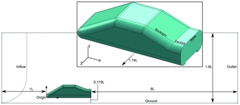
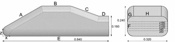
The overall dimensions of the notchback model were identical to the geometry tested inside the wind tunnel(Reference Wood, Passmore and Perry7,Reference Wood, Passmore and Perry10) and the details are provided in Figs 1 and 2. The main area of interest for this is the base surface at the rear of the notchback, and this required the extended 8 car lengths (L) downstream for the domain, with the total enclosure length being 10L to minimise the influence of the boundary conditions. The inlet for the CFD simulations was placed 1 car length upstream of the nose and although this is close to the stagnation region at the nose of the car based on past bluff body investigations(Reference Axelsson, Ramnefors and Gustafsson23), accurate inflow conditions were expected to minimise the impact on the results. High-resolution, turbulence-resolving simulations in existing literature, for example using an Ahmed body(Reference Guilmineau, Deng and Wackers6) also deemed 5L downstream distance to be sufficient. Preliminary studies conducted by the authors for a separate publication also revealed that increasing the overall domain size to 11L had minimal influence on the results(Reference Nader, Islam and Thornber24). The top and lateral boundary surfaces were enlarged compared to the wind-tunnel test section and were defined as free-shear walls.
Layout of the computational domain, major dimensions and the specified boundary conditions.

Envelope dimensions and C p inspection lines on the CFD coordinate axes. L = 0.840 mm.

The results were obtained with parallel CFD simulations running on a small-medium supercomputing facility. The distributed simulations ran over 4 nodes each having 24 compute cores, for a total of 96 cores. The medium grid resolution having 4.03 million cells required a total of 235 hours to reach the statistically steady state, equivalent to 11 non-dimensional cycles in the flow field. This computational cost can be drastically reduced through wall-modelling resulting in larger time-step sizes. In contrast, comparable studies with 16 million cell structured grids around an automotive bluff body took 337 hours and 600 hours on 384 compute cores, for URANS and DDES, respectively(Reference Ashton and Revell8).
2.1 Boundary conditions
Figure 1 highlights the main layout and the relevant separation distances of the major boundary conditions from the car model. The enclosure for the computational domain and the notchback model consisted of four boundary-condition types and their relative positions are defined. The side and top surfaces of the enclosure were defined as inviscid wall boundaries, since the experimental measurements were corrected for blockage effects(Reference Carr and Stapleford25) in the tunnel with boundary-layer growth on all outer surfaces. Additionally, a fully resolved boundary-layer mesh on all sides of the CFD enclosure would lead to a considerable increase in computational expenses, which would outweigh the minimal increases in accuracy for the flow phenomena considered here.
A Reynolds number of 2 × 10⁵ and a Mach number of 0.2 was used to calculate the relevant pressure and velocity at the inlet defined for the fully compressible solver. A steady inflow velocity was specified with a known boundary-layer thickness of 60 mm based on the wind-tunnel measurements and this was replicated using a Power Law as shown below
 $$\begin{equation}
\frac{u}{U_{0}}=\left(\frac{y}{\delta }\right)^{1/7}
\end{equation}$$
The outflow boundary employs a fixed pressure definition and extrapolates momentum and density terms to the boundary ghost cells. The car’s surfaces and the ground plane were both defined as viscous, no-slip wall boundariesm and these surfaces were used for all the integral force coefficients.
2.2 Notchback geometry
The original SAE reference notchback model included here featured rounded, filleted edges around the nose, the roofline and the backlight. The wind-tunnel measurements used as a validation test case in this investigation had a much larger research scope including the effects of yaw angle on the downstream flow behaviour. To reduce the yaw sensitivity within this Reynolds number range, the experimental programme recently modified the roofline to have a sharper interface with the fillets starting at the sides of the car model(Reference Wood, Passmore and Perry10). Therefore, this had a sharper edge around the roofline and backlight compared to Fig. 2. This also meant that the C p profiles on the decklid and slant at the furthest station from the centreline lay on the flat surface rather than on the rounded fillets and this was omitted from the comparative results discussed here. This was expected to have a minimal influence on the decklid or base surfaces at zero yaw configuration used for the CFD simulations presented here.
Although the bluff body is symmetric, the unsteady flow field and the resulting oscillations expected post-separation, especially at the rear led to the full flow-field being used for this series of simulations. This doubled the computational effort; however, it was an important inclusion in order to minimise the influence of an artificially imposed symmetry boundary condition on the separated shear layer and shedding vortices.
The wind-tunnel model was mounted on four 8-mm diameter slender posts and a shallow diffuser on the car’s underbody were removed from the domain to facilitate the creation of a high-quality structured mesh around the car. The influence of the diffuser was quantified previously in separate preliminary studies leading to a comparative article published on the notchback geometry(Reference Nader, Islam and Thornber24). Over the surface of the diffuser, the static pressure was 76% lower than the baseline configuration, and this led to some additional downforce as expected, although the pressure over the rest of the underbody remained nearly identical. The edges of the underbody diffuser also introduce small counter-rotating vortices into the wake and the upwash slightly alters the wake structure. The size of the recirculation and the vortex locations were translated by approximately 20 mm; however, such changes were locally contained and streamlines revealed that the overall flow features were similar.
LES boundary conditions need to include transient fluctuations to minimise the impractical amounts of flow time that would otherwise be required for the computational domain to achieve fully developed flow and sustain perturbations(Reference Rana, Thornber and Drikakis26). However, applied industrial simulations generally using RANS tend to have a fixed boundary condition based on a pressure, velocity or mass-flow value measured on the physical test setup. The velocity inflow here had a constant boundary-layer profile. Based on the wind-tunnel ground clearance, 20 mm of the total car model height was immersed within the boundary layer. This was replicated in the computational domain; however, there were no artificial inflow perturbations or turbulence intensity specified. Hence, the investigation is also expected to reveal whether fixed, steady boundary conditions practical for industrial applications could be used for high-fidelity simulations.
2.3 Grid generation
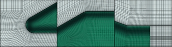
FLAMENCO is a structured, multi-block solver, and three different meshes were created with identical near-wall cell distances and first-cell y + value. Mesh details in the vicinity of the notchback model are provided in Fig. 3. In order to reduce computational expenses, the majority of the refinement was concentrated near the base and decklid surfaces, while avoiding abrupt transitions to the neighbouring blocks. The mesh was designed to be as close to Cartesian as practicable in the wake region to minimise numerical errors in the assessment of the curvilinear metrics.
Coarse 3D mesh details at the nose (left), roofline (middle) and the decklid (right).

An O-grid was generated around the whole vehicle, starting at nose of the car, and this was extended out downstream of the notchback model. This followed the rounded edges around the floor and the roofline, where the cells maintained the desired growth rate, radially outward and normal to the viscous wall surface of the car. The coarse mesh consisted of 3.25 million cells and successive refinement ratios varied within the range 1.2–2.3 for the entire domain. Table 1 presents detailed information about each of the grids used in this investigation.
Grid refinement levels with details of edge sizing corresponding to labels on Fig. 2

All the viscous wall surfaces were specified as y + = 1 and were fully resolved for this Reynolds number regime. It was challenging to achieve this resolution on the floor of the computational domain while maintaining the smooth O-grid around the bluff body mainly due to the relatively low ground clearance. A growth rate of 10% was defined around the notchback’s O-grid and this governed all the wall-normal spacing around it, before continuing as a C-grid down into the wake.
At some block interfaces further away from the notchback body, there are much higher growth rates. However, these were incidental side effects of tightly controlling the resolution within the C-O grid while also trying to minimise the total number of cells to reduce computational costs. It must be acknowledged that the finest mesh used in the study is quite coarse relative to some computational studies having 5 to 50 million cells around automotive bluff bodies(Reference Guilmineau, Deng and Wackers6,Reference Ashton and Revell8) . However, this illustrates the important contribution of the high-order numerical schemes to the overall accuracy, since past results(Reference Shanmuganathan, Youngs, Griffond, Thornber and Williams11) demonstrated that third- and fifth-order methods were comparable to doubling the resolution in each direction, leading to eight times the effective resolution. Furthermore, local velocity profiles extracted from the flow were used to demonstrate grid convergence in the Results and Discussion section.
3.0 NUMERICAL METHODS
3.1 Governing equations
The physics of fluid flow are modelled by the fully compressible Navier-Stokes equations in addition to the Stability-Enhanced Spalart-Allmaras turbulence model. The algorithm in FLAMENCO utilises a transformation to compute results in curvilinear coordinates (ξ, η, ζ) on multi-block, structured grids. The finite-volume, conservative form of the governing equations was used, facilitating further research with density variations due to thermal or acoustic perturbations in the future. In general curvilinear coordinates
 $$\begin{equation}
\frac{\partial {\mathbf {JU}}}{\partial {t}}+\frac{\partial {\mathbf {J\overline{F}}}}{\partial {\xi }}+\frac{\partial {\mathbf {J\overline{G}}}}{\partial {\eta }}+\frac{\partial {\mathbf {J\overline{H}}}}{\partial {\zeta }} = \frac{\partial {\mathbf {J\overline{F}_{v}}}}{\partial {\xi }}+\frac{\partial {\mathbf {J\overline{G}_{v}}}}{\partial {\eta }}+\frac{\partial {\mathbf {J\overline{H}_{v}}}}{\partial {\zeta }}+\mathbf {JS,}
\end{equation}$$
 $$\begin{equation}
\mathbf {J} = \frac{\partial {(x,y,z)}}{\partial {(\xi ,\eta ,\zeta )}},
\end{equation}$$
3.2 High-order numerical schemes
Very high-order numerical methods for partial differential equations arising from conservation laws have the following properties: achieve greater than second-order accuracy in smooth regions of flow, avoid spurious oscillations near shocks or high-gradients, and high-accuracy is achieved in shock-resolution(Reference Leveque17,Reference Toro, Spruce and Speares27) . The underlying numerical methods in FLAMENCO consist of augmented Godunov-type schemes(Reference Godunov28). Godunov’s method can essentially be defined as a three-step algorithm involving reconstruction, evolution and then averaging over cells for the conserved variable. Originally, Godunov’s method was limited to first-order accurate upwind schemes; however, non-linear schemes were used to provide greater numerical accuracy using high-order reconstruction and flux-limiters.
Results presented here used a Monotonic Upstream-Centered Scheme for Conservation Law (MUSCL) reconstruction scheme. Left and right edge states UL j ± 1/2 and UR j ± 1/2 are used to calculate a slope/profile within each cell, instead of the constant states in a first-order scheme. The fifth-order MUSCL formulation implemented in FLAMENCO was based on the approach by Kim and Kim(Reference Kim and Kim29). Reconstructed states from this can then be taken as an input to an approximate Riemann solver. The solutions here relied on a Harten-Lax-van Leer-Contact (HLLC) approximate solver which was originally introduced by Toro(Reference Toro, Spruce and Speares27,Reference Harten, Lax and van Leer30) . Therefore, the inviscid terms in the governing equations were resolved using fifth-order of accuracy and a second-order central scheme was used for the viscous and source terms. Low-Mach corrections were included in FLAMENCO to eliminate excessive dissipation characteristic of high-resolution Godunov-type schemes(Reference Thornber, Mosedale, Drikakis and Williams19,Reference Thornber, Drikakis, Williams and Youngs20,Reference Thornber and Drikakis31) .
Temporal discretisation used a second-order Strong Stability Preserving Runge-Kutta method (SSPRK)(Reference Spiteri and Ruuth32). This achieved additional stabilisation, which was needed for the high-order numerical schemes. The time-step size was chosen based on the Courant-Friedrichs-Lewy (CFL) condition. The SSPRK method imposed a CFL < 3 condition on time-step sizes; however, all the simulations presented here were time integrated using CFL = 0.8.
3.3 Turbulence modelling
Conventional DES employs a single turbulence model everywhere in the computational domain; however, it is treated as a sub-grid model in resolved regions and RANS mode near the walls. The DES algorithm implemented in FLAMENCO uses an Enhanced-Stability Spalart-Allmaras one-equation turbulence model. This is an eddy-viscosity model relying on the Boussinesq approximation for the closure of the turbulence terms, using a single equation for the variable
 $\widetilde{\nu }$
. A compressible form of the Spalart-Allmaras model is shown below.
 $$\begin{equation}
\frac{\partial \widetilde{\nu }}{\partial {t}}+\frac{\partial {(\widetilde{\nu }u_{j})}}{\partial {x_{i}}} = C_{b1}[1-f_{t2}]\widetilde{S}\widetilde{\nu }+\frac{1}{\sigma }\left\lbrace \nabla \cdot [(\nu +\widetilde{\nu })\nabla \widetilde{\nu }] + C_{b2}\left|\nabla {\nu }\right|^{2}\right\rbrace
\end{equation}$$
 $$\begin{eqnarray}
- \left[ C_{w1}f_{w}-\frac{C_{b1}}{\kappa ^{2}}f_{t2} \right]\left( \frac{\widetilde{\nu }}{\Delta } \right)+f_{t1}\Delta {U^{2}}, && \nonumber\\
\nu _{t} = \rho \widetilde{\nu }f_{\nu {1}} &&
\end{eqnarray}$$
Since FLAMENCO utilises a non-linear, high-order numerical framework there were several modifications introduced to the standard Spalart-Allmaras model to improve convergence encountered at laminar-turbulent interfaces and potentially, to eliminate negative eddy-viscosity values near boundary-cell curvature(Reference Burgess and Mavripalis33). This substitution turned off the production, destruction and the diffusion terms in the transport equation when in the affected region, and this led to an insensitive advection equation.
 $$\begin{equation}
\widetilde{\nu } = f_{\nu {1}}\Psi {\nu },
\end{equation}$$
 $$\begin{equation}
{\rm and}\ \Psi = \left\{\begin{array}{l@{\quad}l}
0.05{\rm log}(1-{\rm exp}(20\chi )), &\;\; x < 10 \\
\chi, & \;\; x \ge {10} \end{array}, \right.
\end{equation}$$
where f
ν1 is a model coefficient and
 $\chi =\widetilde{\nu }/\nu$
.
For the classical DES implemented in this high-order numerical framework, the performance of the RANS model was retained near the viscous-wall boundaries, on the tunnel floor and around the car model. The turbulence destruction term is affected by the new length-scale Δ which replaces the wall-distance d w , beyond the viscosity-affected regions of attached boundary layers. Hence, this is similar to classical DES; however, the outer length-scales are defined based on the local cell sizes calculated from the volume, rather than the maximum edge size (max(Δx, Δy, Δz)), which was found to be more robust to abrupt mesh changes and transitions found in practical, industrially relevant meshes. For the multi-block structured grid used here, the volume was obtained from the cell Jacobian (J).
 $$\begin{equation}
\Delta = {\rm min}(d_{w},\Delta _{cell}C_{DES})\ {\rm with}\ C_{DES}=0.65,
\end{equation}$$
 $$\begin{equation}
\Delta _{cell} = {3}\sqrt{\mathbf {J}}
\end{equation}$$
3.4 Turbulence length scales
Within the original RANS turbulence transport equation for
 $\widetilde{\nu },$
the wall-distance d
w
is used in the destruction term. This is modified for the DES implementation reported here, to a cell-based value; thus, the (
 $\widetilde{\nu }/\Delta$
) term is significantly higher in the outer regions of boundary layers and in the freestream. This is a significant modification because a global distance-based computation is being converted to use a local cell-based, scale estimate.
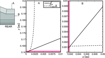
For the current geometry and domain configurations, the spatial variation in both the Δ length-scale (Equation (9)) and d
w
wall-distance were compared for the fine mesh in Fig. 4. Despite the use of grids which are coarse relative to majority of high-fidelity simulations performed on realistic geometries, it can be clearly observed that the local length-scales are up to a factor of 102 smaller than the wall-distance. Additionally, Fig. 4 also highlights the non-linear growth of the characteristic length-scale for the DES implementation relative to the original linear variation in wall-distance. This leads to a rapid increase in the eddy-viscosity destruction term and, when combined with the cell volume-based definition, becomes suitable for industrially relevant grids with abrupt transitions and skewness. The figure below demonstrates that the DES model switches away from RANS mode (Fig. 4 Red) and the destruction term of the
 $\widetilde{\nu }$
transport equation starts to decay at 1.3 mm above the decklid and 1.9 mm behind the base surface.
Variation in the wall distance d w and the DES length scale on the vertical (A) and horizontal (B) inspection lines at the rear of the vehicle. The red regions operated in RANS model.

4.0 EXPERIMENTAL MEASUREMENTS
4.1 Experimental set-up
The experimental measurements were taken inside Loughborough University’s 1.9 × 1.3 m wind tunnel. The inlet conditions were set to a maximum incident velocity of 40 m/s ± 0.4 m/s and a measured turbulence intensity of 0.2%(Reference Wood, Passmore and Perry10). The resulting flow field around the car was expected to be relatively Reynolds number insensitive. The in-draft wind tunnel has an open circuit and velocity profiles captured upstream of the test section revealed that it closely approximated a 1/7th power law, having a boundary-layer thickness of δ = 60 mm. Pressure coefficients were derived from measurements through the 110 pressure tappings distributed over the backlight, decklid and base surfaces. Freestream reference values were used and were corrected using MIRA blockage correction, derived based on continuity. This was also used for their pressure and the force coefficients measurements(Reference Carr and Stapleford25). This is defined as:
 $$\begin{equation}
C_{pCorr} = \frac{C_{pM}}{(1-A_{M}/A_{WT})^{-2},}
\end{equation}$$
where C pM is the model pressure coefficient, A M is the model frontal area and A WT is the wind-tunnel cross-section area. This leads to a coefficient value which is more representative of that expected under freestream conditions. Time-statistics were deduced from 31 seconds of sampled data at 260 Hz and the scanners had an accuracy of ±1.47 Pa. PIV measurements were time-averaged from 1,000 instantaneous vector fields and there was a 50% overlap ratio for the 32 × 32 effective inspection window. The experimental measurements were sampled for 30 seconds to obtain the mean values for lift C l and drag C d coefficients. The reported accuracy(Reference Wood, Passmore and Perry10) of the underfloor balances were ±2 drag counts or 0.002 for a 1/4 scale model.
4.2 Expected flow features
Based on the past studies conducted by Gaylard, Howell and Gary(Reference Gaylard, Howell and Garry34) and Wood, Passmore and Perry(Reference Wood, Passmore and Perry10) on similar bluff bodies, there were a few common flow features expected in this investigation in wake of a notchback model. The relatively close proximity to the ground, h/L = 0.119, was expected to accelerate the flow underneath the vehicle, and an upwash was expected immediately post-separation at the rearmost edge of the car. This is expected to interact with and distort the low-pressure wake, as observed from Particle Image Velocimetry (PIV) measurements. Subtle separation was expected from the 20° notchback model at this Reynolds number based on similar full-car models in past studies; however, this was not captured in the wind-tunnel measurements. The predictive capability of the high-resolution CFD is utilised to gain a better understanding of the flow, especially in areas where measurements were impossible or limited by physical proximity to experimental equipment.
Over the backlight and the decklid, the shear-layer separation and impingement are expected to be challenging flow features to predict using CFD, primarily due to the adverse pressure gradient, grid resolution limitations and localised laminar-turbulent transitions. Gaylard et al(Reference Gaylard, Howell and Garry34) also revealed that there is a periodic variation of the unsteady features in the lateral direction to the car and this was monitored with the instantaneous CFD results. Hairpin vortices over the backlight and decklid are also expected, and this is likely to pose a challenge to attempts at capturing accurate surface pressure profiles and vortex locations. Immediately downstream of the base surface the flow field is expected to contain primary and secondary recirculation regions. Combined with the shear-layer separation over the backlight, they are expected to oscillate at various frequencies and can be identified from frequency domain data.
5.0 RESULTS AND DISCUSSIONS
It is important to note that to the best of our knowledge, this is the first comprehensive aerodynamic study of the SAE Notchback model and given the diverse flow features which are generated around this geometry combining both sharp-edged and subtle pressure-induced separation, this series of studies(Reference Islam and Thornber13,Reference Nader, Islam and Thornber24) seeks to add significant value to the research community. Results from the frequency domain analysis used a total of 1.02 million data points representing individual time-steps. The results presented here mainly focus on the rear of the car model due to its significance in overall drag and as the most challenging region for RANS simulations. The experimental error bounds were calculated from the tolerance of the pressure transducers and the uncertainty in freestream conditions.
5.1 Validation of computational results
5.1.1 Mean aerodynamic coefficients
The notchback model in the zero-yaw configuration exhibited a mean drag coefficient C d = 0.207 and C l = 0.0548. The high-order CFD results generated a mean C d = 0.237 and C l = 0.0628, which represents an over-prediction of 14.5% and the lift coefficient was over-predicted by 21.7%.
There were two important changes that have an impact on the mean force coefficients, the underbody diffuser and smooth longitudinal edges of the notchback. The longitudinal edges were originally smooth for the notchback model provided through the Loughborough Repository, which differed from the the figures presented by Wood et al(Reference Wood, Passmore and Perry10); however, this was altered in a later revision to the Loughborough Repository(Reference Wood, Passmore and Perry7). The information on the sharp-edge model was only made available after the simulations were completed, and it was not practical to change them at the time of writing. Given that the intent of the edge modification was to reduce the Reynolds sensitivity at yaw angles that were used in the experimental study, it was not expected to alter the main coherent structures in the baseline configuration aligned with the freestream. We acknowledge that that backlight surface will be the most dramatically affected, possibly with stronger vortices along the outboard edges.
The influence of the diffuser was quantified previously in separate studies on the Notchback geometry(Reference Nader, Islam and Thornber24). The RANS results from that investigation predicted C d = 0.097 with the diffuser and C d = 0.121 as baseline, representing 53% and 41.5% errors, respectively. Over the surface of the diffuser, the local static pressure was 76% lower than the baseline configuration, and this led to some additional downforce and underbody diffuser edges also introduce small counter-rotating vortices into the wake, slightly altering the upwash. As a result, the main lower vortex was translated closer to the bluff body by approximately 20 mm; however, such changes were locally contained and streamlines revealed that the overall flow features were comparable. Given only 7.5 million cells were used, the high-order DES approach better than RANS with up to 16 million cells. Hence, current results were an improvement over RANS approaches, even without the diffuser geometry reducing the total drag, which was over-predicted relative to experiments.
5.1.2 Wake and base surface sensitivity
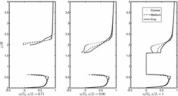
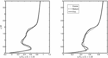
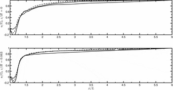
To illustrate grid independence and have greater confidence in the reported results, local flow quantities around the bluff body generated by all three resolution levels were compared. These included 5 vertical and 2 horizontal line samples that were time-averaged for 11 non-dimensional cycles over the length of the body (L = 0.840 m).
The first three sampling locations (Fig. 5) were on the middle of the backlight, the start of the decklid surface and at the trailing edge, respectively. The subtle separation bubble over the backlight is greatly influenced by the resolution of the smooth, curved edge at the intersection with the roof surface. This led to the coarser grids slightly over-predicting the recirculation region and the finest velocity profile appears to be closer to an attached boundary layer. A similar difference was observed in the underbody, as this was not adequately resolved by the coarser grids. However, the maximum differences in the entire profile was <11.5%. This area was particularly sensitive due to the cell sizes being crucial in defining the surface curvature accurately.
Normalised streamwise velocity profiles at 3 stations on the central longitudinal plane.

Normalised streamwise velocity profiles at 2 dowstream stations on the central longitudinal plane.

At the start of the decklid, the recovered flow profile impinges upon the surface and this is another challenging region to capture with limited grid resolution. The medium and fine meshes both captured the recirculation in the u/U 0 profile with a difference of 9.2%. Although the magnitude of the underbody velocity profile was nearly identical, the location of the peak was closer to the floor of the bluff body for the coarser grids. At the notchback trailing edge, the improvements in the mean velocity profiles decreased with successive mesh refinement, as highlighted by the third profile in Fig. 5. The transition from medium to fine mesh led to local velocity changes that were approximately half of that observed in the coarse-medium mesh refinement.
The last two vertical line sampling locations were in the near wake of the notchback. All three profiles follow a similar trend however, the medium and fine mesh better captured the peak velocity from the upwash at both x = 1.31L and 1.43L locations. There was a maximum of 4.2% error between the finer profiles and the coarsest grid predicted a vortex location closer to the ground.
Figures 5 –7 highlight the impact of mesh refinement. The base surface of the notchback is the most challenging region in the flow field due to the high turbulence intensity and the fluctuating low-pressure wake.
Normalised streamwise velocity profiles at 2 horizontal downstream stations at 0.05 m above ground.

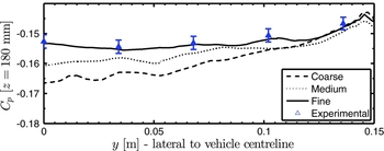
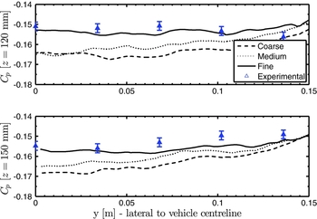
The predicted C p showed consistent improvement over the entire range of y values. At the top profile (Fig. 8) the time-averaged data reveals that the errors closer to the vehicle centreline were larger and this region was the most challenging for the coarser mesh resolutions. The fine mesh however was able to achieve capture pressure coefficients with <2.15% error over entire range. This is well within the range of experimental uncertainty.
Pressure coefficient profiles on the base surface 140 mm above the car underbody.

Moving closer to the middle of the base surface, the profiles at z = 120 and 150 mm elevation (Fig. 9) a similar trend is observed with the mesh refinement. The fine mesh results at z = 120 mm matched the experimental C p data for all points except at y = 136 mm from the centreline, where the lower pressure might indicate presence of a secondary vortex due to the swept fluid from the side surface of the car. The upwash around the side of the vehicle was also captured in Fig. 13. A maximum error of 2.45% was obtained by the fine mesh, relative to experimental measurements and all the CFD profiles successfully followed the trend with the inboard locations furthest from the measured data, consistent with previous observations. The z = 150 mm profile was even more accurately captured, with average and peak errors of 0.46% and 1.67%, respectively.
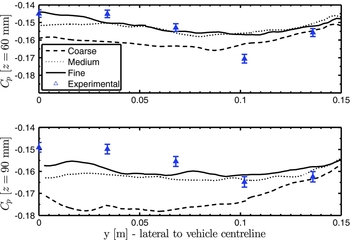
Pressure coefficient profiles on the base surface at 110 mm (bottom) and 80 mm (top) above the car underbody.

At the two lowest inspection stations, the experimental C p profiles had greater standard deviation, with low-pressure vortex cores identified near y = 100 m (Fig. 10). The medium and fine meshes had very similar results and led to 8.03% maximal errors however, the strong vortex at y = 102 mm position was not captured adequately by any of the simulations. There was a 5.64% maximum error in the fine mesh results compared to the tunnel measurements and the central, inboard region was the most challenging to capture using CFD, especially due to the mounting struts and the underbody diffuser which were de-featured.
Pressure coefficient profiles at 50 mm (bottom) and 20 mm (top) above the car underbody.

The figures presented here experimentally validates the simulation results and based on the velocity profiles at 7 different locations and 5 different profiles on the base surface, the fine mesh was deemed sufficient for this study. Although the accuracy of some mean and unsteady flow quantities could be improved even further, the time-step limitations would lead to a large increase in computational costs. The finest mesh resolution used here lies at the lower end of the spectrum compared to many existing turbulence-resolving bluff body simulations(Reference Guilmineau, Deng and Wackers6,Reference Ashton and Revell8) and it is evident that the central part of the base surface is the most resource intensive. However, this challenging setup illustrates the capability of the modified DES in a high-order accurate numerical framework.
5.2 Particle-image velocimetry (PIV) comparison
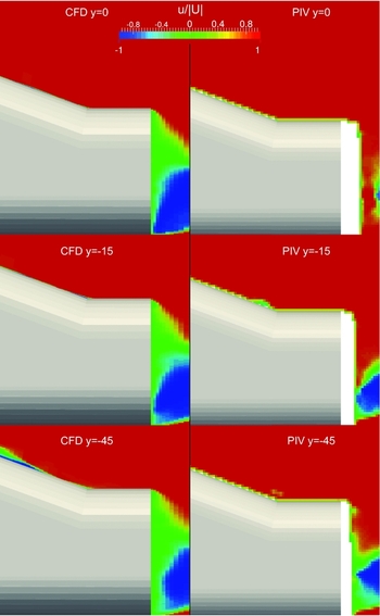
The size and the location of the primary recirculation region and the shear-layer detachment from the decklid were more uniform in the CFD results, as shown on the planes moving outboard towards y = −45 mm. The PIV results captured higher velocities near the decklid compared to CFD however, conclusions on accuracy and predictive capability cannot be drawn from this since the measaurements had limited resolution in this region and CFD better visualised the interaction of the detached shear-layer and recirculation in the wake.
Additionally, CFD results revealed a small region of lower velocity, similar to a subtle separation bubble midway along the backlight at the y = −45 mm plane. This is related to the hairpin vortices which were observed along the central plane of the model, arising from the roofline and continuing downstream, visualised using iso-surfaces (Fig. 13). It should be noted that based on the velocity profile comparison during the grid refinement study, the size of this separation bubble was decreasing with increased resolution, so it may be closely related to upstream disturbances introduction by the roof trailing edge curvature, thereby also making it more grid-sensitive.
The primary recirculation region in the PIV results was further away from the base surface and the CFD results seem revealed a much larger influence of the trailing, side vortices directed upwards along the side surface of the car. Overall, the CFD results were able to accurately locate the minima of normalised velocity in the wake and the influence of the upwash from the ground reference plane, as it deformed the recirculation region in blue (Fig. 11).
Particle Image Velocimetry (PIV) comparison on longitudinal planes at the rear. Blanked areas on the PIV dataset represent areas that could not be captured.

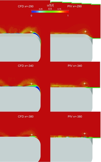
Inspection planes normal to the car’s longitudinal centreline (Fig. 12) reveal the presence of vortical flow structures. Generally, the vortices over the backlight were stronger in CFD, identified using a combination of low-pressure cores and vorticity. At the x = −290 mm plane, lying at the intersection of the backlight and decklid, the vortex locations and centreline velocity deficit was accurately captured (Table 2). At the x = −340 mm plane lying on the decklid, the vortex size is larger in the CFD results and translated inboard compared to PIV. The lower velocity further inboard, likely resulted from stronger impingement and deceleration of the flow, and the smoother outer edges in the CFD geometry translating vortices inboard at the last two planes.
Particle Image Velocimetry (PIV) comparison on the cross-stream planes at the rear. Blanked areas on the PIV dataset represent areas that could not be captured.

Vortex core location comparison based on cross-stream PIV planes and CFD results from Fig. 12. Note that the PIV measurements were based on the wind-tunnel coordinate system - Y (lateral), Z (vertical)

5.3 Vortices and coherent structures
Due to the three-dimensional nature of the flow features downstream of the car model, it is often appropriate to use specific flow variables such as strain rates or vorticity to understand fluid behaviour. The present work employed the Q-criterion defined below to capture and visualise coherent structures which develop over time(Reference Hunt, Wray and Moin35)
 $$\begin{equation}
Q=\frac{1}{2}(\Omega _{ij}^{2}-S_{ij}^{2})>0
\end{equation}$$
This isolates the regions of flow where the vorticity tensor dominates the strain-rate tensor and this was used to generate the iso-surfaces reported here (Fig. 13).
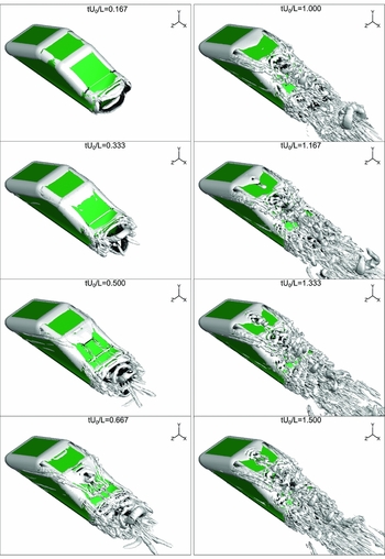
Development of the unsteady, coherent flow structures visualised using the Q-criterion, Q = 800 [1/s].

Q-criterion iso-surfaces (Fig. 13) indicated presence of vortex sheets oriented vertically and horizontally, from the trailing edges of the notchback. There was a large horseshoe vortex around the nose, which enhanced the longitudinal vortices diagonally upwards around the side of the car. The separated flow over the roof and the central plane along the backlight was well predicted by CFD. This shear-layer separation was energising the flow over the backlight and the separation bubble size was sensitive to local resolution. These coherent structures (Fig. 13), such as the prominent trailing vortices for tU 0/L > 0.67 interact with the subtle separation bubble over the backlight as shown in CFD results. These also impinge on the decklid surface.
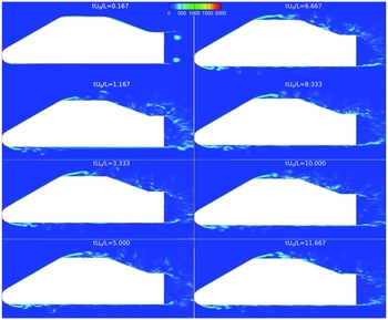
The central plane through the car model revealed thin regions of fluid rising after subtle separation on the roof and backlight, which was captured by both the iso-surfaces (Fig. 13) and the contours coloured by vorticity (Fig. 14). The shear-layer separation and the oscillations in the flow were sustained well after a statistically steady flow period was reached, as revealed by the instances tU 0/L > 6.
Two-dimensional filled contours coloured with vorticity Ω [1/s].

These iso-surfaces also show the start-up process and growth of the roll-up vortices downstream (Fig. 13). The period captured in the figures emphasis the transient start-up in the first 1.5−1.6 non-dimensional cycles, to illustrate the source and growth of the major coherent structures.
5.4 RMS transient statistics
One of the major advantages of high-fidelity, unsteady simulations is the ability to capture time-dependent flow features which are damped in conventional RANS approaches. Even using Unsteady-RANS (URANS), turbulence time-scales in highly-separated flow which are smaller than the effective averaging period are missed. For the entire flow field the standard deviation about the mean values were computed for all variables, as shown below
 $$\begin{equation}
RMS_{i} = \sqrt{\overline{(\phi _{i}-\overline{\phi }_{i})^{2}}}
\end{equation}$$
where the ϕ i represents an arbitrary flow variable and the bar represents a time-averaging operation. In this case, it reveals the intensity of the fluctuations in the flow field.
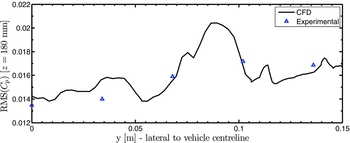
Referring back to the base inspection locations (Fig. 1), the top profile at z = 180 (Fig. 15) for RMS of C p follows the experimental measurements quite closely and matches the trend with the increasing gradient towards the outboard direction. Note that the wind-tunnel coordinate origin (global z) was placed on the inspection section floor and hence, a clearance of 40 mm was present and these are offset in the graphs presented here. The CFD results predicted some very large fluctuations, between each of the inspection points on the car model and given the lack of resolution in the experimental measurements, it is difficult to comment on the accuracy of the profiles in these regions. The largest error of 8.3% was observed at the y = 34 mm location. Time-convergence studies with additional flow cycles revealed negligible differences in the CFD results and hence, the high fluctuations are believed to be physically valid.
RMS of C p at 140 mm above the car underbody.

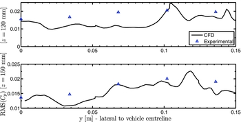
RMS of C p at 80 mm (top) and 110 mm (bottom) above car underbody.

The pressure RMS values at the top elevation was the lowest as expected. The profiles at z = 120 and z = 150 mm elevation (Fig. 16) exhibited features which were the most challenging to replicate using CFD and this agrees with the trend observed in the mean C p results with the central area of the base surface being grid-sensitive. The location of the maximal error moves further outboard to y = 68 mm from the centreline. The overall trend was still captured well however, this 38% error is an isolated reading, likely due to trailing vortices considering the significantly improved average error of 7.2% over the remainder of the inspection points. The average and maximum RMS errors relative to experimental data fell to 10.3% and 18%, respectively at the z = 150 mm elevation.
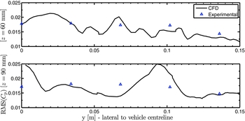
RMS of C p at 20 mm (top) and 50 mm (bottom) above car underbody.

At the z = 90 mm elevation (Fig. 17) there was another region of high fluctuation predicted by the CFD for 75 < y < 100 mm and the errors around this region were 16% and 11%. Flow around the centreline led to the largest errors and the average error of 5.9% was achieved relative to the wind-tunnel measurements. The simulated results performed the best on the lowest profile at z = 60 mm, which is 20 mm above the car’s underbody. An average error of 2.3% was recorded along this profile. Although experimental measurements captured a higher velocity magnitude compared to the CFD at the second-most outboard location, this is likely due to the diffuser edge and mounting pins which were defeatured in CFD. Additionally, the RMS values obtained from CFD were accurate over the entire profile.
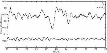
The integral forces of lift and drag and the oscillations in the dataset were used to further investigate the unsteady flow phenomena (Fig. 18). The unsteady drag coefficient had a higher standard deviation of 0.0363 compared to 0.0061 for the lift and this agrees with the greater variation in the signal amplitude. The lift coefficient was more periodic with a smaller range of active frequencies. This was expected due to the total drag of the car being primarily governed by the large low-pressure wake, while the instantaneous lift profile was governed by the smaller shedding vortices.
Unsteady force coefficients showing 10 cycles of the extended simulation (t f = 28L/U 0).

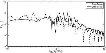
With this particular combination of freestream variables and the characteristic length of the car, the cycle time (L/U 0) is approximately 0.3 seconds. Based on the Fast Fourier-Transform (FFT) performed on the time-dependent data (Fig. 18) several dominant modes of oscillation were obtained. The power spectrum was plotted against frequency content on logarithmic axes (Fig. 19) and the lift-coefficient data predicted higher dominant frequencies than the drag-coefficient. Most significant peaks were identified at 2.43, 3.35 and 6.08 Hz, which corresponded well with the expected 0.35 second period of flow evolving over the entire car (L/U 0) and dominant Strouhal number of 1.19.
Spectral analysis of the integral forces recorded for the notchback body.

One of the most interesting features was evident on the drag coefficient (Fig. 18) profile with a regular, periodic jump in the drag amplitude seen near t = 18L/U 0 and t = 22.5L/U 0. This directly corresponds to the 6 Hz peak frequency observed in the spectrum. This resulted from the periodic migration of the low pressure wake forwards and backwards along the longitudinal axis, causing a regular variation in the base surface pressure, thereby affecting total drag. Secondary coherent features were also identified, so the higher 14–17 Hz frequencies likely resulted from smaller scales in the separated shear layers.
6.0 CONCLUSIONS
This full-scale study of an SAE notchback model adopted a DES approach with high-order accurate numerical schemes to simulate external aerodynamics, validate against wind-tunnel measurements and to predict unsteady flow features. The DES algorithm implemented with an Enhanced-Stability Spalart-Allmaras model was a novel approach, especially at the Reynolds number regime considered here. Despite the lack of transient, turbulent content or artificial sources of perturbations commonly used with LES or DES studies, this novel DES implementation proved successful on the multiblock meshes generated for the notchback model and successive mesh refinement revealed smaller coherent structures and C p profiles were captured more accurately. The most significant errors could be attributed to the removal of the mounting struts, the diffuser and also the inclusion of rounded fillets on the longitudinal edges. Despite the de-featured underbody and given only 7.5 million cells were used, the high-order DES algorithm performed significantly better compared to RANS with up to 16 million cells. Results had better agreement with experimental measurements for C d and C l , with maximum improvement of 38% on time-averaged quantities.
Iso-surfaces of Q-criterion revealed that the coherent flow structures reach a steady-state after 1.5 non-dimensional periods (tU 0/L) from the initial start-up. DES functionality was demonstrated and by inspecting the local turbulence length scales it was found that the Δ definition was an order of 102 smaller than wall-distances around the car’s surfaces. Both streamwise and cross-stream normalised velocities were compared to PIV data and it was observed that the CFD results were more uniform in the lateral direction while the inboard locations revealed smaller recirculation regions. The largest difference was observed just post-separation in the shear layer. Vortex core positions were compared and a maximum positional error of 6.7% was obtained in the intersection between the backlight and decklid. This is a region which could benefit from greater mesh resolution and the higher lateral velocity in the CFD results moved the vortices further inboard.
RMS and time-averaged C p profiles exhibited consistent improvements with mesh refinement and fine results were within 6% of experimental data. Spectral analysis identified primary and secondary modes of vortex shedding with frequency range of 2–6 Hz. Future studies on this model will include larger grids consisting of 10–40 million cells, as representative of the state-of-the-art in hybrid modelling. Currently, in addition to the earlier work by the authors, this is the only known comprehensive series of CFD simulations for the SAE Notchback model so it seeks to add significant value to the research community.
ACKNOWLEDGEMENTS
The authors would like to acknowledge Intersect HPC Orange (NCMAS 2015 grant EX5) and the University of Sydney HPC service (Artemis) for providing HPC resources that have contributed to the results reported here. The experimental measurements shared by Loughborough University Automotive and Aeronautical Engineering Department greatly assisted this investigation and led to this geometry being used as a benchmark for current and future studies. We would also like to thank Adrian Gaylard at Jaguar Land Rover UK for our valuable discussions on bluff body aerodynamics.