1 Introduction
Most superhydrophobic surfaces (SHSs) are textured (i.e. made of ridges or posts), and they can entrap air within the cavities when they are submerged in water. Due to the slip at the interface between water and air, the skin-friction drag on SHSs can be less than that on a flat and smooth surface (Rothstein Reference Rothstein2010). The amount of drag reduction (DR) on an SHS in laminar flow is theoretically predictable (Lauga & Stone Reference Lauga and Stone2003; Belyaev & Vinogradova Reference Belyaev and Vinogradova2010; Busse et al. Reference Busse, Sandham, McHale and Newton2013), but that in turbulent flow is unpredictable, and thus experimental studies have been conducted to investigate DR in turbulent flows (Watanabe, Yanuar & Udagawa Reference Watanabe and Udagawa1999; Zhao, Du & Shi Reference Zhao, Du and Shi2007; Daniello, Waterhouse & Rothstein Reference Daniello, Waterhouse and Rothstein2009; Peguero & Breuer Reference Peguero, Breuer and Eckhardt2009; Woolford et al. Reference Woolford, Prince, Maynes and Webb2009; Jung & Bhushan Reference Jung and Bhushan2010; Aljallis et al. Reference Aljallis, Sarshar, Datla, Sikka, Jones and Choi2013; Park, Sun & Kim Reference Park, Sun and Kim2014). While Daniello et al. (Reference Daniello, Waterhouse and Rothstein2009) and Park et al. (Reference Park, Sun and Kim2014) experimentally showed significant turbulent DRs (50 % and 75 % respectively) with SHSs, others reported negligible DR or even drag increase in a turbulent flow (Watanabe et al. Reference Watanabe and Udagawa1999; Zhao et al. Reference Zhao, Du and Shi2007; Peguero & Breuer Reference Peguero, Breuer and Eckhardt2009; Aljallis et al. Reference Aljallis, Sarshar, Datla, Sikka, Jones and Choi2013). This inconsistency may be explained by the air loss inside cavities (known as the Wenzel state), deformation of an air–water interface, errors in measuring friction drag, etc. (Park et al. Reference Park, Sun and Kim2014).
To understand the flow changes and mechanism of DR by SHSs, many numerical studies have been conducted (Min & Kim Reference Min and Kim2004; Fukagata, Kasagi & Koumoutsakos Reference Fukagata, Kasagi and Koumoutsakos2006; Martell, Perot & Rothstein Reference Martell, Perot and Rothstein2009; Busse & Sandham Reference Busse and Sandham2012; Park, Park & Kim Reference Park, Park and Kim2013; Jelly, Jung & Zaki Reference Jelly, Jung and Zaki2014; Türk et al.
Reference Türk, Daschiel, Stroh, Hasegawa and Frohnapfel2014; Rastegari & Akhavan Reference Rastegari and Akhavan2015; Seo, García-Mayoral & Mani Reference Seo, García-Mayoral and Mani2015). In these studies, due to the difficulties of numerically handling the dynamics of the interface between water and air, either a slip length (to be defined later) or a shear-free condition has been provided as a boundary condition at the interface without solving the air layer. These numerical studies have reported DR in turbulent flow, and provided the mechanism by which DR was achieved. Min & Kim (Reference Min and Kim2004) showed that the turbulent drag is reduced by streamwise slip but increased by spanwise slip. Fukagata et al. (Reference Fukagata, Kasagi and Koumoutsakos2006) proposed an empirical formula for the DR rate. Busse & Sandham (Reference Busse and Sandham2012) investigated the effects of the anisotropic slip by providing prescribed slip lengths in wall-parallel directions. Martell et al. (Reference Martell, Perot and Rothstein2009) simulated the flows over longitudinal grooves and square posts by using mixed boundary conditions consisting of no-slip (solid–water interface) and no-shear (air–water interface) regions. Park et al. (Reference Park, Park and Kim2013) found, by considering different SHS geometries and Reynolds numbers, that the amount of turbulent DR is well correlated with the slip length normalized by the viscous wall unit. Jelly et al. (Reference Jelly, Jung and Zaki2014) addressed the effect of secondary flow induced by the edges of the longitudinal groove, and Türk et al. (Reference Türk, Daschiel, Stroh, Hasegawa and Frohnapfel2014) found that the groove width significantly changes the flow pattern. More recently, Rastegari & Akhavan (Reference Rastegari and Akhavan2015) suggested that the amount of DR should be expressed as the sum of the slip velocity and the modifications of the Reynolds shear stress and mean convective stress. Seo et al. (Reference Seo, García-Mayoral and Mani2015) investigated the effect of the surface geometry (i.e. longitudinal grooves versus square posts) on pressure fluctuations at the interface and suggested a relationship between the slip velocity and the root-mean-square (r.m.s.) pressure fluctuations at the interface. In particular, Türk et al. (Reference Türk, Daschiel, Stroh, Hasegawa and Frohnapfel2014) and Seo et al. (Reference Seo, García-Mayoral and Mani2015) examined the sustainability of the interface between water and air against turbulent pressure fluctuations. They showed that the maintenance of the air–water interface depends on the pattern sizes of SHSs, and reported that the maximum sizes of the longitudinal grooves and square posts for its maintenance are approximately 150 and 50 wall units respectively. Seo et al. (Reference Seo, García-Mayoral and Mani2015) also showed that the interface deformation by turbulent pressure fluctuations is negligible when the pattern size of an SHS is equal to 6 wall units, with a capillary number of
 $Ca=6\times 10^{-3}$
, where
 $Ca={\it\mu}_{l}u_{{\it\tau}}/{\it\sigma}$
,
 ${\it\mu}_{l}$
is the water viscosity,
 $u_{{\it\tau}}$
is the shear velocity and
 ${\it\sigma}$
is the surface tension between air and water (
 ${\it\sigma}=0.073~\text{N m}^{-1}$
). Piao & Park (Reference Piao and Park2015) modelled pressure fluctuations at the interface as a harmonic oscillation and suggested that the pattern size of an SHS should be
 $O({\rm\mu}\text{m})$
for the air–water interface to be stable.
Despite many achievements through previous numerical studies on turbulent flows, none of them have considered the air layer over SHSs but all of them have modelled it by prescribing either a slip length (Min & Kim Reference Min and Kim2004; Fukagata et al. Reference Fukagata, Kasagi and Koumoutsakos2006; Busse & Sandham Reference Busse and Sandham2012) or a shear-free condition (Martell et al. Reference Martell, Perot and Rothstein2009; Park et al. Reference Park, Park and Kim2013; Jelly et al. Reference Jelly, Jung and Zaki2014; Türk et al. Reference Türk, Daschiel, Stroh, Hasegawa and Frohnapfel2014; Rastegari & Akhavan Reference Rastegari and Akhavan2015; Seo et al. Reference Seo, García-Mayoral and Mani2015) at the interface. Only a few studies have considered the air layer for laminar flow assuming a flat air–water interface (Tretheway & Meinhart Reference Tretheway and Meinhart2004; Davies et al. Reference Davies, Maynes, Webb and Woolford2006; Maynes et al. Reference Maynes, Jeffs, Woolford and Webb2007; Busse et al. Reference Busse, Sandham, McHale and Newton2013). Therefore, in the present study, we perform direct numerical simulations (DNS) of a turbulent channel flow with an air layer over an SHS. We also assume that the air–water interface is flat and thus the surface tension is neglected. With this problem setting, we can identify the effect of the air layer on the slip behaviour at the interface and the skin-friction reduction. We consider two different flow types inside the air layer: in case 1, the flow inside the air layer is shear-driven at the top of the air layer (Joseph Reference Joseph1980; Vinogradova Reference Vinogradova1999); in case 2, the flow recirculates inside the air layer and thus its net mass flow rate is zero (Maynes et al. Reference Maynes, Jeffs, Woolford and Webb2007; Busse et al. Reference Busse, Sandham, McHale and Newton2013). The air layer in case 1 is an approximate model for longitudinal (streamwise) grooves, whereas in case 2 the air contained in the air layer is trapped (practical explanations of this case were described in Busse et al. (Reference Busse, Sandham, McHale and Newton2013)). In both cases, the analytical solutions of laminar flow can be readily obtained (Joseph Reference Joseph1980; Busse et al. Reference Busse, Sandham, McHale and Newton2013).
The present results are compared with those from previous studies using the Navier slip model without solving the air layer that provides slip velocities in the streamwise and spanwise directions at the air–water interface as
 $u_{s}=b_{x}(\partial u/\partial y)_{s}$
and
 $w_{s}=b_{z}(\partial w/\partial y)_{s}$
, where
 $b_{x}$
and
 $b_{z}$
are the streamwise and spanwise slip lengths, and
 $(\partial u/\partial y)_{s}$
and
 $(\partial w/\partial y)_{s}$
are the streamwise and spanwise shear rates at the interface respectively (Hahn, Je & Choi Reference Hahn, Je and Choi2002; Min & Kim Reference Min and Kim2004; Fukagata et al.
Reference Fukagata, Kasagi and Koumoutsakos2006; Busse & Sandham Reference Busse and Sandham2012). The main weakness of this slip model is that the slip lengths
 $b_{x}$
and
 $b_{z}$
are unknown, and thus they have to be prescribed a priori. On the other hand, in the present simulation with the air layer, the slip lengths
 $b_{x}$
and
 $b_{z}$
are obtained a posteriori from the results of DNS. Then, the anisotropy of the slip lengths in the streamwise and spanwise directions, i.e.
 $b_{x}\neq b_{z}$
, and its effect on the skin-friction reduction are examined in detail.
2 Numerical details
In the present simulation, we assume that (i) the air–water interface is flat and thus we neglect the surface tension, (ii) there is no air dissolution into water and (iii) there is no cavity or pole inside the air layer. When the gap of the supporting structures and the solid fraction of the SHS are small, assumption (i) may be valid (Seo et al.
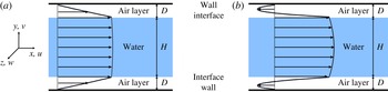
Reference Seo, García-Mayoral and Mani2015). The flow geometry is shown in figure 1, where
 $H$
is the water height and
 $D$
is the air-layer thickness. We fix
 $H$
and vary
 $D$
to match the experimental conditions where the SHS is flush-mounted.
Flow geometry: (a) case 1 (
 ${\it\Pi}_{g}=0$
; shear-driven flow type in the air layer); (b) case 2 (
 ${\dot{m}}_{g}=0$
; recirculating flow type in the air layer). Here,
 ${\it\Pi}_{g}$
is the source term for driving air flow and
 ${\dot{m}}_{g}$
is the mass flow rate within the air layer.

The governing equations for the DNS are the unsteady incompressible Navier–Stokes and continuity equations:
 $$\begin{eqnarray}\displaystyle & \displaystyle {\it\rho}_{{\it\varphi}}\left(\frac{\partial u_{i}}{\partial t}+\frac{\partial }{\partial x_{j}}u_{i}u_{j}\right)=-\frac{\partial p}{\partial x_{i}}+{\it\mu}_{{\it\varphi}}\frac{\partial ^{2}u_{i}}{\partial x_{j}\partial x_{j}}+{\it\Pi}_{{\it\varphi}}{\it\delta}_{1i}, & \displaystyle\end{eqnarray}$$
 $$\begin{eqnarray}\displaystyle & \displaystyle \frac{\partial u_{i}}{\partial x_{i}}=0, & \displaystyle\end{eqnarray}$$
where
 $t$
is the time,
 $x_{i}$
are the coordinates,
 $u_{i}$
are the corresponding velocity components,
 $p$
is the pressure,
 ${\it\rho}_{{\it\varphi}}$
and
 ${\it\mu}_{{\it\varphi}}$
are the density and viscosity of water or air respectively, and
 ${\it\Pi}_{{\it\varphi}}$
is the source term for driving the water or air flow. The subscript
 ${\it\varphi}$
denotes water (
 ${\it\varphi}=l$
) or air (
 ${\it\varphi}=g$
), and the subscript
 $i$
denotes the streamwise (
 $i=1$
or
 $x$
), wall-normal (
 $i=2$
or
 $y$
) or spanwise (
 $i=3$
or
 $z$
) direction. The working fluid properties are
 ${\it\rho}_{l}=998~\text{kg}~\text{m}^{-3}$
,
 ${\it\rho}_{g}=1.2~\text{kg}~\text{m}^{-3}$
,
 ${\it\mu}_{l}=1.0\times 10^{-3}~\text{Pa}~\text{s}$
and
 ${\it\mu}_{g}=1.8\times 10^{-5}~\text{Pa}~\text{s}$
. Here,
 ${\it\Pi}_{l}$
is the mean pressure gradient necessary to drive the water flow with a fixed mass flow rate;
 ${\it\Pi}_{g}$
is the forcing term to determine the air-layer flow: in case 1 (shear-driven flow),
 ${\it\Pi}_{g}$
is zero, whereas in case 2 (recirculating flow with zero net mass flow rate,
 ${\dot{m}}_{g}=0$
),
 ${\it\Pi}_{g}$
is determined by the shear stresses at the wall and interface as (derived from
 $x$
-momentum balance and
 ${\dot{m}}_{g}=0$
inside the air layer)
 $$\begin{eqnarray}{\it\Pi}_{g}=-\frac{{\it\mu}_{g}}{D}\left|\left(\frac{\partial \bar{u}_{g}}{\partial y}\right)_{wall}-\left(\frac{\partial \bar{u}_{g}}{\partial y}\right)_{s}\right|,\end{eqnarray}$$
where the subscript
 $s$
denotes the interface.
The computations are carried out by maintaining a constant mass flow rate in water flow at a Reynolds number of
 $Re=u_{b}H/{\it\nu}_{l}=5600$
 $(Re_{{\it\tau}_{o}}=u_{{\it\tau}_{o}}(H/2)/{\it\nu}_{l}\approx 180)$
, where
 $u_{b}$
is the water bulk velocity,
 $u_{{\it\tau}_{o}}$
is the wall-shear velocity of no-slip channel flow and
 ${\it\nu}_{l}$
is the kinematic viscosity of water. For the time advancement, a third-order Runge–Kutta method for convection terms and the Crank–Nicolson method for diffusion terms are used. A second-order central difference scheme is used for spatial derivatives. Periodic boundary conditions are used in the streamwise and spanwise directions, and the no-slip condition is applied to both the upper and lower walls. While the air–water interface is assumed to be flat, the wall-parallel velocities and shear stresses are maintained to be continuous across the interface. A computational domain of
 $3H\times (H+2D)\times 1.5H$
is used in the streamwise, wall-normal and spanwise directions respectively, with
 $128\times (129+24\sim 80)\times 128$
grids. Uniform grids are used in the streamwise and spanwise directions, while non-uniform grids are used in the wall-normal direction. All simulations are started from a fully developed turbulent channel flow with no-slip walls. The air-layer thicknesses (
 $D$
) considered are from
 $0.0002H$
to
 $0.05H$
. The initial turbulent flow becomes laminar for
 $D\geqslant 0.005H$
(case 1) and
 $D\geqslant 0.02H$
(case 2), so cases up to
 $D<0.005H$
(case 1) and
 $D<0.02H$
(case 2) are discussed in this paper.
3 Results and discussion
3.1 Mean slip length and skin-friction reduction
The mean slip length is obtained from
 $\bar{b}=\bar{u}_{s}/(\partial \bar{u}_{l}/\partial y)_{s}$
, where
 $\bar{u}_{s}$
is the mean slip velocity and
 $(\partial \bar{u}_{l}/\partial y)_{s}$
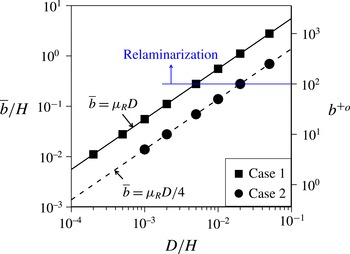
is the mean velocity gradient of the water at the interface. Figure 2 shows the variation of the mean slip length with the air-layer thickness. For both cases 1 and 2, the mean slip lengths linearly increase with the air-layer thickness and their slopes are
 ${\it\mu}_{R}$
and
 ${\it\mu}_{R}/4$
respectively, where
 ${\it\mu}_{R}$
is the viscosity ratio (
 ${\it\mu}_{R}={\it\mu}_{l}/{\it\mu}_{g}$
). At a given air-layer thickness, more slip is induced by the shear-driven air flow (case 1) than by the recirculating air flow (case 2). It is interesting to note that the mean slip length of turbulent flow is the same as that of laminar flow. This counterintuitive result can be explained by the definition of the mean slip length. The mean slip length is rewritten as
 $\bar{b}={\it\mu}_{R}\bar{u}_{s}/(\partial \bar{u}_{g}/\partial y)_{s}$
by matching the shear stresses at the air–water interface. When the velocity profiles inside the air layer are linear (case 1) and quadratic (case 2) functions, the
 $(\partial \bar{u}_{g}/\partial y)_{s}$
values are
 $\bar{u}_{s}/D$
and
 $4\bar{u}_{s}/D$
for cases 1 and 2 respectively. Then, the slip length depends only on
 ${\it\mu}_{R}$
and
 $D$
, independent of the flow condition in water. The mean velocity profiles of the air layer are indeed linear and quadratic for cases 1 and 2 respectively (see below). The slip length in the viscous wall unit (
 $b^{+_{o}}=\bar{b}u_{{\it\tau}_{o}}/{\it\nu}_{l}$
) in figure 2 shows that relaminarization starts when
 $b^{+_{o}}\geqslant 100$
in both cases. This is consistent with the observation by Busse & Sandham (Reference Busse and Sandham2012).
Variation of the mean slip length with the air-layer thickness: symbols, turbulent flow; lines, laminar flow.

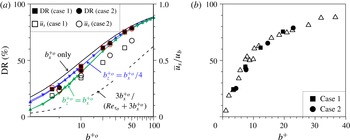
Variations of the DR rate (▪, ●) and the mean slip velocity (▫, ○) with the mean slip length normalized by (a)
 $u_{{\it\tau}_{o}}$
and
 ${\it\nu}_{l}$
and (b)
 $u_{{\it\tau}}$
(shear velocity at the interface) and
 ${\it\nu}_{l}$
. In (a), the solid black, green and blue lines are the DR rates by empirical formulae: lines with triangles, Fukagata et al. (Reference Fukagata, Kasagi and Koumoutsakos2006); lines with inverse triangles, Busse & Sandham (Reference Busse and Sandham2012). The red open rectangles (case 1) and circles (case 2) denote the DR rates from DNS with the present slip-velocity model, (3.1) and (3.2), without solving the air layer. The dashed line in (a) is the DR rate and normalized slip velocity of laminar flow. In (b), the open triangles are the DNS results from various idealized SHSs (Park Reference Park2015).

Figure 3(a) shows the variation of the DR rate and the mean slip velocity with the mean slip length normalized by
 $u_{{\it\tau}_{o}}$
and
 ${\it\nu}_{l}$
, where the DR rate is defined as
 $DR=({\it\Pi}_{o}-{\it\Pi}_{l})/{\it\Pi}_{o}$
;
 ${\it\Pi}_{o}$
is the mean pressure gradient with the no-slip wall. As the mean slip length increases (i.e. as
 $D$
increases), the DR rate and slip velocity also increase. Although the mean slip length remains the same for laminar and turbulent flows, the DR rates in turbulent flows are larger than that in laminar flow and they are even larger than the normalized mean slip velocity. This is because the DR of turbulent flow is determined by the combination of the pure slip effect and the weakening of near-wall turbulence (Park et al.
Reference Park, Park and Kim2013; Rastegari & Akhavan Reference Rastegari and Akhavan2015). The present DR rate falls in between the empirical formulae for the streamwise slip only (
 $b_{z}=0$
, Fukagata et al.
Reference Fukagata, Kasagi and Koumoutsakos2006) and isotropic slip (
 $b_{x}=b_{z}$
, Fukagata et al.
Reference Fukagata, Kasagi and Koumoutsakos2006, Busse & Sandham Reference Busse and Sandham2012), indicating (see below) that the present idealized SHS with an air layer generates an anisotropic slip (
 $b_{x}\neq b_{z}$
), and more slip in the streamwise direction than in the spanwise one (
 $b_{x}>b_{z}$
). Figure 3(b) shows the variation of the DR rate with the mean slip length normalized by the shear velocity at the air–water interface,
 $u_{{\it\tau}}$
, together with the results from Park (Reference Park2015). As indicated by Park et al. (Reference Park, Park and Kim2013), the DR rate correlates well with the mean slip length in the viscous wall unit, irrespective of the flow type inside the air layer and the SHS geometry.
3.2 Anisotropic slip at the air–water interface
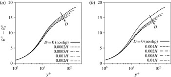
Figure 4 shows the modified mean velocity profiles in the viscous wall unit,
 $\bar{u}^{+}-\bar{u}_{s}^{+}$
, except inside the air layer, where
 $y^{+}=0$
is the location of the air–water interface. As the air-layer thickness increases, the modified mean velocity shifts downward in the buffer and log layers (note that the mean velocity itself shifts upwards with increasing air-layer thickness). Min & Kim (Reference Min and Kim2004) reported that these mean velocities fall on one curve for streamwise slip only, but show downward shifts for combined streamwise and spanwise slip, indicating that the present interface has non-negligible spanwise slip. Hahn et al. (Reference Hahn, Je and Choi2002) showed for turbulent flow over a permeable wall that the downward shift in the modified mean velocity in the buffer and log layers is the result of the decrease in the viscous sublayer thickness.
Modified mean velocity (
 $\bar{u}^{+}-\bar{u}_{s}^{+}$
) profiles in the viscous wall unit: (a) case 1; (b) case 2.

Joint probability density function of
 $u_{s}$
versus
 $(\partial u_{l}/\partial y)_{s}$
: (a–c) case 1; (d–f) case 2; (a)
 $D=0.0002H$
, (b)
 $D=0.0005H$
, (c)
 $D=0.001H$
, (d)
 $D=0.001H$
, (e)
 $D=0.002H$
, (f)
 $D=0.005H$
. The contour levels are from 0.005 to 0.045 in increments of 0.005. The solid and dashed lines have slopes of 1 and
 $1/4$
respectively. The solid circles denote the mean values of the slip velocity and streamwise velocity gradient.

Joint probability density function of
 $w_{s}$
versus
 $(\partial w_{l}/\partial y)_{s}$
: (a–c) case 1; (d–f) case 2; (a)
 $D=0.0002H$
, (b)
 $D=0.0005H$
, (c)
 $D=0.001H$
, (d)
 $D=0.001H$
, (e)
 $D=0.002H$
, (f)
 $D=0.005H$
. The contour levels are from 0.05 to 0.45 in increments of 0.05. The solid and dashed lines have slopes of 1 and
 $1/4$
respectively.

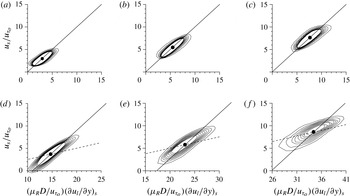
To further investigate the nature of the slip at the interface, we examine the relation between the slip velocity and the velocity gradient at the interface. Figure 5 shows the joint probability density functions (PDFs) between the instantaneous streamwise slip velocity and the velocity gradient at the interface for both cases. The slope between these two (normalized) variables is near 1 for both cases 1 and 2, although this slope becomes lower for larger
 $D/H$
. These results mean that
 $u_{s}\sim {\it\mu}_{R}D(\partial u_{l}/\partial y)_{s}$
or
 $b_{x}\sim {\it\mu}_{R}D$
for both cases. This result is surprising, because the mean slip lengths for cases 1 and 2 are
 $\bar{b}={\it\mu}_{R}D$
and
 $(1/4){\it\mu}_{R}D$
(or
 $\bar{u}_{s}={\it\mu}_{R}D(\partial \bar{u}_{l}/\partial y)_{s}$
and
 $\bar{u}_{s}=(1/4){\it\mu}_{R}D(\partial \bar{u}_{l}/\partial y)_{s}$
) respectively (see figure 2). As shown in figure 5 (solid circles), the slip lengths between the mean slip velocities and the mean velocity gradients hold for the present two cases in terms of joint PDF. The present results clearly indicate that the slip length used for the mean slip velocity and interface velocity gradient should not be applied to instantaneous ones (or fluctuating quantities). Rather, for the two cases considered here, the slip length of
 $b_{x}={\it\mu}_{R}D$
should be applied to the fluctuating components. Thus, the instantaneous streamwise slip velocity may be modelled as (unless the DR rate is very large)
 $$\begin{eqnarray}u_{s}=\left\{\begin{array}{@{}ll@{}}\displaystyle {\it\mu}_{R}D\left(\frac{\partial u_{l}}{\partial y}\right)_{s}\quad & \text{for case 1},\\ \displaystyle {\it\mu}_{R}D\left(\frac{\partial u_{l}}{\partial y}\right)_{s}-\frac{3}{4}{\it\mu}_{R}D\left(\frac{\partial \bar{u}_{l}}{\partial y}\right)_{s}\quad & \text{for case 2}.\end{array}\right.\end{eqnarray}$$
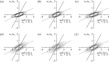
Figure 6 shows the joint PDFs between the instantaneous spanwise slip velocity and the velocity gradient at the interface for both cases, where the mean spanwise velocity is zero. From this result, the instantaneous spanwise slip velocity is modelled as
 $$\begin{eqnarray}w_{s}=\frac{1}{4}{\it\mu}_{R}D\left(\frac{\partial w_{l}}{\partial y}\right)_{s}\quad \text{for cases 1 and 2,}\end{eqnarray}$$
and
 $b_{z}={\it\mu}_{R}D/4$
. Thus, the slip effect in the spanwise direction is much weaker than that in the streamwise direction. The reason why the slip lengths for the streamwise and spanwise fluctuating velocities are different from each other is examined in § 3.3.
The present slip-velocity model, (3.1) and (3.2), provides the anisotropic slip-length relation of
 $b_{z}=b_{x}/4$
. The DR rates versus the slip length with
 $b_{z}=b_{x}/4$
(using the formulae by Fukagata et al. (Reference Fukagata, Kasagi and Koumoutsakos2006) and Busse & Sandham (Reference Busse and Sandham2012)) are plotted in figure 3(a), showing excellent agreement with the present simulation results of case 1 but slight overprediction for case 2. We also perform separate DNS with the present model as the slip boundary conditions (without solving the air layer) and provide the results in figure 3(a). As shown, the present slip-velocity model successfully predicts the drag changes.
3.3 Flow structures in air and water
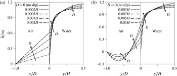
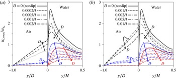
Figure 7 shows the mean velocity profiles in air and water for cases 1 and 2. As mentioned before, the mean velocity profiles inside the air layer are linear (case 1) and quadratic (case 2). With increasing air-layer thickness, the mean velocity in water increases near the interface due to the increased slip velocity but decreases near the centreline to maintain the same mass flow rate inside the channel. Figure 8 shows the r.m.s. velocity fluctuations normalized by
 $u_{{\it\tau}_{o}}$
. The r.m.s. velocity fluctuations are significantly reduced in the water flow for both cases as the air-layer thickness increases. At the air–water interface, for case 1, the streamwise velocity fluctuations increase but the spanwise velocity fluctuations first increase and then decrease with increasing air-layer thickness, whereas for case 2, both the streamwise and spanwise velocity fluctuations first increase and then decrease.
Mean velocity profiles in air and water: (a) case 1; (b) case 2.

Profiles of the r.m.s. velocity fluctuations normalized by
 $u_{{\it\tau}_{o}}$
: (a) case 1; (b) case 2. Black lines,
 $u_{rms}$
; red lines,
 $v_{rms}$
; blue lines,
 $w_{rms}$
.

The results shown in figures 5 and 6,
 $b_{x}={\it\mu}_{R}D$
and
 $b_{z}={\it\mu}_{R}D/4$
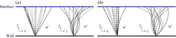
, indicate that the profiles of the streamwise and spanwise velocity fluctuations inside the air layer are more like linear and quadratic respectively, regardless of the cases considered here. In figure 9, we plot some of the instantaneous streamwise and spanwise velocity fluctuations inside the air layer from the present simulations. This figure clearly shows that the profiles of the streamwise velocity fluctuations are very different from those of the spanwise velocity fluctuations, and the first are more like linear but the latter are quadratic. This is because the streamwise velocity fluctuations at the interface have dominant low-frequency components originated from the near-wall streak, but the spanwise ones do not (see the solutions of Stokes’ second problem between two parallel plates for low- and high-frequency oscillations; Sir Lamb (Reference Lamb1916)).
Profiles of the instantaneous velocity fluctuations (
 $u^{\prime }$
and
 $w^{\prime }$
) inside the air layer at every eighth grid point: (a) case 1 (
 $D/H=0.0005$
); (b) case 2 (
 $D/H=0.002$
).

Table 1 shows the Reynolds numbers based on the shear velocities at the interface in air and water respectively, where the Reynolds numbers in air flow are defined as
 $Re_{{\it\tau}}=u_{{\it\tau}}D/{\it\nu}_{g}$
(case 1) and
 $u_{{\it\tau}}(D/2)/{\it\nu}_{g}$
(case 2) respectively. It is notable that the Reynolds numbers in air flow are very small for all of the cases considered. Therefore, turbulence in air flow hardly survives and dissipates although it is continuously supplied at the interface from water flow.
Reynolds numbers based on the shear velocities in air and water.

4 Conclusions
In the present study, we investigated the effects of the air layer on the slip length and skin-friction reduction. Two different flow types inside the air layer were considered: a shear-driven flow and a recirculating flow with zero net mass flow rate. For this purpose, the flow inside the air layer underneath the water turbulent flow was directly simulated with the surface tension neglected. The slip length, slip velocity and drag reduction rate increased as the air-layer thickness increased. At a given air-layer thickness, the shear-driven flow in the air layer supplied more slip than the recirculating flow. However, when the slip length was the same, there seemed to be no clear difference in the drag reduction rate and slip velocity between the two cases. The present drag reduction rate fell in between those from the streamwise slip only and isotropic slip, indicating that the present air–water interface generates an anisotropic slip (stronger in the streamwise slip than in the spanwise one). It was shown that the Navier slip model should be applied to mean values only, and not to instantaneous (or fluctuating) quantities. In this regard, we proposed a new slip model ((3.1) and (3.2)) that provides more slip in the streamwise direction than in the spanwise direction, and showed the validity of this model by separate DNS. Finally, the r.m.s. velocity fluctuations in the water flow were significantly weakened by the air layer, but unsteady motions still existed inside the air layer.
The present study considered ideal circumstances (i.e. no texture on the SHS and a flat air–water interface). In reality, the interface is sustained by the surface tension from the edges of the SHS texture, and is curved and moves due to air dissolution and turbulent pressure fluctuations. Thus, the next step is to apply an interface tracking method such as the level-set or volume-of-fluid method to include the dynamics of the interface due to turbulent pressure fluctuations and examine its relation to the drag reduction capability. This important subject is to be investigated in the near future.
Acknowledgement
This work was supported by the NRF programmes (2011-0028032, 2012M2A8A4055647 and 2014M3C1B1033848) of MSIP, Korea.