



1. Introduction
The flow over a solid flat plate normal to a steady stream is a canonical problem in fluid mechanics. However, many bodies in nature and engineering which are flat are not solid throughout, and the flows they produce in transient environments can produce unique physics. Examples in nature include bird wings (Müller & Patone Reference Müller and Patone1998), soft corals such as the sea fan Gorgonia ventalina, clusters of trees (Bitog et al. Reference Bitog, Lee, Hwang, Shin, Hong, Seo, Mostafa and Pang2011) and human hands during swimming (Matsuuchi et al. Reference Matsuuchi, Miwa, Nomura, Sakakibara, Shintani and Ungerechts2009; Minetti et al. Reference Minetti, Machtsiras and Masters2009; van Houwelingen et al. Reference van2017). Wind turbines and propellers are classic examples of engineered systems which can be modelled as porous plates (e.g. actuator disks), alongside perforated heaving plates (Tao & Dray Reference Tao and Dray2008; An & Faltinsen Reference An and Faltinsen2013; Mentzoni & Kristiansen Reference Mentzoni and Kristiansen2019), sports rackets (Huera-Huarte Reference Huera-Huarte2013) and breakwaters (Li et al. Reference Li, Liu and Li2024).
Major theoretical work on perforated plates placed normal to a steady flow can be traced back to the application of an actuator disk model to wind turbines by Betz (Reference Betz1920). The connection between actuator disk theory and perforated plates comes by way of the open area fraction of the plate, as this is predominantly what is used to characterise their resistance. The open area fraction is the ratio of open area of the plate to the total plate area:
 $\beta \equiv ( {A_{open}}/{A_T})$
,
 $0\leqslant \beta \leqslant 1$
, so
 $\beta =0$
for a solid plate and
 $\beta =1$
for a plate which does not disturb the flow in any way. A distributed point-source model was used by Taylor (Reference Taylor1944) in an investigation of porous screen drag. These early models only worked when the momentum deficit was small (
 $\beta \approx 1$
), since they do not account for mixing, nor does the Taylor (Reference Taylor1944) model conserve mass. Subsequently, Koo & James (Reference Koo and James1973) introduced a model in which the streamfunction is scaled down in the wake region so as to conserve mass. Although the model of Koo & James (Reference Koo and James1973) is an improvement since it does not account for mixing, it too only works for
 $\beta \approx 1$
. By introducing an unknown base pressure, and conserving mass, momentum and energy in order to find this pressure Steiros & Hultmark (Reference Steiros and Hultmark2018) improved upon the model of Koo & James (Reference Koo and James1973), since the base pressure accounts for mixing. Their model is able to predict experimentally measured developed flow drag generated by perforated plates for large
 $\beta$
, and when a splitter plate is used to suppress von Kármán vortex shedding they get good agreement for small
 $\beta$
too.
In a seminal experimental work, Castro (Reference Castro1971) studied the effect of
 $\beta$
on the fluid forces and wake dynamics once the flow was fully developed. The investigation revealed that there exists a recirculation bubble in the mean flow behind a perforated plate which moves away from the plate and shrinks in size as
 $\beta$
is increased from
 $0$
, until it eventually disappears. The von Kármán vortex shedding, which occurs for
 $\beta =0$
, ceases to exist above a critical value of
 $\beta$
. A defining feature of developed flows past a perforated flat plate is that the drag decreases when more flow goes through the plate. It was remarked that, in this way, the flow moving through the plate’s holes acts akin to a splitter plate. Recent work by Cicolin et al. (Reference Cicolin, Chellini, Usherwood, Ganapathisubramani and Castro2024) produced a more complete picture of the shedding by using particle image velocimetry (PIV). They also used correlations between hot-wire time series to discover an intermediate regime,
 $\beta \in (0.22,0.3)$
, where shedding is intermittent.
Unsteady vortex formation processes behind a solid plate have been studied extensively in two dimensions using inviscid analytic theory (Kaden Reference Kaden1931; Rott Reference Rott1956; Pullin Reference Pullin1978; Cortelezzi & Leonard Reference Cortelezzi and Leonard1993), inviscid point-vortex codes (Kuwahara & Takami Reference Kuwahara and Takami1973; Sarpkaya Reference Sarpkaya1975; Dutta Reference Dutta1988; Chein & Chung Reference Chein and Chung1988) and with viscous simulations (Chua Reference Chua1990; Cortelezzi Reference Cortelezzi1995; Koumoutsakos & Shiels Reference Koumoutsakos and Shiels1996; Wang & Eldredge Reference Wang and Eldredge2012; Xu & Nitsche Reference Xu and Nitsche2015). The analytic inviscid two-dimensional (2-D) models capture well the early-time (these models work well only when the plate has moved much less than the length of its chord, while executing a power-law motion) behaviour (Pullin & Perry Reference Pullin and Perry1980), and predict self-similar growth in the shape and strength of the nascent vortex at each edge of the plate. The single variable-strength point-vortex model of Rott (Reference Rott1956) obtains the correct growth behaviour, whereas the more sophisticated vortex-sheet model of Pullin (Reference Pullin1978) captures the structural aspects which were missed. The aforementioned viscous simulations have been able to capture the flow phenomena which are present up to moderate times (i.e. while the wake has yet to show alternating-sign vortex shedding, for
 $\beta$
where this is known to eventually occur, and time-average quantities have yet to settle to their final values) at low Reynolds numbers as compared with, for instance, the experiments of Taneda & Honji (Reference Taneda and Honji1971). However, it was shown experimentally that it can take 30 or more chord lengths for von Kármán vortex shedding to first appear (Lisoski Reference Lisoski1993), and much longer still for the flow to fully develop. The author further suggested the reason no 2-D simulation, inviscid or viscous, could match the experimentally known value of drag is intrinsic three-dimensional (3-D) flow effects, which they were able to mostly suppress using density stratification.
Thus far, work on unsteady perforated plate fluid dynamics has been largely application-specific. Much work has been done to understand heaving plates, where the focus has been on experimentally measuring, or numerically modelling, the added mass effect as a function of the dimensionless frequency known as the Keulegan–Carpenter number (Tao & Dray Reference Tao and Dray2008; An & Faltinsen Reference An and Faltinsen2013; Mentzoni & Kristiansen Reference Mentzoni and Kristiansen2019). In sports science, it was noticed in many studies that steady drag increases slightly when a swimmer’s fingers are spread slightly (e.g. Minetti et al. Reference Minetti, Machtsiras and Masters2009). However, unsteady lift and drag forces were argued to play an important role in human swimming (Matsuuchi et al. Reference Matsuuchi, Miwa, Nomura, Sakakibara, Shintani and Ungerechts2009), and some studies have even quantified the effect of finger spread on unsteady drag forces (Bihan Reference Bihan2020). This latter study builds on the results found in Grift et al. (Reference Grift, Vijayaragavan, Tummers and Westerweel2019) in which drag on a rowing-oar-like plate accelerated through the water’s surface showed a drag peak at the end of acceleration, a transition phase and finally a steady phase. The authors proposed that drag in this situation is best split into added-mass-like and steady-drag terms in order to handle the complexities of the situation.
In this background of extensive work on steady flow on perforated plates, unsteady flow on solid plates and application-specific work on unsteady flow on perforated plates, fundamental studies of unsteady flow on perforated plates are lacking. The inviscid point-vortex modelling work of Inoue (Reference Inoue1985) is a notable exception, although that model depends on a porosity parameter which was not connected back to the geometry of the perforation or porosity. In our study, we experimentally investigate how perforated plate open area fraction affects the development of the flow and forces when a plate is undergoing nearly impulsive motion. We close the model of Inoue (Reference Inoue1985), and compare with our experimental results, enabling both physical insight and predictive capability. Due to the constraints imposed by the length of our facility, we focus on times early in the starting flow development (during the time the plate moves a distance of 8 chord lengths), so the wake is largely symmetric.
2. Methods
2.1. Perforated plate
Our test model was constructed from a standard 0.95 mm thick perforated plate with 3.97 mm hole size and 4.76 mm centre-to-centre hole distance, set flush in a custom machined rectangular aluminium frame (the upstream-pointing face of the model is flat). The perforated steel plate provides an open area fraction,
 $\gamma$
, of 63 % on the perforated portion. The frame stiffens the model and provides a clean edge along which the flow separates. The frame is
 $2.95\,\text{mm}$
thick, with
 $30^\circ$
knife-edge along the upper and lower edge of the plate. The span of the frame is
 $l=315\,\text{mm}$
, and the height is
 $c=61\,\text{mm}$
. The test subject is shown in figures 1 and 2. The solid frame constitutes
 $p=19.8\,\,\%$
of the model’s area, so the open area fraction of the plate as a whole is
 $\beta =(1-p)\gamma$
. Arbitrary values of
 $\beta$
are achieved by affixing a mask to the front of the perforated portion of the plate. By entirely blocking some holes while keeping others completely unobstructed, the mask allows any value of
 $\beta$
to be achieved up to
 $\beta = 50.5\,\%$
. The mask is constructed of laser-cut transparency film. It is aligned with the hole pattern using machined reference pins, and fixed in place with a thin strip of tape along the edges of the mask. Frontal views of the plate with the various masks affixed are shown in figure 1(a–n). In these figures white areas represent places fluid can flow through while black areas block the flow. Figure 1(o) shows a cross-section view of the plate along with various relevant dimensions. The downward-sloping cross-hatched regions represent the frame, the upward-sloping cross-hatched regions represent the perforated metal section and the solid regions represent the mask.
Perforated plate model frontal view with solid mask (a), as well as
 $\beta =\{4\,\%,8\,\%,12\,\%, 16\,\%,20\,\%,24\,\%,28\,\%,32\,\%,36\,\%,40\,\%,44\,\%,48\,\%,50.5\,\%\}$
shown in (b–n), respectively. The white area is open to the flow while the black area blocks the flow. A labelled cross-section view, with measurements shown in millimetres (o).

Test subject side view (left). Separation bubble has a size of
 $s$
chords. Frontal view of test subject (right).

The masks are generated deterministically on the computer by covering holes successively, while maintaining homogeneity and starting with a completely open mask, until the desired value of
 $\beta$
is achieved. The 4 : 1 hole aspect ratio of the perforated section is expected to make our results representative of a zero-thickness perforated plate (Smith & Van Winkle Reference Smith and Van Winkle1958), and the fact that hole size is kept constant across
 $\beta$
ensures hole Reynolds number is fixed.
2.2. Flow facility
Experiments were conducted by translating the perforated plates, normal to their front face, through a water tank with test section dimensions of
 $1.2\,\mathrm{m} \times 0.6\,\mathrm{m} \times 0.6\,\mathrm{m}$
(length
 $\times$
width
 $\times$
height), corresponding to a blockage ratio of 5.3 %. The plate’s centre was positioned
 $0.32\,\mathrm{m}$
below the water surface. Motion was prescribed using a custom belt-driven gantry, with position, velocity and acceleration measured via the internal rotary encoders of the gantry’s motors (ClearPath, Teknic, USA) fused with an accelerometer (ADXL354, Analog Devices, USA) using Kalman smoothing. The velocity profile was piecewise linear: a constant-acceleration phase over a distance of
 $c/4$
, followed by constant velocity
 $U_f = 7.5\,\mathrm{cm\,s}^{-1}$
to reach a total travel of
 $0.5\,\mathrm{m}$
. Space constraints prevented longer runs, and complete flow development is known to take much longer for solid plates (Lisoski Reference Lisoski1993). Therefore, the flows in this experimental campaign are expected to be transient and not fully developed. The time to complete development is not known for other cases, so there may be value in future studies with a longer tow tank. The constant-velocity phase corresponds to a chord Reynolds number of
 $Re\equiv (({cU_f})/{\nu })=4900$
, and a hole Reynolds number of
 $Re_h\equiv (( {\text{d}U_f})/{\nu })=320$
. Throughout this paper we will be using the dimensionless time known as the formation time,
 $T$
, since
 $T$
is known to be more relevant to vortex formation processes than time itself,
 $t$
, in general (Gharib et al. Reference Gharib, Rambod and Shariff1998) and for flat plates in particular (Taneda & Honji Reference Taneda and Honji1971). It can be shown that the formulation of Gharib et al. (Reference Gharib, Rambod and Shariff1998) is equivalent to
 \begin{equation} T\equiv \frac {1}{c}\int _0^t U(\tau )\,\text{d}\tau , \end{equation}
where
 $U(t)$
is the plate’s velocity as a function of time. In this representation, formation time happens to be the distance moved by the plate normalised by the length of its chord. Position and velocity tracking errors remained below
 $200\,{\unicode[Arial]{x03BC}}\mathrm{m}$
throughout the motion and below
 ${\sim} 30\,{\unicode[Arial]{x03BC}} \mathrm{m}$
during the constant-velocity phase, which resulted in acceptable velocity errors (see velocity trace, figure 3). Drag force was measured using a six-axis force transducer (Delta IP65, ATI Industrial Automation, USA). The plate was mounted to the sensor via acrylic supports, which also served as end-plates (
 $3.175\,\mathrm{mm}$
thick). A side view of one of the plates is shown in figure 2. Because the measured force includes inertial effects from gantry accelerations, vibrations and linear rail curvature, each measured force trace is subtracted by the force measured from identical motion with the plate removed but its mass replaced above the waterline. Force readings were tared immediately before motion began to minimise sensor drift.
Three trials were performed for each level of perforation. Between trials, and after changing perforation levels, the water was left to settle to a root-mean-square flow velocity of roughly 1–2 mm s−1 (or less).
Plate velocity trace as measured by the gantry’s sensors (black line), and target velocity (blue line).

Experimental set-up. The perforated plate is dragged by a gantry through the test section. Cameras capture the motion of particles, illuminated by a laser, at centre plane. Reproduced from (Bollt, Foxman & Gharib Reference Bollt, Foxman and Gharib2025) with permission of the authors.

2.3. Particle image velocimetry set-up
The flow was illuminated from behind the plate at centre plane by a 450 nm 10 W laser expanded by a cylindrical lens and steered by a submerged mirror. Seeding was provided by 13
 ${\unicode[Arial]{x03BC}} \mathrm{m}$
nominal diameter silver-coated glass microspheres (Conduct-O-Fil SH400S20, Potters Industries, USA). Images were taken at 100 Hz with three synchronised high-speed cameras (XSM-3520, Integrated Design Tools, USA) (
 $f=$
32 mm,
 $f/1.15$
lens) aligned perpendicular to the laser plane. The images were unwarped and stitched together into a single 1391 × 4999 px2 image using a 1 cm grid calibration target such that no occluded region exists throughout the plate’s motion. Intensity matching across the stitched region was enforced via contrast-limited adaptive histogram equalisation and high-pass spatial filtering. The particle concentration was roughly 0.02 particles per pixel. Velocity fields were generated using commercial PIV software (PIVview2C, PIVTEC GmbH, Germany). Multi-grid evaluation with 16 px window size (uniformly weighted windows), 50 % overlap and correlation-plane summing using nine slightly displaced planes (see Hart Reference Hart2000) were used. The calibration is
 $4492\ \text{px m}^{-1}$
, so the resolution is 3.6 mm based on the window size. Universal outlier detection and correlation-coefficient thresholding were applied. Outliers were replaced via interpolation. The random error in each velocity vector was measured to have a standard deviation of
 $2\,\%$
of
 $U_f$
(or
 $0.07\,\text{px}$
). Uncertainty from image unwarping is less than 0.2 %.
3. Results
In this section we present the recorded forces, velocity and vorticity fields, wake bubble size and total circulation and effective vortex location in the upper half plane. All of these quantities depend on
 $\beta$
. The plate’s trajectory is maintained invariant by the gantry’s motion controller. The PIV data are recorded from a single run for plates with
 $\beta =\{0\,\%,4\,\%,8\,\%,12\,\%,16\,\%,20\,\%,24\,\%,28\,\%,32\,\%,36\,\%,40\,\%,44\,\%,48\,\%,50.5\,\%\}$
. Force is recorded from the average of three runs, one of them being the run where PIV data are taken, for
 $\beta =\{0\,\%,4\,\%,8\,\%,12\,\%,16\,\%,20\,\%,24\,\%,28\,\%,32\,\%,50.5\,\%\}$
.
In what follows, whenever both a dimensional and dimensionless version of a variable exists, we distinguish them by using a prime to denote the dimensional version (e.g.
 $\omega '$
for dimensional vorticity and
 $\omega$
for dimensionless vorticity).
3.1. Forces
We define the drag coefficient as
 \begin{equation} c_d\equiv \frac {D}{\frac {1}{2}\rho A U_f^2}, \end{equation}
where
 $A\equiv cl$
represents the bounding-rectangle’s area. The drag coefficient generated by the plate’s motion, for various values of
 $\beta$
ensemble-averaged over three trials per
 $\beta$
and Gaussian filtered, is shown in figure 5(a). Because of the sharpness of the drag coefficient peak, the amount of smoothing which can be applied to that region of data must be kept to a minimum without producing noise artefacts, since excessive filtering will attenuate the peak. For this reason the Gaussian filtering over the region
 $T\leqslant 0.25$
had a standard deviation of 0.17 s. For the rest of the data, a standard deviation of 0.28 s was used beyond
 $T=2$
, with
 $0.25\leqslant T\leqslant 2$
filtered in an amount linearly between these two extremes. In both cases the filtering was chosen to be just sufficient to attenuate those force fluctuations which were known to be trial- and
 $\beta$
-independent mechanical disturbances. The repeatability between experiments was quite good, as demonstrated by the small spread in the trials in figures 5(a) and 5(b). This means the main source of uncertainty in the measured
 $c_d$
comes from mechanical disturbances.
(a) Plots of
 $c_d$
versus
 $T$
for each
 $\beta$
. Dot-dashed curve: solid plate from Ringuette et al. (Reference Ringuette, Milano and Gharib2007). Dashed curve: high-aspect-ratio solid plate with
 $T\leqslant 0.5$
acceleration phase from Lisoski (Reference Lisoski1993). Thin grey curve: all three trials which make up the mean for
 $\beta =50.5\,\%$
. Inset: same curves, but vertical scale in the range
 $c_d\in [0.7,1.9]$
. (b) Mean solid-area-normalised drag coefficient over
 $T\in [7,8]$
versus perforation (blue stars), and developed flow literature (black symbols). Error bars are maximum and minimum of the three trials. Chord Reynolds numbers from other authors span the range from
 $6 \times 10^3$
to
 $9\times 10^4$
.

For all traces, the same general trend appears. When acceleration commences, the force rises almost instantly to a finite value. The force continues to rise after this until it reaches a maximum at
 $T=1/4$
, which is the time where the plate’s acceleration ceases. From there the force drops towards its final value.
Some qualitative differences between
 $\beta$
arise in the measured forces after acceleration ceases at
 $T=1/4$
. For only the 0 % and 4 % cases the drag drops and then begins to rise slightly by the end of the experiment. The
 $\beta =0\,\%$
drag drops lower than the
 $\beta =4\,\%$
drag (it reaches a minimum of
 $c_d = 1.3$
at
 $T\approx 4$
). This is slightly earlier and less substantial than the minimum measured by Ringuette et al. (Reference Ringuette, Milano and Gharib2007), which is
 $c_d=1.15$
at
 $T\approx 5$
. However, even though their acceleration phase was twice as long in
 $T$
, it agrees with Lisoski (Reference Lisoski1993) on the value of the minimum, but not the timing (
 $T\approx 8$
). The subsequent drag rise for
 $\beta =0\,\%$
reaches
 $c_d=1.8$
, which is slightly higher than Lisoski’s measurement of
 $c_d=1.65$
. These disagreements are not unexpected since Lisoski (Reference Lisoski1993) found that the timing and severity of the rapid rise in force following the drag undershoot are sensitive to things such as blockage ratio, aspect ratio and acceleration profile. These phenomena are also highly sensitive to how normal the plate is to the flow. The fact that after
 $T=1/4$
the drag monotonically drops when
 $\beta \gt 4\,\%$
, but not when
 $\beta \leqslant 4\,\%$
, is noteworthy because it results in a period of roughly
 $T\in [3,5]$
where a solid plate has less drag than a plate with a moderate level of perforation.
It is informative to compare the average drag experienced by each plate over the interval
 $T\in [7,8]$
with the developed flow mean drag measured in the literature. The comparison with developed flow data in figure 5(b) is informative of how much the drag needs to further change between the end of our experiment and when the flow develops completely. The tow tank was not long enough to observe transition to von Kármán vortex shedding in any of our experiments even though for the smaller
 $\beta$
we tested this type of shedding is known to exist in the developed flow state. Thus, in interpreting figure 5(b), the drag-producing mechanism at the end of our experiment should not be assumed to be similar to what it is in developed flow merely because the quantity of drag is fairly similar.
We have chosen to plot drag in terms of
 ${\overline {c_d}}/({1-\beta })$
in figure 5(b), which represents the drag coefficient based on the solid area rather than the area of the bounding rectangle. Doing so brings out an interesting trend in the developed flow data already available in the literature (black symbols), which has not been heretofore noticed to our knowledge: the drag coefficient is nearly invariant with
 $\beta$
when it is expressed in this way, having a value close to 2 for large and small
 $\beta$
, with a minimum of roughly 1.7 for intermediate
 $\beta$
. Although the developed flow drag coefficients measured by others, expressed in this way, are roughly constant it does not imply the drag production mechanism is the same across
 $\beta$
, and indeed it is known not to be, since above a certain
 $\beta$
von Kármán vortex shedding is suppressed (Cicolin et al. Reference Cicolin, Chellini, Usherwood, Ganapathisubramani and Castro2024). The trend does not seem to have any substantial Reynolds number dependence as evidenced by the fact that the data plotted come from a wide range of hole and plate chord Reynolds numbers while this does not appear to explain much of the spread.
Vorticity plot at
 $T = 0.25$
(a,d,g),
 $T=1$
(b,e,h) and
 $T=4$
(c,f,i) for
 $\beta =0\,\%$
(a–c),
 $\beta =24\,\%$
(d–f) and
 $\beta =50.5\,\%$
(g–i). Grey lines: streamlines in the frame of the plate. Black trapezoid: the plate. Black
 $\times$
and
 $+$
: edges of the recirculation bubble along the centreline. The secondary vortices are labelled in (b). Alternating-sign vortices shed behind the plate’s frame are labelled in (h).

Vorticity plot at
 $T = 8$
for
 $\beta =0\,\%, 24\,\%, 50.5\,\%$
in (a–c), respectively). Grey lines: streamlines in the frame of the plate. Black trapezoid: the plate. Black
 $\times$
and
 $+$
: edges of the recirculation bubble along the centreline. Alternating-sign vortices shed behind the plate’s frame are labelled in (c).

3.2. Vorticity and flow structures
The PIV data at perforation levels
 $\beta = \{0\,\%, 24\,\%, 50.5\,\%\}$
are used to generate dimensionless vorticity and streamline plots at time instants
 $T = {0.25, 1, 4, 8}$
, in a plate-fixed reference frame. Vorticity was calculated from the velocity field, based on the Stokes theorem, by calculating the circulation measured on the perimeter of a 3 × 3 square contour (Reuss et al. Reference Reuss, Adrian, Landreth, French and Fansler1989; Landreth & Adrian Reference Landreth and Adrian1990). These results are shown in figures 6 and 7, with the velocity and vorticity data temporally filtered by a Gaussian kernel with standard deviation of 3 frames. The dimensionless vorticity is defined by
 $\omega \equiv \omega ' c/U_f$
. Dimensionless vorticity random error standard deviation is just
 $0.1$
because of the filtering, and the velocity random error standard deviation becomes
 $0.6\,\%$
of
 $U_f$
. At early times, particularly
 $T = 0.25$
, the vorticity fields are nearly symmetric across all
 $\beta$
(compare figures 6
a, 6
d and 6
g), with the shape and location of the Kaden spiral (Kaden Reference Kaden1931) (starting vortex) produced by each edge of the plate largely unaffected by perforation. However, vortex strength decreases as
 $\beta$
increases, as is already apparent in figures 6(a), 6(d) and 6(g). Jetting through hole groups is evident in figure 6(d), although the PIV resolution is insufficient to capture individual jets (hole diameter is of the same order as the PIV grid’s Nyquist wavelength), so non-uniform flow behind the holes when
 $\beta =50.5\,\%$
is not visible (see e.g. figure 6
g). As shown in figures 6(b), 6(e) and 6(h), by
 $T = 1$
the flows remain largely symmetric, but instabilities begin to differentiate the wakes. In the
 $\beta = 0\,\%$
case (figure 6
b), a Kelvin–Helmholtz instability breaks the shear layer feeding the starting vortex into discrete vortices. This behaviour is less pronounced for
 $\beta = 24\,\%$
(figure 6
e), and for
 $\beta = 50.5\,\%$
(figure 6
h) the starting vortex has already pinched off, with a second vortex beginning to form. Due to increased flow through the plate and reduced vortex strength at higher
 $\beta$
, a stagnation point marked with a plus symbol is only visible for the solid plate at
 $T=1$
(figure 6
b). A small, weak, secondary vortex of opposite sign is also visible in figure 6(b). This is a known phenomenon for starting flows near an edge (Rott Reference Rott1956; Pullin & Perry Reference Pullin and Perry1980), steady flow over delta wings (Brown & Michael Reference Brown and Michael1954; Lambourne & Bryer Reference Lambourne and Bryer1961), etc. At
 $\beta =24\,\%$
these secondary vortices are substantially stronger and larger, especially at
 $T=4$
(figure 6
f). These prominent secondary vortices also show up in the mean developed flow data of Cicolin et al. (Reference Cicolin, Chellini, Usherwood, Ganapathisubramani and Castro2024). When
 $\beta =50.5\,\%$
the thin solid frame of the perforated plate (see e.g. figure 1
n) creates a small wake region behind itself as seen in figures 6(h) and 7(c). The flow through the plate is slower than the flow around the plate, so this frame wake is a feature within the shear layer produced by the perforated plate as a whole, akin to combined shear-wake flows observed by Koochesfahani & Frieler (Reference Koochesfahani and Frieler1989).
At later times (
 $T = 4$
and
 $T = 8$
), perforation increasingly alters the wake structure. For the solid plate (figures 6
c and 7
a), the broken shear layer continues to feed the starting vortex with discrete vortices, and has moved away from the line
 $y=0$
. For
 $\beta = 24\,\%$
(figures 6
f and 7
b) the vorticity does not move away from
 $y=0$
to nearly the same degree, but compared with the remarkable symmetry present in figure 6(c) some asymmetry exists in figure 6(f). A coherent starting vortex still exists and generates a distinct recirculation bubble. After examining the vorticity field time series, it becomes clear that the vortex doublet thus formed does not substantially feed on the shear layers the plate is producing but moves between them. By
 $T = 8$
(figure 7
b), the doublet has mostly broken up, though some recirculation persists. When
 $\beta =50.5\,\%$
the discrete vortices shed by the plate’s edges each loosely form a shear layer, with the starting vortex pair formed being the most coherent (see figure 6
i). The first pair of shed vortices slowly get squeezed towards each other so that they form a clear doublet at
 $T=8$
(figure 7
c), although the strength of the flow they produce is not sufficient to form a recirculation bubble in the plate-fixed frame.
In summary, the presence of a recirculation bubble formed by a vortex doublet that feeds on the plate’s shear layers characterises the wake of a solid plate after the vortices generated by each edge of the plate begin to interact but before the wake becomes asymmetric. In contrast, highly perforated plates exhibit two largely non-interacting shear layers with a weak starting vortex at the tip of the shear layer. Intermediate perforation levels produce hybrid behaviour: a vortex doublet forms within a recirculation bubble that travels between the shear layers but interacts with them less as
 $\beta$
increases.
Log–log plot of
 $s$
versus
 $T$
. Dotted black line: fit for solid-plate
 $s(T)$
from Taneda & Honji (Reference Taneda and Honji1971). Black line: stagnation point in mean velocity field for developed flow when
 $\beta =\{0\,\%,12\,\%,16\,\%,28\,\%\}$
, from Cicolin et al. (Reference Cicolin, Chellini, Usherwood, Ganapathisubramani and Castro2024).

The simultaneous presence of doublet-like and shear-layer-like behaviour in the wake of perforated plates leads to distinctive trends in the size and position of the recirculation bubble. We tracked the bubble’s location over time by identifying the two zeros in horizontal velocity along the centreline (in the plate-fixed frame), which mark the inner and outer centreline ‘stagnation points’. The dimensionless distance of the outer stagnation point from the plate is denoted
 $s$
, and is shown schematically in figure 2. Examples are shown in figures 6 and 7 of both stagnation points. After applying a three-point median filter and Gaussian filter (standard deviation: 3 frames) to eliminate a few isolated outliers and smooth the data, the resulting trajectories of the outer stagnation point are plotted in figure 8, alongside the empirical fit proposed by Taneda & Honji (Reference Taneda and Honji1971) for solid plates and the measured location of the stagnation point for developed flow from Cicolin et al. (Reference Cicolin, Chellini, Usherwood, Ganapathisubramani and Castro2024). The Taneda & Honji (Reference Taneda and Honji1971) fit matches our data reasonably well for the solid plate in the range
 $T \in [0.7, 2]$
, but over-predicts the location of the outer stagnation point at both smaller and larger
 $T$
. This discrepancy is not surprising, as their experiments were limited to no greater than
 $Re = 1135$
and the fit was primarily built using smaller-
 $Re$
flows, and only verified at the highest
 $Re$
for data in the domain
 $T \in [0.483, 2.96]$
. Prior numerical studies have also found that the Taneda–Honji fit does not extrapolate reliably outside this range, particularly at higher Reynolds numbers, for both impulsive start (Inoue Reference Inoue1985) and constant acceleration (Koumoutsakos & Shiels Reference Koumoutsakos and Shiels1996).
For perforated plates, the outer stagnation point, marking the bubble’s extent, shifts significantly with increasing
 $\beta$
. As
 $\beta$
increases, the bubble forms later. This trend continues up to
 $\beta = 40\,\%$
. The
 $\beta =40\,\%$
curve is broken in multiple places because the doublet is only just strong enough to form a stagnation point for a short period, so any shift in vorticity in the region can remove the stagnation point (no stagnation location data to show) or reinstate it briefly. Beyond that, no recirculation bubble forms at all since at larger
 $\beta$
the vortex doublet which is responsible for the bubble has become too weak, so there is no stagnation point data to show above
 $\beta =40\,\%$
. This trend is qualitatively similar to that found for the recirculation bubble in the developed-flow mean velocity field measured behind a perforated plate from Cicolin et al. (Reference Cicolin, Chellini, Usherwood, Ganapathisubramani and Castro2024), but the threshold in
 $\beta$
where the recirculation bubble disappears is roughly 10 % higher for starting flow in our study than for developed flow in their study. From figure 8 it can also be seen that for solid plates the location of the developed flow’s stagnation point from Cicolin et al. (Reference Cicolin, Chellini, Usherwood, Ganapathisubramani and Castro2024) is substantially smaller than the value achieved at large
 $T$
in our experiment. However, by
 $\beta =16\,\%$
the developed flow’s stagnation point location has exceeded the value we see at the end of our experiment. In their experiments a maximum was observed in the location of the stagnation point between
 $\beta =16\,\%$
and
 $\beta =28\,\%$
(the same line is used for these two in figure 8 because their values are negligibly different). Meanwhile our experimentally measured stagnation point locations do not appear to have a maximum in
 $\beta$
, so by
 $\beta =28\,\%$
the value achieved at the end of the experiment is nearly as high as the one seen in the developed flow.
3.3. Total circulation and centre of impulse
Circulation is measured separately for the contours enclosing the upper and lower half-planes, and their magnitude is found to agree to better than 5 % (except at early time when circulation is very small), consistent with the expected up–down symmetry of the flow field. The results reported here represent the average of the magnitude of the two circulations in the upper and lower half-planes. The circulation is filtered in time with a Gaussian kernel with standard deviation of 3 frames. During the constant-acceleration period (
 $0\lt T\leqslant 0.25$
), the circulation appears to grow nearly linearly in time for all
 $\beta$
, with a growth rate that decreases with increasing
 $\beta$
(see the linear plot in figure 9
a). Upon least-squares fit to a power-law dependence
 $\varGamma \propto T^g$
at each
 $\beta$
over
 $0 \lt T\leqslant 0.25$
, however, we find the best estimate is
 $g = 0.88\pm 0.12$
over the range of
 $\beta$
studied here (rather than a linear fit, which would be
 $g=1$
). This result is interesting in that, as further discussed in § 4.1, we show that theory predicts a value of
 $g = 5/6 \approx 0.83$
for all
 $\beta$
. After the end of the acceleration period, the solid plate’s total circulation in figure 9(b) appears to follow a power law from
 $T=0.4$
to
 $T=4$
. If we fit a function
 $\varGamma (T,\beta )=a(\beta )T^{b(\beta )}$
to the data in the domain
 $T\in [0.4,4]$
, it becomes clear that both the coefficient
 $a(\beta )$
and exponent of the power law
 $b(\beta )$
change linearly with
 $\beta$
for our data. Namely,
 $a(\beta )=2.63-4.29\beta$
and
 $b(\beta )=0.529+0.740\beta$
(see inset of figure 9 for performance of this fit).
Circulation as a function of
 $T$
. (a) Linear scale. (b) Log–log scale. The inset in (b) shows power-law fit performance: circulation normalised by
 $a(\beta )=2.63-4.29\beta$
versus
 $T^{b(\beta )}$
where
 $b(\beta )=0.529+0.740\beta$
. Dashed black line, with slope 1, included for reference. Coloured dashed lines are extrapolated.

Coefficient (red) and power (blue) of the best-fit power law to the total circulation curve of figure 9 over the domain
 $T\in [0.4,4]$
, plotted as a function of
 $\beta$
. Dashed lines are a linear best fit to the coefficients.

The ‘centre of impulse’ (COI) for vorticity in the wake of a plate in the upper half-plane was tracked to gain insight into the wake and drag force behaviour. The COI is a new way of representing the location of a distribution of vorticity. It is constructed so that if the flow were truly 2-D across the entire plate we could calculate the force on the body exactly from the impulse equation (Saffman Reference Saffman1993) as if the entire vorticity field were condensed into just two point vortices: one vortex for each edge of the plate. The technical details of the construction are given in Appendix A.2, and the mathematical definition is given in (A15), where the sums become integrals when dealing with vorticity fields. (It turns out that in free space the COI is conveniently just the centre of vorticity,
 $\int \omega \underline {x}\text{d}A/\int \omega \text{d}A$
, so it is possible to tell by eye how motion of distributions of vorticity relate to forces using the change in the product of circulation and centre of vorticity. However, in the presence of the plate, the more general definition of COI is required in order to discuss the forces resulting from the motion of distributed vorticity without having to discuss the distribution itself.) We apply temporal filtering to the COI using a Gaussian kernel with a standard deviation of 6 frames.
In figure 11(a) we can see that for small
 $\beta$
and
 $T\lt 2$
the dimensionless COI in the direction normal to the flow,
 $y_{\textit{COI}}\equiv y'_{\textit{COI}}/c$
(where
 $y'_{\textit{COI}}$
is the dimensional COI in the transverse direction), decreases slightly with
 $T$
, but afterwards the COI accelerates outwards, resulting in the COI half a chord above the plate’s tip. At larger
 $\beta$
the acceleration is significantly reduced. In figure 11(b) we see that for
 $T\lt 1$
the COI’s dimensionless horizontal position,
 $x_{\textit{COI}}$
, appears to change little with
 $\beta$
. When
 $T\gt 4$
,
 $x_{\textit{COI}}$
varies linearly with
 $T$
(shown by the dashed trend lines). The slope of
 $x_{\textit{COI}}$
varies linearly with
 $\beta$
while the intercept is independent of
 $\beta$
. These linear trends are well parametrised by
 $x_{\textit{COI}}=(0.13+0.49\beta )T+0.35$
.
(a) Transverse position of upper-half-plane COI, with respect to the upper corner of the plate. (b) Streamwise position of upper-half-plane COI with respect to the plate’s location. The
 $T$
axis starts at
 $T=0.25$
for both panels.

4. Flow modelling
To understand the flow further we use the same 2-D point-vortex flow model as Inoue (Reference Inoue1985). This model is able to reproduce some of the behaviour observed in our experiments and allow us to understand the driving mechanisms in the flow. It turns out that Inoue’s model cannot be used on its own to make comparisons with experiments since, as will be seen, it contains an unspecified constant. We therefore provide an empirical closure model using our experimental data to allow direct comparisons to be made. In this section we discuss the model, method of closure and comparison between the model and experiments. The finer details of the model, necessary for reproduction, can be found in Inoue (Reference Inoue1985) as well as Appendix A.
If the dimensional position of a point in the complex plane is
 $z'\equiv x'+y'{\rm i}$
, Inoue’s model approximates the flow as a linear combination of the complex potential for the flow past a solid plate,
 $f'_{s}(z')$
, a uniform flow through it and a system of point vortices and their images which are constructed to satisfy the no-through-flow condition on the plate’s boundary,
 $f'_{vort.}(z')$
:
 \begin{equation} f'(z')=\alpha U'(t)z'+(1-\alpha )f'_{s}(z')+f'_{vort.}(z'), \end{equation}
where
 $U'(t)\gt 0$
is the dimensional flow velocity normal to the plate and
 $\alpha$
is a parameter that represents the flow through the plate, which is related to the perforated plate
 $\beta$
value and must be determined experimentally. The complete mathematical details of
 $f'_{s}(z')$
and
 $f'_{vort.}(z')$
are provided in Appendix A, but the important point is that (4.1) is a potential flow model with
 $f'_{vort.}(z')$
being represented by a number of point vortices and their images which advect freely with the flow. The strength of the most newly generated point vortex at each edge of the plate is just the amount needed to satisfy the Kutta condition at both edges. The key novel assumption made by Inoue (Reference Inoue1985) is that a perforated plate flow is the same as a solid plate flow (including location and mechanism of vorticity production), except that a precisely uniform flow passes through the plate, increasing advection and decreasing the intensity of bound vorticity in
 $f'_{s}$
.
From this model we can calculate the force generated on the plate at any instant in time. The drag is composed of added mass force and vortex impulse growth-rate contributions. The exact functional forms can be found in (A7) and (A11). We can define the COI with respect to a group of vortices to be the location at which a point vortex must be placed so that it has the same impulse as a group of vortices while having the same total circulation. This physical definition results in a mathematical expression for the dimensionless COI for a flat plate,
 $z_{\textit{COI}}$
, given by
 \begin{equation} z_{\textit{COI}}\equiv \frac {1}{4}\left (\left (\frac {1}{2}+\sqrt {\frac {1}{4}+\frac {1}{|\eta |^2}}\right )\eta -\frac {1}{\left (\frac {1}{2}+\sqrt {\frac {1}{4}+\frac {1}{|\eta |^2}}\right )\eta }\right ), \end{equation}
where
 $\eta$
is given by
 \begin{equation} \eta \equiv \frac {\sum _i \varGamma _i\left (2z_i+2\sqrt {z_i-i/2}\sqrt {z_i+i/2}-\frac {1}{2\overline {z}_i+2\overline {\sqrt {z_i-i/2}\sqrt {z_i+i/2}}}\right )}{\sum _i \varGamma _i}. \end{equation}
In this equation
 $\varGamma _i$
is the strength of each vortex and
 $z_i$
is the location of each vortex. The real and imaginary parts of
 $z_{\textit{COI}}$
yield
 $x_{\textit{COI}}$
and
 $y_{\textit{COI}}$
, respectively (because the location of this ‘equivalent’ vortex is not governed by Kirchhoff’s dynamical law of point-vortex motion, but rather by (4.2) directly, it does not quite move in the same way that a single free-point vortex would if placed at the same location).
4.1. Closure model: estimation of
 $\alpha (\beta )$
from experiments

In (4.1) the parameter
 $\alpha$
is unknown, so the model is not closed. The physical importance of
 $\alpha$
is that it represents the fraction of the flow from the approaching free stream that passes through the plate, with the rest,
 $1-\alpha$
, going around the plate. Clearly, the parameter
 $\alpha$
is related to the perforated plate open area fraction
 $\beta$
, with
 $\alpha =0$
for
 $\beta =0$
(solid plate) and
 $\alpha =1$
for
 $\beta =1$
(completely open plate), but the relation
 $\alpha (\beta )$
is not known. To obtain this relation we compare the actual measured flow behaviour at small time with what we should expect from theory. Just after the plate is set in motion it is sufficient to use a single variable-strength vortex at each plate edge to model the flow. For a plate accelerating at constant rate from rest we can obtain a small-time asymptotic solution for the flow over/through the plate using the same method as Rott (Reference Rott1956), just with the addition of a through-flow potential as (4.1) stipulates (see Appendix A.3). Both vortices are predicted to move in the streamwise direction according to
 \begin{equation} x = \frac {1}{2}\left (\frac {(1-\alpha )}{3}\right )^{2/3}T^{2/3}, \end{equation}
from the surface, and each having a strength of
 \begin{equation} |\varGamma |=\frac {\pi (1-\alpha )^{4/3}}{3^{1/3}\sqrt {T_f}}T^{5/6}. \end{equation}
The
 $5/6$
power law for the circulation agrees with what we measured experimentally during the constant-acceleration period, at the beginning of motion, in § 3.3, within the confidence interval. From this solution and an expression for the force in terms of vortex motion, (A6), we can calculate the drag coefficient on the plate:
 \begin{equation} c_d = \frac {\pi (1-\alpha )}{4T_f}\left (1+\frac {28}{3^{5/3}}(1-\alpha )^{2/3}T^{2/3}\right ). \end{equation}
In all of these formulas
 $T_f$
is the formation time at which acceleration ends and
 $U_f$
is reached (
 $T_f=0.25$
in our experiments). Derivations of (4.4)–(4.6) are provided in Appendix A.3. This small-time solution provides two potential methods by which we can estimate
 $\alpha (\beta )$
using our experimental data: one method via the circulation extracted from PIV, and the other via the force transducer.
To calculate
 $\alpha (\beta )$
using the experimental circulation traces, notice that 4.5) predicts that for small time the magnitude of circulation produced at either edge of the plate is
 $|\varGamma (T,\beta )|=(1-\alpha (\beta ))^{4/3}h_{\varGamma }T^{5/6}$
, where
 $h_{\varGamma }$
is a lumped constant. By definition,
 $\alpha (0)=0$
so
 $|\varGamma (T,0)|=h_{\varGamma }T^{5/6}$
. Hence,
 \begin{equation} \left |\frac {\varGamma (T,\beta )}{\varGamma (T,0)}\right |=(1-\alpha (\beta ))^{4/3}. \end{equation}
This means that by simply measuring the ratio
 ${\varGamma (T,\beta )}/{\varGamma (T,0)}$
at small times we can determine
 $\alpha (\beta )$
. We did so for
 $T\leqslant 0.25$
by least squares fitting of a
 $5/6$
power law to the data for each experimental time series, and then computing the ratio
 ${\varGamma (T,\beta )}/{\varGamma (T,0)}$
from the coefficient of this fit. The results of this are shown in figure 12.
While the above method uses circulation obtained from PIV measurements to estimate
 $\alpha (\beta )$
, the following method relies on force measurements obtained from a load cell. We use a least-squares fit of
 $c_d=h_1(\beta )+h_2(\beta )T^{2/3}$
to the measured
 $c_d(\beta ,T)$
data. Then we can solve for
 $\alpha (\beta )$
using
 ${\pi (1-\alpha (\beta ))}/{4T_f}=h_1(\beta )$
. This method also provides a direct estimate of the added mass which is less error-prone than calculating it from the force measured at the single instant in time,
 $T=0^+$
. The time interval over which this fit was performed is
 $T\leqslant 0.1$
.
The results of the two methods used to determine
 $\alpha (\beta )$
are shown in figure 12. A quadratic fit with zero intercept was sufficient to describe the relationship. The
 $\alpha (\beta )$
values obtained from the two methods show good agreement, indicating an overall physical consistency of the PIV and load cell measurements.
The insets of figure 12 show the experimentally measured circulation and drag coefficients, each rescaled to align with the solid plate data. The analytical solutions for circulation assuming a self-similar vortex sheet (see Pullin Reference Pullin1978), and for force and circulation from a single, self-similar, variable-strength point vortex (Rott Reference Rott1956) are included as black dash-dot and dotted lines, respectively. The self-similar vortex sheet model is a higher-fidelity approximation of the physical behaviour of a real Kaden spiral, but in this circumstance both models produce quite similar integral quantities (i.e. circulation, as shown in figure 12
c). Therefore, it should be understood that differences between our extension of Rott (Reference Rott1956) and experiment cannot be attributed solely to the simplification introduced by treating a vortex sheet as a lumped point vortex. Since these analytical solutions contain no tunable parameters and the solid plate data were not rescaled, the degree of match between theory and the solid plate experimental data is reflective of how well theory and experiment actually align: total circulation aligns well, while the force matches only at
 $T = 0^+$
.
(a) Empirically determined
 $\alpha (\beta )$
from force (green
 $+$
) and upper-half-plane circulation (blue squares). Dashed line: best quadratic fit to each trend. (b) Expanded view of figure 5 with the
 $\beta \neq 0$
data rescaled to best fit the
 $\beta =0$
data at early times. (c) Expanded view of figure 9 with
 $\beta \neq 0$
data rescaled to the
 $\beta =0$
data. Dot-dashed line: theoretical curve of Pullin (Reference Pullin1978). Dotted line: theoretical curve of Rott (Reference Rott1956).

Comparison of closed Inoue model (dot-dashed line) with experimental data (solid line) at three representative plate perforation levels (
 $\beta =\{0\,\%,24\,\%,50.5\,\%\}$
). (a) Drag coefficient. (b) Circulation in upper half-plane. (c) Transverse position of COI with respect to the plate edge. (d) Streamwise position of COI with respect to the plate. (e) Outer zero-crossing of streamwise velocity. No curve is shown for
 $\beta =50.5\,\%$
because zero-crossing exists in neither model nor experiment.

The fit of
 $\alpha (\beta )$
determined from circulation was chosen for all future modelling purposes:
 \begin{equation} \alpha (\beta )\approx 2.33\beta -1.52\beta ^2. \end{equation}
The fit is purely empirical and only valid over
 $\beta \in [0,0.505]$
. This single algebraic relation closes Inoue’s model, allowing numerical modelling to be performed, and direct comparison with our experimental results.
4.2. Numerical solution
We compared an exact reproduction of Inoue’s model, with the added closure model of (4.8), against experiments. Inoue’s model releases a new point vortex at each time step and uses Euler integration to determine each vortex’s next location. We followed the author’s recommendation of stepping the simulation forward when the most recently released vortex moves 0.1 length scales in the circle plane (approximately 1/400 of a plate chord in the physical plane). Following the author again, vortices were released just above and below the plate by 0.1 circle-plane length scales (to avoid singularity), again corresponding to approximately 1/400 of a plate chord. Figure 13, as a whole, shows that Inoue’s model captures the overall experimental trends remarkably well across all
 $\beta$
, given its simplicity, especially when it comes to predicting the location of the outer zero-crossing of the horizontal velocity.
The force trends show some interesting behaviour. At early time the model over-predicts the experimental measurements, although much of this can likely be attributed to the smoothing performed on the force transducer readings. A key discrepancy between the Inoue model and experiment emerges at
 $T \approx 4$
, when the measured force for
 $\beta =0$
begins to rise in the experiment but not in the model. This effect was reported in detail by Lisoski (Reference Lisoski1993), although the mechanisms which cause the rise are still unknown. Otherwise, the force trends are predicted surprisingly well, especially for
 $\beta =24\,\%$
and
 $\beta =50.5\,\%$
. The force rise in the experiment coincides with the experimental COI accelerating outward from the plate tip while the modelled COI stays at the same height as the tip, in figure 13(c). Even for the other values of
 $\beta$
the model and experiment do not match for
 $y_{\textit{COI}}$
, which is likely a result of the simplicity of the model and experimental challenges to measuring perforated plate
 $y_{\textit{COI}}$
to the tenth of a chord. Meanwhile the experimental circulation in figure 13(b) stops decreasing its production rate just after
 $T=4$
, but this is not true of the model. Meanwhile, the rate at which the COI moves backwards from the plate in figure 13(d) increases at
 $T\approx 4$
in the experiment, but it continues to decrease in the model. Each of these effects contributes to the force discrepancy, but the
 $y_{\textit{COI}}$
discrepancy is the most stark and has the largest effect on the force. In fact, using the experimental
 $y_{\textit{COI}}$
with the modelled circulation and
 $x_{\textit{COI}}$
results in an over-prediction of the force, which suggests an improved model would need to account primarily for 3-D behaviour. To understand the cause of this behaviour we believe 3-D flow measurements will be necessary, which was out of the scope of this work.
Point-vortex distribution predicted by the experimentally closed Inoue model at (a–c) three snapshots in
 $T$
, overlaying model results for
 $\beta \in \{0\,\%,24\,\%,50.5\,\%\}$
, in blue, green and red, respectively. Each circle is a point vortex whose opacity is 50 %.

Simplified depiction of vortex dynamics for the
 $\beta =50.5\,\%$
plate at three different times. The starting vortex from each edge is depicted separately from the vortex sheets which trail it (two example vortices in each sheet are also shown). Black arrows show vortex motion (ground frame).

Both experiments and the model show that increasing the perforation does not guarantee decreased force everywhere in the startup process. Just beyond
 $T=4$
both the modelled and experimentally measured force on the
 $\beta =24\,\%$
plate exceeds the modelled and measured force on the solid plate. A solid plate has greater added mass and produces vorticity more quickly initially, so the phenomenon appears paradoxical. However, the phenomenon can be explained by considering just the rate of change of the vortex impulse as the flow develops (the added mass force is zero at
 $T=4$
because the plate is not accelerating). Once the vortex is beyond the near field of the plate, it moves away from the plate faster at higher
 $\beta$
. This effect in isolation tends to increase drag since drag is an increasing function of both
 $x_{\textit{COI}}$
and
 ${\text{d}x_{\textit{COI}}}/{\text{d}t}$
(see (A10) for the exact relation). However, the generation of circulation is simultaneously reduced at higher
 $\beta$
, which tends to decrease drag, since
 $c_d$
is linear in both
 $\varGamma$
and
 ${\text{d}\varGamma }/{\text{d}t}$
(due to the product rule applied to (A10)). These two competing effects of increased vortex motion and decreased circulation mean that it is possible for a higher-
 $\beta$
plate to experience more drag briefly if there is a time at which the increase in vortex motion briefly outpaces the decrease in circulation which come from higher
 $\beta$
.
In figure 14 we have overlaid the position of the vortices produced by a plate with perforations
 $\beta =0\,\%,24\,\%$
and
 $50.5\,\%$
as predicted by Inoue’s model at times
 $T=1,4$
and
 $8$
. We may compare these data with our experimental results from figures 6 and 7. In both the experiment and the model the solid plate produces a vortex sheet which rolls up into a tight Kaden spiral which eventually ‘contacts’ its matching spiral generated from the other side of the plate, and then grows in size as a doublet. To help interpret the following insights, we refer the reader to the supplementary movies available at https://doi.org/10.1017/jfm.2026.12014. When
 $\beta =50.5\,\%$
the vortex-rollup behaviour gives way quickly to the production of a weak shear layer that to a large degree does not continue rolling up around the starting vortex. The starting vortices still eventually get pushed together, which cause them to accelerate upstream inside of the weak shear layers which are no longer substantially feed them. The intermediate-perforation cases are less cleanly one or the other behaviour, but we can observe that when
 $\beta =24\,\%$
the Kaden spirals still get pushed together and accelerate upstream inside the shear layers as they do when
 $\beta =50.5\,\%$
, but the process happens faster, the starting vortex is stronger and the shear layer still partially feeds the starting vortex. We observe, therefore, that in both the model and experiment a continuous change in behaviour with respect to
 $\beta$
occurs, from purely vortex-rollup behaviour to a weak starting vortex that travels inwards and accelerates inside a weak trailing shear layer. As
 $\beta$
is increased the strength and size of the starting vortex shrink, and the acceleration of the starting vortex pair after they meet and travel inside the shear layers is less and happens later in time. Since the model is inviscid it does not produce physically meaningful predictions of some of the finer features, like the dominant frequency of the Kelvin–Helmholtz instability which is dominated by viscous effects.
To explain the transition in vortex behaviour from the solid plate to a highly perforated plate, consider first that we know from our small-time analysis in Appendix A.3 that so long as the Inoue model holds, a Kaden spiral must form initially since the flow must act as though it were interacting with a solid plate at small time, at least near the edges (albeit with scaled down flow intensity). The solid plate truly has no through-flow rate so the vortex continues to stay near the plate even after short time, allowing the vortex from each edge to continue rolling up as a result of self-advection of the respective spirals. Meanwhile in the case of highly perforated plates (large
 $\beta$
and
 $\alpha$
), the uniform flow term in (4.1) dominates the vortices’ motion as soon as they leave the immediate vicinity of the plate’s tip. Once the starting vortex is carried a short distance from the edge the rollup process must therefore give way to a trailing shear layer, which is carried downstream too quickly to roll up much further. For this reason we can analyse the system as if it were a vortex doublet whose cores are separated by
 $c$
in the transverse direction, followed by a vortex sheet pair also separated by the plate’s width in the transverse direction, all in free space (so we ignore the image vorticity for now). This simplified picture of the vortex dynamics is shown in figure 15. The vortex doublet has a self-induced velocity which pushes it upstream according to the Biot–Savart law. The upwards push from the lower vortex sheet on the upper starting vortex is weaker than the downwards push from the upper vortex sheet because the upper sheet is closer. The net effect is the upper starting vortex gets pushed towards the lower starting vortex. The same effect pushes the lower starting vortex upwards towards the upper starting vortex. As the starting vortices get squeezed together to form a doublet, the velocity they induce on each other in the direction of the plate increases. This doublet is further accelerated as it begins to move inside the shear layers, since then the induced velocity from the shear layers becomes more aligned with doublet’s motion. This high-
 $\beta$
effect still exists for intermediate
 $\beta$
, but then the process begins to appear more like a rollup phenomenon.
5. Conclusions and future work
We measure the flow and drag generated by a perforated plate set in motion perpendicular to its face and study the effect of changing the amount of perforation. We find that many characteristics of the results can be predicted by a simple modelling method introduced by Inoue (Reference Inoue1985). Doing so requires a closure model to connect Inoue’s flow-through parameter to the open area fraction of the perforated plate. We introduce a closure model for the first time via a quadratic empirical fit of the measured small-time flow behaviour of perforated plates compared with a solid plate, using Rott’s self-similar theory as a guide. By comparing the results of the closed Inoue model with our experimental data we uncover the mechanisms via which the flow exhibits key behaviours in the experiment: 2-D vortex dynamics explains much of the flow behaviour out to
 $T=8$
when the plate is perforated, and the flow and forces can be reasoned about without resolving all of the fine details. Our extension of Rott’s theory is reasonably accurate to the end of the plate’s acceleration phase. The initial force spike and vortex structure change with
 $\beta$
are thus explained by simple mechanisms. The perforated plate flow has a complex wake which contains jets, mixing and dissipation introduced by the plate’s perforation. This makes it surprising that a simple 2-D inviscid model which only allows vorticity generation at the plate’s two edges is able to make any useful flow predictions. Yet, some integral parameters related to the flow behind a perforated plate, like circulation and force, could be more accurately predicted at higher
 $\beta$
than lower or even zero
 $\beta$
. Furthermore, given the model’s simplicity, the predicted vortex motion itself shows some remarkable qualitative resemblances to those measured experimentally.
The vortex dynamics up to the end of our experiments can be largely modelled and qualitatively explained. The flow behaviour transitions in a continuous manner from a tightly wound Kaden spiral (for a solid plate) to a pair of weak shear layers with the starting vortex at the end (for a highly perforated plate). The starting vortices of the highly perforated plate eventually get squeezed into a doublet and accelerate inside of the shear layers due to the induced velocity from neighbouring vorticity. The cause of the continuous behaviour change with respect to perforation level is the loss of influence of the plate’s obstruction on the dynamics of the vortices. Our extension of Rott (Reference Rott1956) incorporating Inoue (Reference Inoue1985) is in good agreement with experimental observations of circulation and drag during the acceleration phase, and thus the drag spike and vortex structure at early times is explained. The competing effects of increased vortex motion versus decreased vortex strength explain the ability of more perforated plates to briefly experience more drag later in the startup process.
Despite the success of Inoue’s model in explaining the basic flow physics of a perforated plate, there remain key unanswered questions. The way transition to von Kármán vortex shedding occurs when the plate is not solid (i.e. the flow after
 $T=8$
) has yet to be explored. Inoue’s model assumes the flow rate through the plate is uniform and a constant fraction of the flow from the approaching free stream. Undoubtedly the true through-flow rate will vary across the plate, and with time. To determine to what degree there is variation would require further testing. Furthermore, the problem must be at least somewhat 3-D in nature, but the roles that 3-D effects play in vortex motion and force production are not yet known. Intriguingly, it appears that our understanding of the starting flow wake is now better for moderately perforated plates than it is for solid plates in that there are important qualitative behaviours about the solid plate flow and forces that Inoue’s 2-D model did not capture whereas these experimental curiosities do not exist for moderately and highly perforated plates. Finally, we were unable to test perforations higher than
 $\beta =50.5\,\%$
, but our empirical model for circulation production in figure 10 indicates that interesting behaviour may occur beyond roughly
 $\beta =60\,\%$
.
Supplementary movies
Supplementary movies are available at https://doi.org/10.1017/jfm.2026.12014.
Acknowledgements
The authors would like to thank J. Sader, D. Pullin, A. Leonard and S. Devey for helpful discussions. We used OpenAI’s ChatGPT large language model (https://chatgpt.com/) to assist in improving the language clarity of the first draft of the manuscript. Unmodified GPT-4o-mini (now a legacy model) was used to compare the authors’ first draft paragraphs to GPT-generated modification of the paragraph in order to catch repetitive language and bad sentence structure. We then made modifications to this draft based in part on the insights gained from making these comparisons. The prompt used was ‘please make a version which is more concise, but only get rid of redundant or repeated information, or things which are verbose. The same information should still be conveyed’.
Funding
Support was provided in part by the Center for Autonomous Systems and Technologies (CAST) at Caltech. This material is based upon work supported in part by the National Science Foundation Graduate Research Fellowship under grant no. DGE-1745301. Any opinions, findings and conclusions or recommendations expressed in this material are those of the authors and do not necessarily reflect the views of the National Science Foundation.
Declaration of interests
The authors report no conflict of interest.
Data availability statement
The data that support the findings of this study are available from the corresponding author, S.A.B., upon reasonable request.
Appendix A. Flow modelling
This appendix provides greater detail on the mathematical relations introduced in § 4. These details are necessary for replication and for providing deeper insight, but do not otherwise contribute to the broader discussion provided in the main body.
Starting from (4.1), if we introduce a
 $\zeta$
plane in which the flat plate whose edges extend from
 $-ci/2$
to
 $ci/2$
in the
 $z'$
becomes a unit circle, the solution for
 $f'_{s}(z',t)$
may be written as
 \begin{equation} f'_{s}(z',t)=\frac {cU'(t)}{4}\left (\zeta +\frac {1}{\zeta }\right ), \end{equation}
where the conformal map is defined by
 \begin{equation} z'(\zeta )=\frac {c}{4}\left (\zeta -\frac {1}{\zeta }\right ). \end{equation}
The strength of
 $f'_{vort.}(z',t)$
is determined at all times so as to satisfy the Kutta condition at both plate edges:
 \begin{equation} \lim _{z'\to \pm ci/2}\left |\frac {\text{d}f'(z',t)}{\text{d}z'}\right |\lt \infty . \end{equation}
The exact form and behaviour of
 $f'_{vort.}(z',t)$
depends on how it is modelled. Inoue modelled this term by a set of constant-circulation point vortices released at each end of the plate, where at each time interval a new point vortex is released with a circulation that satisfies the Kutta condition at its release point. Inoue’s method of modelling the vorticity produced at the plate’s edges is closely tied to his integration scheme and other approximations. However, the essence of his model which is laid out by (4.1) and (A3) is not tied to any particular form of
 $f'_{vort.}(z',t)$
.
The number of vortices in the flow released from the upper and lower edges, (
 $N_{+}$
,
 $N_{-}$
), changes with time as well as the location of the vortices. The complex potential for
 $f'_{vort.}(z',t)$
, under the assumption that it is a sum of point vortices in the presence of a flat plate, is
 \begin{equation} f'_{vort.}(z',t)= -\sum _{k=1}^{N_{+}}\frac {\varGamma '_{+_k}i}{2\pi }\log \left (\frac {\zeta -\zeta _{+_k}(t)}{\zeta -1/\overline {\zeta }_{+_k}(t)}\right )-\sum _{k=1}^{N_{-}}\frac {\varGamma '_{-_k}i}{2\pi }\log \left (\frac {\zeta -\zeta _{-_k}(t)}{\zeta -1/\overline {\zeta }_{-_k}(t)}\right ). \end{equation}
The motion of the vortices is determined by the Kirchhoff velocity:
 \begin{equation} u'_{K_{+_k}}(t)=\lim _{z'\to z_{+_k}(t)}\left (\frac {\rm d}{{\rm d}z'}f'\left (z'_{+_k}(t),t\right )-\frac {\varGamma '_{+_k}i}{2\pi (z'-z_{+_k}(t))}\right ), \end{equation}
where
 $u'_{K_{+_k}}$
is the velocity of the
 $k$
th vortex on the upper edge of the plate (the same equation can be made for the lower-edge vortices).
A.1. Force on a plate
We may calculate the force per unit span on a flat plate whose velocity potential is given by (4.1) and (A4). Whereas the potential flow model itself is only a simplified approximation of the real flow behaviour in the vicinity of a perforated plate, the calculation of force from that model comes from first principles: the result is derived from exact conservation of momentum for the potential flow model.
The force on a body can be directly calculated from its complex potential. In Eldredge (Reference Eldredge2019) a formula is provided for the drag force which boils down to two terms, namely the added mass and vortex force:
 \begin{equation} F'(t) = F'_{add.}(t) + \sum _{k=1}^{N_+} F'_{+_k}(t) + \sum _{k=1}^{N_-} F'_{-_k}(t), \end{equation}
where
 $F'_-$
is the force from the vortex on the lower side of the plate and
 $F'_+$
is the force on the upper side of the plate. The force is only drag as expected, and the uniform flow potential term does not contribute to the force. The added mass force can be shown in this case to be
 \begin{equation} F'_{add.}(t)=-\frac {\pi }{4}(1-\alpha ) \rho c^2\frac {\text{d} U'(t)}{\text{d}t}. \end{equation}
According to Wang & Eldredge (Reference Wang and Eldredge2012) and Eldredge (Reference Eldredge2019), the force on a plate from a single vortex from the upper edge is minus the rate of change of the vortex impulse:
 \begin{equation} F'_{+_k}(t) = -\rho \frac {\text{d} I'_{+_k}(t)}{\text{d}t}, \end{equation}
where
 \begin{equation} I'_{+_k}(t)=-i\frac {c}{4}\varGamma '_{+_k}\left (\zeta _{+_k}(t)-\frac {1}{\overline {\zeta }_{+_k}(t)}\right ). \end{equation}
Thus, the force due to this vortex is
 \begin{equation} F'_{+_k}(t) = i\rho \frac {c}{4}\frac {\text{d}}{\text{d}t}\left (\varGamma '_{+_k}\left (\zeta _{+_k}(t)-\frac {1}{\overline {\zeta }_{+_k}(t)}\right )\right ), \end{equation}
which can be identified as the sum of the rate of change of the impulse of the vortex and its image in free space, in the
 $\zeta$
plane. The uniform flow potential in Inoue (Reference Inoue1985) therefore does not contribute at all to the force. Equations (A10) and (A7) allow one to explicitly calculate the force from (A6).
The vortex impulse associated with the vorticity from the upper edge is just the sum, across all vortices, of (A9):
 \begin{equation} I'_+(t) = -i \frac {c}{4}\sum _{k=1}^{N_+}{\varGamma '_{+_k}\left (\zeta _{+_k}(t)-\frac {1}{\overline {\zeta }_{+_k}(t)}\right )}. \end{equation}
A.2. ‘Centre of impulse’
We define the COI at the upper edge of a flat to be the location we must place a single vortex so that if it has the same total circulation as the vortices released from the upper edge it will have the same total impulse. Using (A11), we can therefore define the COI as the solution for
 $\zeta _{\textit{COI}_+}$
to the equation
 \begin{equation} \varGamma '_+\left (\zeta _{\textit{COI}_+}-\frac {1}{\overline {\zeta }_{\textit{COI}_+}}\right ) = \sum _{k=1}^{N_+}{\varGamma '_{+_k}\left (\zeta _{+_k}-\frac {1}{\overline {\zeta }_{+_k}}\right )}, \end{equation}
where
 \begin{equation} \varGamma '_+\equiv \sum _{k=1}^{N_+}{\varGamma '_{+_k}}. \end{equation}
The physical solution is
 \begin{equation} \eta _+\equiv \frac {1}{\varGamma '_+}\sum _{k=1}^{N_+}{\varGamma '_{+_k}\left (\zeta _{+_k}-\frac {1}{\overline {\zeta }_{+_k}}\right )}, \end{equation}
 \begin{equation} \zeta _{\textit{COI}_+}= \left (\frac {1}{2}+\sqrt {\frac {1}{4}+\frac {1}{|\eta _+|^2}}\right )\eta _+. \end{equation}
We can therefore, by construction, use
 $\zeta _{\textit{COI}_+}$
,
 $\varGamma '_+$
and
 $\zeta _{COI_-}$
with
 $\varGamma '_-$
in (A6) to exactly calculate the total force on the plate as if
 $N_+=N_-=1$
regardless of how many vortices there actually are. Since the flow is symmetric at small to moderate times, we only need to track the quantities
 $\zeta _{\textit{COI}_+}$
and
 $\varGamma '_+$
to calculate the force; we do not need to know the full distribution of vortices (or vorticity) to calculate the force so long as we know
 $\zeta _{\textit{COI}_+}$
and
 $\varGamma '_+$
as a function of
 $T$
.
Even though knowledge of the four scalars
 $\zeta _{\textit{COI}_+}$
,
 $\varGamma '_+$
,
 $\zeta _{COI_-}$
and
 $\varGamma '_-$
is sufficient to exactly calculate the force on the plate (which makes it easier to understand where the force is coming from), the task of predicting the force in the first place does not get any easier. This is because the true distribution of vorticity will in general not move in precisely the same way that the dynamical equations would predict two point vortices should. Hence, these quantities are helpful in understanding precisely the forces that drive the vortex dynamics, but do not necessarily aid in precise prediction of the vortex dynamics. It is also worth stressing that we can only calculate the force on a plate from these four quantities if the flow is truly 2-D. It also means that if this quantity does not behave as it should if the flow were 2-D it is an indication that the 3-D effects are participating in a non-trivial way.
A.3. Small-time solution
Here we adapt the work of Rott (Reference Rott1956) to make predictions about the flow generated by Inoue (Reference Inoue1985) at small times after motion starts. Further details about Rott’s work, and the assumptions, challenges and details associated with small-time flow modelling can be found in studies by Pullin (Reference Pullin1978), Cortelezzi & Leonard (Reference Cortelezzi and Leonard1993) and Pullin & Sader (Reference Pullin and Sader2020), for example. Rott studied the flow generated by a semi-infinite solid plate undergoing power-law motion normal to its surface:
 \begin{equation} U'(t)=at^m. \end{equation}
We are only interested in constant acceleration,
 $m=1$
. We can translate the exact solution from the semi-infinite case to the case of a finite-size plate under the condition that the vortex does not advect far enough from the tip that the vortex ‘sees’ the other side of the plate. To do so, consider an asymptotic expansion of
 $f_s$
about the point at the upper tip of the plate:
 $\zeta =i+\epsilon$
. The complex potential near this tip of a solid plate is
 \begin{equation} f'_s(\epsilon ')= \frac {c}{2}U'(t)\epsilon +O(\epsilon ^2), \end{equation}
where
 $c$
is the plate chord and
 $z'-ci/2=-ci\epsilon ^2/4+O(\epsilon ^3)$
(this makes for a
 $\sqrt {z'}$
singularity in the potential at
 $z'=ci/2$
). Rott assumed a point vortex, so
 \begin{equation} f'_{vort._\epsilon }(\epsilon ')\approx -\frac {\varGamma '_+(t)i}{2\pi }\log \left (\frac {\epsilon -\epsilon _+(t)}{\epsilon -\overline {\epsilon }_+(t)}\right ). \end{equation}
For sufficiently small
 $t$
, the vortex’s velocity will always dominate
 $U'(t)$
by virtue of the
 $\sqrt {z'}$
singularity at the plate edge. This allows us to ignore the uniform flux term:
 \begin{equation} f'_\epsilon (\epsilon )\approx \frac {c}{2}U'(t)(1-\alpha )\epsilon -\frac {\varGamma '_+(t)i}{2\pi }\log \left (\frac {\epsilon -\epsilon _+(t)}{\epsilon -\overline {\epsilon }_+(t)}\right ). \end{equation}
This shows that in the small-time limit, Inoue’s model is equivalent to reducing the effective velocity by the factor
 $1-\alpha$
. With this in mind, we may read off the small-time solution to this problem using Rott’s analytical point-vortex solution when
 $m=1$
:
 \begin{equation} z'_+(t)=\frac {ci}{2}+\left (\frac {(1-\alpha )ac^{1/2}}{2^{5/2}\times 3}\right )^{2/3}t^{ {4}/{3}}, \end{equation}
and the dimensional circulation reads
 \begin{equation} \varGamma '_+(t)=-\sqrt {2}\pi (1-\alpha )a \sqrt {c}t\sqrt {\left |z'_+(t)-\frac {ci}{2}\right |}. \end{equation}
The point-vortex model thus predicts that the vortex motion is perpendicular to the plate regardless of
 $\alpha$
(for sufficiently small
 $t$
). Using the definition
 $T\equiv ( {1}/{c})\int _0^tU'(\tau )\,\text{d}\tau$
, we can recast this equation in terms of formation time by utilising (A16) to obtain a relation between
 $t$
and
 $T$
,
 $t=\sqrt {( {2c}/{a})T}$
. The dimensionless result is
 \begin{equation} z_+(T)=\frac {i}{2}+\frac {1}{2}\left (\frac {1-\alpha }{3}\right )^{2/3}T^{2/3}, \end{equation}
 \begin{equation} \varGamma _+(T)=-\frac {\pi (1-\alpha )^{4/3}}{3^{1/3}\sqrt {T_{f}}} T^{5/6}, \end{equation}
where
 $T_f$
is the formation time at which the velocity scale used to normalise
 $\varGamma _+(t)=\varGamma '_+(t)/(U_fc)$
is achieved:
 $U_f=\sqrt {2caT_f}$
. The other edge may be treated by conjugate symmetry:
 $\varGamma _-(T)=-\varGamma _+(T)$
,
 $z_-(T)=\overline {z}_+(T)$
. If the full vortex sheet rollup is treated as was done by Pullin (Reference Pullin1978), a slight adjustment to the constant in front of
 $\varGamma _+(T)$
occurs. When
 $m=1$
, the constant
 $\pi /3^{1/3}\approx 2.178$
(A23) from the point-vortex model becomes
 $1.985$
.
The drag coefficient,
 $c_d = 2\textit{Re}(F')/(\rho c U_f^2)$
, at small time can be calculated from (A23) and (A22) by means of (A6):
 \begin{equation} c_d=\frac {\pi (1-\alpha )}{4T_f}\left (1+\frac {28}{3^{5/3}}(1-\alpha )^{2/3}T^ {2/3}\right ), \end{equation}
where the first term is the added mass contribution and the second term is the vortex impulse.

 β={4%,8%,12%,16%,20%,24%,28%,32%,36%,40%,44%,48%,50.5%}
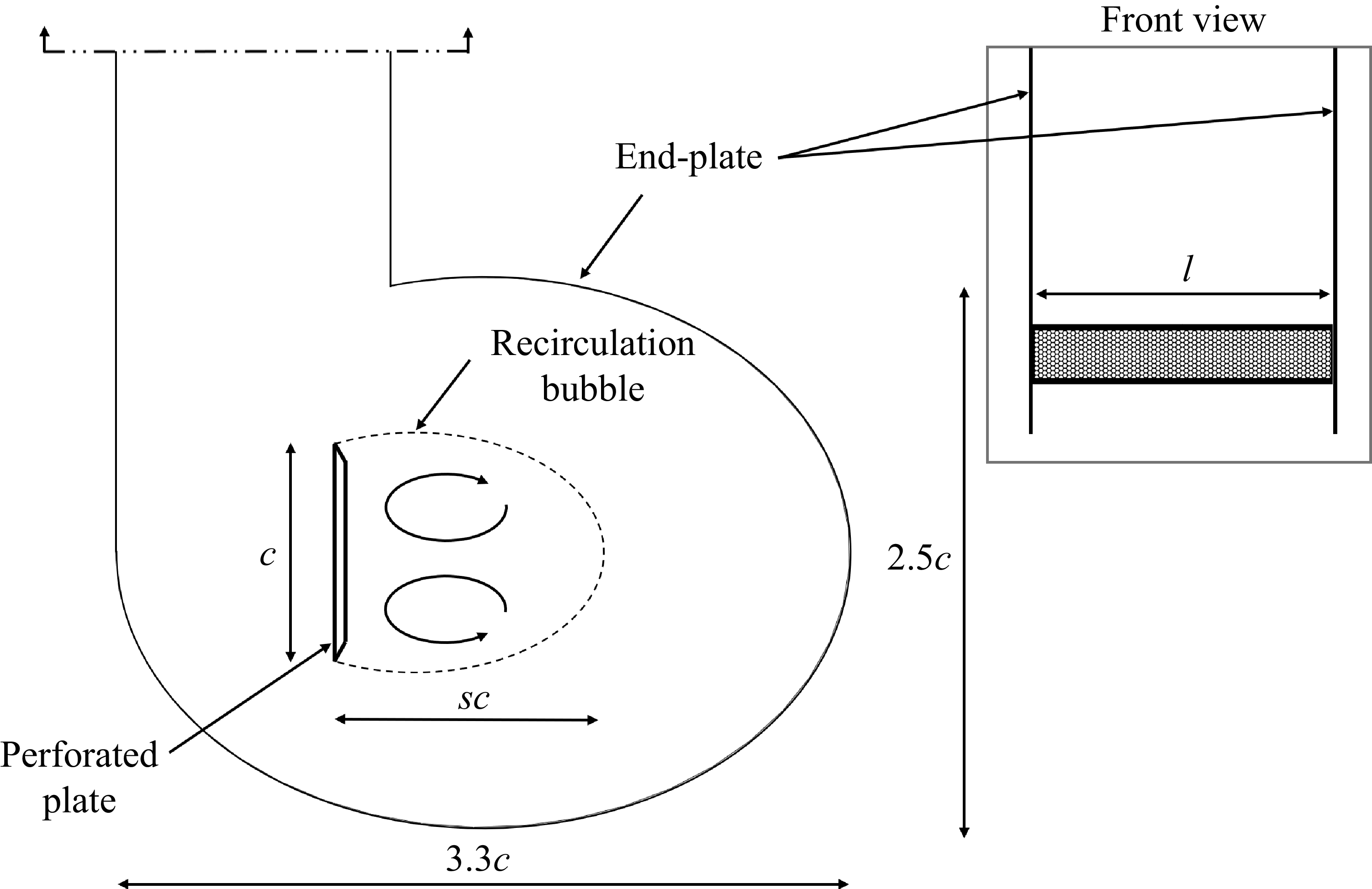
 s
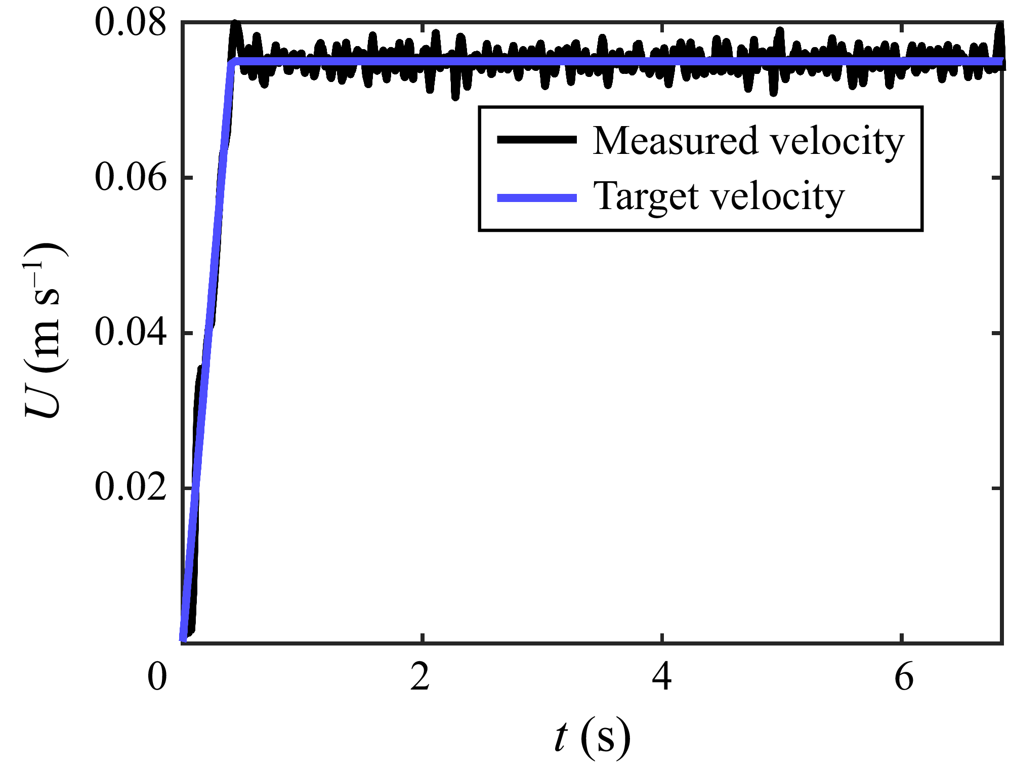
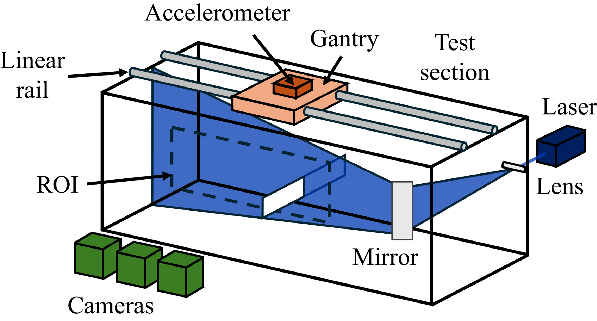

 cd
 T
 β
 T⩽0.5
 β=50.5%
 cd∈[0.7,1.9]
 T∈[7,8]
 6×10³
 9×10⁴

 T=0.25
 T=1
 T=4
 β=0%
 β=24%
 β=50.5%
 ×
 +

 T=8
 β=0%,24%,50.5%
 ×
 +

 s
 T
 s(T)
 β={0%,12%,16%,28%}

 T
 a(β)=2.63−4.29β
 Tb(β)
 b(β)=0.529+0.740β
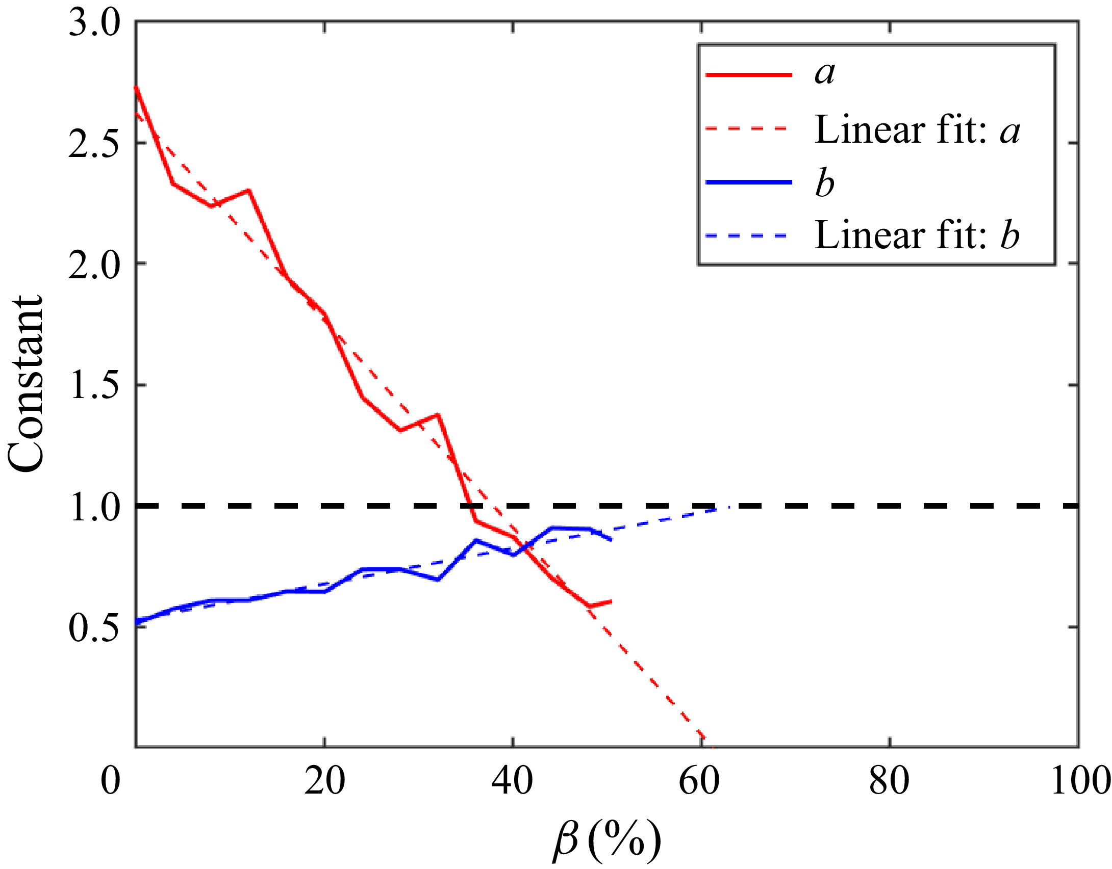
 T∈[0.4,4]
 β

 T
 T=0.25

 α(β)
 +
 β≠0
 β=0
 β≠0
 β=0

 β={0%,24%,50.5%}
 β=50.5%

 T
 β∈{0%,24%,50.5%}
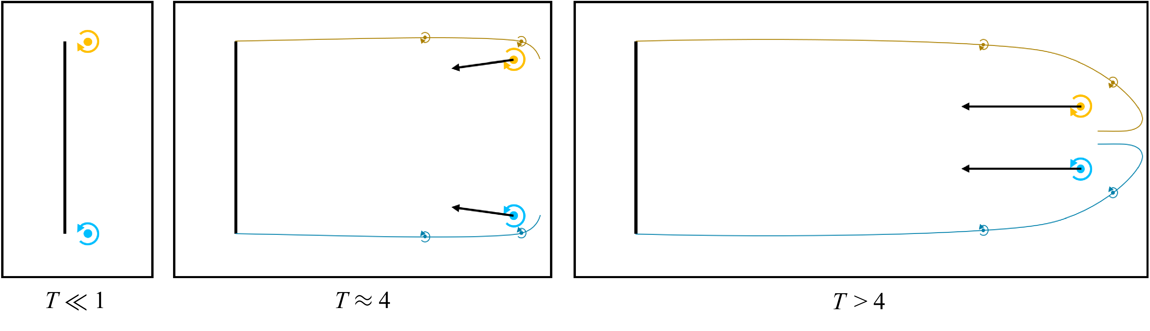
 β=50.5%



