1 Introduction
Detailed understanding of the interplay between colloidal-scale forces in suspensions, and how their relative strengths change with flow, is an important element in forming structure–property relationships required for predictive theory and materials design, for both steady-state and transient flow conditions. Sustained, flow-dependent microstructural asymmetry underlies non-Newtonian steady-state rheology in Brownian suspensions, and can be traced to the duration and trajectories of pair-level particle encounters, which are in turn shaped by the relative dominance of hydrodynamic and non-hydrodynamic microscopic forces. Each of these forces produces colloidal motion over a distinct time scale: if the speed of Brownian motion is high compared to advection (or particles are rough), a relative Stokes flow trajectory will be overlaid with many random displacements before the encounter is complete. On average, this leads to asymmetric distortion of the suspension microstructure. A continuous competition between building and relaxing structure thus sustains non-Newtonian rheology. An understanding of the time scales over which various microscopic forces – hydrodynamic, Brownian and interparticle – distort and relax structure, and thus develop and sustain non-Newtonian rheology, is important in particle formulations to give desired material responsiveness. It is also of broader heuristic value, e.g. in understanding how biological systems change surface properties to modulate the media in which they operate. While much robust theory exists for steady-state flow, far less study has been devoted to the study of transient rheology and is relevant to intermittent flow ranging from shaving cream dispersions to migration of nuclei during biological cell division.
The evolution of a colloidal structure from equilibrium to non-equilibrium configuration under an applied external flow occurs over a finite time; this time scale is set by microscopic transport processes – hydrodynamic, entropic and interparticle – that shape structural arrangement. Our recent work (Mohanty & Zia Reference Mohanty and Zia2018) showed that a suspension driven at a rate that produces shear thickening may at first ‘time thin’ – meaning that increasing flow strength may lead to short-time shear thinning, followed by steady-state flow thickening, owing to the balance between advective and Brownian displacements. Similarly, the relaxation of a deformed colloidal microstructure after external flow is removed is set by time scales over which microscopic processes smooth density and stress gradients; in purely repulsive systems, Brownian motion is the only driving force for relaxation. But other microscopic forces besides the Brownian force can enhance or hinder relaxation. In particular, the non-equilibrium hydrodynamic and entropic contributions to non-Newtonian rheology are not easily decoupled during startup flow, because both these contributions coevolve throughout the transient and long-time steady flow (Mohanty & Zia Reference Mohanty and Zia2018). In contrast, flow cessation immediately ‘strips off’ direct, flow-induced hydrodynamic contributions to particle motion and rheology, leaving only contributions that are coupled to entropic forces. When the externally imposed field or force driving suspension flow is suddenly removed, induced fluid motion can actually continue for a period of time as the microstructure relaxes and entrains fluid. The flow induced by thermodynamic forces persists until the colloidal microstructure recovers its equilibrium configuration (Mackay & Kaffashi Reference Mackay and Kaffashi1995; Zia & Brady Reference Zia and Brady2013).
Experimental studies of rheology after sudden flow cessation have confirmed the existence of at least two time scales: the instantaneous relaxation of direct, flow-induced stress, and other relaxation. In studies of the behaviour of sheared hard-particle suspensions, Mackay & Kaffashi (Reference Mackay and Kaffashi1995) found that the contribution to stress arising directly from the external flow (the so-called hydrodynamic stress) dissipates instantaneously upon flow cessation. However, the remaining stress continued to decay over time, which was attributed to the presence of entropic stress associated with relaxing particle microstructure. To quantify the rate of such relaxation, Kaffashi et al. (Reference Kaffashi, O’Brien, Mackay and Underwood1997) measured the rate of long-time relaxation of the elastic stress (the total stress minus the hydrodynamic stress). They found power-law relaxation and proposed that the exponent depends on the pre-cessation shear rate. Taking this idea further, Watanabe et al. (Reference Watanabe, Yao, Yamagishi, Osaki, Shitata, Niwa and Morishima1996) identified that the dependence of relaxation rate on pre-cessation shear rate is most pronounced in the shear-thickening regime, i.e. strong flow, and vanishes in the shear-thinning regime (weak flow). They hypothesized a microstructural mechanism for this behaviour: formation of hydroclusters and structural asymmetry, which become more pronounced with strong flow and thus result in a faster relaxation. However, no images or measurements of post-cessation structural evolution were available to support this hypothesis. Complementary theoretical studies could provide insight into some of these questions and guide particle formulation to suppress (or promote) such structure. However, relatively few such studies have been carried out to connect rheology with the colloidal microstructure.
To study the relationship between post-cessation stress decay and microstructural relaxation, Foss (Reference Foss1999), Zia & Brady (Reference Zia and Brady2013) and more recently Marenne et al. (Reference Marenne, Morris, Foss and Brady2017) studied sheared colloidal dispersions utilizing Brownian dynamics and Stokesian dynamics simulations. All found an initially rapid decay of entropic stress arising from boundary-layer relaxation, followed at long times by long-range structural relaxation and stress decay. All three studies ascribed the rate of relaxation to the thickness of the boundary layer, which scales inversely with the strength of the external flow, giving a connection between compressed structure, flow strength and speed of relaxation. Together, these studies focused on two asymptotic limits: freely draining colloids; and smooth, hydrodynamically interacting colloids. But the transition from one limit to the other remained unexplored. In addition, no prior study examines the decoupling of induced hydrodynamic tractions from Brownian motion that underlie Brownian drift. Active microrheology provides an ideal framework for decoupling these contributions. Passive microrheology has long been utilized to interrogate complex fluids such as cells (Guilford, Lantz & Gore Reference Guilford, Lantz and Gore1995; Bausch et al. Reference Bausch, Ziemann, Boulbitch, Jacobson and Sackmann1998; Lau et al. Reference Lau, Hoffman, Davies, Crocker and Lubensky2003), actin networks (Ziemann, Radler & Sackmann Reference Ziemann, Radler and Sackmann1994; Gisler & Weitz Reference Gisler and Weitz1998), gelatin (Freundlich & Sfifriz Reference Freundlich and Sfifriz1923), DNA and polyethylene oxide solutions (Mason et al. Reference Mason, Genevan, van Zanten, Wirtz and Kuo1997; Gomez-Solano & Bechinger Reference Gomez-Solano and Bechinger2015), the glass transition in colloids (Habdas et al. Reference Habdas, Schaar, Levitt and Weeks2004), as well as fundamental interactions between pairs of colloidal spheres (Crocker Reference Crocker1997; Crocker et al. Reference Crocker, Valentine, Weeks, Gisler, Kaplan, Yodh and Weitz2000; Levine & Lubensky Reference Levine and Lubensky2000; Wulfert, Seifert & Speck Reference Wulfert, Seifert and Speck2017; Dolata & Zia Reference Dolata and Zia2018) and entropic forces in binary colloids (Crocker et al. Reference Crocker, Matteo, Dinsmore and Yodh1999).
Microrheological experimental studies, theoretical models and dynamic simulations have recovered steady-state non-Newtonian behaviours, including force thinning and thickening, flow-induced diffusion, normal stress differences and response to oscillatory flows (Habdas et al. Reference Habdas, Schaar, Levitt and Weeks2004; Carpen & Brady Reference Carpen and Brady2005; Furst Reference Furst2005; Squires & Brady Reference Squires and Brady2005; Khair & Brady Reference Khair and Brady2005, Reference Khair and Brady2006, Reference Khair and Brady2007, Reference Khair and Brady2008; Squires Reference Squires2008; Gazuz et al. Reference Gazuz, Puertas, Voigtmann and Fuchs2009; Sriram et al. Reference Sriram, DePuit, Squires and Furst2009; Wilson et al. Reference Wilson, Harrison, Schfield, Arlt and Poon2009; Squires & Mason Reference Squires and Mason2010; Zia & Brady Reference Zia and Brady2010; Gnann et al. Reference Gnann, Gazuz, Puertas, Fuchs and Voigtmann2011; Schultz & Furst Reference Schultz and Furst2011; DePuit & Squires Reference DePuit and Squires2012; Zia & Brady Reference Zia and Brady2012, Reference Zia and Brady2013; Swan & Zia Reference Swan and Zia2013; Voigtmann & Fuchs Reference Voigtmann and Fuchs2013; Swan, Zia & Brady Reference Swan, Zia and Brady2014; Chu & Zia Reference Chu and Zia2016, Reference Chu and Zia2017; Hoh & Zia Reference Hoh and Zia2016a,Reference Hoh and Ziab; Nazockdast & Morris Reference Nazockdast and Morris2016; Leitmann et al. Reference Leitmann, Mandal, Fuchs, Puertas and Franosch2018). But, in both theory and experiment, the majority of the focus thus far has remained on steady-state response of the material, with comparatively little focus devoted to temporal evolution. Recent theoretical studies of active microrheology reveal direct connections between entropic and hydrodynamic forces that produce generalized Stokes–Einstein relations and find connections between fluctuation and dissipation that cannot be obtained via shear rheology (Zia Reference Zia2018; Chu & Zia Reference Chu and Zia2019). A detailed review of theoretical active microrheology can be found in Zia (Reference Zia2018).
Zia & Brady (Reference Zia and Brady2013) investigated nonlinear transient microrheology during flow startup and cessation in freely draining colloidal dispersions with a theoretical model for semidilute suspensions, and Brownian dynamics simulations for concentrated suspensions. As noted above, they found at least two relaxation modes: an early-time fast relaxation, where the majority of the entropic stress dissipates by relaxation of the boundary layer, followed by slower long-time relaxation as the wake fills in. The same scaling as found for shear rheology (Foss Reference Foss1999) was recovered, thus showing that microrheology recovers the important qualitative behaviour of transient shear rheology. Zia & Brady (Reference Zia and Brady2013) also found that the probe travels backwards through the suspension upon removal of the external force, and they connected this deterministic motion to the entropic energy stored in the distorted configuration. This ‘entropic recovery’ formed a connection between stress and entropically stored energy. Later, Gomez-Solano & Bechinger (Reference Gomez-Solano and Bechinger2015) performed microrheological flow cessation experiments in viscoelastic fluids, and confirmed the same motion of the probe recoil after sudden removal of the external force. They also concluded that the relaxation behaviours after flow cessation represent the mechanisms by which stored energy in the microstructure gets dissipated back to the fluid, thereby recovering the theoretical results of Zia & Brady (Reference Zia and Brady2013). However, neither study addressed the role of hydrodynamic interactions. Our recent work incorporated hydrodynamics into a model of startup flow in microrheology (Mohanty & Zia Reference Mohanty and Zia2018). We found that hydrodynamic interactions influence structural and rheological evolution during flow startup where stronger hydrodynamic coupling between particles slows both structural and rheological evolution during flow startup.
The aim of this study is to explore the impact of hydrodynamic interactions and entropic forces on the relaxation of the structure and rheology upon microrheological flow cessation in suspensions of hydrodynamically interacting colloids. To do so, we employ an excluded-annulus model (Russel Reference Russel1984), which gives an idealized means to systematically vary the strength of hydrodynamic interactions between particles by tuning the range of spherically symmetric interparticle repulsion. We formulate and solve a transient Smoluchowski equation that governs the particle arrangement around a probe particle. We find that the structure relaxes faster with increasing pre-cessation flow strength, but takes longer with increasing strength of hydrodynamic interactions. Utilizing statistical mechanics, we connect the transient structure with probe motion and rheology, finding that the early-time viscosity decay is set by the relaxation of the particle-rich boundary layer near the probe surface. Hydrodynamic interactions slow this process because they hinder relative motion between particles. At long times, the relaxation behaviour becomes independent of the pre-cessation flow strength as the microstructure loses its memory. We find that the structural distortion can do useful work: the thermodynamic force during relaxation ejects the probe in the direction opposite to the pre-cessation external force. Stronger hydrodynamic coupling slows this ejection. We show that the probe back-travel provides a means to measure average flow energy density stored in the deformed structure.
The remainder of the paper is organized as follows. The model system is introduced and the theoretical framework is developed in § 2. The time-dependent Smoluchowski equation that governs the spatiotemporal evolution of the particle arrangement around the probe particle is derived in § 2.2, and the time-dependent structural evolution is connected to the probe motion and the transient viscosity in § 2.3. Results are presented in § 3, starting with asymptotic analysis of weak and strong hydrodynamic interactions limit, followed by relaxation of the structure and probe motion for arbitrary strengths of hydrodynamics. Results are obtained for arbitrary strengths of pre-cessation external force on the probe. Next, the probe back-travel is connected to the steady-state non-equilibrium osmotic pressure associated with the deformed structure. The study is concluded with a discussion in § 4.
2 Theoretical framework
The microrheology model system comprises an assembly of  $N$ neutrally buoyant Brownian spheres of size
 $a$ homogeneously dispersed in a Newtonian solvent of density
 $\unicode[STIX]{x1D70C}$ and viscosity
 $\unicode[STIX]{x1D702}_{s}$. One particle, the probe, is driven by an external force,
 $\boldsymbol{F}^{ext}$, while the remaining
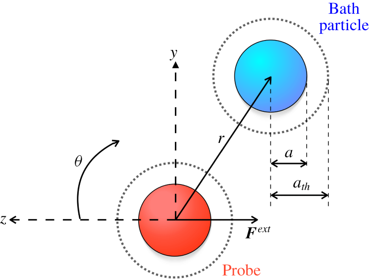
 $N-1$ surrounding bath particles remain force- and torque-free (figure 1). Movement of the probe sets the fluid and particles into motion. The Reynolds number,
 $Re=\unicode[STIX]{x1D70C}Ua/\unicode[STIX]{x1D702}_{s}$, describing the inertia of the fluid flow relative to the viscous forces, is small because the particles are small. Here,
 $U$ is the characteristic velocity of the probe. Stokes’ equations thus govern the motion of the fluid. As the probe begins to move through the suspension, it interacts with the surrounding bath particles and alters their arrangement around the probe (the microstructure), which in turn changes probe motion and the rheological properties of the suspension. Following initial application of the force, it takes time for the probe to encounter all permissible microstructures on its way through the bath. Mohanty & Zia (Reference Mohanty and Zia2018) showed that, once the probe successfully resolves pair encounters with many such configurations, average probe speed, and hence viscosity, reach steady state. In this work, we study the opposite transient problem: time-dependent probe motion after the external force is removed. At each moment in time, the probe samples one of the many permissible bath particle configurations. These are described by a spatiotemporal evolution of the probability distribution of the bath particles around the probe, presented in § 2.2. We utilize the temporally evolving microstructure to formulate a time-dependent ensemble-average probe velocity and the time-dependent viscosity of the surrounding medium in § 2.3.
Model system.

2.1 Repulsive forces and hydrodynamic interactions
In Stokes flow, the relative motion of perfectly smooth non-colloidal spheres is fore–aft symmetric and, in the case of externally forced particles, the entrainment of one particle by another decays linearly as the inverse of the distance between the two. However, repulsive forces, such as surface asperities or surface treatments aimed at steric stabilization, destroy Stokes flow symmetry and also quantitatively weaken hydrodynamic interactions by keeping particles well separated. Thus, a particle will have a hydrodynamic radius,  $a$, where the no-slip condition is obeyed, and may also have a thermodynamic radius,
 $a_{th}$, where a no-flux condition is enforced at contact. The two may coincide or
 $a_{th}$ may extend well beyond the no-slip surface, which can be represented by the excluded-annulus (shell) model (Russel Reference Russel1984) as illustrated in figure 1. This is a simplified model for a repulsive potential. The minimum approach distance between the particles,
 $r_{min}$, is set by the thermodynamic radius and signifies the radial separation distance at which thermodynamic surfaces come into contact with each other. For a monodisperse suspension of hard spheres,
 $r_{min}=2a_{th}$. The strength of hydrodynamic coupling weakens as the minimum approach distance between two particles grows. If the surface treatment can be modelled as a spherically symmetric potential, the excluded-shell model (Russel Reference Russel1984) provides a simple yet effective means by which to systematically tune the strength of hydrodynamic interactions, by varying the minimum approach distance, as shown in figure 1. The excluded-shell thickness, scaled on the hydrodynamic size, defines a dimensionless repulsion range,
 $\unicode[STIX]{x1D705}\equiv (a_{th}-a)/a$. It is convenient to express the closest separation as
 $r_{min}=2a(1+\unicode[STIX]{x1D705})$. When the thermodynamic size of the particles is much larger than the hydrodynamic radius,
 $\unicode[STIX]{x1D705}\rightarrow \infty$, the interparticle repulsion is long-ranged and hydrodynamic disturbance flows decay to negligibly weak before reaching another particle. In the opposite limit,
 $\unicode[STIX]{x1D705}\rightarrow 0$, particles can come close enough to experience strong lubrication forces. In the intermediate regime,
 $\unicode[STIX]{x1D705}\sim O(1)$, the particles experience hydrodynamic interactions at all separations.
The hard-sphere potential prevents any overlap of the thermodynamic surfaces, and is zero away from contact:
 $$\begin{eqnarray}V(r)=\left\{\begin{array}{@{}ll@{}}\infty ,\quad & \text{if }r\leqslant 2a_{th},\\ 0,\quad & \text{if }r>2a_{th}.\end{array}\right.\end{eqnarray}$$
The hard-sphere potential represents the excluded-shell model (Russel Reference Russel1984) where the particles do not interact beyond their minimum approach distance,  $r_{min}=2a_{th}$, and an infinite force at contact prevents particle overlap. Other interparticle forces arising from a spherically symmetric potential can be easily incorporated into this model. The volume fraction in a suspension is defined on the thermodynamic size of the particles; in a monodisperse suspension,
 $\unicode[STIX]{x1D719}=4\unicode[STIX]{x03C0}a_{th}^{3}n/3$, where
 $n$ is the number density of particles.
2.2 Evolving microstructure
Here we derive expressions governing the spatiotemporal evolution of the particle microstructure, restricting our attention to the semidilute regime where the volume fraction of particles is small and only pair interactions are important. At higher concentrations, three-body and higher-order interactions become important, for which detailed modelling typically requires computational approaches. Because the frame of reference is centred on the probe, its pair-level interactions with the bath are  $O(1)\times O(\unicode[STIX]{x1D719})=O(\unicode[STIX]{x1D719})$. In practice, such a model is valid up to approximately 15 % volume fraction (de Kruif et al. Reference de Kruif, van Lersel, Vrij and Russel1985; Bedeaux Reference Bedeaux1987; van der Werff et al. Reference van der Werff, de Kruif, Blom and Mellema1989; Shikata & Pearson Reference Shikata and Pearson1994). Pair-level interactions underlie many important non-Newtonian phenomenon, such as hydrodynamic diffusion (Davis & Hill Reference Davis and Hill1992), polydisperse sedimentation (Batchelor Reference Batchelor1982), high-frequency linear viscoelasticity (Lionberger & Russel Reference Lionberger and Russel1994), shear thinning (Batchelor Reference Batchelor1976; Bergenholtz, Brady & Vicic Reference Bergenholtz, Brady and Vicic2002) and shear thickening (Brady & Bossis Reference Brady and Bossis1985; Barnes Reference Barnes1989; D’Haene, Mewis & Fuller Reference D’Haene, Mewis and Fuller1993; Bender & Wagner Reference Bender and Wagner1995; Bergenholtz et al. Reference Bergenholtz, Brady and Vicic2002; Maranzano & Wagner Reference Maranzano and Wagner2002). Microrheology theory for dilute suspensions has been tested and validated in the experimental literature, including cells (Guilford et al. Reference Guilford, Lantz and Gore1995; Bausch et al. Reference Bausch, Ziemann, Boulbitch, Jacobson and Sackmann1998; Lau et al. Reference Lau, Hoffman, Davies, Crocker and Lubensky2003), actin networks (Ziemann et al. Reference Ziemann, Radler and Sackmann1994; Gisler & Weitz Reference Gisler and Weitz1999), gelatin (Freundlich & Sfifriz Reference Freundlich and Sfifriz1923), DNA and polyethylene oxide solutions (Mason et al. Reference Mason, Genevan, van Zanten, Wirtz and Kuo1997), wormlike micelles and polymer solutions (Gomez-Solano & Bechinger Reference Gomez-Solano and Bechinger2015), non-equilibrium behaviours in colloids (Sriram, Meyer & Furst Reference Sriram, Meyer and Furst2010), the behaviour of colloids near glass transition (Habdas et al. Reference Habdas, Schaar, Levitt and Weeks2004), fundamental interactions between pairs of colloids (Crocker Reference Crocker1997; Crocker et al. Reference Crocker, Valentine, Weeks, Gisler, Kaplan, Yodh and Weitz2000; Levine & Lubensky Reference Levine and Lubensky2000) and entropic forces in binary colloids (Crocker et al. Reference Crocker, Matteo, Dinsmore and Yodh1999).
Pair-level configurations are described by the pair probability density,  $P_{2}(\boldsymbol{x}_{1},\boldsymbol{x}_{2},t)$, the probability of finding the probe (particle 1) at a position
 $\boldsymbol{x}_{1}$, and a bath particle (particle 2) at
 $\boldsymbol{x}_{2}$ at time
 $t$. The pair-level generalized Smoluchowski equation governs its evolution:
 $$\begin{eqnarray}\frac{\unicode[STIX]{x2202}P_{2}}{\unicode[STIX]{x2202}t}+\unicode[STIX]{x1D735}_{1}\boldsymbol{\cdot }\boldsymbol{j}_{1}+\unicode[STIX]{x1D735}_{2}\boldsymbol{\cdot }\boldsymbol{j}_{2}=0.\end{eqnarray}$$
Here  $\boldsymbol{j}_{1}$ and
 $\boldsymbol{j}_{2}$ are the configuration-dependent flux of the probe and bath particles, respectively, arising from the external force on the probe, Brownian forces and interparticle forces
 $\boldsymbol{F}_{\unicode[STIX]{x1D6FC}}^{P}=-\unicode[STIX]{x1D735}_{\unicode[STIX]{x1D6FC}}V$, where
 $V$ denotes the interparticle potential and the gradient is taken with respect to the position of particle
 $\unicode[STIX]{x1D6FC}$:
 $$\begin{eqnarray}\left.\begin{array}{@{}c@{}}\displaystyle \boldsymbol{j}_{1}=\boldsymbol{U}_{1}P_{2}(\boldsymbol{x}_{1},\boldsymbol{x}_{2})=[\unicode[STIX]{x1D648}_{11}\boldsymbol{\cdot }\boldsymbol{F}_{1}^{ext}-(\unicode[STIX]{x1D63F}_{11}\boldsymbol{\cdot }\unicode[STIX]{x1D735}_{1}+\unicode[STIX]{x1D63F}_{12}\boldsymbol{\cdot }\unicode[STIX]{x1D735}_{2})-(\unicode[STIX]{x1D63F}_{11}\boldsymbol{\cdot }\unicode[STIX]{x1D735}_{1}V+\unicode[STIX]{x1D63F}_{12}\boldsymbol{\cdot }\unicode[STIX]{x1D735}_{2}V)]P_{2},\\ \displaystyle \boldsymbol{j}_{2}=\boldsymbol{U}_{2}P_{2}(\boldsymbol{x}_{1},\boldsymbol{x}_{2})=[\unicode[STIX]{x1D648}_{21}\boldsymbol{\cdot }\boldsymbol{F}_{1}^{ext}-(\unicode[STIX]{x1D63F}_{21}\boldsymbol{\cdot }\unicode[STIX]{x1D735}_{1}+\unicode[STIX]{x1D63F}_{22}\boldsymbol{\cdot }\unicode[STIX]{x1D735}_{2})-(\unicode[STIX]{x1D63F}_{21}\boldsymbol{\cdot }\unicode[STIX]{x1D735}_{1}V+\unicode[STIX]{x1D63F}_{22}\boldsymbol{\cdot }\unicode[STIX]{x1D735}_{2}V)]P_{2}.\end{array}\right\}\end{eqnarray}$$
Here,  $\unicode[STIX]{x1D648}_{\unicode[STIX]{x1D6FC}\unicode[STIX]{x1D6FD}}$ is the configuration-dependent hydrodynamic mobility tensor that transmits hydrodynamic tractions on the surface of particle
 $\unicode[STIX]{x1D6FD}$ to the motion of particle
 $\unicode[STIX]{x1D6FC}$. It is related to the diffusion tensor,
 $\unicode[STIX]{x1D63F}_{\unicode[STIX]{x1D6FC}\unicode[STIX]{x1D6FD}}$, as
 $\unicode[STIX]{x1D63F}_{\unicode[STIX]{x1D6FC}\unicode[STIX]{x1D6FD}}=kT\unicode[STIX]{x1D648}_{\unicode[STIX]{x1D6FC}\unicode[STIX]{x1D6FD}}$. In the microrheology framework,
 $\unicode[STIX]{x1D6FC},\unicode[STIX]{x1D6FD}\in \{1,2\}$. The mobility tensor depends on particle configuration parameters, viz. particle shape, size and interparticle separation,
 $r=|\boldsymbol{r}|$, and also depends on the range of interparticle repulsion,
 $\unicode[STIX]{x1D705}$. To obtain the motion along and transverse to the line of centres
 $\hat{\boldsymbol{r}}=\boldsymbol{r}/r$ between an interacting pair, the mobility tensor can be projected through the orthogonal bases
 $\hat{\boldsymbol{r}}\hat{\boldsymbol{r}}$ and
 $\unicode[STIX]{x1D644}-\hat{\boldsymbol{r}}\hat{\boldsymbol{r}}$, respectively:
 $$\begin{eqnarray}\unicode[STIX]{x1D648}_{\unicode[STIX]{x1D6FC}\unicode[STIX]{x1D6FD}}^{UF}=\frac{1}{6\unicode[STIX]{x03C0}\unicode[STIX]{x1D702}_{s}a}\{x_{\unicode[STIX]{x1D6FC}\unicode[STIX]{x1D6FD}}^{a}(r/a)\hat{\boldsymbol{r}}\hat{\boldsymbol{r}}+y_{\unicode[STIX]{x1D6FC}\unicode[STIX]{x1D6FD}}^{a}(r/a)(\unicode[STIX]{x1D644}-\hat{\boldsymbol{r}}\hat{\boldsymbol{r}})\},\end{eqnarray}$$
where  $\unicode[STIX]{x1D644}$ is the identity tensor. The coefficients
 $x_{\unicode[STIX]{x1D6FC}\unicode[STIX]{x1D6FD}}^{a}$ and
 $y_{\unicode[STIX]{x1D6FC}\unicode[STIX]{x1D6FD}}^{a}$ give the strength of the longitudinal and transverse coupling between a pair, and are functions only of particle shape, size ratio and relative separation (Jeffrey & Onishi Reference Jeffrey and Onishi1984; Kim & Karilla Reference Kim and Karilla1991). For same-size spheres, only their separation matters. The range of permissible relative separations,
 $r/a$, is set by
 $\unicode[STIX]{x1D705}$, which we systematically vary to study the influence of hydrodynamic interactions.
We adopt a frame of reference moving with the probe centred at  $\boldsymbol{z}=\boldsymbol{x}_{1}$, and a bath particle at
 $\boldsymbol{r}=\boldsymbol{x}_{2}-\boldsymbol{x}_{1}$. The probability density describing all permissible arrangements of the probe and a bath particle can then be related to the pair-distribution function,
 $g(\boldsymbol{r},t)$, as
 $$\begin{eqnarray}P_{2}(\boldsymbol{x}_{1},\boldsymbol{x}_{2})=P_{2}(\boldsymbol{z},\boldsymbol{r})=P_{1/1}(\boldsymbol{r},t\mid \boldsymbol{z})P_{1}(\boldsymbol{z})=ng(\boldsymbol{r},t)P_{1}(\boldsymbol{z}),\end{eqnarray}$$
where  $n$ is the number density of surrounding bath particles. We insert equations (2.3) and (2.5) into equation (2.2), and integrate over all positions of the probe,
 $\boldsymbol{z}$, to obtain the equation governing structural evolution of a bath particle:
 $$\begin{eqnarray}\frac{\unicode[STIX]{x2202}g}{\unicode[STIX]{x2202}t}=\unicode[STIX]{x1D735}\boldsymbol{\cdot }(\unicode[STIX]{x1D63F}_{r}\boldsymbol{\cdot }\unicode[STIX]{x1D735}g+\unicode[STIX]{x1D63F}_{r}\boldsymbol{\cdot }\unicode[STIX]{x1D735}Vg-\unicode[STIX]{x1D648}_{r}\boldsymbol{\cdot }\boldsymbol{F}^{ext}g),\end{eqnarray}$$
where the gradient is taken with respect to the position of the bath particle,  $\boldsymbol{r}$. The relative hydrodynamic mobility
 $\unicode[STIX]{x1D648}_{21}-\unicode[STIX]{x1D648}_{11}$ has been written compactly as
 $\unicode[STIX]{x1D648}_{r}$, and the relative Brownian diffusivity
 $\unicode[STIX]{x1D63F}_{11}-\unicode[STIX]{x1D63F}_{12}-\unicode[STIX]{x1D63F}_{21}+\unicode[STIX]{x1D63F}_{22}$ as
 $\unicode[STIX]{x1D63F}_{r}$, following the approach of Batchelor (Reference Batchelor1976). For simplicity, we take the probe and bath particle to have the same size, giving
 $\unicode[STIX]{x1D648}_{11}=\unicode[STIX]{x1D648}_{22}$ and
 $\unicode[STIX]{x1D648}_{12}=\unicode[STIX]{x1D648}_{21}$. The relative mobility can thence be written in terms of the relative diffusivity tensor as
 $(\unicode[STIX]{x1D648}_{21}-\unicode[STIX]{x1D648}_{11})=-\unicode[STIX]{x1D63F}_{r}/2kT$. The relative Brownian diffusivity tensor is projected through the orthogonal bases
 $\hat{\boldsymbol{r}}\hat{\boldsymbol{r}}$ and
 $(\unicode[STIX]{x1D644}-\hat{\boldsymbol{r}}\hat{\boldsymbol{r}})$ to obtain the relative motion along and transverse to the line of centres of an interacting pair:
 $$\begin{eqnarray}6\unicode[STIX]{x03C0}\unicode[STIX]{x1D702}_{s}a\unicode[STIX]{x1D63F}_{r}=2kT[G(r/a)\hat{\boldsymbol{r}}\hat{\boldsymbol{r}}+H(r/a)(\unicode[STIX]{x1D644}-\hat{\boldsymbol{r}}\hat{\boldsymbol{r}})].\end{eqnarray}$$
The scalar hydrodynamic functions  $G=x_{11}^{a}-x_{12}^{a}$ and
 $H=y_{11}^{a}-y_{12}^{a}$ give the relative mobility: how easy it is for a bath particle to approach the probe moving along
 $(G)$ or transverse to
 $(H)$ their line of centres. These, of course, vary with
 $\unicode[STIX]{x1D705}$; for
 $\unicode[STIX]{x1D705}\neq 0$, two regions develop upstream: a zone of ‘filtered’ trajectories around the line of centres that allow direct contact, and exterior to that envelope, trajectories are deflected by hydrodynamic interactions (see figure 5 in Hoh & Zia (Reference Hoh and Zia2015)). As
 $\unicode[STIX]{x1D705}\rightarrow \infty$, the envelope becomes so large that no trajectories are deflected and all particles approaching within
 $r_{min}$ make direct contact; this is the freely draining limit. In the opposite limit,
 $\unicode[STIX]{x1D705}=0$, the structure is spherically symmetric. We will systematically examine many values of
 $\unicode[STIX]{x1D705}$ between these two limits.
Equation (2.1) specifies no relative particle flux at contact and there is no long-range order, providing two boundary conditions: the equation governing the transient microstructural evolution for startup flow was derived by Mohanty & Zia (Reference Mohanty and Zia2018),
 $$\begin{eqnarray}\unicode[STIX]{x1D735}\boldsymbol{\cdot }[\unicode[STIX]{x1D63F}_{r}\boldsymbol{\cdot }\unicode[STIX]{x1D735}g-Pe\boldsymbol{U}_{r}g{\mathcal{H}}(t)]=\frac{\unicode[STIX]{x2202}g}{\unicode[STIX]{x2202}t},\end{eqnarray}$$
where all quantities have been made dimensionless as
 $$\begin{eqnarray}r\sim a_{th},\quad \unicode[STIX]{x1D63F}_{r}\sim 2D_{0},\quad \boldsymbol{U}_{r}\sim U_{0}\quad \text{and}\quad t\sim a_{th}^{2}/2D_{0},\end{eqnarray}$$
and the Péclet number setting the strength of external flow to diffusion,  $Pe=F^{ext}/(2kT/a_{th})$, arises naturally from the scaling. The velocity of the bath particle relative to the probe,
 $\boldsymbol{U}_{r}=(\unicode[STIX]{x1D648}_{21}-\unicode[STIX]{x1D648}_{11})\boldsymbol{\cdot }\boldsymbol{F}^{ext}$, arises instantly upon application of the external force as indicated by the Heaviside function,
 ${\mathcal{H}}(t)$. As
 $t\rightarrow \infty$ after startup, the microstructure reaches its steady-state configuration,
 $g^{SS}(\boldsymbol{r};Pe,\unicode[STIX]{x1D705})$, set by flow strength
 $Pe$ and strength of hydrodynamic interactions,
 $\unicode[STIX]{x1D705}$. Upon removal of the external force,
 $\boldsymbol{U}_{r}$ vanishes instantly, giving the equations governing the post-cessation relaxation:
 $$\begin{eqnarray}\displaystyle & \displaystyle \unicode[STIX]{x1D735}\boldsymbol{\cdot }(\unicode[STIX]{x1D63F}_{r}\boldsymbol{\cdot }\unicode[STIX]{x1D735}g)=\frac{\unicode[STIX]{x2202}g}{\unicode[STIX]{x2202}t}, & \displaystyle\end{eqnarray}$$
 $$\begin{eqnarray}\displaystyle & \displaystyle \hat{\boldsymbol{r}}\boldsymbol{\cdot }(\unicode[STIX]{x1D63F}_{r}\boldsymbol{\cdot }\unicode[STIX]{x1D735}g)=0\quad \text{at }r=2, & \displaystyle\end{eqnarray}$$
 $$\begin{eqnarray}\displaystyle & \displaystyle g\sim 1\quad \text{as }r\rightarrow \infty , & \displaystyle\end{eqnarray}$$
 $$\begin{eqnarray}\displaystyle & \displaystyle g(\boldsymbol{r},t;Pe,\unicode[STIX]{x1D705})=g^{SS}(\boldsymbol{r};Pe,\unicode[STIX]{x1D705})\quad \text{at }t=0, & \displaystyle\end{eqnarray}$$
 $g^{SS}(\boldsymbol{r};Pe,\unicode[STIX]{x1D705})$, is now the initial condition. The gradients in the microstructure drive its relaxation via Brownian diffusion only. Equations (2.10) thus govern structural relaxation for any value of
 $Pe$ or
 $\unicode[STIX]{x1D705}$ prior to flow cessation.
2.3 Transient viscosity
We examine the evolution of the viscosity following removal of the external force driving the probe. We assume that the suspension has been flowing for a long time at steady state prior to this. Upon force shutoff, the probe will continue to travel, but now backwards (there is no inertia, so there will be no further forward excursion). As it does so, it will explore many relaxing configurations. Repeated realizations of this scenario enable the probe to sample many permissible configurations at each post-shutoff time to give a time-dependent suspension average probe velocity,  $\langle \boldsymbol{U}_{1}\rangle (t)$. The angle brackets indicate an average over surrounding bath configurations at a time
 $t$, and this mean probe motion relaxes over time. Insertion of this velocity into Stokes’ drag law (Squires & Brady Reference Squires and Brady2005; Khair & Brady Reference Khair and Brady2006),
 $\boldsymbol{F}^{ext}=6\unicode[STIX]{x03C0}\unicode[STIX]{x1D702}^{eff}(t)a\langle \boldsymbol{U}_{1}\rangle (t)$, gives a constitutive expression for the transient effective viscosity (Zia & Brady Reference Zia and Brady2013; Mohanty & Zia Reference Mohanty and Zia2018):
 $$\begin{eqnarray}\unicode[STIX]{x1D702}^{eff}(t)\equiv \frac{1}{6\unicode[STIX]{x03C0}a}\frac{\boldsymbol{F}^{ext}\boldsymbol{\cdot }\hat{\boldsymbol{F}}^{ext}}{\langle \boldsymbol{U}_{1}\rangle (t)\boldsymbol{\cdot }\hat{\boldsymbol{F}}^{ext}}.\end{eqnarray}$$
Here  $\hat{\boldsymbol{F}}^{ext}=\boldsymbol{F}^{ext}/|\boldsymbol{F}^{ext}|$ is the unit vector pointing in the direction of the applied external force. The probe velocity
 $\langle \boldsymbol{U}_{1}\rangle (t)$ differs from the Stokes velocity in pure solvent,
 $\boldsymbol{U}_{0}=\boldsymbol{F}^{ext}/6\unicode[STIX]{x03C0}\unicode[STIX]{x1D702}_{s}a$, where
 $\unicode[STIX]{x1D702}_{s}$ is the solvent viscosity, owing to encounters between probe and bath particles, as indicated by the expression (equation (2.3)) for probe flux:
 $$\begin{eqnarray}\langle \boldsymbol{U}_{1}\rangle (t)=\langle \boldsymbol{U}_{1}^{ext}\rangle (t)+\langle \boldsymbol{U}_{1}^{P}\rangle (t)+\langle \overline{\boldsymbol{U}_{1}^{B}}\rangle (t).\end{eqnarray}$$
Here  $\langle \boldsymbol{U}_{1}^{ext}\rangle (t)=\langle \unicode[STIX]{x1D648}_{11}\boldsymbol{\cdot }\boldsymbol{F}^{ext}\rangle$ is the probe velocity arising directly from the external force, and
 $\langle \boldsymbol{U}_{1}^{P}\rangle (t)$ and
 $\langle \overline{\boldsymbol{U}_{1}^{B}}\rangle (t)$ are the velocities of the probe arising from interparticle forces and Brownian disturbance flows that entrain the probe, where the overbar indicates an average over times long compared to the solvent time scale. The angle brackets signify an ensemble average over all configurations of the bath particles permissible at time
 $t$. It is computed as a sum of all permissible velocities weighted by the likelihood of the probe having that velocity (encountering that configuration) (Mohanty & Zia Reference Mohanty and Zia2018):
 $$\begin{eqnarray}\displaystyle & \displaystyle \langle \boldsymbol{U}_{1}^{ext}\rangle (t)=\boldsymbol{U}_{0}+\frac{3\unicode[STIX]{x1D719}}{4\unicode[STIX]{x03C0}}\int (6\unicode[STIX]{x03C0}\unicode[STIX]{x1D702}_{s}a\unicode[STIX]{x1D648}_{11}-\unicode[STIX]{x1D644})\boldsymbol{\cdot }\frac{\boldsymbol{F}^{ext}}{6\unicode[STIX]{x03C0}\unicode[STIX]{x1D702}_{s}a}g(\boldsymbol{r},t;Pe,\unicode[STIX]{x1D705})\,\text{d}\boldsymbol{r}, & \displaystyle\end{eqnarray}$$
 $$\begin{eqnarray}\displaystyle & \displaystyle \langle \boldsymbol{U}_{1}^{P}\rangle (t)=-\frac{3\unicode[STIX]{x1D719}}{4\unicode[STIX]{x03C0}}\frac{kT}{6\unicode[STIX]{x03C0}\unicode[STIX]{x1D702}_{s}a}\oint _{r=2}\hat{\boldsymbol{r}}\boldsymbol{\cdot }(G\hat{\boldsymbol{r}}\hat{\boldsymbol{r}}+H(\unicode[STIX]{x1D644}-\hat{\boldsymbol{r}}\hat{\boldsymbol{r}}))g(\boldsymbol{r},t;Pe,\unicode[STIX]{x1D705})\,\text{d}S, & \displaystyle\end{eqnarray}$$
 $$\begin{eqnarray}\displaystyle & \displaystyle \langle \overline{\boldsymbol{U}_{1}^{B}}\rangle (t)=-\frac{3\unicode[STIX]{x1D719}}{4\unicode[STIX]{x03C0}}\frac{kT}{6\unicode[STIX]{x03C0}\unicode[STIX]{x1D702}_{s}a}\int g(\boldsymbol{r},t;Pe,\unicode[STIX]{x1D705})\unicode[STIX]{x1D735}\boldsymbol{\cdot }(G\hat{\boldsymbol{r}}\hat{\boldsymbol{r}}+H(\unicode[STIX]{x1D644}-\hat{\boldsymbol{r}}\hat{\boldsymbol{r}}))\,\text{d}\boldsymbol{r}, & \displaystyle\end{eqnarray}$$
 $\unicode[STIX]{x1D719}=4\unicode[STIX]{x03C0}na_{th}^{3}/3$ is the volume fraction of the bath particles. Here,
 $\boldsymbol{U}_{0}=\boldsymbol{F}^{ext}/6\unicode[STIX]{x03C0}\unicode[STIX]{x1D702}_{s}a$ is the velocity of a single particle through a pure solvent of viscosity
 $\unicode[STIX]{x1D702}_{s}$, and the second term in equation (2.13a) represents the reduction in the hydrodynamic self-mobility of the probe for purely repulsive hard spheres. The interparticle velocity,
 $\langle \boldsymbol{U}_{1}^{P}\rangle (t)$, matters only if hydrodynamic interactions are weak and permit direct collisions. The Brownian drift velocity,
 $\langle \overline{\boldsymbol{U}_{1}^{B}}\rangle (t)$, arises from mobility gradients around the probe. A derivation of the individual contributions can be found in Mohanty & Zia (Reference Mohanty and Zia2018).
The total probe velocity, equation (2.12), is then inserted into equation (2.11), giving the time-dependent effective viscosity of the suspension. To leading order in volume fraction,  $\unicode[STIX]{x1D719}\ll 1$, this reads
 $$\begin{eqnarray}\displaystyle \frac{\unicode[STIX]{x1D702}^{eff}(t)-\unicode[STIX]{x1D702}_{s}}{\unicode[STIX]{x1D702}_{s}} & = & \displaystyle \frac{3\unicode[STIX]{x1D719}}{4\unicode[STIX]{x03C0}}\hat{\boldsymbol{F}}^{ext}\boldsymbol{\cdot }\int (\unicode[STIX]{x1D644}-6\unicode[STIX]{x03C0}\unicode[STIX]{x1D702}_{s}a\unicode[STIX]{x1D648}_{11})\boldsymbol{\cdot }\hat{\boldsymbol{F}}^{ext}g(\boldsymbol{r},t;Pe,\unicode[STIX]{x1D705})\,\text{d}\boldsymbol{r}\nonumber\\ \displaystyle & & \displaystyle +\,\frac{1}{2Pe}\frac{3\unicode[STIX]{x1D719}}{4\unicode[STIX]{x03C0}}\hat{\boldsymbol{F}}^{ext}\boldsymbol{\cdot }\oint _{r=2}\hat{\boldsymbol{r}}\boldsymbol{\cdot }(G\hat{\boldsymbol{r}}\hat{\boldsymbol{r}}+H(\unicode[STIX]{x1D644}-\hat{\boldsymbol{r}}\hat{\boldsymbol{r}}))g(\boldsymbol{r},t;Pe,\unicode[STIX]{x1D705})\,\text{d}S\nonumber\\ \displaystyle & & \displaystyle +\,\frac{1}{2Pe}\frac{3\unicode[STIX]{x1D719}}{4\unicode[STIX]{x03C0}}\hat{\boldsymbol{F}}^{ext}\boldsymbol{\cdot }\int \unicode[STIX]{x1D735}\boldsymbol{\cdot }(G\hat{\boldsymbol{r}}\hat{\boldsymbol{r}}+H(\unicode[STIX]{x1D644}-\hat{\boldsymbol{r}}\hat{\boldsymbol{r}}))g(\boldsymbol{r},t;Pe,\unicode[STIX]{x1D705})\,\text{d}\boldsymbol{r}\end{eqnarray}$$
 $$\begin{eqnarray}\displaystyle & = & \displaystyle \unicode[STIX]{x1D702}^{micro}(t;Pe,\unicode[STIX]{x1D705}).\end{eqnarray}$$
 $\unicode[STIX]{x1D702}^{micro}$ (Squires & Brady Reference Squires and Brady2005). To extract the time-dependent behaviour, we express the microstructure
 $g(\boldsymbol{r},t;Pe,\unicode[STIX]{x1D705})$ as a sum of its equilibrium and non-equilibrium parts:
 $$\begin{eqnarray}g(\boldsymbol{r},t;Pe,\unicode[STIX]{x1D705})=g^{eq}(1+f(\boldsymbol{r},t;Pe,\unicode[STIX]{x1D705})),\end{eqnarray}$$
where  $f(\boldsymbol{r},t;Pe,\unicode[STIX]{x1D705})$ is the force-induced structural deformation. Inserting equation (2.15) into equation (2.14) gives the four contributions to the microviscosity,
 $\unicode[STIX]{x1D702}^{micro}$:
 $$\begin{eqnarray}\unicode[STIX]{x1D702}^{micro}(t;Pe,\unicode[STIX]{x1D705})=\unicode[STIX]{x1D702}^{H,0}(\unicode[STIX]{x1D705})+\unicode[STIX]{x1D6FF}\unicode[STIX]{x1D702}^{H}(t;Pe,\unicode[STIX]{x1D705})+\unicode[STIX]{x1D702}^{P}(t;Pe,\unicode[STIX]{x1D705})+\unicode[STIX]{x1D702}^{B}(t;Pe,\unicode[STIX]{x1D705}),\end{eqnarray}$$
where
 $$\begin{eqnarray}\displaystyle & \displaystyle \frac{\unicode[STIX]{x1D702}^{H,0}}{\unicode[STIX]{x1D702}_{s}\unicode[STIX]{x1D719}}=-\int _{r=2}^{\infty }(x_{11}^{a}(r;\unicode[STIX]{x1D705})+2y_{11}^{a}(r;\unicode[STIX]{x1D705})-3)r^{2}\,\text{d}r, & \displaystyle\end{eqnarray}$$
 $$\begin{eqnarray}\displaystyle & \displaystyle \frac{\unicode[STIX]{x1D6FF}\unicode[STIX]{x1D702}^{H}(t;Pe,\unicode[STIX]{x1D705})}{\unicode[STIX]{x1D702}_{s}\unicode[STIX]{x1D719}}=-\frac{3}{4\unicode[STIX]{x03C0}}\hat{\boldsymbol{F}}^{ext}\hat{\boldsymbol{F}}^{ext}\boldsymbol{ : }\!\int _{r\geqslant 2}\!\{x_{11}^{a}(r;\unicode[STIX]{x1D705})\hat{\boldsymbol{r}}\hat{\boldsymbol{r}}+y_{11}^{a}(r;\unicode[STIX]{x1D705})(\unicode[STIX]{x1D644}-\hat{\boldsymbol{r}}\hat{\boldsymbol{r}})-\unicode[STIX]{x1D644}\}\,f(\boldsymbol{r},t;Pe,\unicode[STIX]{x1D705})\,\text{d}\boldsymbol{r}, & \displaystyle \nonumber\\ \displaystyle & & \displaystyle\end{eqnarray}$$
 $$\begin{eqnarray}\displaystyle & \displaystyle \frac{\unicode[STIX]{x1D702}^{P}(t;Pe,\unicode[STIX]{x1D705})}{\unicode[STIX]{x1D702}_{s}\unicode[STIX]{x1D719}}=\frac{3}{4\unicode[STIX]{x03C0}}\frac{2G(2(1+\unicode[STIX]{x1D705}))}{Pe}\hat{\boldsymbol{F}}^{ext}\boldsymbol{\cdot }\oint _{r=2}f(\boldsymbol{r},t;Pe,\unicode[STIX]{x1D705})\hat{\boldsymbol{r}}\,\text{d}\unicode[STIX]{x1D6FA}, & \displaystyle\end{eqnarray}$$
 $$\begin{eqnarray}\displaystyle & \displaystyle \frac{\unicode[STIX]{x1D702}^{B}(t;Pe,\unicode[STIX]{x1D705})}{\unicode[STIX]{x1D702}_{s}\unicode[STIX]{x1D719}}=\frac{3}{4\unicode[STIX]{x03C0}}\frac{1}{Pe}\hat{\boldsymbol{F}}^{ext}\boldsymbol{\cdot }\int _{r\geqslant 2}\!\!\left(\frac{G(r;\unicode[STIX]{x1D705})-H(r;\unicode[STIX]{x1D705})}{r}+\frac{1}{2}\frac{\text{d}G(r;\unicode[STIX]{x1D705})}{\text{d}r}\right)f(\boldsymbol{r},t;Pe,\unicode[STIX]{x1D705})\hat{\boldsymbol{r}}\,\text{d}\boldsymbol{r}. & \displaystyle \nonumber\\ \displaystyle & & \displaystyle\end{eqnarray}$$
 $\unicode[STIX]{x1D702}^{H,0}$, arises simply from the presence of the particles’ no-slip surfaces – it is independent of their spatial arrangement and is thus invariant with flow and time. Hydrodynamic interactions increase the viscosity directly, by slowing probe motion (viz.
 $x_{11}^{a}$,
 $y_{11}^{a}$) and indirectly by influencing structural distortion,
 $f(\boldsymbol{r},t;Pe,\unicode[STIX]{x1D705})$. Separation-dependent interparticle forces produce an evolving contribution to drag,
 $\unicode[STIX]{x1D702}^{P}$, while gradients in particle microstructure produce Brownian drift, driving the probe towards more mobile configurations and inducing Brownian drag,
 $\unicode[STIX]{x1D702}^{B}$. The strength of hydrodynamic coupling
 $\unicode[STIX]{x1D705}$ grows as interparticle repulsion shrinks, directly affecting equations (2.17) not only via
 $x_{11}$,
 $y_{11}$,
 $G$ and
 $H$ but also by changing the structure,
 $f$. The strength of flow prior to shutoff also dictates how viscosity decays, viz.
 $f(\boldsymbol{r},t;Pe,\unicode[STIX]{x1D705})$. The scaling of
 $f$ in
 $Pe$ will determine the overall scaling of each of equations (2.13) and (2.17) in
 $Pe$; any term that depends on
 $Pe$ will vanish instantaneously when forcing is removed, leaving only relaxation by interparticle interactions or Brownian motion to relax the structure.
Equations (2.10) govern structural relaxation, and can be written in scalar form as
 $$\begin{eqnarray}\displaystyle & \displaystyle (G-H)\frac{\unicode[STIX]{x2202}^{2}f}{\unicode[STIX]{x2202}r^{2}}+\frac{H}{r^{2}}\frac{\unicode[STIX]{x2202}}{\unicode[STIX]{x2202}r}\left(r^{2}\frac{\unicode[STIX]{x2202}f}{\unicode[STIX]{x2202}r}\right)+\frac{H}{r^{2}\sin \unicode[STIX]{x1D703}}\frac{\unicode[STIX]{x2202}}{\unicode[STIX]{x2202}\unicode[STIX]{x1D703}}\left(\sin \unicode[STIX]{x1D703}\frac{\unicode[STIX]{x2202}f}{\unicode[STIX]{x2202}\unicode[STIX]{x1D703}}\right)+W\frac{\unicode[STIX]{x2202}f}{\unicode[STIX]{x2202}r}=\frac{\unicode[STIX]{x2202}f}{\unicode[STIX]{x2202}t}, & \displaystyle\end{eqnarray}$$
 $$\begin{eqnarray}\displaystyle & \displaystyle \frac{\unicode[STIX]{x2202}f}{\unicode[STIX]{x2202}r}=0\quad \text{at }r=2, & \displaystyle\end{eqnarray}$$
 $$\begin{eqnarray}\displaystyle & \displaystyle f\sim 0\quad \text{as }r\rightarrow \infty , & \displaystyle\end{eqnarray}$$
 $$\begin{eqnarray}\displaystyle & \displaystyle f(\boldsymbol{r},t;Pe,\unicode[STIX]{x1D705})=f^{SS}(\boldsymbol{r};Pe,\unicode[STIX]{x1D705})\quad \text{at }t=0, & \displaystyle\end{eqnarray}$$
 $\unicode[STIX]{x1D63F}_{r}$. The initial condition is the steady-state structural distortion,
 $f^{SS}(\boldsymbol{r},t;Pe,\unicode[STIX]{x1D705})$, prior to flow cessation. These equations must be solved for a range of pre-cessation external flows,
 $Pe$, and strengths of hydrodynamic interactions,
 $\unicode[STIX]{x1D705}$, to obtain the time-dependent structural distortion,
 $f(\boldsymbol{r},t;Pe,\unicode[STIX]{x1D705})$, which is inserted into equations (2.17) to obtain the viscosity relaxation with time. A second-order finite difference scheme is utilized to discretize the equations in space, where the method of lines has been used to separate the time and spatial evolutions. When the probe and a bath particle are very close, many grid points are required to accurately capture the physics. To do so, a stretched radial coordinate,
 $R=Pe(r-2)$, concentrates grid points near contact when flow grows strong (Hoh & Zia Reference Hoh and Zia2016a). This evolving system is written compactly as
 $$\begin{eqnarray}\unicode[STIX]{x1D648}\boldsymbol{\cdot }\boldsymbol{f}=\dot{\boldsymbol{f}},\end{eqnarray}$$
where the vector  $\boldsymbol{f}$ contains the unknown structural deformation at each grid point in space,
 $\unicode[STIX]{x1D648}$ is the matrix of spatial gradients operating on
 $\boldsymbol{f}$, and
 $\dot{\boldsymbol{f}}=\unicode[STIX]{x2202}\boldsymbol{f}/\unicode[STIX]{x2202}t$ is the temporal change in
 $\boldsymbol{f}$. Each of the rows in equation (2.19) is a linear ordinary differential equation (ODE), and the system of ODEs is solved using built-in ODE solver packages in MATLAB. The hydrodynamic functions,
 $G(r;\unicode[STIX]{x1D705})$ and
 $H(r;\unicode[STIX]{x1D705})$, in (2.18) are evaluated by taking the first 300 terms of the twin multipole expansion of Jeffrey & Onishi (Reference Jeffrey and Onishi1984) for
 $(1+\unicode[STIX]{x1D705})r\geqslant 2.01$ and via lubrication theory for
 $(1+\unicode[STIX]{x1D705})r<2.01$ following Kim & Karilla (Reference Kim and Karilla1991). These functions arise from exact solutions of the Stokes equations and boundary conditions for hydrodynamic interactions reflected between a pair of spheres of arbitrary repulsion range,
 $\unicode[STIX]{x1D705}$.
3 Results
We divide the results into four sections. First, we provide a brief discussion of the structural and rheological relaxation behaviour in the limit of weak hydrodynamic interactions, followed by a detailed analysis in the limits of strong hydrodynamic interactions. Next, we discuss the relaxation behaviour for arbitrary strengths of hydrodynamics interactions. In the last subsection, we discuss the probe motion and its connection to energy storage in a deformed suspension. All results are examined for arbitrary strengths of pre-cessation probe forcing,  $Pe$.
3.1 Weak hydrodynamic interactions,  $\unicode[STIX]{x1D705}\rightarrow \infty$

Structural and rheological relaxation upon microrheological flow cessation in the freely draining limit,  $\unicode[STIX]{x1D705}\rightarrow \infty$, was studied by Zia & Brady (Reference Zia and Brady2013). In this limit, repulsive forces are so long-ranged that two particles cannot get close enough to feel disturbance flows from one another. The governing Smoluchowski equations (2.18) take a simple form, which, when inserted into the viscosity expressions in equations (2.17), give the viscosity relaxation with time. They found that the viscosity decays over at least two characteristic time scales: an early-time fast decay corresponding to the relaxation of the particle-rich boundary layer near the probe surface, and a longer-time slower relaxation that arises as Brownian motion drives particles towards a uniform configuration. A new idea to emerge from this study focused on the long-time terminal relaxation and its connection to memory loss as the structure relaxes and approaches its equilibrium configuration; Zia & Brady (Reference Zia and Brady2013) found that the duration of microstructural memory decreases with increasing pre-cessation flow strength. They showed that the probe travels backwards after the external force is removed and the back-travel of the probe is proportional to the entropic energy stored in the distorted configuration, minus viscous solvent drag. To form a foundation to study the effect of hydrodynamic interactions, we provide a brief review of their results in appendix A, with additional structural analysis.
3.2 Strong ($\unicode[STIX]{x1D705}\rightarrow 0$) versus weak ($\unicode[STIX]{x1D705}\rightarrow \infty$) hydrodynamic interactions


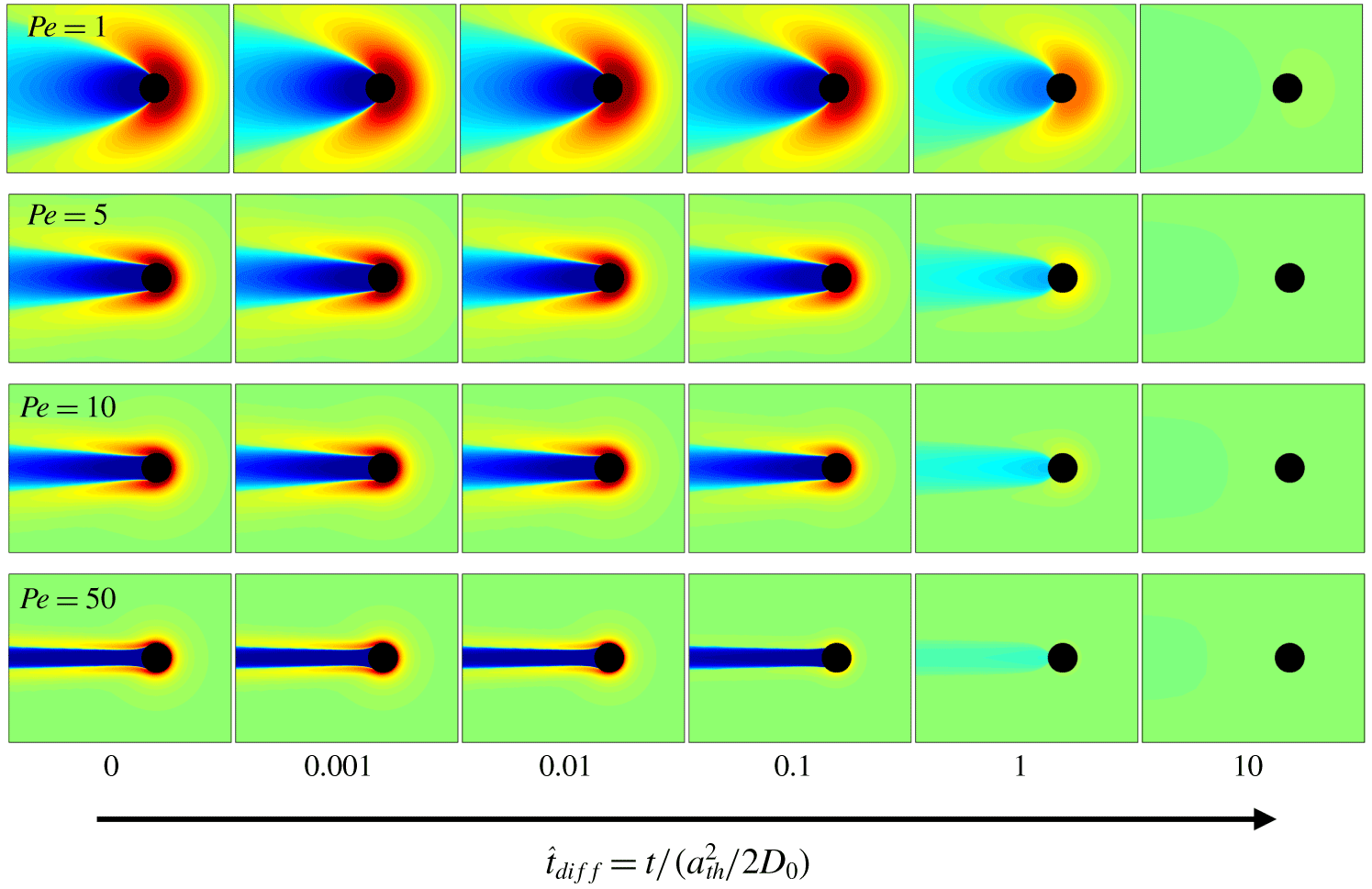
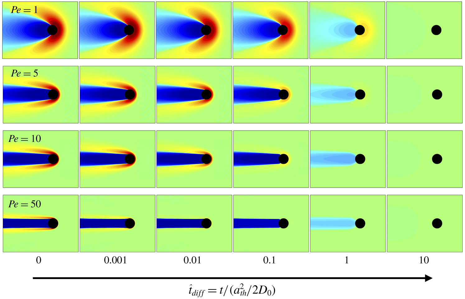
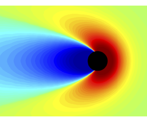
Contour plots showing relaxation of structural deformation around the probe after removal of the external force, with strong hydrodynamic interactions,  $\unicode[STIX]{x1D705}\rightarrow 0$, for
 $Pe=$ 1, 5, 10 and 50. Each image is a snapshot in time, scaled diffusively as shown at the bottom of the figure. The probe is at the centre of the black circle, which indicates the volume excluded to bath particle centres. Colour varies from red to green to blue for particle accumulation, undisturbed structure and particle depletion. Colour scaled for maximum contrast.

In this section, we examine structural relaxation after the removal of the external force driving the probe, at short and long times, and its effect on probe motion in the limit of very strong hydrodynamic interactions,  $\unicode[STIX]{x1D705}\rightarrow 0$. To understand how long structural deformation is remembered after shutoff of the external flow, we examine the contour plots of the relaxing structure at several instants in time after the force is removed. Contour plots of the relaxing microstructure,
 $f(\boldsymbol{r},t;\unicode[STIX]{x1D705}\rightarrow 0,Pe)$, obtained by numerical solutions of equations (2.18), are shown in figure 2, where the four rows correspond to pre-cessation forces
 $Pe=$ 1, 5, 10 and 50 (probe driven to the right in the plots). The black circle signifies the volume excluded to bath particle centres. Red shows bath particle accumulation (
 $f(\boldsymbol{r},t)>0$), blue represents depletion (
 $f(\boldsymbol{r},t)<0$) and green indicates an undisturbed structure (
 $f(\boldsymbol{r},t)=0$) around the probe. Since Brownian motion drives relaxation, time has been scaled diffusively as
 $t_{diff}=(a_{th}^{2}/2D_{0})$. The time corresponding to each of the snapshots is labelled at the bottom of the figure. Note that the colour scale is chosen for maximum contrast at each value of
 $Pe$, for best visual representation of structural gradients. Thus the density corresponding to dark red or dark blue differs from one value of
 $Pe$ to another.
Going down the left-most column ( $\hat{t}_{diff}=0$) of figure 2, the steady-state structural deformation for weak probe forcing is weak but propagates over long distances from the probe. In contrast, when forcing is strong, particle accumulation is concentrated at the upstream face of the probe and a depletion wake trails it, with very steep radial gradients in front of the probe and very steep lateral gradients across the trailing wake. Once the flow is shut off, Brownian motion acts to distribute the bath particles uniformly around the probe via random displacements and Brownian drift. For
 $Pe=1$ and
 $Pe=5$, the upstream and downstream regions appear to relax at the same rate. But for the more strongly distorted structure,
 $Pe=50$, the boundary layer appears to dissipate well before the wake fills in. The contour plots also indicate that the relaxation in the radial direction is faster than that in the angular direction, because angular gradients are weaker. This also influences filling-in of the wake, which occurs over long times. This is consistent with the theory and simulation results of Zia & Brady (Reference Zia and Brady2013), and later simulations by Marenne et al. (Reference Marenne, Morris, Foss and Brady2017), who examined the relaxation of a concentration suspension upon cessation of an external shear flow. In all cases, by the time it takes a particle to diffuse its size,
 $\hat{t}_{diff}=1$, the wakes in all four rows have mostly healed. This makes sense because the wake is approximately one particle size wide and lateral diffusion fills it in. But upstream relaxation is strongly dependent on pre-cessation
 $Pe$ – more strongly distorted structure at contact relaxes faster. This is consistent with the freely draining relaxation results of Zia & Brady (Reference Zia and Brady2013) discussed in § 3.1. However, comparison of the contour plots suggests that boundary-layer relaxation is slower when hydrodynamic interactions are stronger. This arises from the lubrication force at close particle distances that resists the separation of an interacting pair, and is illustrated in figure 3.
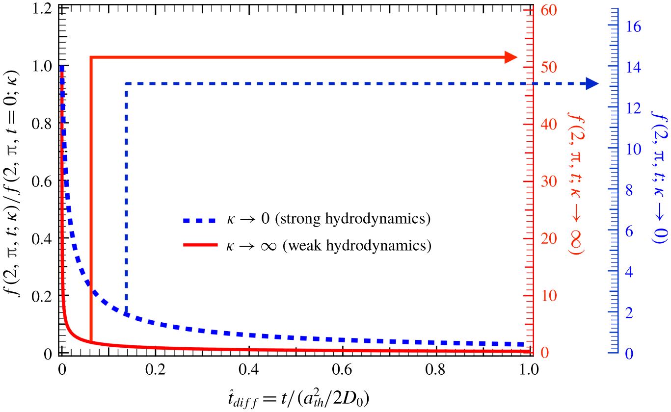
Stagnation-point density normalized by its value at  $\hat{t}_{diff}=0$ is plotted in the limits of weak (
 $\unicode[STIX]{x1D705}\rightarrow \infty$) and strong (
 $\unicode[STIX]{x1D705}\rightarrow 0$) hydrodynamic interactions on the left axis, revealing the faster rate of relaxation in the absence of hydrodynamics. The two right axes show the absolute value of the deformation at the stagnation point, revealing that a stronger deformation drives the faster relaxation rate. Note that the right axis for weak hydrodynamics (
 $\unicode[STIX]{x1D705}\rightarrow \infty$) spans
 $0\geqslant f\gtrsim 60$ and the right axis for strong hydrodynamics (
 $\unicode[STIX]{x1D705}\rightarrow 0$) spans only
 $0\gtrsim f\geqslant 16$.

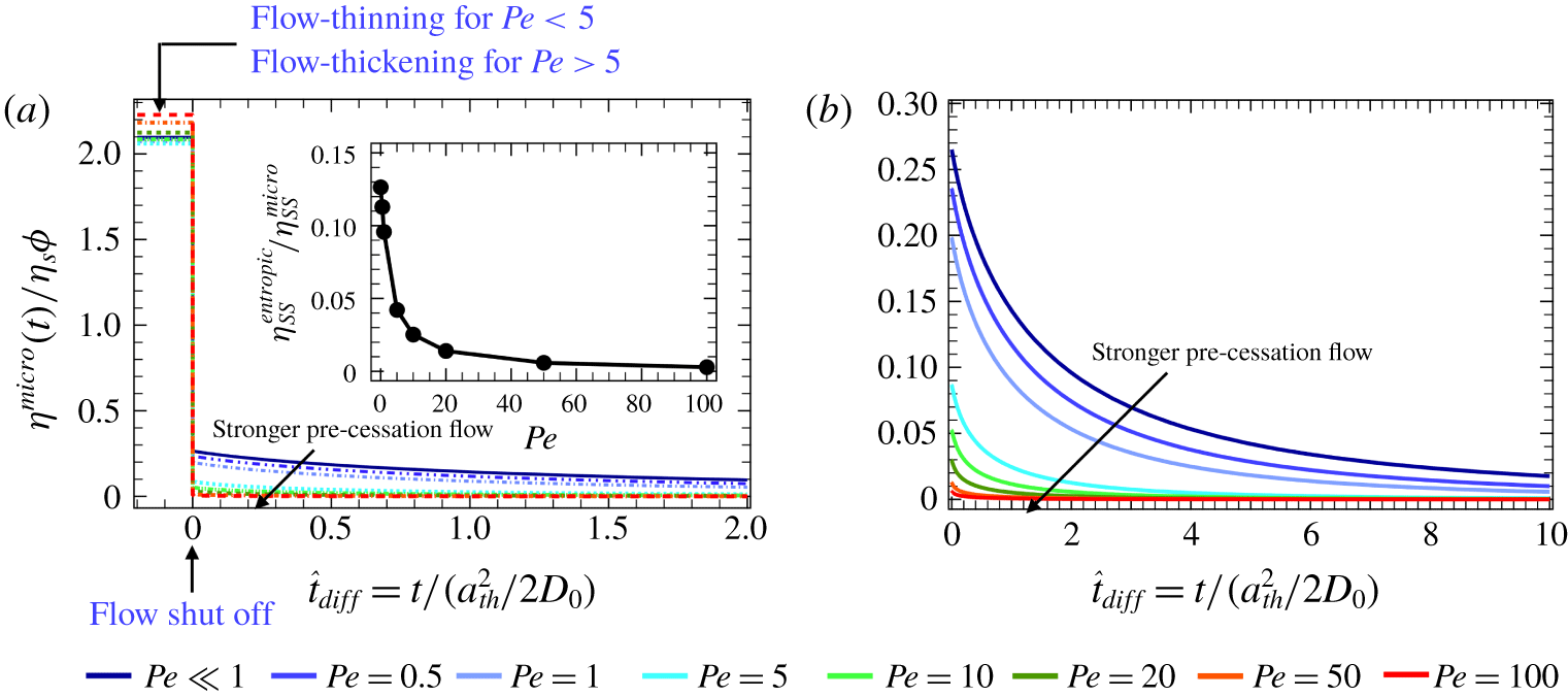
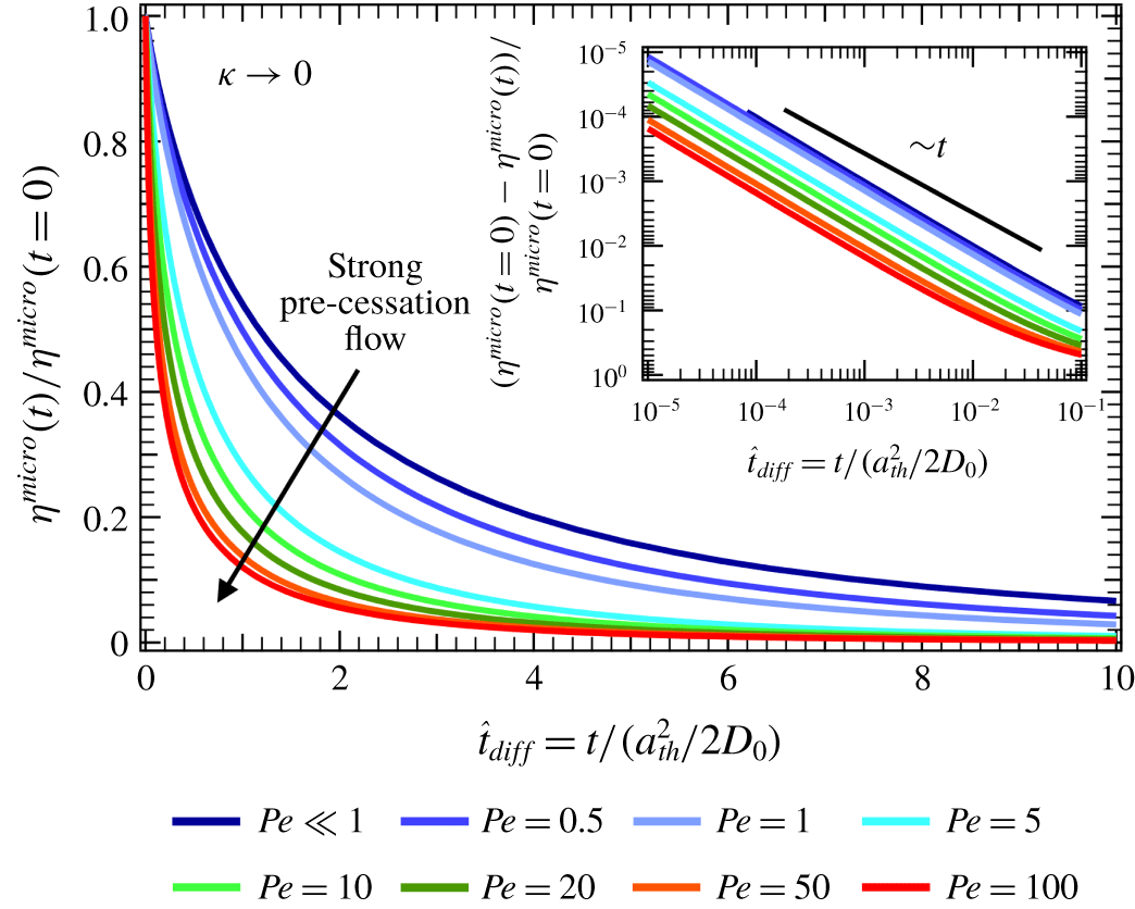
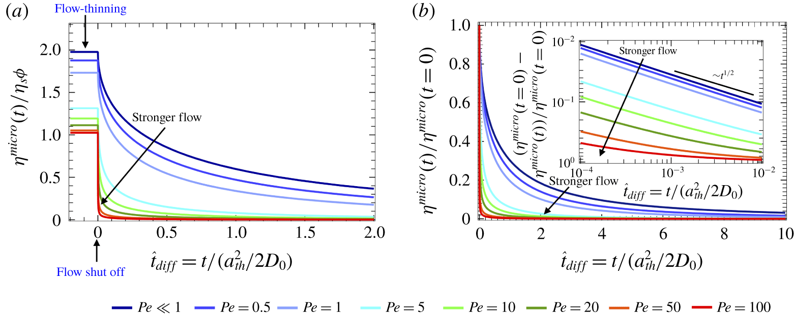
Flow cessation, strong hydrodynamics and arbitrary  $Pe$. (a) Microviscosity with diffusively scaled time for various pre-cessation
 $Pe$, where the external flow is shut off at
 $\hat{t}_{diff}=0$. (b) Decay of the entropic contributions to the viscosity after flow cessation.

Figure 3 shows the stagnation-point density, the structural distortion at the upstream face of the probe ( $r=2$ and
 $\unicode[STIX]{x1D703}=0$), in the limit of weak (
 $\unicode[STIX]{x1D705}\rightarrow \infty$, right axis) and strong (
 $\unicode[STIX]{x1D705}\rightarrow 0$, second right axis) hydrodynamic interactions (both at
 $Pe=50$) as a function of time. The steady-state structure prior to flow cessation is less distorted in the regime of strong hydrodynamic interactions. This weak gradient in the structure, along with the slower relative particle motion between particles in the presence of stronger hydrodynamic interactions, leads to a slower structural relaxation upon flow cessation. The strong impact of hydrodynamic interactions on the rate of structural relaxation will affect the probe motion, and in turn the viscosity of the colloidal dispersion. After the removal of the external force, deterministic probe motion arises solely from relaxation of the non-equilibrium structure (Zia & Brady Reference Zia and Brady2013). Hydrodynamic interactions slow this motion directly because they reduce relative particle mobility, and indirectly because they suppress microstructural distortion, leading to weaker gradients at a given value of
 $Pe$, and consequently slower relaxation.
We now examine the effect of structural relaxation on the viscosity. The solution in figure 2 is inserted in the viscosity expressions in equations (2.17) to obtain the decay in the viscosity with time, plotted in figure 4(a) as a function of diffusively scaled time for pre-cessation Péclet numbers ranging from 0.5 to 100, along with the asymptotically weak forcing limit,  $Pe\rightarrow 0$. As soon as the flow is shut off at
 $\hat{t}_{diff}=0$, there is an instantaneous and precipitous drop in the viscosity because the direct hydrodynamic contributions,
 $\unicode[STIX]{x1D702}^{H,0}$ and
 $\unicode[STIX]{x1D6FF}\unicode[STIX]{x1D702}^{H}$, vanish immediately. This intrinsic viscosity arising from the presence of the particles always remains, and pertains to relaxation of thermal fluctuations of
 $O(kT)$, but because it is intransient it exerts no effect on the cessation behaviour. We thus remove it from the plotted quantity. However, any viscous drag on the probe proportional to flow strength vanishes instantaneously upon flow shutoff, owing to the linearity of Stokes flow. Thus, any forces or velocities linear in
 $Pe$ vanish when flow is shut off.
This is not the case for interparticle forces and velocities, or for Brownian forces and velocities, because these care nothing about the flow, only relative particle positions. These forces produce random and deterministic relaxation after flow shutoff, the latter owing to structural gradients. Hydrodynamic interactions influence relative motion and slow this relaxation. In contrast, the non-equilibrium hydrodynamic contribution to the velocity and viscous drag (equation (2.17b)) is proportional to flow, and vanishes when flow ceases. This is no different from the corresponding contribution to the shear stress and shear viscosity, which vanishes instantaneously upon flow shutoff (Foss Reference Foss1999; Marenne et al. Reference Marenne, Morris, Foss and Brady2017). Subsequent evolution comes only from the entropic contributions to the steady-state viscosity,  $\unicode[STIX]{x1D702}^{P}$ and
 $\unicode[STIX]{x1D702}^{B}$, which relax monotonically in time, following structural relaxation (cf. figure 2).
An arrow indicates that the entropic contribution remaining after shutoff varies with  $Pe$, illustrated in the inset of figure 4(a), which plots the fraction of the total viscosity prior to shutoff that was entropic:
 $$\begin{eqnarray}\frac{\unicode[STIX]{x1D702}_{SS}^{entropic}}{\unicode[STIX]{x1D702}_{SS}^{micro}}=\frac{\unicode[STIX]{x1D702}_{SS}^{P}+\unicode[STIX]{x1D702}_{SS}^{B}}{\unicode[STIX]{x1D702}_{SS}^{micro}}.\end{eqnarray}$$
In the limit of weak external flow,  $Pe\ll 1$, and strong hydrodynamic interactions,
 $\unicode[STIX]{x1D705}\rightarrow 0$, one has
 $\unicode[STIX]{x1D702}_{SS}^{entropic}/\unicode[STIX]{x1D702}_{SS}^{micro}\rightarrow 0.128$, and since
 $\unicode[STIX]{x1D702}_{SS}^{P}+\unicode[STIX]{x1D702}_{SS}^{B}=0.128\unicode[STIX]{x1D702}_{SS}^{micro}=0.128\times 2.1\unicode[STIX]{x1D702}_{s}\unicode[STIX]{x1D719}=0.27\unicode[STIX]{x1D702}_{s}\unicode[STIX]{x1D719}$, we recover the steady-state results of Khair & Brady (Reference Khair and Brady2006). As the strength of the external force on the probe increases, the effect of Brownian motion gets weaker and, as a result, the entropic contribution to the steady-state viscosity decreases. This is reflected in the monotonic decrease of the relative entropic contribution,
 $\unicode[STIX]{x1D702}_{SS}^{entropic}/\unicode[STIX]{x1D702}_{SS}^{micro}$, with increasing
 $Pe$, shown in the inset of figure 4(a). While this ratio is easily calculated theoretically from steady-state analysis (Bergenholtz et al. Reference Bergenholtz, Brady and Vicic2002; Khair & Brady Reference Khair and Brady2006), such decomposition of the viscosity in experiments would be quite challenging. This illustrates the power of flow cessation to obtain the individual microscopic contributions to the steady-state viscosity.
Figure 4(b) shows the relaxation of only the entropic contributions to the steady-state viscosity as a function of diffusively scaled time for various strengths of pre-cessation external flow,  $Pe$. Flow-thickening behaviour that was present prior to flow cessation now vanishes as direct hydrodynamic contributions to the steady-state viscosity decay instantaneously upon flow cessation. However, hydrodynamic coupling between particles itself does not go away; it continues to influence the rate at which entropic contributions dissipate. We normalize the post-cessation viscosity with its value at
 $\hat{t}_{diff}=0$ and plot it as a function of time in figure 5. Curves for each
 $Pe$ exhibit at least two relaxation modes: initially viscosity relaxes at a fast rate, followed by a slower long-time decay. At very early times after shutoff, relaxation is linear in time,
 $$\begin{eqnarray}\frac{\unicode[STIX]{x1D702}^{micro}(t=0)-\unicode[STIX]{x1D702}^{micro}(t)}{\unicode[STIX]{x1D702}^{micro}(t=0)}\sim t\quad \text{as }t\rightarrow 0,\end{eqnarray}$$
suggesting that Brownian drift sets the early-time viscosity relaxation in the limit of strong hydrodynamic interactions,  $\unicode[STIX]{x1D705}\rightarrow 0$ (inset in figure 5). This makes a stronger statement however: the early-time rate of viscosity decay is independent of the pre-cessation flow strength,
 $Pe$. The
 $Pe$ independence of the relaxation is also found in the limit of weak hydrodynamic interactions,
 $\unicode[STIX]{x1D705}\rightarrow \infty$ (see appendix A). Comparing figure 5 and figure 14 (in appendix A) shows that hydrodynamics slows the rate of relaxation. When
 $\unicode[STIX]{x1D705}\rightarrow 0$,
 $\unicode[STIX]{x1D702}^{micro}\sim t$ at
 $t\rightarrow 0$, but when
 $\unicode[STIX]{x1D705}\rightarrow \infty$,
 $\unicode[STIX]{x1D702}^{micro}\sim t^{1/2}$. This hydrodynamic coupling persists over the entire relaxation process, slowing the long-time relaxation – irrespective of the pre-cessation
 $Pe$. This is discussed in § 3.3.
Normalization of post-cessation entropic viscosity on its initial value reveals multiple relaxation processes, regardless of pre-cessation  $Pe$. Inset: early-time decay is advective. Strong hydrodynamics (
 $\unicode[STIX]{x1D705}\rightarrow 0$).

The relaxation rate also depends on pre-cessation flow strength, with faster relaxation after stronger flow. This behaviour is similar to the relaxation observed in shear rheology flow cessation for concentrated suspensions (Foss Reference Foss1999; Marenne et al. Reference Marenne, Morris, Foss and Brady2017) and microrheological flow cessation in the absence of hydrodynamic interactions (Zia & Brady Reference Zia and Brady2013). To examine the micromechanical origins of this behaviour, we recall that stronger flow produces more localized distortion and stronger asymmetry as long as  $\unicode[STIX]{x1D705}\neq 0$ (Batchelor Reference Batchelor1976; Khair & Brady Reference Khair and Brady2006; Chu & Zia Reference Chu and Zia2016). Strong flow produces a boundary layer that gets compressed as flow strength increases, with a thickness that scales as
 $\unicode[STIX]{x1D6FF}\sim 1/Pe$ (Squires & Brady Reference Squires and Brady2005). The densest region of the boundary layer is at the contact stagnation point,
 $f(2,\unicode[STIX]{x03C0},t)$, which increases with increasing
 $Pe$. Together, these drive a strong particle gradient across the boundary layer. To relax it, the probe need only diffuse a distance
 $\unicode[STIX]{x1D6FF}\sim 1/Pe$, and a stronger gradient produces a faster push to do so (Zia & Brady Reference Zia and Brady2013). This is quantified in figure 6.
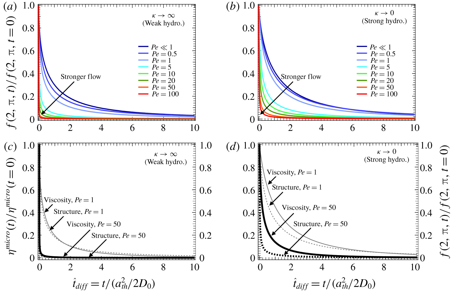
Comparison of structural relaxation rates to viscosity relaxation rate, with and without hydrodynamic interactions. (a,b) Structural relaxation at the stagnation point for (a) weak and (b) strong hydrodynamics. (c,d) Viscosity (on left axes) and stagnation-point density (on right axes) for (c) weak and (d) strong hydrodynamics. Panel (c) shows that, in a freely draining system, structure and rheology relax at the same rate. However, when hydrodynamics are strong (d), stagnation-point density relaxation leads viscosity relaxation. This illustrates one role of long-range hydrodynamics in viscosity relaxation, where downstream coupling in the more slowly relaxing wake region slows probe motion.

The maximum boundary-layer density, which occurs at the stagnation point,  $f(2,\unicode[STIX]{x03C0},t)$, normalized by its initial value, is plotted as it decays with time for various values of
 $Pe$ in the limits of weak (
 $\unicode[STIX]{x1D705}\rightarrow \infty$) and strong (
 $\unicode[STIX]{x1D705}\rightarrow 0$) hydrodynamic interactions in figure 6(a) and (b), respectively. These plots show the presence of multiple relaxation time scales with or without hydrodynamics: an early-time fast relaxation followed by a long-time slower decay (Zia & Brady Reference Zia and Brady2013). The relaxation of the stagnation-point density is faster with increasing
 $Pe$ – irrespective of
 $\unicode[STIX]{x1D705}$ – showing that a more deformed structure relaxes faster, which owes its origin to boundary-layer dynamics, discussed further below. We next compare the relaxation rate of viscosity versus the relaxation rate of structure, for two representative flow strengths,
 $Pe=1$ and
 $Pe=50$. In figure 6(c) and (d), we plot the viscosity (left axis) versus the stagnation-point density (right axis), for weak (c) and strong (d) hydrodynamics. In the freely draining system (figure 6c), structure and viscosity relax at the same rate, irrespective of
 $Pe$, confirming the idea that contact structure sets the viscosity relaxation in the limit of
 $\unicode[STIX]{x1D705}\rightarrow \infty$ (Zia & Brady Reference Zia and Brady2013). In contrast, when hydrodynamic interactions matter (figure 6d), the stagnation-point density relaxes faster than the viscosity; this arises from long-ranged hydrodynamic interactions, where a particle that has relaxed away from contact still interacts with the probe through solvent-mediated hydrodynamic interactions. This illustrates one role of long-range hydrodynamics in viscosity relaxation, where downstream coupling in the more slowly relaxing wake region slows probe motion.
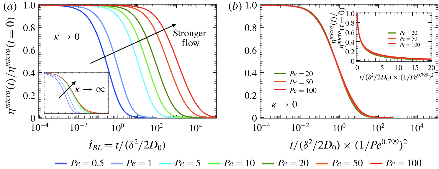
Flow cessation for strong hydrodynamics and arbitrary  $Pe$. (a) Normalized microviscosity as a function of
 $\hat{t}_{BL}=t/(\unicode[STIX]{x1D6FF}^{2}/2D_{0})$. For comparison, the weak hydrodynamics behaviour (
 $\unicode[STIX]{x1D705}\rightarrow \infty$) is shown in the inset. Comparison of the two reveals that, when relaxation time is scaled on the diffusivity of a particle on the length scale
 $\unicode[STIX]{x1D6FF}\sim 1/Pe$ of the boundary layer, only in the absence of hydrodynamics (inset) do the curves collapse at high
 $Pe$. This suggests that the scaling of particle mobility, rather than just the distance travelled to relax the boundary layer, must be taken into account. (b) The diffusivity is rescaled with the
 $Pe$-dependent concentration in the boundary layer, where now the curves align for all
 $Pe$.

We now take a closer look at the relaxation time scale that evidently changes with structural deformation. In studies of freely draining suspensions, a simple rescaling of time – where the diffusive process setting relaxation occurs through the boundary layer – collapses viscosity relaxation curves together, for values of  $Pe$ sufficiently high to produce a proper boundary layer. Similar rescalings have been applied in hydrodynamically interacting systems with varying degrees of success (Foss Reference Foss1999; Marenne et al. Reference Marenne, Morris, Foss and Brady2017). The idea is that the probe need execute only one diffusive step out of the wake to relax the majority of the suspension stress. In figure 7(a), the post-cessation viscosity is scaled on the boundary-layer thickness,
 $\unicode[STIX]{x1D6FF}\sim 1/Pe$ (Khair & Brady Reference Khair and Brady2006), but fails to unite any of the curves. However, the rescaling works quite well at high
 $Pe$ in the freely draining system (inset), a phenomenon that has also been observed in sheared suspensions (Foss Reference Foss1999; Marenne et al. Reference Marenne, Morris, Foss and Brady2017). The difference between the two is the density inside the boundary layer, which is
 $g\sim Pe$ for freely draining (Squires & Brady Reference Squires and Brady2005) and
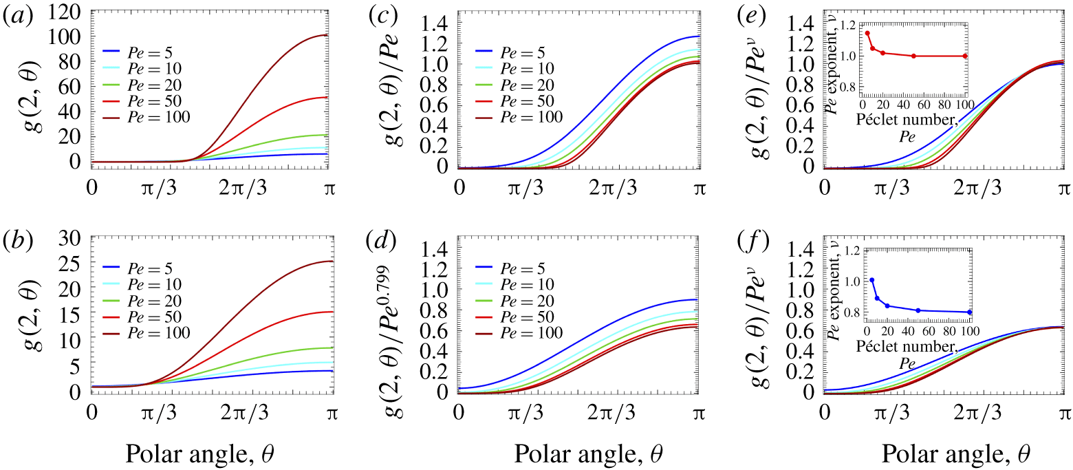
 $g\sim Pe^{\unicode[STIX]{x1D708}}$, with
 $\unicode[STIX]{x1D708}=0.799$, for strong hydrodynamics (Khair & Brady Reference Khair and Brady2006). Thus it makes sense to rescale not only the distance the probe must travel as it diffusively relaxes, but also the diffusive hindrance. That is, the boundary layer is less crowded, although hydrodynamic coupling slows relative motion there. We rescale time on the hindered diffusion in figure 7(b), where the high-
 $Pe$ viscosity curves are plotted as a function of time made dimensionless on boundary-layer relaxation,
 $t/(\unicode[STIX]{x1D6FF}^{2}/2D_{0})\times (1/Pe^{0.799})^{2}$. This reflects the time required for a particle to diffuse the thickness
 $\unicode[STIX]{x1D6FF}$ of a boundary layer of density
 $g\sim Pe^{\unicode[STIX]{x1D708}}$, where
 $\unicode[STIX]{x1D708}=0.799$ for
 $\unicode[STIX]{x1D705}=0$ (Khair & Brady Reference Khair and Brady2006). This scaling effectively adjusts the diffusive relaxation process for both boundary-layer hindrance
 $g\sim Pe^{\unicode[STIX]{x1D708}}$ and the distance
 $\unicode[STIX]{x1D6FF}$ the probe must travel to relax it. This collapses the high-
 $Pe$ curves together quite well in figure 7(b). The rescaling argument depends on the formation of a thin boundary layer through which the probe must execute a diffusive step to relax both structure and stress, making this scaling most appropriate when
 $Pe$ is appropriately large.
This analysis provides a direct way to compare the effective boundary-layer thickness in the presence of strong hydrodynamic interactions to the regime of weak hydrodynamics,  $\unicode[STIX]{x1D6FF}(\unicode[STIX]{x1D705}\rightarrow 0)\approx Pe^{0.799}\times \unicode[STIX]{x1D6FF}(\unicode[STIX]{x1D705}\rightarrow \infty )$. This further emphasizes the importance of the boundary layer in the relaxation behaviour in dilute suspensions. The probe need move only the size of the boundary layer to relax the majority of the stress. However, for concentrated suspensions, the particle gradient across the wake will also play a prominent role in the relaxation process in both microrheology (Zia & Brady Reference Zia and Brady2013) and shear macrorheology (Foss Reference Foss1999; Marenne et al. Reference Marenne, Morris, Foss and Brady2017). The important implication of the difference between the strong hydrodynamics (main plot in figure 7a) and freely draining limits (inset in figure 7a) is that, even though the hydrodynamic contribution arising directly from the imposed flow vanishes immediately upon flow cessation, its impact on particle mobility and structural deformation persists well after flow shutoff.
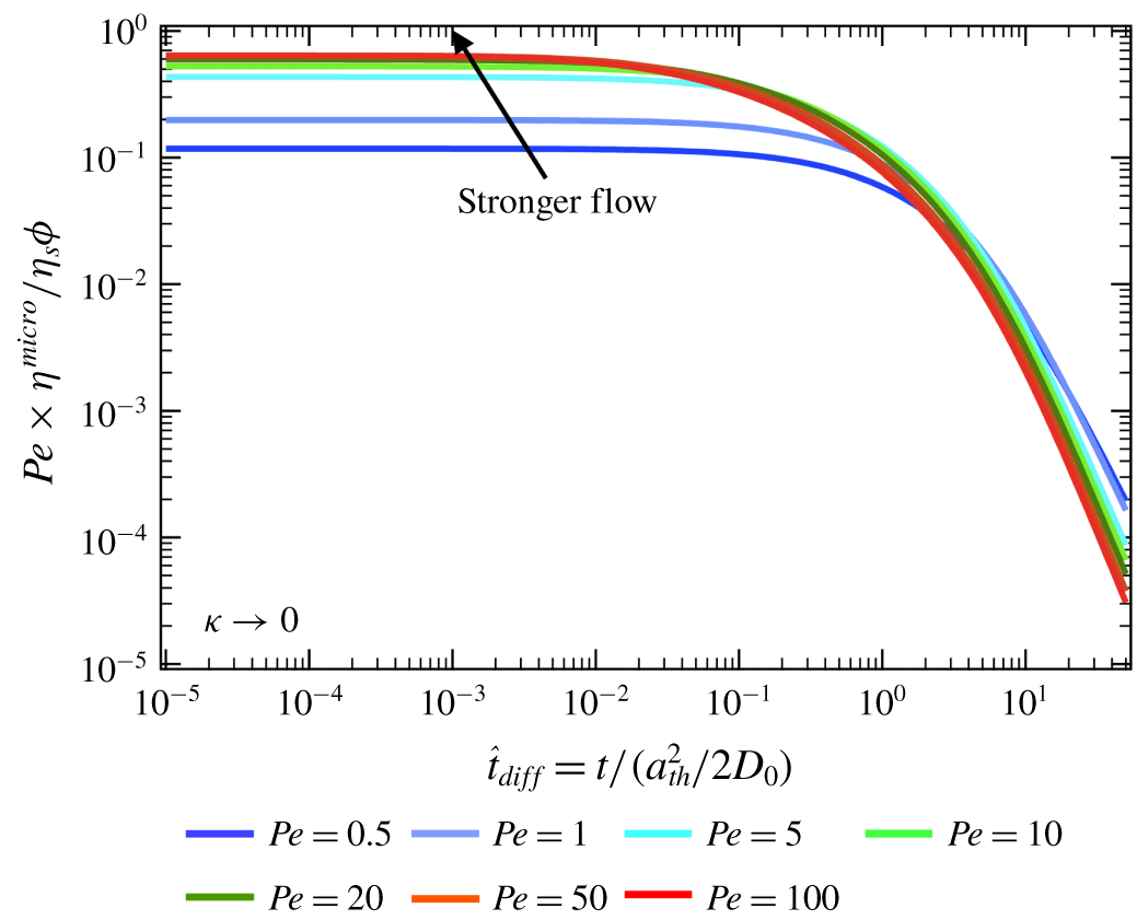
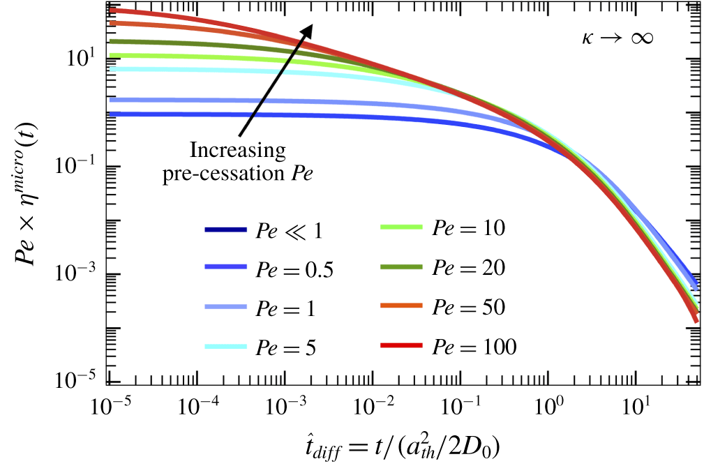
Flow cessation, strong hydrodynamics and arbitrary  $Pe$: viscosity has been multiplied by the pre-cessation
 $Pe$ and is plotted against the diffusively scaled time.

The relaxation behaviour upon flow cessation gives the extent to which microstructural distortions persist in suspensions and memory behaviour in colloidal dispersions. We further examine the long-time viscosity relaxation over diffusive time scales in figure 8, where the viscosity is multiplied by  $Pe$ (giving a measure of the stress associated with the deformed microstructure) and is plotted as a function of the diffusively scaled time for various
 $Pe$ in the limit of strong hydrodynamic interactions,
 $\unicode[STIX]{x1D705}\rightarrow 0$. Since the steady-state viscosities at different
 $Pe$ are of the same order, the vertical axis in figure 8 gives a measure of how far the structure is driven from its equilibrium configuration prior to flow cessation (Foss Reference Foss1999; Zia & Brady Reference Zia and Brady2013; Marenne et al. Reference Marenne, Morris, Foss and Brady2017). Earlier we established that the early-time viscosity decay is set by the boundary-layer relaxation, whereas the long-time viscosity relaxation reflects the structural rearrangement as Brownian motion drives the particles towards a uniform distribution. At long times, all the curves in figure 8, corresponding to different pre-cessation
 $Pe$, align well with each other, signalling the loss of memory in the distorted suspension. This behaviour is similar to that found in the regime of weak hydrodynamic interactions (Zia & Brady Reference Zia and Brady2013) and suggests that, independent of the initial distortion, the microstructural relaxation follows the same path at long times even for colloidal particles interacting via strong hydrodynamic interactions. The early-time relaxation is faster with increasing
 $Pe$, and therefore the time at which the curves begin to follow the long-time relaxation behaviour decreases with increasing
 $Pe$, signalling a decrease in the duration of memory in the colloidal dispersion. This also indicates that the memory is stored entropically in the distorted microstructure, which will be further explored in § 3.4. The loss of memory at long times recovers previous results of microrheology (Zia & Brady Reference Zia and Brady2013) and shear rheology (Foss Reference Foss1999; Marenne et al. Reference Marenne, Morris, Foss and Brady2017).
In summary, hydrodynamic interactions slow all modes of structural relaxation because such coupling slows relative particle motion. But the same interactions preserve structural symmetry pre-cessation and the two effects combined produce qualitatively different relaxation than that found in a freely draining suspension. The most distinct of these effects is the long-range hydrodynamic coupling that wraps structure around the probe, providing a pronounced temporal lag of rheological relaxation behind structural relaxation in the boundary layer – in contrast to freely draining systems where the two relax together. Flow thickening is forgotten instantaneously after flow shutoff, reaffirming the hydrodynamic nature of that phenomenon.
3.3 Arbitrary forcing and strength of hydrodynamics
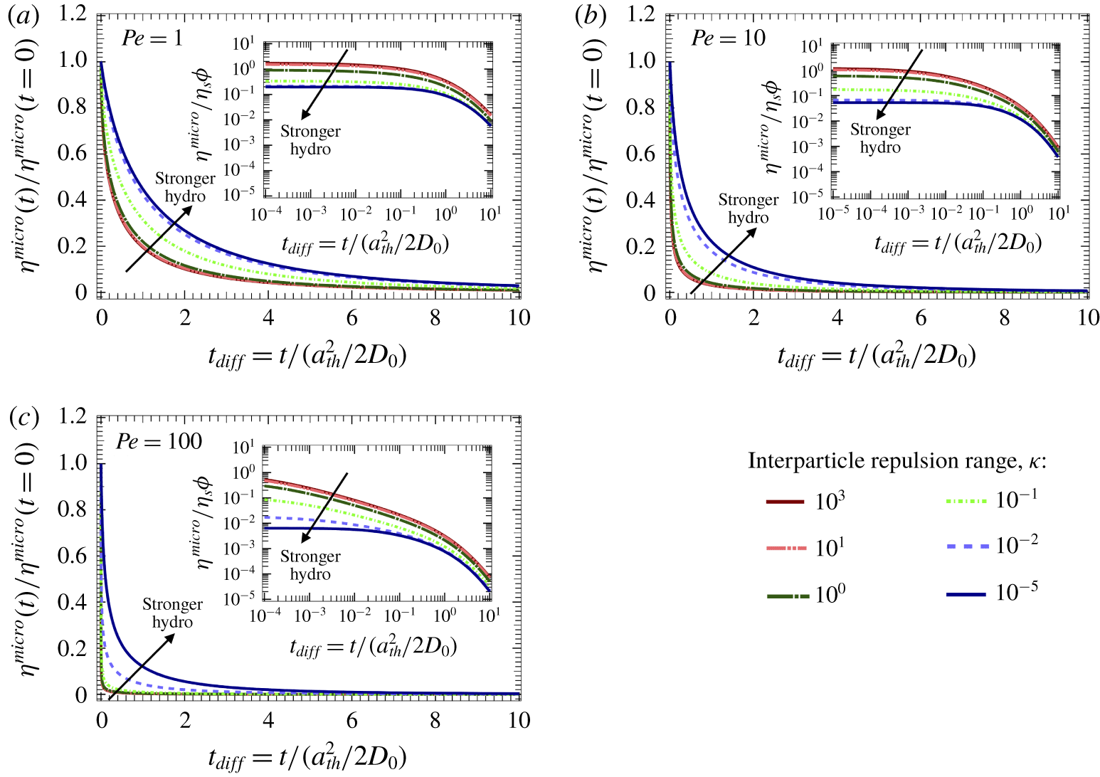
Normalized viscosity as a function of time for a range of  $\unicode[STIX]{x1D705}$ for (a)
 $Pe=1$, (b)
 $Pe=10$ and
 $Pe=100$. The insets show the absolute values of the viscosity in a log–log plot to focus on the early-time relaxation and long-time algebraic decay.

Real materials in industry and science are typified by intermediate flow strengths and particle surface conditions that give moderately strong hydrodynamic interactions. Here we study relaxation at these finite values of  $Pe$ and
 $\unicode[STIX]{x1D705}$. In figure 9, we plot the normalized viscosity as a function of the diffusively scaled time after flow shutoff, for
 $\unicode[STIX]{x1D705}\in [10^{-5},10^{3}]$, with one value of
 $Pe$ in each plot:
 $Pe=1$,
 $Pe=10$ and
 $Pe=100$. All three plots show at least two relaxation modes: an early-time faster relaxation, which becomes more pronounced with increasing
 $Pe$, and a slower long-time decay of
 $\unicode[STIX]{x1D702}^{micro}$ towards zero. All relaxation modes slow down as hydrodynamic interactions become stronger, because they slow relative diffusion. However, the viscosity relaxes back to equilibrium faster with increasing pre-cessation
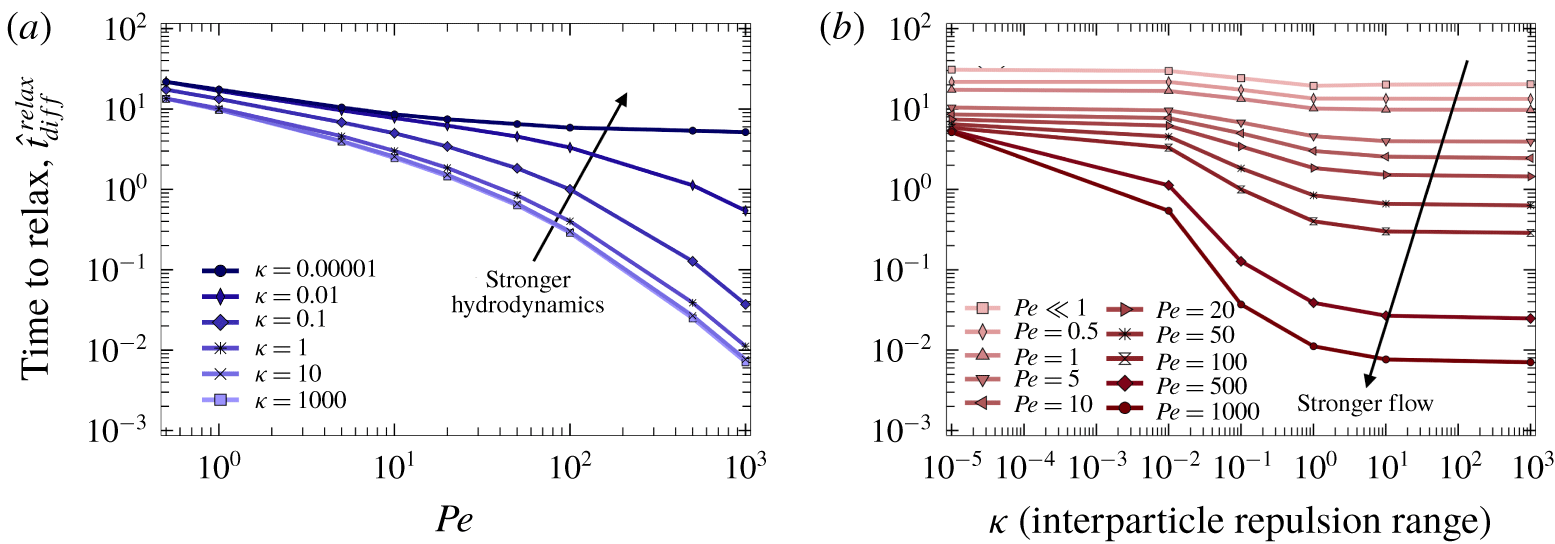
 $Pe$. We expect the latter based on the asymptotic results in the previous section, but here we analyse it quantitatively, with a focus on the time required for the microviscosity to completely relax,
 $\hat{t}_{diff}^{relax}$, in detail.
In figure 10(a), we plot  $\hat{t}_{diff}^{relax}$ as a function of the pre-cessation probe forcing,
 $Pe$, for various strengths of hydrodynamic interactions between particles,
 $\unicode[STIX]{x1D705}$. Relaxation is faster following higher-
 $Pe$ flow (at fixed
 $\unicode[STIX]{x1D705}$), but this effect weakens as hydrodynamic interactions grow stronger and hinder diffusive relaxation.
Time required for the viscosity to fully relax,  $\hat{t}_{diff}^{relax}$, as a function of (a)
 $Pe$ for various
 $\unicode[STIX]{x1D705}$, and of (b)
 $\unicode[STIX]{x1D705}$ for various
 $Pe$.

The parameter space is ‘flipped’ in figure 10(b) to highlight the primary effects of hydrodynamic coupling on structural relaxation. First, hydrodynamics preserve symmetry, which suppresses the strong gradients that drive fast relaxation. Second, they impede relative particle motion. These two effects combined slow down structural and rheological relaxation. For higher pre-cessation flow, these effects become more pronounced, approaching the pure hydrodynamics limit where structure is symmetric and Brownian motion is absent, removing all mechanisms for relaxation. As a result  $\unicode[STIX]{x1D705}$ has a very strong effect on
 $\hat{t}_{diff}^{relax}$ as pre-cessation
 $Pe$ increases.
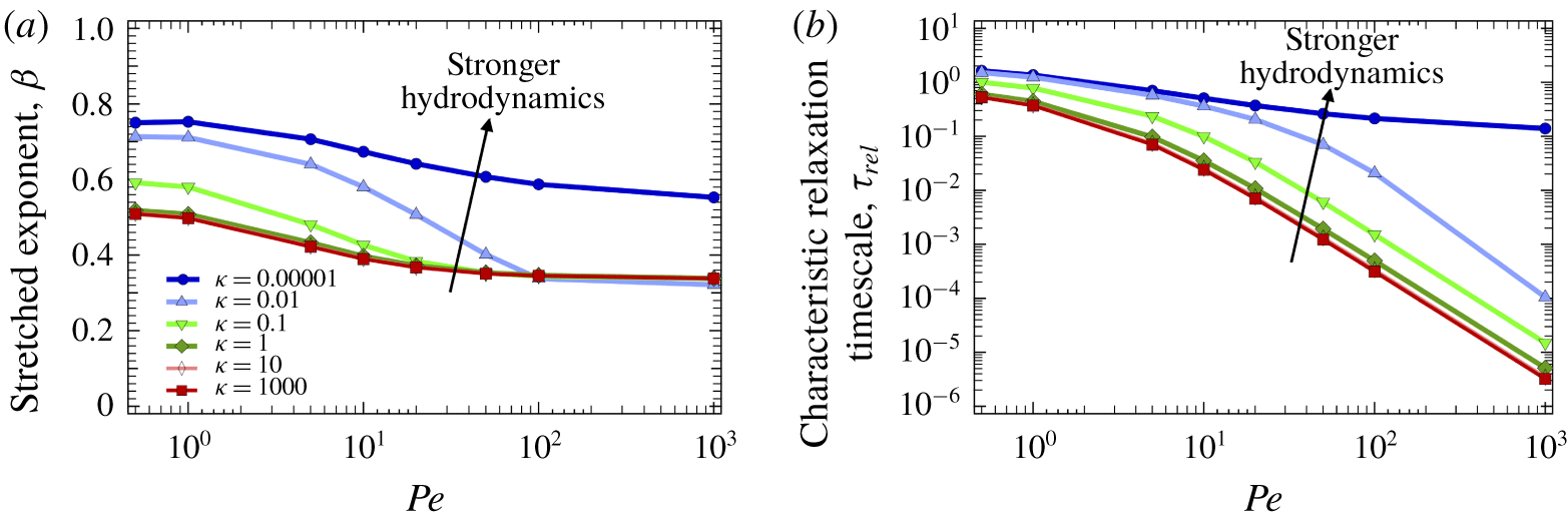
Flow cessation, arbitrary  $Pe$ and
 $\unicode[STIX]{x1D705}$: (a) stretched exponent,
 $\unicode[STIX]{x1D6FD}$, as a function of
 $Pe$ for various values of
 $\unicode[STIX]{x1D705}$, and (b) characteristic relaxation time scale,
 $\unicode[STIX]{x1D70F}_{rel}$, as a function of
 $Pe$ for various strengths of hydrodynamic interactions.

Relaxation processes are sometimes fitted to a stretched exponential following the Kohlrausch–Williams–Watts function form (Bouchaud Reference Bouchaud2008):
 $$\begin{eqnarray}\frac{\unicode[STIX]{x1D702}^{micro}}{\unicode[STIX]{x1D702}^{micro}(t=0)}\sim \text{e}^{-(t/\unicode[STIX]{x1D70F}^{rel})^{\unicode[STIX]{x1D6FD}}}.\end{eqnarray}$$
This functional form can be solved for both the stretching exponent,  $\unicode[STIX]{x1D6FD}$, and the characteristic relaxation time scale,
 $\unicode[STIX]{x1D70F}_{rel}$. The stretching exponent,
 $0\leqslant \unicode[STIX]{x1D6FD}\leqslant 1$, indicates a disparity in the different rates at which a system relaxes. For a system with one relaxation process (or one relaxation time scale),
 $\unicode[STIX]{x1D6FD}=1$, and
 $\unicode[STIX]{x1D6FD}$ decreases if a structure relaxes over multiple disparate time scales. Prior cessation relaxation studies of sheared suspensions mention that, in the limit of very strong hydrodynamic interactions,
 $\unicode[STIX]{x1D70F}_{rel}$ and
 $\unicode[STIX]{x1D6FD}$ both decrease monotonically with increasing
 $Pe$ (Marenne et al. Reference Marenne, Morris, Foss and Brady2017). Here we seek a mechanistic explanation for this behaviour. We fit the data in figure 9 to equation (3.3) and plot the stretching exponent,
 $\unicode[STIX]{x1D6FD}$, in figure 11(a), for several values of
 $\unicode[STIX]{x1D705}$, and the characteristic relaxation time scale,
 $\unicode[STIX]{x1D70F}_{rel}$, in figure 11(b). Our work recovers the
 $Pe$-dependent behaviour found in sheared suspensions, and additionally finds that both
 $\unicode[STIX]{x1D6FD}$ and
 $\unicode[STIX]{x1D70F}_{rel}$ increase monotonically with decreasing
 $\unicode[STIX]{x1D705}$ (strengthening hydrodynamic interactions), supporting our conclusion that hindered relative mobility in the boundary layer slows stress relaxation. The stretched exponent,
 $\unicode[STIX]{x1D6FD}$ in figure 11(a), decreases with increasing
 $Pe$, indicating the disparity between the early-time faster and long-time slower relaxation processes for high
 $Pe$ (Zia & Brady Reference Zia and Brady2013). With increasing strength of hydrodynamic interactions, the disparity between the faster and slower relaxation modes decreases, leading to a larger
 $\unicode[STIX]{x1D6FD}$.
3.4 Probe motion and non-equilibrium osmotic pressure
Non-equilibrium osmotic pressure drives deterministic probe motion after the external force has been removed. (a) The probe displacement (left axis) and the steady-state osmotic pressure (right axis) from Chu & Zia (Reference Chu and Zia2017, with permission), as a function of  $Pe$. (b) Ratio of the pre-cessation osmotic pressure to the probe displacement as a function of
 $Pe$.

In the previous sections, we examined the viscous behaviour of colloidal dispersions with a focus on the relaxation of the viscosity upon flow cessation. Here, we explore the elastic behaviour in suspensions by examining the stress and energy storage in a distorted microstructure, and their effect on particle motion. At equilibrium, thermal fluctuations produce temporary gradients in number density that relax via Brownian diffusion, giving rise to osmotic pressure. The reduction in entropy associated with local compression of structure temporarily stores energy entropically, but this chemical potential is quickly dissipated viscously back into the solvent. Zia & Brady (Reference Zia and Brady2013) showed that flow energy stored entropically in the steady-state deformed microstructure can be partially recovered to deterministically back-drive the probe after removal of the external force, for a freely draining suspension. When hydrodynamic interactions play a role, the compressed boundary layer, and the rate at which it relaxes, change (cf. §§ 3.2 and 3.3). Here we investigate whether hydrodynamics changes the useful work the non-equilibrium osmotic pressure can do post-cessation. We monitor probe position after removal of the external force, and plot the total probe displacement,  $\langle x\rangle (Pe,\unicode[STIX]{x1D705})$, where the angle brackets signify an average over realizations, on the left axis in figure 12(a). When pre-cessation
 $Pe$ is small, very little deterministic probe motion occurs after cessation, because the relaxing structure was a weak diffusive dipole. As
 $Pe$ increases, the same trend as observed in freely draining systems (Zia & Brady Reference Zia and Brady2013) is observed: probe displacement grows. However, the stronger the hydrodynamic interactions, the less post-cessation total displacement at any fixed
 $Pe$. The preservation of structural symmetry by hydrodynamic interactions is responsible for this behaviour. But as
 $Pe$ continues to grow, total displacement actually decreases, because now the boundary layer has wrapped around the probe, accumulating particles in the downstream region of the probe. The probe thus gets a more symmetric distribution of kicks from behind as well as in front, and, in consequence, the osmotic force is more uniformly distributed on the probe. The probe displacement now decreases with increasing
 $Pe$. From an entropic perspective, a less distorted structure stores less energy.
The strength of hydrodynamic interactions between particles,  $\unicode[STIX]{x1D705}$, has a strong influence on the steady-state structure around the probe, and in turn on the average probe displacement after flow cessation. Stronger hydrodynamic coupling preserves symmetry, leading to a weaker entropic force, and thence less average probe displacement. Overall, while the total mean probe displacement upon flow cessation decreases with increasing strength of hydrodynamic interactions,
 $\unicode[STIX]{x1D705}$, it shows a non-monotonic dependence on the pre-cessation probe forcing strength,
 $Pe$, owing to the wrapping of the boundary layer around the probe.
Since the probe motion after flow cessation arises solely from the deformed structure, one can connect the entropic force that drives the probe with the osmotic compressibility of the suspension (Zia & Brady Reference Zia and Brady2013). The steady-state osmotic pressure was calculated by Chu & Zia (Reference Chu and Zia2017) as a function of  $Pe$ for various values of
 $\unicode[STIX]{x1D705}$ and we plot those values on the right axis in figure 12(a). A comparison between the post-cessation mean probe displacement,
 $\langle x\rangle (Pe,\unicode[STIX]{x1D705})$, and the non-equilibrium osmotic pressure,
 $\langle \unicode[STIX]{x1D6F1}^{neq}\rangle (Pe,\unicode[STIX]{x1D705})$, reveals that the two quantities are strongly correlated: both
 $\langle x\rangle (Pe,\unicode[STIX]{x1D705})$ and
 $\langle \unicode[STIX]{x1D6F1}^{neq}\rangle (Pe,\unicode[STIX]{x1D705})$ approach zero as
 $Pe\ll 1$, both increase with increasing
 $Pe$ for
 $Pe<5$ and decrease thereafter; for weak hydrodynamic interactions, both quantities approach an asymptotic value at very high
 $Pe$. Increasing strength of hydrodynamic coupling between particles suppresses both
 $\langle x\rangle (Pe,\unicode[STIX]{x1D705})$ and
 $\langle \unicode[STIX]{x1D6F1}^{neq}\rangle (Pe,\unicode[STIX]{x1D705})$ at all
 $Pe$. In the limit of strong hydrodynamic interactions,
 $\unicode[STIX]{x1D705}\rightarrow 0$, and strong probe forcing,
 $Pe$, both quantities approach zero. This behaviour in the dual limits of strong hydrodynamic interactions and strong probe forcing is expected, as these asymptotic limits correspond to the pure Stokes flow limit, where the structure becomes spherically symmetric around the probe particle. This symmetric structure leads to zero mean probe displacement upon removal of the external force.
Overall, both the probe back-travel,  $\langle x\rangle (Pe,\unicode[STIX]{x1D705})$, and the steady-state osmotic pressure,
 $\langle \unicode[STIX]{x1D6F1}^{neq}\rangle (Pe,\unicode[STIX]{x1D705})$, are attenuated by hydrodynamic interactions, and exhibit a non-monotonic behaviour in
 $Pe$ associated with wrapping of the boundary layer. There is a strong one-to-one qualitative connection between the osmotic pressure and probe back-travel. In fact, the ratio is near unity when hydrodynamic interactions are strong, which is more clearly seen in figure 12(b) where we plot the ratio of the osmotic pressure to the probe back-travel as a function of
 $Pe$ for various
 $\unicode[STIX]{x1D705}$. This ratio, which signifies the entropic force density arising from the distorted structure, exhibits a strong dependence on the strength of hydrodynamic interactions,
 $\unicode[STIX]{x1D705}$. However, this ratio does not change much as
 $Pe$ is varied, suggesting that the probe back-travel gives a very clear experimental measure of the osmotic pressure in a suspension. This further illustrates that the stored energy can do useful work and the probe back-travel gives a direct measure of the flow energy density associated with the deformed structure.
In summary, probe back-travel upon flow cessation can provide a measure of the osmotic pressure in a colloidal dispersion, a link inferred from the connection of the osmotic pressure to the chemical potential. The osmotic pressure is energy density stored entropically in the distorted hard-sphere suspension. Hydrodynamic interactions hinder this entropic energy storage in colloidal dispersions by preserving structural symmetry and, in addition, they reduce the useful work available upon flow cessation by hindering relative particle motion.
4 Conclusions
We have presented a detailed study of the impact of hydrodynamic and entropic interactions on the relaxation behaviour of hard-sphere colloidal suspensions, utilizing the theoretical framework of active microrheology. Colloidal dispersions exhibit non-Newtonian rheological behaviours owing to sustained distortions in their microstructure when under an applied external flow. Upon sudden removal of the external flow, the structural distortions are dissipated by Brownian motion of the particles. The rate of the structural relaxation is set by the relative strengths of microscopic forces, viz. hydrodynamic, entropic and other interparticle forces. In this study, we utilized an excluded-annulus model to systematically tune the relative strengths of hydrodynamic to entropic forces, and examine how quickly they heal microstructural distortions.
We find that hydrodynamic interactions slow all modes of structural relaxation because such coupling slows relative particle motion. But the same action of hydrodynamic interactions preserves structural symmetry pre-cessation, and the two effects combined produce qualitatively different relaxation than that found in a freely draining suspension. Early relaxation is linear in time when hydrodynamics matter, and is driven by Brownian drift as the probe seeks configurations of higher mobility. In contrast, relaxation of a freely draining dispersion is faster, scaling with the square root of time. These behaviours owe their origin to changes in structure that persist after forcing is removed.
The most distinct of these effects is the long-range hydrodynamic coupling that wraps structure around the probe, providing a pronounced temporal lag of rheological relaxation behind structural relaxation – in contrast to freely draining systems where the two relax together. Examination of cessation behaviour with variation in pre-cessation flow strength  $Pe$ shows that stronger flow leads to faster post-cessation relaxation, but this behaviour is mitigated as hydrodynamic interactions grow stronger. Hydrodynamic interactions preserve memory longer, driving longer relaxation times regardless of initial flow strength. However, flow thickening is forgotten instantaneously after flow shutoff, reaffirming the hydrodynamic nature of that phenomenon.
Between the pure hydrodynamic and freely draining limits, examination of structural and rheological relaxation with variation in the range of repulsive interactions  $\unicode[STIX]{x1D705}$ provides a platform for particle formulation and surface chemistry tuned to achieve desired transient response.
Monitoring probe back-travel upon flow cessation can provide a measure of the osmotic pressure in a colloidal dispersion, a link inferred from the connection of the osmotic pressure to the chemical potential. The osmotic pressure is energy density stored entropically in the distorted hard-sphere suspension. Hydrodynamic interactions hinder this entropic energy storage in colloidal dispersions by preserving structural symmetry and, in addition, they reduce the useful work available upon flow cessation by hindering relative particle motion.
Several important questions remain. Although the framework developed in this work is fully general to arbitrary size ratio of the probe and the bath particle, we only analyse same-sized probe and bath particles in this work. Many experiments in microrheology include probe sizes that are different from the characteristic length scale of the surrounding medium (Sriram Reference Sriram2010; Sriram et al. Reference Sriram, Meyer and Furst2010; Gomez-Solano & Bechinger Reference Gomez-Solano and Bechinger2015). Theoretical studies have recently revealed that probe size has a strong qualitative and quantitative effect on the steady-state probe mean (Hoh Reference Hoh2013) and fluctuating motion (Hoh & Zia Reference Hoh and Zia2016b); one would expect the probe size relative to the bath particles to have a strong influence on the relaxation behaviour owing to the relaxation time scales introduced by polydispersity.
One of the most important findings of this work is that the probe back-travel after flow cessation can give a direct measure of the osmotic pressure and entropic energy stored in a deformed suspension. However, this work only considers hard-sphere suspensions. Inclusion of other repulsive or attractive interparticle potentials will add another relaxation time scale (Zia, Landrum & Russel Reference Zia, Landrum and Russel2014; Landrum, Russel & Zia Reference Landrum, Russel and Zia2016) and will affect the probe motion upon flow cessation. In the presence of a soft potential, for example polymers tethered to particles or particles interacting via electrostatic repulsion, the minimum approach distance between two particles can decrease with stronger external forcing (Sriram et al. Reference Sriram, Meyer and Furst2010), thereby changing the strength of hydrodynamic interactions. From a modelling perspective, while the minimum approach distance will still regulate the strength of hydrodynamic interactions between particles, the additional soft potential should be incorporated in the model. This will introduce another relaxation time scale to the suspension. The impact of particle softness on microstructural deformation has been previously modelled by scaling the pair-distribution function by  $Pe^{\unicode[STIX]{x1D708}}$, where
 $\unicode[STIX]{x1D708}$ also varies with
 $Pe$ (Sriram et al. Reference Sriram, Meyer and Furst2010). However, softness primarily affects upstream accumulation, and thus a simple scaling for the structure around the probe is not obvious (see appendix B). Instead, a soft potential can be incorporated into our theoretical model to capture this behaviour (appendix B).
Many systems are concentrated, which requires extension of the current semidilute model. Since we only consider pair interactions, this work is valid up to  $O(\unicode[STIX]{x1D719})$ bath particle concentration (the equivalent to
 $O(\unicode[STIX]{x1D719}^{2})$ in sheared suspension, or approximately 10 % volume fraction). To study concentrated suspensions, one can employ dynamic simulations (Foss Reference Foss1999; Zia & Brady Reference Zia and Brady2013; Marenne et al. Reference Marenne, Morris, Foss and Brady2017), or utilize recently developed concentrated hydrodynamic mobility functions (Zia, Swan & Su Reference Zia, Swan and Su2015; Su, Swan & Zia Reference Su, Swan and Zia2017) in the Smoluchowski framework developed in this work. Prior works have developed scaling theories to extend semidilute theory to the behaviour of a concentrated suspension (Brady Reference Brady1993, Reference Brady1994; Brady & Morris Reference Brady and Morris1997; Foss & Brady Reference Foss and Brady2000a,Reference Foss and Bradyb; Khair & Brady Reference Khair and Brady2005; author’s unpublished work). In a microrheological context, Squires & Brady (Reference Squires and Brady2005) rescaled the Péclet number using a volume-fraction-dependent single-particle diffusivity to connect the steady-state viscosity of a dilute suspension to a concentrated suspension. Sriram et al. (Reference Sriram, Meyer and Furst2010) subsequently tested this idea, but found improved comparison by further rescaling the diffusivity in the Péclet number with volume fraction. It would be interesting to explore such scaling theories for time-dependent probe motion and relaxation behaviour of a concentrated suspension.
Finally, while we discuss the effect of structural relaxation on the mean probe motion and the transient viscosity, its transient effects on the fluctuating probe motion and the stress relaxation in the suspension remain open questions. While the stress arising directly from hydrodynamic forces decays instantaneously upon flow cessation, the entropic stresses decay over a finite time corresponding to the structural relaxation.
Acknowledgements
This work was supported in part by National Science Foundation grant number CBET-1605836. R.P.M. gratefully acknowledges many useful conversations with H. C. W. Chu, D. E. Huang and Jialun ‘Galen’ Wang.
Appendix A. Structural and rheological relaxation in the limit of weak hydrodynamic interactions, $\unicode[STIX]{x1D705}\rightarrow \infty$

Contour plots showing the structural deformation around the probe with time after flow cessation in the limit of weak hydrodynamic interactions,  $\unicode[STIX]{x1D705}\rightarrow \infty$, for
 $Pe=1,5,10$ and 50. Diffusively scaled time corresponding to the snapshots is shown at the bottom of the figure. The black colour signifies the excluded volume around the probe, red corresponds to accumulation, blue to depletion, and green shows undisturbed structure.

The motion of the probe upon flow cessation in the limit of weak hydrodynamic interactions was studied by Zia & Brady (Reference Zia and Brady2013), who connected the rheological relaxation with structural relaxation. Here, we examine the structural relaxation, at both short and long times, and its effect on the probe motion in more detail to form a basis for studying the impact of hydrodynamic interactions later. We solved equations (2.18) numerically for arbitrary  $Pe$ to obtain the time-dependent structural perturbations,
 $f(\boldsymbol{r},t;Pe,\unicode[STIX]{x1D705}\rightarrow \infty )$, which are plotted in figure 13. Four rows are shown, corresponding to
 $Pe=1$, 5, 10 and 50. The probe, which was moving from left to right under the influence of an externally applied force before the flow was shut off, is at the centre of the black excluded volume. Red shows bath particle accumulation (
 $f(\boldsymbol{r},t)>0$), blue represents depletion (
 $f(\boldsymbol{r},t)<0$), and green indicates an undisturbed structure (
 $f(\boldsymbol{r},t)=0$) around the probe. Diffusively scaled time,
 $\hat{t}_{diff}=t/(a_{th}^{2}/2D_{0})$, corresponding to the snapshots is labelled at the bottom of the figure.
The structure at  $\hat{t}_{diff}=0$ at each
 $Pe$ show the steady-state structure prior to flow cessation. Upon flow cessation, Brownian motion drives the particles towards a uniform configuration by randomizing the structure. The trailing wake behind the probe appears to relax in
 $O(1)$ diffusive time – irrespective of
 $Pe$. In contrast, the relaxation of the particle-rich region on the upstream face of the probe appears to be strongly dependent on
 $Pe$. While the upstream accumulation region is fully relaxed at
 $O(1)$ diffusive time for
 $Pe=1$, the boundary-layer relaxation is much faster with increasing
 $Pe$ and relaxes at
 $O(0.01)$ diffusive time for
 $Pe=50$. This behaviour can be understood by recalling that the boundary-layer thickness decreases with increasing
 $Pe$,
 $\unicode[STIX]{x1D6FF}\sim 1/Pe$. The particles in the boundary layer need to move the thickness of the boundary layer for it to relax, and therefore structural relaxation is faster with increasing
 $Pe$ (Foss Reference Foss1999; Zia & Brady Reference Zia and Brady2013). The
 $Pe$-dependent structural relaxation affects the probe motion, and therefore the microviscosity.
Flow cessation, weak hydrodynamics and arbitrary  $Pe$. (a) Viscosity with diffusively scaled time. (b) The normalized viscosity against diffusively scaled time; the inset shows the log–log data of the main panel at early times. Pre-cessation Péclet numbers corresponding to the curves are given at the bottom of the figure.

The time-dependent structural distortion in figure 13 is inserted in the viscosity expressions in equations (2.17) to obtain the microviscosity in the limit of weak hydrodynamic interactions,  $\unicode[STIX]{x1D705}\rightarrow \infty$. Figure 14(a) shows the viscosity as a function of diffusively scaled time for pre-cessation Péclet numbers ranging from 0.5 to 100, along with the viscosity in the asymptotic limit of weak probe forcing,
 $Pe\rightarrow 0$. The external flow is shut off at
 $\hat{t}_{diff}=0$ and the viscosity decreases monotonically with time, which corresponds to the structural relaxation in figure 13. The viscosity decay shows at least two relaxation modes – irrespective of
 $Pe$ (Zia & Brady Reference Zia and Brady2013). It undergoes a fast relaxation at short times, which is especially evident for higher
 $Pe$, and a slower long-time relaxation.
To focus on the rate of relaxation with time, we normalize the viscosity in figure 14(a) with its initial value at  $\hat{t}_{diff}=0$, and plot the normalized viscosity,
 $\unicode[STIX]{x1D702}^{micro}(t)/\unicode[STIX]{x1D702}^{micro}(t=0)$, as a function of diffusively scaled time in figure 14(b). At early times, the normalized viscosity decreases at a fast rate and the rate of early-time relaxation appears to be independent of
 $Pe$, which is clearly shown in the inset. The log–log plot at early times reveals that the relative decrease in the viscosity,
 $$\begin{eqnarray}\frac{\unicode[STIX]{x1D702}^{micro}(t=0)-\unicode[STIX]{x1D702}^{micro}(t)}{\unicode[STIX]{x1D702}^{micro}(t=0)}\sim t^{1/2}\quad \text{as }t\rightarrow 0,\end{eqnarray}$$
independent of  $Pe$, suggesting that the probe takes a diffusive step at very early times to relax. As the structural relaxation continues, the curves at different
 $Pe$ in figure 14(b) separate from each other, and the microviscosity for higher
 $Pe$ approaches zero more quickly than for lower
 $Pe$, demonstrating a faster relaxation for stronger pre-cessation probe forcing. Zia & Brady (Reference Zia and Brady2013) explained this result by examining the particle-rich boundary layer on the upstream face of the probe since the majority of the viscosity arises from the boundary layer. With increasing
 $Pe$, the boundary-layer thickness decreases,
 $\unicode[STIX]{x1D6FF}\sim 1/Pe$, and the particle density inside the boundary layer increases, which results in a stronger particle gradient across the boundary layer. This leads to a faster relaxation with increasing
 $Pe$ (Zia & Brady Reference Zia and Brady2013). The
 $t^{1/2}$ early-time scaling of the viscosity relaxation in figure 14(b), the comparison of
 $\unicode[STIX]{x1D702}^{micro}$ and
 $f(2,\unicode[STIX]{x03C0},t)$ in figure 6(c) and the collapse in the inset in figure 7(a) all reinforce that one-dimensional radial Brownian diffusion across the boundary layer sets the early-time structural and rheological relaxation (Zia & Brady Reference Zia and Brady2013). The long-time behaviour is explored in figure 15.
Flow cessation, weak hydrodynamics and arbitrary  $Pe$. The viscosity is multiplied by
 $Pe$ and is plotted against diffusively scaled time.

In figure 15, we multiply the viscosity with the Péclet number, which gives a measure of the stress in the deformed structure, and plot it with diffusively scaled time. Since the steady-state viscosity prior to flow cessation at different  $Pe$ is of the same order, the initial value on the vertical axis in figure 15, which increases monotonically with increasing pre-cessation
 $Pe$, gives a measure of the structural deformation prior to flow cessation. At long times, all the curves converge onto each other, which indicates that the suspension has lost its memory (Zia & Brady Reference Zia and Brady2013). While the early-time relaxation is closely connected with the relaxation of the boundary layer, the long-time behaviour arises as Brownian motion drives the particles towards a uniform particle distribution. Since the boundary-layer relaxation and the viscosity relaxation are faster at higher
 $Pe$ at early times, the suspension therefore loses its memory earlier for a strongly distorted microstructure.
Appendix B. Modelling a soft potential
In this work, we focused on particles interacting via an excluded-annulus model where a hard-sphere potential at their thermodynamic radius does not allow particle overlap ( $V(r)=\infty$, when
 $r\leqslant 2a_{th}$), but the particles do not interact via any interparticle potential when the distance between them is greater than their minimum approach distance (
 $V(r)=0$, when
 $r>2a_{th}$). In many systems, particles interact via a soft potential when not in contact, and this will affect the structure and viscosity. Sriram et al. (Reference Sriram, Meyer and Furst2010) studied steady-state structure and microrheology with a constant-velocity probe moving through a moderately concentrated colloidal suspension, with polymers grafted onto the colloids for steric stabilization. They varied electrostatic interactions between the particles by the addition of salt, thereby changing the effective size of the particles in the suspension. They examined, among other things, the connection between
 $Pe$, effective size of particles, strength of hydrodynamic interactions and the contact structure,
 $g(2,\unicode[STIX]{x1D703})$. Earlier, Khair & Brady (Reference Khair and Brady2006) in their theoretical work found that the contact structure,
 $g(2,\unicode[STIX]{x1D703})$, at high
 $Pe$ scales as
 $Pe$ and
 $Pe^{0.799}$ in the limits of weak and strong hydrodynamic interactions, respectively. They also found that, at high
 $Pe$ (
 $Pe\gtrsim 10^{4}$), the maximum pair-distribution function around the probe,
 $g(2,\unicode[STIX]{x03C0})$, scales as
 $Pe^{\unicode[STIX]{x1D708}(\unicode[STIX]{x1D705})}$, where the exponent
 $\unicode[STIX]{x1D708}$ depends only on the strength of hydrodynamic interactions and decreases monotonically with stronger hydrodynamics (decreasing
 $\unicode[STIX]{x1D705}$): for weak hydrodynamics (
 $\unicode[STIX]{x1D705}\rightarrow \infty$),
 $\unicode[STIX]{x1D708}\sim 1$; with decreasing
 $\unicode[STIX]{x1D705}$, the exponent
 $\unicode[STIX]{x1D708}$ decreases; and for strong hydrodynamics (
 $\unicode[STIX]{x1D705}\rightarrow 0$),
 $\unicode[STIX]{x1D708}\sim 0.773$. However, Sriram et al. (Reference Sriram, Meyer and Furst2010) could not collapse
 $g(2,\unicode[STIX]{x1D703})$ for different
 $Pe$ with one fixed value of
 $\unicode[STIX]{x1D708}$; rather, they could collapse the curves by scaling the curves with
 $Pe^{\unicode[STIX]{x1D708}(Pe)}$, where the exponent
 $\unicode[STIX]{x1D708}$ varies with flow strength
 $Pe$. They found that the exponent
 $\unicode[STIX]{x1D708}$ decreases with increasing
 $Pe$, from which they inferred that the strength of hydrodynamic interactions increases with increasing
 $Pe$. Inspired by this analysis, we examined the steady-state contact structure more closely to find a scaling that collapses curves at all values of
 $Pe$.
(a,b) The pair-distribution function plotted at contact as a function of the polar angle for a range of  $Pe$ for (a) weak and (b) strong hydrodynamics, respectively. (c) Data from panel (a) scaled with
 $Pe$; (e) data from panel (a) scaled with
 $Pe^{\unicode[STIX]{x1D708}(Pe)}$. Similarly, values from (b) are scaled with
 $Pe^{0.799}$ and are plotted in panel (d). A
 $Pe$-dependent scaling,
 $Pe^{\unicode[STIX]{x1D708}(Pe)}$, is used for strong hydrodynamics in panel (f).

In figure 16, we show three plots each for weak and strong hydrodynamics: the top and bottom rows correspond to weak and strong hydrodynamics, respectively. The region upstream of the probe spans  $\unicode[STIX]{x03C0}/2\leqslant \unicode[STIX]{x1D703}\leqslant \unicode[STIX]{x03C0}$ and the downstream region spans
 $0\leqslant \unicode[STIX]{x1D703}\leqslant \unicode[STIX]{x03C0}/2$. The pair-distribution function,
 $g(2,\unicode[STIX]{x1D703})$, shows upstream accumulation that grows with strengthening flow for weak (figure 16a) and strong (figure 16b) hydrodynamic interactions. The suggested scaling from Khair & Brady (Reference Khair and Brady2006) is applied to
 $g(2,\unicode[STIX]{x1D703})$ in figure 16(c) and (d), which, as expected, collapse together only the highest values of
 $Pe$, recovering the same level of collapse found by Khair & Brady (Reference Khair and Brady2006). We further scale the data with a
 $Pe$-dependent exponent,
 $Pe^{\unicode[STIX]{x1D708}(Pe)}$, and plot the results in figure 16(e) and (f). The exponent
 $\unicode[STIX]{x1D708}$ is plotted versus
 $Pe$ in the insets. This improves the alignment of the curves, i.e. over a wider range of
 $Pe$, and the two highest
 $Pe$ show the same agreement as found by Sriram et al. (Reference Sriram, Meyer and Furst2010). However, for the range of
 $5\leqslant Pe\leqslant 50$, they do not collapse over all angles. There is a convolution between flow strength, minimum approach distance and the strength of hydrodynamic coupling that is predictable at the most deformed region – the stagnation point – but in the downstream region, since there is no ‘compression’ of the particles, the hydrodynamic coupling weakens again. Accounting for particle softness would thus be better served by incorporating the potential directly into the theoretical model, where the weighted behaviour will be automatically incorporated into particle interactions. We showed in our recent work (Mohanty & Zia Reference Mohanty and Zia2018) that the downstream region plays an important role in the formation of stress, producing overshoots in the viscosity and delaying the attainment of steady-state rheology, supporting the idea that one
 $Pe-$dependent exponent cannot describe the impact of softness on the dynamically relevant deformation of the microstructure.
To include a soft potential in the model developed in our work, one could write the governing equations and boundary conditions for the structure around the probe where the particles interact via a soft potential in addition to the excluded-annulus potential at their minimum approach distance that prevents particle overlap. The Smoluchowski equation governing the steady-state structure would then be written as
 $$\begin{eqnarray}\unicode[STIX]{x1D735}\boldsymbol{\cdot }[\unicode[STIX]{x1D63F}_{r}\boldsymbol{\cdot }\unicode[STIX]{x1D735}g+g\unicode[STIX]{x1D63F}_{r}\boldsymbol{\cdot }\unicode[STIX]{x1D735}V-Pe\boldsymbol{U}_{r}g]=0.\end{eqnarray}$$
The boundary conditions include no flux at contact and no long-range order:
 $$\begin{eqnarray}\displaystyle & \displaystyle \hat{\boldsymbol{r}}\boldsymbol{\cdot }[\unicode[STIX]{x1D63F}_{r}\boldsymbol{\cdot }\unicode[STIX]{x1D735}g+g\unicode[STIX]{x1D63F}_{r}\boldsymbol{\cdot }\unicode[STIX]{x1D735}V-Pe\boldsymbol{U}_{r}g]=0\quad \text{at }r=2, & \displaystyle\end{eqnarray}$$
 $$\begin{eqnarray}\displaystyle & \displaystyle g\sim 1\quad \text{as }r\rightarrow \infty . & \displaystyle\end{eqnarray}$$
 $\boldsymbol{F}^{P}=-\unicode[STIX]{x1D735}V$ would include hard-sphere repulsion (HS) and the soft repulsion (SP),
 $\boldsymbol{F}^{P}=\boldsymbol{F}^{HS}+\boldsymbol{F}^{SP}$. Lengths are made dimensionless with the thermodynamic radius, where
 $a_{th}=r_{min}/2$ is defined on the basis of the actual minimum approach distance between two particles. Solving the above equations would give the structural distortion around the probe for different
 $Pe$ and
 $\unicode[STIX]{x1D705}$, which can be used to examine the steady-state rheology.