





1. Introduction
Compressibility has a stabilising effect on a variety of high-speed shear flows, including homogeneously sheared turbulence (Sarkar Reference Sarkar1995; Kumar, Bertsch & Girimaji Reference Kumar, Bertsch and Girimaji2014; Chen et al. Reference Chen, Wang, Li, Wan and Chen2018), turbulent mixing layers (Papamoschou & Roshko Reference Papamoschou and Roshko1988; Pantano & Sarkar Reference Pantano and Sarkar2002; Arun et al. Reference Arun, Sameen, Srinivasan and Girimaji2019; Li et al. Reference Li, Peyvan, Ghiasi, Komperda and Mashayek2021) and wall-bounded turbulence (Huang, Coleman & Bradshaw Reference Huang, Coleman and Bradshaw1995; Pirozzoli & Bernardini Reference Pirozzoli and Bernardini2011; Bross, Scharnowski & Kähler Reference Bross, Scharnowski and Kähler2021; Xu et al. Reference Xu, Wang, Wan, Yu, Li and Chen2021b). The planar mixing shear layer is the simplest flow configuration of practical turbulent flow, devoid of the complexities of wall effect. However, it plays a key role in many applications, including scramjet engines, reduction of supersonic jet noise and inertial-confinement fusion (Dimotakis Reference Dimotakis1991; Lele Reference Lele1994; Pope Reference Pope2000).
In compressible mixing layers, the growth of the mixing shear layer is substantially reduced at high Mach numbers. An early experimental study conducted by Birch & Eggers (Reference Birch and Eggers1972) showed that high Mach number can lead to the reduction in the growth rate of the mixing layer. Dominant spanwise rollers were observed by Brown & Roshko (Reference Brown and Roshko1974) in compressible free shear layer with different ratios of densities across the shear layer, and they suggested that the growth rate of a turbulent free shear layer is significantly affected by compressibility rather than density ratio. Numerous studies attempted to explain the suppression mechanism of compressibility from the perspective of kinetic energy transfer (Sarkar Reference Sarkar1995; Vreman, Sandham & Luo Reference Vreman, Sandham and Luo1996; Pantano & Sarkar Reference Pantano and Sarkar2002; Atoufi, Fathali & Lessani Reference Atoufi, Fathali and Lessani2015; Arun et al. Reference Arun, Sameen, Srinivasan and Girimaji2021; Li et al. Reference Li, Peyvan, Ghiasi, Komperda and Mashayek2021). Sarkar (Reference Sarkar1995) performed direct numerical simulation (DNS) of compressible homogeneous shear flow, and observed a reduction in the growth rate of turbulent kinetic energy (TKE) by the increase of the gradient Mach number. He reported that the reduction of turbulent energy growth rate is primarily due to the reduced level of turbulence production and not due to explicit dilatational effects (pressure dilatation and compressible dissipation), and pressure–strain correlation tensor is significantly changed due to compressibility. Vreman et al. (Reference Vreman, Sandham and Luo1996) found that the dilatational contribution to dissipation is negligible even when eddy shocklets are observed in a compressible turbulent mixing layer. Furthermore, he reported that reduced pressure fluctuations are responsible for the changes in growth rate via the pressure–strain term. Pantano & Sarkar (Reference Pantano and Sarkar2002) and Foysi & Sarkar (Reference Foysi and Sarkar2010) confirmed that the reduced turbulence levels and mixing-layer spread rate at high Mach number are attributed to the suppression of pressure–strain redistribution. Atoufi et al. (Reference Atoufi, Fathali and Lessani2015) and Li et al. (Reference Li, Peyvan, Ghiasi, Komperda and Mashayek2021) examined the energy exchange mechanisms in compressible turbulent mixing layer by analysing the budget terms of mean kinetic, internal and TKE transport equations. Arun et al. (Reference Arun, Sameen, Srinivasan and Girimaji2021) investigated the scale-space transport of TKE at different Mach numbers using DNS data of mixing layers. They showed that production is influenced by long-distance interactions, whereas the pressure dilatation effects are more localised.
There is a large volume of published studies describing the compressibility effect on coherent structures in mixing layers. In incompressible and weakly compressible mixing shear layers, the flow is dominated by large, predominantly two-dimensional, spanwise vortex structures (rollers) and rib-like vortices that arise from the Kelvin–Helmholtz instability of the layer (Rogers & Moser Reference Rogers and Moser1994; Balaras, Piomelli & Wallace Reference Balaras, Piomelli and Wallace2001; Wang, Tanahashi & Miyauchi Reference Wang, Tanahashi and Miyauchi2007). As the mixing layer becomes more compressible, the large roller structures break down and the vortical structures are greatly stretched in the streamwise direction, which leads to different mixing characteristics (Sandham & Reynolds Reference Sandham and Reynolds1991; Balaras et al. Reference Balaras, Piomelli and Wallace2001; Rossmann, Mungal & Hanson Reference Rossmann, Mungal and Hanson2002; Fathali et al. Reference Fathali, Meyers, Rubio, Smirnov and Baelmans2008; Hickey, Hussain & Wu Reference Hickey, Hussain and Wu2016; Arun et al. Reference Arun, Sameen, Srinivasan and Girimaji2019; Li et al. Reference Li, Peyvan, Ghiasi, Komperda and Mashayek2021). In DNSs of spatially evolving mixing layers by Zhou, He & Shen (Reference Zhou, He and Shen2012), it was observed that  $\varLambda$ structures in the flow field evolve to hairpin vortices which eventually break down to slender vortices before the flow reaches a self-similar state. A recent numerical study of mixing layers by Arun et al. (Reference Arun, Sameen, Srinivasan and Girimaji2019) showed that the vortical structures at high Mach number tend to align in the streamwise direction but the tendency is weaker compared with that at low Mach number, which results in reduced levels of the Reynolds shear stress and suppression of turbulent energy production. They also found that the orientations of the vortex vectors are less sensitive to compressibility effects with the increase of time.
However, most of the aforementioned studies are particularly focused on the small-scale vortical structures and the spanwise Kelvin–Helmholtz vortices in mixing layers. In the experimental study of a spatially developing mixing layer, Mungal (Reference Mungal1995) observed that the large-scale structures are elongated in the streamwise direction at moderate convective Mach numbers  $M_c\approx 0.8$. The convective Mach number is defined as
 $M_c=\Delta U/(c_1+c_2)$ (Bogdanoff Reference Bogdanoff1983), where
 $c_1$ and
 $c_2$ are the speed of sound in the upper and lower streams and
 $\Delta U$ is the free-stream velocity difference across the shear layer. Messersmith & Dutton (Reference Messersmith and Dutton1996) found that the size of the streamwise-oriented large structures in compressible mixing layers generally increases with increasing compressibility. DNS of the spatially developing mixing layer was carried out by Pirozzoli et al. (Reference Pirozzoli, Bernardini, Marié and Grasso2015) at moderate compressibility conditions (
 $M_c\approx 0.45$). They observed that the streamwise velocity organises itself into large-scale low- and high-speed streaks, the size of which is found to grow in the streamwise and spanwise direction with an approximately proportional fashion to the local vorticity thickness. The dynamic mode decomposition (DMD) has been used to extract the spanwise rollers, which are not clearly visible in the instantaneous streamwise velocity.
The low- and high-speed large-scale coherent structures residing in the log-law layer of wall-bounded shear flow have been extensively studied in the last two decades (Ganapathisubramani et al. Reference Ganapathisubramani, Hutchins, Hambleton, Longmire and Marusic2005; Marusic, Mathis & Hutchins Reference Marusic, Mathis and Hutchins2010; Smits, McKeon & Marusic Reference Smits, McKeon and Marusic2011; Jiménez Reference Jiménez2018), and they have been shown to carry significant fraction of TKE and Reynolds shear stress, and interact evidently with the small-scale structures near the wall. Bross et al. (Reference Bross, Scharnowski and Kähler2021) experimentally investigated compressibility effects on the large-scale coherent structures and their relation to turbulence statistics in compressible boundary layers. They found that compressibility has a clear effect on boundary layer, and that the scale of large-scale coherent structures based on the boundary layer thickness becomes longer and wider for supersonic turbulent boundary layers when compared with subsonic and transonic turbulent boundary layers. Due to the strong stabilising effect of stable density stratification, the existences of streamwise elongated low- and high-speed large-scale coherent structures were also confirmed in stably stratified shear layers by Watanabe et al. (Reference Watanabe, Riley, Nagata, Matsuda and Onishi2019) and Watanabe & Nagata (Reference Watanabe and Nagata2021). These structures resemble turbulent structures found in wall turbulence. However, the compressibility effect on coherent structures in compressible mixing shear layers is not fully understood, particularly for the large-scale streaks of low- and high-speed streamwise velocity.
The purpose of this paper is to explore the compressibility effects on temporally evolving turbulent mixing layers at various Mach numbers. The characteristic of solenoidal and dilatational components of the velocity field is investigated by Helmholtz decomposition. Further understanding of the suppression mechanism of mixing layer growth rate is obtained by analysing the budgets of total TKE and the evolution of coherent structures. The properties of the large-scale structures are investigated through two-point correlations and conditionally averaging the turbulent fields, which are compared with the wall turbulence to reveal the universality of the large-scale structures in free shear and wall-bounded turbulent flows. The paper is organised as follows. The governing equations and computational method are provided in § 2, followed by a validation study in § 3. In § 4, we provide in detail our results. Finally, conclusions are drawn in § 5.
2. Governing equations and numerical method
The unsteady, three-dimensional, compressible Navier–Stokes equations in the conservative form are solved for the temporally evolving mixing layer, which are written as follows:
 $$\begin{gather} \frac{\partial \rho}{\partial t} + \frac{\partial (\rho u_k)}{\partial x_k} = 0, \end{gather}$$
 $$\begin{gather}\frac{\partial (\rho u_i)}{\partial t} + \frac{\partial (\rho u_k u_i)}{\partial x_k} ={-}\frac{\partial p}{\partial x_i} + \frac{1}{Re}\frac{\partial\sigma_{ik}}{\partial x_k}, \end{gather}$$
 $$\begin{gather}\frac{\partial E}{\partial t} + \frac{\partial [(E+p)u_j]}{\partial x_j} = \frac{1}{\alpha}\frac{\partial }{\partial x_k} \left( \kappa\frac{\partial T}{\partial x_k} \right) + \frac{1}{Re}\frac{\partial (u_j\sigma_{jk})}{\partial x_k}, \end{gather}$$
 $$\begin{gather}p = \rho T/(\gamma M^2), \end{gather}$$
where the indices  $i = 1,2,3$ denote the three spatial directions represented by
 $x_1$,
 $x_2$ and
 $x_3$ (or
 $x$,
 $y$ and
 $z$), which are the streamwise, vertical and spanwise directions, respectively, and
 $u_1$,
 $u_2$ and
 $u_3$ (or
 $u$,
 $v$ and
 $w$) denote the instantaneous velocity components in the corresponding directions. Here,
 $\rho$ is instantaneous density,
 $p$ is instantaneous pressure and
 $T$ is instantaneous temperature. The viscous stress
 $\sigma _{ik}$ is defined as
 \begin{equation} \sigma_{ik} = 2\mu {\mathsf{S}}_{ik}- \frac{2\mu\varTheta}{3}\delta_{ik}, \end{equation}
in which  ${\mathsf{S}}_{ik}=( \partial u_i /\partial x_k + \partial u_k/\partial x_i)/2$ is the strain rate tensor, and
 $\varTheta = \partial u_k/\partial x_k$ is the velocity divergence or dilatation. The total energy per unit volume
 $E$ is defined as
 \begin{equation} E=\frac{p}{\gamma -1} + \frac{1}{2}\rho u_iu_i. \end{equation}
The temperature-dependent viscosity coefficient  $\mu$ and thermal conductivity coefficient
 $\kappa$ are specified by Sutherland's law (Sutherland Reference Sutherland1893).
The variables in the governing equations of compressible turbulence have been already normalised by a set of reference scales, including the reference length  $L_r$, velocity
 $U_r$, density
 $\rho _r$, pressure
 $p_r=\rho _rU_r^2$, temperature
 $T_r$, energy per unit volume
 $\rho _rU_r^2$, viscosity
 $\mu _r$ and thermal conductivity
 $\kappa _r$ (Samtaney, Pullin & Kosović Reference Samtaney, Pullin and Kosović2001; Wang et al. Reference Wang, Shi, Wang, Xiao, He and Chen2012). There are three reference governing parameters: the reference Reynolds number
 $Re = \rho _rU_rL_r/\mu _r$, the reference Mach number
 $M=U_r/c_r$ and the reference Prandtl number
 $Pr = \mu _rC_p/\kappa _r$, which is assumed to be equal to 0.7. In addition, the speed of sound is defined by
 $c_r = \sqrt {\gamma RT}$, where
 $R$ is the specific gas constant. Here
 $\gamma = C_p/C_v$ is the ratio of specific heat at constant pressure
 $C_p$ to that at constant volume
 $C_v$, which is assumed to be equal to 1.4. The parameter
 $\alpha$ is defined as
 $\alpha = Pr\,Re(\gamma -1)M^2$.
The turbulent stress tensor  ${\mathsf{R}}_{ij}$ is defined by
 \begin{equation} {\mathsf{R}}_{ij}=\bar{\rho}\widetilde{u_i^{\prime\prime}u_j^{\prime\prime}}=\overline{\rho u_i^{\prime\prime}u_j^{\prime\prime}}, \end{equation}
where  $\tilde {\phi }=\overline {\rho \phi }/\bar {\rho }$ represents the Favre average of a variable
 $\phi$, and
 $\bar {\phi }$ is the Reynolds average obtained by plane averaging along the homogeneous
 $x$,
 $z$-directions and ensemble averaging of repeated simulations. The Reynolds fluctuations and Favre fluctuations are denoted as
 $\phi ^\prime =\phi -\bar {\phi }$ and
 $\phi ^{\prime \prime }=\phi -\tilde {\phi }$, respectively. The Reynolds stress is governed by the following equation (Pantano & Sarkar Reference Pantano and Sarkar2002)
 \begin{equation} \frac{\partial {\mathsf{R}}_{ij}}{\partial t} + \frac{\partial ({\mathsf{R}}_{ij}\tilde{u}_k)}{\partial x_k} = {\mathsf{T}}_{ij} + {\mathsf{P}}_{ij} + {\mathsf\epsilon}_{ij} + {\mathsf\Phi}_{ij} + {\mathsf\Sigma}_{ij}, \end{equation}
where the transport, turbulent production, dissipation, pressure–strain and mass flux coupling terms are, respectively,
 $$\begin{gather} {\mathsf{T}}_{ij} ={-} \frac{\partial }{\partial x_k}\left( \overline{\rho u_i^{\prime\prime}u_j^{\prime\prime}u_k^{\prime\prime}} + \overline{p^\prime u^{\prime\prime}_j}\delta_{ik} + \overline{p^\prime u^{\prime\prime}_i}\delta_{jk} - \frac{1}{Re}\overline{\sigma^\prime_{ik}u^{\prime\prime}_j} - \frac{1}{Re}\overline{\sigma^\prime_{jk}u^{\prime\prime}_i}\right), \end{gather}$$
 $$\begin{gather}{\mathsf{P}}_{ij}={-} R_{ik}\frac{\partial \tilde{u}_j}{\partial x_k} - R_{jk}\frac{\partial \tilde{u}_i}{\partial x_k}, \end{gather}$$
 $$\begin{gather}{\mathsf\epsilon}_{ij}={-}\frac{1}{Re}\overline{\sigma^\prime_{ik}\frac{\partial u^{\prime\prime}_j}{\partial x_k}} - \frac{1}{Re}\overline{\sigma^\prime_{jk}\frac{\partial u^{\prime\prime}_i}{\partial x_k}}, \end{gather}$$
 $$\begin{gather}{\mathsf\Phi}_{ij}= \overline{p^\prime\left(\frac{\partial u^{\prime\prime}_j}{\partial x_i} + \frac{\partial u^{\prime\prime}_i}{\partial x_j}\right)}, \end{gather}$$
 $$\begin{gather}{\mathsf\Sigma}_{ij}= \overline{u_j^{\prime\prime}}\left(\frac{1}{Re}\frac{\partial\bar{\sigma}_{ik}}{\partial x_k} - \frac{\partial \bar{p}}{\partial x_i}\right) + \overline{u_i^{\prime\prime}}\left(\frac{1}{Re}\frac{\partial\bar{\sigma}_{jk}}{\partial x_k} - \frac{\partial \bar{p}}{\partial x_j}\right). \end{gather}$$
It is straightforward to obtain the transport equation for the TKE  $\bar {K}= R_{ii}/2$ from (2.8) by contracting the indices
 \begin{equation} \frac{\partial \bar{K}}{\partial t} + \frac{\partial (\bar{K}\tilde{u}_k)}{\partial x_k} = \bar{T} + \bar{P} + \bar{\epsilon} + \bar{\varPhi} + \bar{\varSigma}, \end{equation}
where the transport terms  $\bar {T}$,
 $\bar {P}$,
 $\bar {\epsilon }$,
 $\bar {\varPhi }$ and
 $\bar {\varSigma }$ are similarly obtained from (2.9), respectively,
 $$\begin{gather} \bar{T} ={-} \frac{\partial }{\partial x_k}\left( \frac{1}{2}\overline{\rho u_i^{\prime\prime}u_i^{\prime\prime}u_k^{\prime\prime}} + \overline{p^\prime u^{\prime\prime}_i}\delta_{ik} - \frac{1}{Re}\overline{\sigma^\prime_{ik}u^{\prime\prime}_i}\right), \end{gather}$$
 $$\begin{gather}\bar{P}={-} R_{ik}\frac{\partial \tilde{u}_i}{\partial x_k}, \end{gather}$$
 $$\begin{gather}\bar{\epsilon}={-}\frac{1}{Re}\overline{\sigma^\prime_{ik}\frac{\partial u^{\prime\prime}_i}{\partial x_k}}, \end{gather}$$
 $$\begin{gather}\bar{\varPhi}= \overline{p^\prime\frac{\partial u^{\prime\prime}_i}{\partial x_i}}, \end{gather}$$
 $$\begin{gather}\bar{\varSigma}= \overline{u_i^{\prime\prime}}\left(\frac{1}{Re}\frac{\partial\bar{\sigma}_{ik}}{\partial x_k} - \frac{\partial \bar{p}}{\partial x_i}\right). \end{gather}$$
The transport equations of the TKE components  $\bar {K}_i$ can be simply obtained by avoiding summation convention over repeated indices
 $i$ in (2.10) and (2.11), and the corresponding transport terms are
 $\bar {T}_i$,
 $\bar {P}_i$,
 $\bar {\epsilon }_i$,
 $\bar {\varPhi }_i$ and
 $\bar {\varSigma }_i$, which are omitted here for the sake of brevity (Pantano & Sarkar Reference Pantano and Sarkar2002; Ma & Xiao Reference Ma and Xiao2016; Arun et al. Reference Arun, Sameen, Srinivasan and Girimaji2019).
The numerical simulation has been performed using an in-house code employing a hybrid numerical scheme proposed by Wang et al. (Reference Wang, Wang, Xiao, Shi and Chen2010). The hybrid scheme combines a seventh-order weighted essentially non-oscillatory (WENO) scheme (Balsara & Shu Reference Balsara and Shu2000) for the shocklet regions and an eighth-order compact central finite difference scheme (Lele Reference Lele1992) for smooth regions. The shock front is identified by spatial points with highly negative local velocity divergence as defined by  $\varTheta < -3.0\varTheta _{rms}$, where
 $\varTheta _{rms}= \sqrt {\overline {\varTheta ^2}}$ is the root-mean-square (r.m.s.) value of velocity divergence. The time advancement is performed with a second-order explicit low-storage Runge–Kutta scheme as described by Gottlieb & Shu (Reference Gottlieb and Shu1998). The stability and accuracy of the numerical method have been demonstrated in previous studies of compressible turbulence (Wang et al. Reference Wang, Wang, Xiao, Shi and Chen2010, Reference Wang, Shi, Wang, Xiao, He and Chen2012, Reference Wang, Wan, Chen and Chen2018, Reference Wang, Wan, Chen, Xie, Wang and Chen2019, Reference Wang, Chen, Wang, Li, Wan and Chen2020).
Figure 1 is a schematic of the flow configuration considered in the present work. In this figure,  $x$ and
 $z$ represent the homogeneous streamwise and spanwise directions, respectively, and
 $y$ denotes the transverse direction. The vorticity thickness is computed by
 $\delta _\omega =\Delta U/({\rm d}\bar {u}/{{\rm d} y})_{max}$, and the momentum thickness,
 $\delta _\theta$, is defined as (Vreman et al. Reference Vreman, Sandham and Luo1996)
 \begin{equation} \delta_\theta = \frac{1}{\rho_\infty \Delta U^2}\int_{-\infty}^{+\infty}\bar{\rho}( \Delta U/2-\tilde{u} )( \Delta U/2+\tilde{u} )\,{{\rm d} y} , \end{equation}
where  $\Delta U$ is the free-stream velocity difference across the shear layer. The computational domain with lengths
 $L_x \times L_y \times L_z = 314 \delta _\theta ^0 \times 314 \delta _\theta ^0 \times 157 \delta _\theta ^0$ in the streamwise, transverse and spanwise directions is discretised uniformly with the number of grid points equal to
 $N_x \times N_y \times N_z = 1024 \times 1024 \times 512$, where
 $\delta _\theta ^0$ is the initial momentum thickness. The plane
 $y=0$ is at the centre of the computational domain. In order to allow periodic configuration in the vertical direction, the mean streamwise velocity is initialised by hyperbolic tangent profile with two shear layers (one is located at the middle and the other at the boundary of transverse direction),
 \begin{equation} \tilde{u}_1 = \frac{1}{2}\Delta U \left[ \tanh \left(\frac{y }{2C_\delta\delta_\theta^0}\right) -\tanh \left(\frac{y+L_y/2}{2C_\delta\delta_\theta^0}\right) +\tanh \left(\frac{y-L_y/2}{2C_\delta\delta_\theta^0}\right) \right], \end{equation}
where  $C_\delta$ is an adjustment constant chosen such that the initial momentum thickness becomes
 $\delta _\theta ^0$ for all simulations (Vaghefi & Madnia Reference Vaghefi and Madnia2015). The mean vertical and spanwise velocities are set to zero,
 $\tilde {u}_2 = \tilde {u}_3 =0$. The initial temperature is obtained from the Busemann–Crocco relationship (Ragab & Wu Reference Ragab and Wu1989; Arun et al. Reference Arun, Sameen, Srinivasan and Girimaji2019) for compressible shear layers,
 \begin{equation} \mathcal{T} = 1+\tfrac{1}{2}(\gamma-1)M_c^2(1-\tilde{u}_1^2), \end{equation}
where  $M_c$ is the convective Mach number, defined as
 $M_c=\Delta U/(c_1+c_2)$. Here
 $c_1$ and
 $c_2$ are the speed of sound in the upper and lower streams, respectively. The pressure field is uniform, and the density field is obtained from the ideal gas equation of state.
Schematic of the temporally evolving shear layer with mean velocity profile. The red dashed rectangles represent the extent of the sponge layers in vertical direction.

Note that the above initial mean field is periodic in all three directions, therefore triply periodic boundary condition is applied. Actually, by applying a numerical diffusion zone near the vertical edges of the computational domain, as shown in figure 1, the shear layer located at the boundary of vertical direction is forced to its initial state and the intensity of possible disturbances is sufficiently reduced such that there is negligible effect on the flow. The width of this buffer layer is set to  $15\delta _\theta ^0$ which is large enough for all cases presented in this paper. Additional discussions on the effects of the buffer layer width are provided in Appendix A. The periodic configuration is convenient for computing statistics and performing spectral analyses, and the accuracy of the present numerical simulation is validated by comparisons against previous simulations of temporally evolving mixing layers with stress-free boundary, as shown in § 3.
In order to accelerate the transition to turbulence, a spatially correlated perturbation velocity field obtained by the digital filter method (Klein, Sadiki & Janicka Reference Klein, Sadiki and Janicka2003) is imposed on mean velocities with the length scales chosen as the vorticity thickness  $\delta _\omega$ in each direction. It is assumed that the profiles of Reynolds stresses
 ${\mathsf{R}}_{ij}$ have a Gaussian like distribution in
 $y$ to obey
 ${\mathsf{R}}_{ij} = A(1-\tilde {u}_1^2)$. The peak amplitude
 $A$ is set to
 $0.025\Delta U$ for the middle shear layer and there's no initial fluctuation in the boundary shear layer. Solenoidality is imposed on this initial turbulent field using Helmholtz decomposition of velocity fields (see (4.1) in § 4.2).
Numerical simulations are performed for three different values of convective Mach number,  $M_c = 0.2, 0.8, 1.8$. The temporally evolving mixing layer is statistically homogeneous in the
 $x$ and
 $z$ directions. Therefore, the statistics are functions of
 $y$ and normalised time
 $\tau = t\Delta U/\delta _\theta ^0$. Table 1 gives the key non-dimensional flow parameters corresponding to the self-similar stage at the centreline. The turbulent Mach number
 $M_t$ is defined by
 \begin{equation} M_t=\frac{\sqrt{{2K}}}{c}, \end{equation}
where  $K$ is the TKE and
 $c$ is the average speed of sound. The turbulent Mach number ranges from 0.1 to 0.6, corresponding to the different levels of compressibility. The lowest turbulent Mach number case corresponds to a nearly incompressible condition, while the highest turbulent Mach number case almost approaches the strongest compressibility effects as reported in the literature, to the best of our knowledge.
Simulation parameters at the beginning ( $\tau =\tau _0$) and end (
 $\tau =\tau _f$) of the self-similar period. Parameters
 $M_t$,
 $Re_{\lambda }$,
 $\eta$,
 $l_x$ and
 $l_z$ are obtained at
 $y = 0$.

The Reynolds numbers based on the momentum thickness  $Re_\theta$, the vorticity thickness
 $Re_\omega$ and the Taylor microscale
 $Re_\lambda$ are defined as
 \begin{equation} Re_\theta = \frac{\rho_\infty \Delta U \delta_\theta}{\mu_\infty},\quad Re_\omega = \frac{\rho_\infty \Delta U \delta_\omega}{\mu_\infty},\quad Re_\lambda = 2K\sqrt{\frac{5\rho}{\mu\epsilon}}, \end{equation}
respectively, where  $\epsilon$ is the TKE dissipation rate per unit mass and
 $\mu$ is viscosity coefficient. The initial momentum thickness Reynolds number is
 $Re_\theta = 320$.
The Kolmogorov length scale  $\eta$ is defined by
 \begin{equation} \eta=\left( \frac{\mu^3}{\rho^3\epsilon} \right)^{1/4}. \end{equation}
It is listed in table 1 that the resolution parameter  $\eta /\Delta x$ is in the range
 $0.42 \le \eta /\Delta x \le 1.02$ at the centreline, where
 $\Delta x$ is the grid length in each direction, indicating that the resolution of the present simulations is fine enough to resolve down to the order of the Kolmorgorov length scale of the flow (Pantano & Sarkar Reference Pantano and Sarkar2002; Arun et al. Reference Arun, Sameen, Srinivasan and Girimaji2019; Matsuno & Lele Reference Matsuno and Lele2021). It is noted that the Kolmogorov length scale achieves its minimum value at the centreline, and it increases slightly during the self-similar region of the mixing layer, seeing the detailed analysis in § 4. Additional discussions on grid convergence are provided in Appendix A. The integral length scales in the streamwise direction
 $(l_x)$ and spanwise direction
 $(l_z)$ are defined as
 \begin{equation} l_x = \int_{0}^{L_x/2}\mathcal{R}_{uu}(r_x,0,0)\,{\rm d}r_x,\quad l_z = \int_{0}^{L_z/2}\mathcal{R}_{uu}(0,0,r_z)\,{\rm d}r_z, \end{equation}
respectively, where  $\mathcal {R}_{ff}$ is the two-point correlation of a variable
 $f$, defined as
 \begin{equation} \mathcal{R}_{ff}(r_x,r_y,r_z) = \frac{\langle f^\prime(x,0,z)f^\prime(x+r_x,r_y,z+r_z) \rangle}{f_{rms}^2}, \end{equation}
where  $\langle \rangle$ stands for ensemble average. The largest integral length scales of
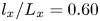 $l_x/L_x=0.60$ is obtained at the end of the self-similar region at
 $M_c=1.8$, and it is nearly 3 times larger than the largest value in the previous numerical studies by Pantano & Sarkar (Reference Pantano and Sarkar2002) and Vadrot, Giauque & Corre (Reference Vadrot, Giauque and Corre2021), and comparable to that by Pirozzoli et al. (Reference Pirozzoli, Bernardini, Marié and Grasso2015). The size of the computational domain is twice as large than those in previous numerical simulations (Pantano & Sarkar Reference Pantano and Sarkar2002; Arun et al. Reference Arun, Sameen, Srinivasan and Girimaji2019; Vadrot, Giauque & Corre Reference Vadrot, Giauque and Corre2020; Matsuno & Lele Reference Matsuno and Lele2021). Further analysis in § 4 shows that the integral length scales
 $l_x$ and
 $l_z$ are sufficiently small compared with the length of the computational domain, ensuring that the self-similar growth of large-scale structures is not confined. In order to enhance the statistical convergence, the horizontal averaging is complemented with an ensemble average over five independent runs with different initial conditions for each convective Mach number. Self-similar quantities are also time-averaged over the self-similar period.
3. Validation and general statistics
The purpose of this section is to validate our simulation by comparing present results against various previous experimental and numerical works in the literature. It is generally accepted that, after an initial transition period, the temporal mixing layer has a self-similar evolution characterised by a linear growth of momentum thickness. The selection of an appropriate self-similar range is a quite complex task because an exact self-similarity is difficult to achieve and there is no precise criteria to characterise this self-similar period. We determine the self-similar period by analysing the collapse of profiles of the mean velocity and the profiles of the Reynolds stresses, and further confirm it by computing the time evolution of the integrated transfer terms of TKE, as shown in § 4.3. The resulting time duration of the self-similar regime is indicated by intersecting vertical tick marks in figure 2(c) and reported in table 1.
Comparison of mean streamwise velocity  $\bar {u}/\Delta U$ in similarity coordinates (a)
 $y/\delta _{\theta }$ and (b)
 $y/\delta _{\omega }$. (c) Time evolution of normalised momentum thickness for different
 $M_c$, and the vertical line segments mark the self-similar time periods. (d) Comparison of linear growth rates at different
 $M_c$ with different numerical and experimental results.

Figures 2(a) and 2(b) show the mean streamwise velocity profile in similarity coordinates  $y/\delta _{\theta }$ and
 $y/\delta _{\omega }$, respectively. Compared with several previous results (Spencer & Jones Reference Spencer and Jones1971; Bell & Mehta Reference Bell and Mehta1990; Pantano & Sarkar Reference Pantano and Sarkar2002; Vaghefi et al. Reference Vaghefi, Nik, Pisciuneri and Madnia2013; Buchta & Freund Reference Buchta and Freund2017; Sharan, Matheou & Dimotakis Reference Sharan, Matheou and Dimotakis2019), very good agreement is obtained. We find that the mean streamwise velocity profiles at different convective Mach numbers collapse very well when plotted against
 $y/\delta _{\omega }$. The time evolution of the momentum thickness, normalised by its initial value (
 $\delta _\theta ^0$), is shown in figure 2(c) for different
 $M_c$. It is observed that as the convective Mach number increases, the growth rates of both transitional and self-similar regimes decrease dramatically, leading to a longer transitional time, which is consistent with previous numerical results by Pantano & Sarkar (Reference Pantano and Sarkar2002) and Vaghefi et al. (Reference Vaghefi, Nik, Pisciuneri and Madnia2013). The normalised self-similar growth rates are shown in figure 2(d), where
 $\dot {\delta }_{inc}$ is the growth rate of the quasi-incompressible case
 $M_c=0.2$ in our simulations. For comparison, the figure also shows available numerical (Pantano & Sarkar Reference Pantano and Sarkar2002; Hadjadj, Yee & Sjögreen Reference Hadjadj, Yee and Sjögreen2012; Vaghefi et al. Reference Vaghefi, Nik, Pisciuneri and Madnia2013; Buchta & Freund Reference Buchta and Freund2017) and experimental (Chinzei et al. Reference Chinzei, Masuya, Komuro, Murakami and Kudou1986; Papamoschou & Roshko Reference Papamoschou and Roshko1988; Samimy & Elliott Reference Samimy and Elliott1990; Goebel & Dutton Reference Goebel and Dutton1991; Debisschop, Chambers & Bonnet Reference Debisschop, Chambers and Bonnet1994) results in the literature.
The components of the normalised Reynolds stress are compared with previous works in figure 3 for the case M02. All variables are time-averaged over the self-similar region in similarity coordinates. It can be seen that the shape of the profiles and the peak value of Reynolds stresses are generally in good agreement with published results. For further validation of our DNS results, the dominant terms in the TKE transport equation (2.10), namely production, dissipation and transport terms, are compared with the previous results in figure 4 for cases M02, M08 and M18. These validations indicate that the current DNS provides an accurate representation of the compressible mixing layer during the self-similar stage.
Comparison of normalised components of the Reynolds stress for case M02: (a)  $\sqrt {{\mathsf{R}}_{11}}/\Delta U$, (b)
 $\sqrt {{\mathsf{R}}_{22}}/\Delta U$, (c)
 $\sqrt {{\mathsf{R}}_{33}}/\Delta U$ and (d)
 $\sqrt {-{\mathsf{R}}_{12}}/\Delta U$. The symbols denote experimental results for incompressible shear layers, and the curves represent numerical results. The legend is the same for all plots.

TKE transport equation terms in (2.10):  $\bar {P}$ (green),
 $\bar {\epsilon }$ (red) and
 $\bar {T}$ (blue) for cases (a) M02, (b) M08 and (c) M18. The budget terms are normalised by
 $\Delta U^3/\delta _\theta$. The solid lines correspond to the present DNS. The dashed lines, open and filled symbols represent the results of Rogers & Moser (Reference Rogers and Moser1994), Pantano & Sarkar (Reference Pantano and Sarkar2002) and Vaghefi (Reference Vaghefi2014), respectively.

4. Numerical results
4.1. Local compressibility
For compressible flow, the normalised velocity divergence serves as an excellent indicator of the local compressibility. To obtain an impression of the changes in the local compressibility of the mixing layer induced by convective Mach number, instantaneous fields of the normalised velocity divergence  $\varTheta \delta _{\theta }/\Delta U$ in the middle
 $x$–
 $y$ plane are shown in figure 5 at two different times, together with an isoline of vorticity magnitude
 $\omega =0.01\Delta U/\delta _{\theta }^0$ selected as the nominal threshold to identify the turbulent–non-turbulent interface (TNTI) (Jahanbakhshi & Madnia Reference Jahanbakhshi and Madnia2016; Watanabe, Zhang & Nagata Reference Watanabe, Zhang and Nagata2018). The vorticity magnitude is computed by
 $\omega = \sqrt {\omega ^2_1+\omega ^2_2+\omega ^2_3}$, where
 $\omega _i$ are vorticity components. For the subsonic flow with
 $M_c=0.2$, the results are omitted here because there is no obvious region of high compression. At
 $M_c=0.8$, several shocklets can be seen outside the mixing zone at
 $\tau =250$ in the transition region, whereas no shocklets are found at
 $\tau =1000$ in the self-similar region. At
 $M_c=1.8$, the shocklets can be observed during both transition and self-similar periods, and they tend to exhibit much smaller length scales inside the mixing layer, which is consistent with previous observations (Vaghefi et al. Reference Vaghefi, Nik, Pisciuneri and Madnia2013; Buchta & Freund Reference Buchta and Freund2017).
Visualisation of normalised velocity divergence  $\varTheta \delta _{\theta }/\Delta U$ in middle
 $x$–
 $y$ plane at two different time instants: (a)
 $M_c=0.8$,
 $\tau =250$, (b)
 $M_c=0.8$,
 $\tau =1000$, (c)
 $M_c=1.8$,
 $\tau =500$ and (d)
 $M_c=1.8$,
 $\tau =1250$. The red solid lines correspond to contours of
 $\omega =0.01\Delta U/\delta _{\theta }^0$, showing the TNTI.

To the best of the authors’ knowledge, the appearance of shocklets in simulations of three-dimensional compressible mixing layers was first reported by Vreman, Kuerten & Geurts (Reference Vreman, Kuerten and Geurts1995). However, there has been no certain critical Mach number beyond which the shocklets appear. Wang, Gotoh & Watanabe (Reference Wang, Gotoh and Watanabe2017) found that the shocklets start to form when turbulent Mach number  $M_t \ge 0.6$ in solenoidally forced compressible isotropic turbulence. Chen et al. (Reference Chen, Wang, Li, Wan and Chen2018) observed shocklets at relatively smaller turbulent Mach numbers
 $M_t \ge 0.4$ in compressible homogeneous shear turbulence owing to the higher level of velocity fluctuation. In compressible mixing layers, the occurrence of shocklets has been captured when the convective Mach number is higher than 0.7 in two-dimensional simulations (Lele Reference Lele1989). For most of the three-dimensional simulations, shocklets are observed at higher convective Mach number 1.2 (Vreman et al. Reference Vreman, Kuerten and Geurts1995; Kourta & Sauvage Reference Kourta and Sauvage2002; Vaghefi Reference Vaghefi2014; Buchta & Freund Reference Buchta and Freund2017). It is noteworthy that Zhou et al. (Reference Zhou, He and Shen2012) observed shocklets in the transition region of spatially developing compressible mixing layer at lower convective Mach number
 $M_c=0.7$. They inferred that larger initial disturbance, which leads to stronger vortical structures, might contribute to the shocklet formation at this low convective Mach number.
In figure 6, we present the temporal evolutions of the centreline turbulent Mach number  $M_{t,y0}$ and the r.m.s. velocity divergence
 $\varTheta _{rms,y0}/(\Delta U/\delta _{\theta _0})$ for simulations with
 $M_c=0.2, 0.8$ and
 $1.8$. As can be seen, a significant overshoot in the centreline turbulent Mach numbers can be observed in the transitional region, as well as the centreline r.m.s. velocity divergence, indicating that the shocklet occurs more easily in this region. We find that the critical turbulent Mach number for shocklets to appear is close to
 $M_{t,y0} = 0.4$, which agrees well with that in compressible homogeneous shear turbulence (Chen et al. Reference Chen, Wang, Li, Wan and Chen2018), and the corresponding r.m.s. velocity divergence is
 $\varTheta _{rms,y0}/(\Delta U/\delta _{\theta _0}) \approx 0.2$ for the free shear flow.
Temporal evolution of the centreline (a) turbulent Mach number  $M_{t,y0}$ and (b) r.m.s. velocity divergence
 $\varTheta _{rms,y0}/(\Delta U/\delta _{\theta _0})$ at the centreplane for simulations with
 $M_c=0.2$, 0.8 and 1.8. The dashed vertical lines mark the self-similar time periods.

Figures 7(a) and 7(b) show the probability density function (PDF) of the normalised velocity divergence inside and outside the turbulent region at several time instants for convective Mach number  $M_c = 0.8$. It was shown in previous results that the PDF of velocity divergence became more skewed towards the negative value as the turbulent Mach number and Taylor Reynolds number increase, due to strong compression region associated with shocklets which occurs much more frequently than the strong expansion region (Wang et al. Reference Wang, Shi, Wang, Xiao, He and Chen2012; Vaghefi & Madnia Reference Vaghefi and Madnia2015; Chen et al. Reference Chen, Wang, Li, Wan and Chen2019). For the moderately compressible case with
 $M_c = 0.8$, the PDF of velocity divergence in the turbulent region exhibits a skewness toward the negative side only at transition period
 $\tau =250$, and then it rapidly becomes nearly symmetric. The PDF of velocity divergence outside the turbulent region is skewed toward the negative side until
 $\tau =750$ in the self-similar period, owing to the shocklets radiated from the mixing zone.
PDF of the normalised velocity divergence  $\varTheta /(\Delta U/\delta _{\theta _0})$ at five different time instants (a),(c) in the turbulent region and (b),(d) outside the turbulent region for cases at (a),(b)
 $M_c=0.8$ and (c),(d)
 $M_c=1.8$.

Figures 7(c) and 7(d) show the PDF of the normalised velocity divergence inside and outside the turbulent region at several time instants for convective Mach number  $M_c = 1.8$. As we can see, the PDFs of velocity divergence both inside and outside the turbulent region are always strongly skewed towards the negative values. At
 $\tau =2000$, the PDF of velocity divergence inside the turbulent region is in excellent agreement with the result of Vaghefi & Madnia (Reference Vaghefi and Madnia2015) which is sampled at the beginning of the self-similar evolution. The two tails of PDF become shorter as time goes on, indicating that the local compressibility continuously decreases. We also find that the two tails of PDF inside the turbulent region are always longer than that outside the turbulent region, showing stronger local compressibility in the mixing zone.
4.2. Helmholtz decomposition of velocity fields
To reveal the underlying physics in the compressible turbulence and specifically the characteristic of local compressibility, we shall employ the well-known Helmholtz decomposition (Erlebacher & Sarkar Reference Erlebacher and Sarkar1993; Samtaney et al. Reference Samtaney, Pullin and Kosović2001; Wang et al. Reference Wang, Shi, Wang, Xiao, He and Chen2012) to the velocity field
 \begin{equation} \textbf{u} = \textbf{u}_s + \textbf{u}_d, \end{equation}
where the solenoidal component  $\textbf{u}_s$ satisfies
 $\boldsymbol {\nabla } \boldsymbol {\cdot } \textbf{u}_s = 0$ and the dilatational component
 $\textbf{u}_c$ is irrotational, i.e.
 $\boldsymbol {\nabla }\times \textbf{u}_d = 0$.
The instantaneous fields of decomposed velocity in the  $x$–
 $y$ plane at
 $z=L_z/2$ are presented in figures 8 and 9 for the cases with
 $M_c=0.8$ at
 $\tau =1000$ and
 $M_c=1.8$ at
 $\tau =1700$, respectively. Note that all visualisations are selected at the middle of the self-similar region. For solenoidal velocity component, the visualisations in figures 8(a),(c),(e) and 9(a),(c),(e) show the typical features of a turbulent mixing layer, with patches of mixed fluid in the central region entraining patches of unmixed fluid from both external streams. It can be seen that the
 $u_s^{\prime \prime }$ field in the
 $x$–
 $y$ plane is characterised by elongated low- and high-speed regions, with characteristic sizes of the order of
 $\delta _\omega$. Comparing figures 8(a) and 8(c) or figures 9(a) and 9(c) reveals a strong anticorrelation between
 $u_s^{\prime \prime }$ and
 $v_s^{\prime \prime }$ events. The large-scale negative
 $u_s^{\prime \prime }$ events are characterised by regions of positive
 $v_s^{\prime \prime }$, upraising the low-speed fluid. The large-scale positive
 $u_s^{\prime \prime }$ events are accompanied by regions of negative
 $v_s^{\prime \prime }$, moving the high-speed fluid downwards. Moreover, the solenoidal velocity fields become visibly smoother at small scales for higher convective Mach number
 $M_c = 1.8$. Figures 10 and 11 show the instantaneous fields of decomposed velocity in
 $x$–
 $z$ plane at
 $y=0$ for cases with
 $M_c=0.8$ at
 $\tau =1000$ and
 $M_c=1.8$ at
 $\tau =1700$, respectively. The main characteristic of the solenoidal velocity field is consistent with that found previously in the
 $x$–
 $y$ plane. The presence of large-scale streamwise elongated streaks of
 $u_s^{\prime \prime }$ is presented more clearly in the
 $x$–
 $z$ plane visualisation, with spanwise sizes of about
 $L_z/4$ in the self-similar state. This indicates that the spanwise length of the domain is large enough for the present simulation.
Instantaneous fields of (a)  $u_s^{\prime \prime }$, (b)
 $u_d^{\prime \prime }$, (c)
 $v_s^{\prime \prime }$, (d)
 $v_d^{\prime \prime }$, (e)
 $w_s^{\prime \prime }$ and ( f)
 $w_d^{\prime \prime }$ in the central
 $x$–
 $y$ plane for case M08 at
 $\tau =1000$.

Instantaneous fields of (a)  $u_s^{\prime \prime }$, (b)
 $u_d^{\prime \prime }$, (c)
 $v_s^{\prime \prime }$, (d)
 $v_d^{\prime \prime }$, (e)
 $w_s^{\prime \prime }$ and ( f)
 $w_d^{\prime \prime }$ in the central
 $x$–
 $y$ plane for the case M18 at
 $\tau =1700$.

Instantaneous fields of (a)  $u_s^{\prime \prime }$, (b)
 $u_d^{\prime \prime }$, (c)
 $v_s^{\prime \prime }$, (d)
 $v_d^{\prime \prime }$, (e)
 $w_s^{\prime \prime }$ and ( f)
 $w_d^{\prime \prime }$ in the central
 $x$–
 $z$ plane for case M08 at
 $\tau =1000$.

Instantaneous fields of (a)  $u_s^{\prime \prime }$, (b)
 $u_d^{\prime \prime }$, (c)
 $v_s^{\prime \prime }$, (d)
 $v_d^{\prime \prime }$, (e)
 $w_s^{\prime \prime }$ and ( f)
 $w_d^{\prime \prime }$ in the central
 $x$–
 $z$ plane for case M18 at
 $\tau =1700$.

As can be seen in the right subfigures of figures 8 to 11, the increasing of convective Mach number induces different flow patterns of dilatational velocity component both in the  $x$–
 $y$ and
 $x$–
 $z$ planes. For the case with
 $M_c=0.8$, all three dilatational velocity components exhibit large block-like spatial structures. The
 $u_d^{\prime \prime }$ and
 $v_d^{\prime \prime }$ structures are aligned at oblique angles to the streamwise direction in
 $x$–
 $y$ plane, whereas the
 $w_d^{\prime \prime }$ structure is almost perpendicular. The
 $v_d^{\prime \prime }$ and
 $w_d^{\prime \prime }$ structures extend over the entire spanwise length of the domain, as shown in figures 10(d) and 10( f). These results suggest the presence of the spanwise rollers at
 $M_c=0.8$, which also can be observed in the instantaneous fields of solenoidal velocity in the
 $x$–
 $y$ plane, as shown in figures 8(a), 8(c) and 8(e).
At convective Mach number  $M_c=1.8$, all three dilatational velocity components show severe discontinuity at the position of shocklets, particularly in the non-turbulent region, as presented in figures 9(b), 9(d) and 9( f). As can be seen, the fluids on two sides of shocklets move towards the shocklets and generate a sheet-like strong compressible region, causing a strong anticorrelation between
 $u_d^{\prime \prime }$ and
 $v_d^{\prime \prime }$ events. In the middle
 $x$–
 $z$ plane, the
 $u_d^{\prime \prime }$ and
 $v_d^{\prime \prime }$ events are also anticorrelated, which becomes less apparent masked by the trivial spanwise structures of
 $u_d^{\prime \prime }$.
To have a better picture of the effect of convective Mach number on the correlation between streamwise and vertical velocity components, we present the joint PDF of the velocity components, computed inside and outside the turbulent region at an instant in the self-similar region. As shown in figure 12(a), the joint PDF of  $u_s^{\prime \prime }/u_{s,rms}^{\prime \prime }$ and
 $v_s^{\prime \prime }/v_{s,rms}^{\prime \prime }$ in the turbulent region reveals a statistical preference for points in the second and fourth quadrants, appearing as the oval contour lines. The long axis of the oval shape of PDF(
 $u_s^{\prime \prime }$,
 $v_s^{\prime \prime }$) exhibits an inclined angle with the symmetry line of the
 $u_s^{\prime \prime }$–
 $v_s^{\prime \prime }$ plane, indicating the component anisotropy of solenoidal velocity components. This oval shape of the PDF(
 $u_s^{\prime \prime }$,
 $v_s^{\prime \prime }$) is consistent well with that in incompressible homogeneous shear flow (Adrian & Moin Reference Adrian and Moin1988) and different from the results in the wall-bounded turbulent flow where axisymmetric shapes are usually observed (Wallace Reference Wallace2016; Yu, Xu & Pirozzoli Reference Yu, Xu and Pirozzoli2019; Xu et al. Reference Xu, Wang, Wan, Yu, Li and Chen2021a). PDF(
 $u_s^{\prime \prime }$,
 $v_s^{\prime \prime }$) in the non-turbulent region decays rapidly, illustrating the solenoidal velocity components are insignificant here, as can be seen from figure 12(b).
Joint PDF of (a),(b)  $u_s^{\prime \prime }/u_{s,rms}^{\prime \prime }$ and
 $v_s^{\prime \prime }/v_{s,rms}^{\prime \prime }$ and (c),(d)
 $u_d^{\prime \prime }/u_{d,rms}^{\prime \prime }$ and
 $v_d^{\prime \prime }/v_{d,rms}^{\prime \prime }$ for case with
 $M_c=0.8$ at
 $\tau =1000$ and
 $M_c=1.8$ at
 $\tau =1250$: (a),(c) in the turbulent region and (b),(d) in the non-turbulent region. The thick dashed auxiliary line indicates the long axis of the oval shape. The thin dashed-dotted line represents the symmetry line of the
 $u_s^{\prime \prime }$–
 $v_s^{\prime \prime }$ plane. The contour levels 0.001, 0.01 and 0.1 are shown.

The joint PDFs of  $u_d^{\prime \prime }/u_{d,rms}^{\prime \prime }$ and
 $v_d^{\prime \prime }/v_{d,rms}^{\prime \prime }$ are plotted in figures 12(c) and 12(d). In the turbulent region, we find that there is no significant correlation between
 $u_d^{\prime \prime }$ and
 $v_d^{\prime \prime }$ for
 $M_c=0.8$, whereas PDF(
 $u_d^{\prime \prime }$,
 $v_d^{\prime \prime }$) also has a statistical preference in the second and fourth quadrants for
 $M_c=1.8$, showing an oval shape similar to that of PDF(
 $u_s^{\prime \prime }$,
 $v_s^{\prime \prime }$). In the non-turbulent region, both for
 $M_c=0.8$ and
 $M_c=1.8$, PDF(
 $u_d^{\prime \prime }$,
 $v_d^{\prime \prime }$) has the inclined oval pattern, which is elongated in the
 $u_d^{\prime \prime }$ direction for
 $M_c=1.8$ compared with that in the turbulent region. Actually, we find that, as the development of turbulent flow, the inclination angle of the oval shape of the PDF(
 $u_d^{\prime \prime }$,
 $v_d^{\prime \prime }$) for
 $M_c=0.8$ in non-turbulent region increases monotonically from
 $10^\circ$ at
 $\tau =200$ to nearly
 $30^\circ$ at
 $\tau =1000$. Only the results at
 $\tau =1000$ is illustrated here in figure 12(d) for brevity.
It is worth noting that the statistical preference in the second and fourth quadrants of PDF( $u_s^{\prime \prime }$,
 $v_s^{\prime \prime }$) and PDF(
 $u_d^{\prime \prime }$,
 $v_d^{\prime \prime }$) corresponds to totally different physical processes. The former is related to the mixing between the two streams, demonstrated in the left subfigures of figures 8–11, resembling the sweep and ejection events in wall-bounded turbulent shear flow, and the latter is due to the induction of strong compression or expansion motions, seen from the right subfigures of figures 8–11.
On the basis of Helmholtz decomposition of velocity, the Reynolds stress  ${\mathsf{R}}_{ij}$ can be decomposed into
 \begin{equation} {\mathsf{R}}_{ij} = \overline{\rho u_i^{\prime\prime}u_j^{\prime\prime}} = \overline{\rho u_{s,i}^{\prime\prime}u_{s,j}^{\prime\prime}}+ \overline{\rho u_{d,i}^{\prime\prime}u_{d,j}^{\prime\prime}}+ \overline{\rho u_{s,i}^{\prime\prime}u_{d,j}^{\prime\prime}}+ \overline{\rho u_{d,i}^{\prime\prime}u_{s,j}^{\prime\prime}}. \end{equation}
However, it is found that in the turbulent region the magnitudes of the last three terms on the right-hand side of (4.2) are several orders of magnitude smaller than the first term, even for the highest convective Mach number  $M_c=1.8$. Then we take Reynolds shear stress
 ${\mathsf{R}}_{12}=\overline {\rho u^{\prime \prime }v^{\prime \prime }}$ for example to show the effect of compressibility, and the Helmholtz decomposition of Reynolds normal stresses
 ${\mathsf{R}}_{11}$,
 ${\mathsf{R}}_{22}$ and
 ${\mathsf{R}}_{33}$ can be found in Appendix B. The statistical preference in the second and fourth quadrants of PDF(
 $u_s^{\prime \prime }$,
 $v_s^{\prime \prime }$) and PDF(
 $u_d^{\prime \prime }$,
 $v_d^{\prime \prime }$) above shows that both solenoidal and dilatational velocity have a contribution to the negative values of the Reynolds shear stress. Figure 13 provides the Reynolds shear stress and its decomposed components for cases with
 $M_c=0.8$ and
 $M_c=1.8$. We can see that
 ${\mathsf{R}}_{ij}$ and
 $\overline {\rho u_{s}^{\prime \prime }v_{s}^{\prime \prime }}$ overlap almost perfectly with each other for both
 $M_c=0.8$ and
 $M_c=1.8$, indicating the dominant role of the solenoidal velocity field. For
 $M_c=0.8$,
 $\overline {\rho u_{s}^{\prime \prime }v_{d}^{\prime \prime }}$ is positive with a peak value at
 $y=0$ and is significantly greater than the negligible two terms
 $\overline {\rho u_{d}^{\prime \prime }v_{d}^{\prime \prime }}$ and
 $\overline {\rho u_{d}^{\prime \prime }v_{s}^{\prime \prime }}$. For
 $M_c=1.8$, the values of three dilatation-related terms are on the same order. As the convective Mach number increases, the magnitudes of three dilatation-related terms become larger, demonstrating the effect of compressibility. It is interesting to note that for
 $M_c=1.8$,
 $\overline {\rho u_{d}^{\prime \prime }v_{d}^{\prime \prime }}$ has two peak values at
 $y/\delta _\omega \approx \pm 0.5$ and becomes larger than
 $\overline {\rho u_{s}^{\prime \prime }v_{s}^{\prime \prime }}$ in the non-turbulent region, which is probably due to the induction of the shocklets frequently formed near the TNTI, consistent with the analysis of figure 9.
The Reynolds shear stress and its decomposed components for cases with (a)  $M_c=0.8$ and (b)
 $M_c=1.8$. The legend is the same for both plots.

4.3. Integrated TKE transport
The physical mechanism of the suppression of layer growth rate due to compressibility is further examined by analysing the time evolution of integrated TKE transport. The terms in conservative form disappear after integration, hence the equation of the  $y$-integrated TKE becomes (Vreman et al. Reference Vreman, Sandham and Luo1996; Attili & Bisetti Reference Attili and Bisetti2012)
 \begin{equation} \frac{\partial \hat{K}}{\partial t} = \hat{P} + \hat{\epsilon} + \hat{\varPhi} + \hat{\varSigma}, \end{equation}
where
 \begin{equation} \hat{K} = \int_{{-}L_y/2}^{L_y/2}\frac{1}{2}\overline{\rho u_i^{\prime\prime}u_i^{\prime\prime}}\,{{\rm d} y}, \end{equation}
is total TKE, and the integrated transport terms  $\hat {P}$,
 $\hat {\epsilon }$,
 $\hat {\varPhi }$ and
 $\hat {\varSigma }$ are
 $$\begin{gather} \hat{P}={-} \int_{{-}L_y/2}^{L_y/2}R_{ik}\frac{\partial \tilde{u}_i}{\partial x_k}\,{{\rm d} y}, \end{gather}$$
 $$\begin{gather}\hat{\epsilon}={-}\int_{{-}L_y/2}^{L_y/2}\frac{1}{Re}\overline{\sigma^\prime_{ik}\frac{\partial u^{\prime\prime}_i}{\partial x_k}}\,{{\rm d} y}, \end{gather}$$
 $$\begin{gather}\hat{\varPhi}= \int_{{-}L_y/2}^{L_y/2}\overline{p^\prime\frac{\partial u^{\prime\prime}_i}{\partial x_i}}\,{{\rm d} y}, \end{gather}$$
 $$\begin{gather}\hat{\varSigma}= \int_{{-}L_y/2}^{L_y/2}\overline{u_i^{\prime\prime}}\left(\frac{1}{Re}\frac{\partial\bar{\sigma}_{ik}}{\partial x_k} - \frac{\partial \bar{p}}{\partial x_i}\right){{\rm d} y}. \end{gather}$$
The magnitude of the integrated mass flux coupling term is still negligible. The transport equations of the integrated TKE components  $\hat {K}_i$ and the Reynolds shear stress
 $\hat {R}_{12}$ can be obtained similarly, which are omitted here for brevity.
Figure 14 displays the time evolution of the normalised  $y$-integrated TKE
 $\hat {K}/\Delta U^2$, its three components
 $\hat {K}_i/\Delta U^2$ and the Reynolds shear stress
 $\hat {R}_{12}/\Delta U^2$ at
 $M_c=0.2$,
 $0.8$ and
 $1.8$. We can see that the integrated TKE and Reynolds shear stress grow linearly after a rapid growing transition region with a slight overshoot between two regions only at
 $M_c=0.8$. Because of the anisotropic nature of free shear flows, it is generally observed that the components of integrated TKE satisfy the relationship
 $\hat {K}_1 > \hat {K}_3 > \hat {K}_2$ in the self-similar region. It is interesting for
 $M_c=0.2$ that the vertical component
 $\hat {K}_2$ of the TKE is larger than the spanwise component
 $\hat {K}_3$ in transition region
 $\tau <150$, and undergoes an accelerating growth resulting in
 $\hat {K}_2 > \hat {K}_3$ again beyond the self-similar region
 $\tau >750$, as shown in figure 14(a). This behaviour is consistent with a previous numerical study of a spatially developing incompressible mixing layer by Attili & Bisetti (Reference Attili and Bisetti2012). We observe that the rapid growth of
 $\hat {K}_2$ in the late stages of development at
 $M_c=0.2$ is the characteristic of the larger spanwise rollers generated by the Kelvin–Helmholtz instability, which is in agreement with previous results by Rogers & Moser (Reference Rogers and Moser1994).
Time evolution of  $\hat {K}/\Delta U^2$,
 $\hat {K}_i/\Delta U^2$,
 $0.5\hat {R}_{12}/\Delta U^2$ at (a)
 $M_c=0.2$, (b)
 $M_c=0.8$ and (c)
 $M_c=1.8$. The legend is the same for all plots. The dashed vertical lines mark the self-similar time periods.

Figure 15 displays the time evolution of the normalised  $y$-integrated production
 $\hat {P}/\Delta U^3$, dissipation
 $\hat {\epsilon }/\Delta U^3$ and pressure–strain
 $\hat {\varPhi }/\Delta U^3$ in the equation of
 $\hat {K}$ at
 $M_c=0.2$,
 $M_c=0.8$ and
 $M_c=1.8$. Here, the integrated mass flux coupling and transport terms have been neglected because their magnitude is very small, even in the large
 $M_c$ case. At
 $M_c=0.2$, the asymptotic behaviour of
 $\hat {P}/\Delta U^3$ and
 $\hat {\epsilon }/\Delta U^3$ is in good agreement with the previous numerical results by Attili & Bisetti (Reference Attili and Bisetti2012) in a spatially evolving incompressible mixing layer, as compared in figure 15(b) where the abscissa is a local Reynolds number
 $Re_\omega = \rho _\infty \Delta U \delta _\omega /\mu _\infty$, which allows a direct comparison between the spatially and temporally evolving mixing layers. As convective Mach number increases, both magnitudes of the integrated production and dissipation become smaller, whereas the integrated pressure–strain term slightly increases only in the transition region. We can see that the integrated pressure–strain term is always much smaller than the other two terms, indicating that the net contribution of pressure dilatation to the kinetic energy transfer is negligibly small. This is consistent with previous studies on compressible turbulence (Wang et al. Reference Wang, Wan, Chen and Chen2018, Reference Wang, Wang, Li and Chen2021). In the transition region,
 $\hat {P}/\Delta U^3$ grows linearly for all three convective Mach numbers. In contrast,
 $\hat {\epsilon }/\Delta U^3$ grows linearly only at
 $M_c=1.8$ and it satisfies
 $\hat {\epsilon }/\Delta U^3 \propto -\tau ^2$ at
 $M_c=0.2$ and
 $M_c=0.8$. An overshoot in the integrated production and dissipation occurs near the end of the transition region, and then the overshoot decays and becomes nearly a constant in the self-similar region. We also observe that the dissipation overshoot clearly lags behind the production overshoot. The ratio between the corresponding time of the dissipation overshoot
 $\tau _\epsilon$ and the production overshoot
 $\tau _P$ is defined to measure the lag level between them. The values for
 $\tau _\epsilon /\tau _P$ are 1.8, 1.5 and 1.2 at
 $M_c=0.2$,
 $M_c=0.8$ and
 $M_c=1.8$, respectively. This result indicates that the dissipation starts to effectively balance the production earlier for larger convective Mach number, and partly reveals some reasons for reduction of growth rate with increased convective Mach number in the transition region.
Time evolution of  $\hat {P}/\Delta U^3$,
 $\hat {\epsilon }/\Delta U^3$,
 $\hat {\varPhi }/\Delta U^3$ at (a),(b)
 $M_c=0.2$, (c)
 $M_c=0.8$ and (d)
 $M_c=1.8$. The legend is the same for (a), (c) and (d). The black solid lines correspond to
 $\hat {\epsilon }/\Delta U^3 \propto -\tau ^2$. The dashed vertical lines mark the self-similar time periods.

In order to better understand the effect of compressibility, we plot the time evolution of transport terms for  $\hat {K}_i$ in figure 16. In all cases, we can see that the production terms associated with
 $\hat {K}_2$ and
 $\hat {K}_3$, namely
 $\hat {P}_2$ and
 $\hat {P}_3$, are negligible concerning the
 $\hat {K}_1$ production
 $\hat {P}_1$. As is well known, on average, the pressure–strain correlation components
 $\hat {\varPhi }_i$ redistribute energy from
 $\hat {K}_1$ to the other components
 $\hat {K}_2$ and
 $\hat {K}_3$. Figure 16(a) shows that
 $\hat {\varPhi }_2 > \hat {\varPhi }_3$ for
 $\tau <100$ and
 $\tau >700$, leading to the preferential transfer of energy into the vertical velocity fluctuation, as shown in figure 14(a). It is interesting to note that all pressure–strain correlation components
 $\hat {\varPhi }_i$ and production almost reach their peak values at the same time for all three convective Mach numbers.
Time evolution of  $\hat {P}_i/\Delta U^3$,
 $\hat {\epsilon }_i/\Delta U^3$,
 $\hat {\varPhi }_i/\Delta U^3$ at (a)
 $M_c=0.2$, (b)
 $M_c=0.8$ and (c)
 $M_c=1.8$. The legend is the same for all plots. The black solid lines correspond to
 $\hat {\epsilon }_i/\Delta U^3 \propto -\tau ^2$.

For the case with  $M_c=0.2$, the three components of viscous dissipation
 $\hat {\epsilon }_i$ always overlap perfectly with each other, as shown in figure 16(a), suggesting local isotropy of the flow at small scales. As the convective Mach number increases, the viscous dissipation occurs more anisotropically and is dominated by the streamwise component
 $\hat {\epsilon }_1$ in the transition region. As is clearly presented in figure 16(c) for
 $M_c=1.8$, the magnitude of streamwise component
 $\hat {\epsilon }_1$ is found to be even larger than
 $\hat {\varPhi }_1$, whereas the
 $\hat {\epsilon }_2$ and
 $\hat {\epsilon }_3$ components are still proportional to
 $-\tau ^2$, resulting in linear growth of the total viscous dissipation
 $\hat {\epsilon }$ in figure 15(d). We depict the PDF of three instantaneous viscous dissipation components
 ${\epsilon }_i/\Delta U^3$ at
 $\tau =250$ in figure 17 for the convective Mach number
 $M_c = 0.2$ and
 $1.8$, where
 ${\epsilon }_i$ is defined as (avoiding summation convention)
 \begin{equation} \epsilon_i={-}\frac{1}{Re}{\sigma^\prime_{ik}\frac{\partial u^{\prime\prime}_i}{\partial x_k}}. \end{equation}
The PDFs of  ${\epsilon }_i/\Delta U^3$ always collapse into the same curve for
 $M_c = 0.2$. At convective Mach number
 $M_c = 1.8$, we observe that the left tail of PDF of
 ${\epsilon }_1/\Delta U^3$ is much longer than that of
 ${\epsilon }_2/\Delta U^3$ and
 ${\epsilon }_3/\Delta U^3$, suggesting that stronger events of viscous dissipation occur in the transport of
 $\hat {K}_1$ during the transition region. This is further studied from aspect of vortical structures in § 4.4.
PDF of viscous dissipation components  ${\epsilon }_i/\Delta U^3$ at
 $\tau =250$ for cases with (a)
 $M_c=0.2$ and (b
 $M_c=1.8$.

We also plot the time evolution of transport terms for  $\hat {R}_{12}$ in figure 18. For all cases, we can see that the transfer of the Reynolds shear stress is dominated by the pressure–strain term
 $\hat {\varPhi }_{12}$ and production term
 $\hat {P}_{12}$ with peaks occurring at nearly the same time with the production
 $\hat {P}$. The viscous dissipation
 $\hat {\epsilon }_{12}$ is negligibly small and increases slightly as the convective Mach number increases.
Time evolution of  $\hat {P}_{12}/\Delta U^3$,
 $\hat {\epsilon }_{12}/\Delta U^3$,
 $\hat {\varPhi }_{12}/\Delta U^3$ at (a)
 $M_c=0.2$, (b)
 $M_c=0.8$ and (c)
 $M_c=1.8$. The legend is the same for all plots. The dashed vertical lines mark the self-similar time periods.

4.4. Turbulence structure and length scale
As already mentioned, the contribution of dilatational component to overall Reynolds stress is quite limited. We therefore believe that the transportation of TKE is dominated by the solenoidal velocity field which is characterised by small-scale vortical structures and energetic large-scale velocity structures. According to Kolmogorov's turbulence theory (Kolmogorov Reference Kolmogorov1941), the characteristic length scale of the smallest eddies is given by the Kolmogorov length scale  $\eta$ where most of the kinetic energy is dissipated by viscosity. Figure 19(a) shows the temporal evolution of the normalised centreline Kolmogorov length scale
 $\eta _{y0}/\Delta x$ for cases with convective Mach numbers
 $M_c = 0.2$, 0.8 and 1.8. We observe that
 $\eta _{y0}/\Delta x$ at
 $y=0$ reaches a minimum value during the transition region and then gradually increases as the development of turbulent flow. As the convective Mach number increases, the centreline Kolmogorov length scale
 $\eta _{y0}/\Delta x$ at
 $M_c = 1.8$ becomes twice as large as that at
 $M_c = 0.2$. From figure 19(b), it can be seen that the
 $\eta /\Delta x$ extracted in the self-similar region is approximately constant inside the turbulent mixing region, which is consistent with the previous results of compressible turbulent mixing layer by Vaghefi & Madnia (Reference Vaghefi and Madnia2015) and incompressible planar jet by Watanabe et al. (Reference Watanabe, Zhang and Nagata2018). Outside the mixing layer,
 $\eta /\Delta x$ decreases as the convective Mach number increases, due to the fluctuations induced by the shocklets here.
(a) Time evolution of the centreline Kolmogorov length scale  $\eta _{y0}/\Delta x$ and (b) mean profile of
 $\eta /\Delta x$ at
 $M_c=0.2, 0.8$ and
 $1.8$. The dashed vertical lines mark the self-similar time periods in (a).

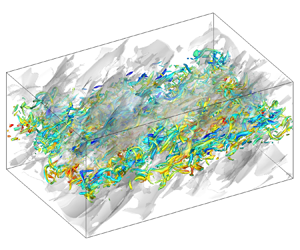
In figure 20, we compare the visualisations of small-scale vortical structures in transition region at  $M_c = 0.2$ and
 $1.8$, where the structures are displayed by the iso-surfaces of the second invariant of the instantaneous velocity gradient tensor
 $\boldsymbol{\mathsf{Q}}$. At lower convective Mach number
 $M_c = 0.2$, the vortices are highly three-dimensional, with their diameter of the same order of the Kolmogorov scale. There are plentiful shapes of small-scale vortices, including hairpin vortices, rib vortices and complex helical vortices, giving rise to much random orientation of vortical structures. In contrast, the flow field is dominated by more regular and smooth streamwise elongated vortices at
 $M_c = 1.8$ and
 $\tau =250$. This phenomenon is consistent with previous studies of small-scale vortical structures in compressible mixing layer, where it is generally believed that the vortical structures are more aligned in the streamwise direction at higher
 $M_c$, particularly in the transition region (Balaras et al. Reference Balaras, Piomelli and Wallace2001; Fathali et al. Reference Fathali, Meyers, Rubio, Smirnov and Baelmans2008; Arun et al. Reference Arun, Sameen, Srinivasan and Girimaji2019; Li et al. Reference Li, Peyvan, Ghiasi, Komperda and Mashayek2021).
Small-scale vortical structures are visualised by the iso-surfaces of the second invariant  $Q$ of the velocity gradient tensor and coloured based on local values of
 $u^{\prime \prime }$: (a)
 $Q=20$,
 $\tau =125$ and
 $M_c=0.2$; (b)
 $Q=2$,
 $\tau =250$ and
 $M_c=1.8$.

The effects of the small-scale vortical structures on the anisotropy of viscous dissipation are further investigated by scrutinising flow variables in the  $y$–
 $z$ planes, as shown in figure 21. In these
 $y$–
 $z$ slices at
 $x=0.5L_x$, the black solid lines represent the iso-lines of viscous dissipation, whereas the contours show the velocity fluctuation. For case M02, the distribution of streamwise viscous dissipation
 ${\epsilon _1}$ is chaotic and fragmental, as shown in figure 21(a). Here
 ${\epsilon _2}$ and
 ${\epsilon _3}$ are not shown because they resemble
 ${\epsilon _1}$. For case M18, the mixing region is packed with mushroom-like structures of positive and negative streamwise velocity fluctuations, with strong streamwise viscous dissipation regions wrapping around them. Comparing figures 21(b) and 21(c), the lift-up of low-speed fluid and the drop-down of high-speed fluid are clearly presented. The prominent mushroom-like structures are created by the interaction of a pair of streamwise counter-rotating vortices, as presented in a enlarged view in figure 21(e), with the vectors showing the velocity fluctuations in the vertical
 $v^{\prime \prime }$ and spanwise
 $w^{\prime \prime }$ directions. This is similar to several previous studies on flat-plate boundary layers (Strand & Goldstein Reference Strand and Goldstein2011; Buffat et al. Reference Buffat, Penven, Cadiou and Montagnier2014; Zhao & Sandberg Reference Zhao and Sandberg2020). From figures 21(c) and 21(d), we can see that the iso-lines of
 ${\epsilon _2=0.005}$ and
 ${\epsilon _3=0.005}$ are more sparse, with smaller length scales in the
 $y$–
 $z$ plane, as compared with the iso-lines of
 ${\epsilon _1=0.01}$, revealing that the viscous dissipation of
 ${K}_2$ and
 ${K}_3$ is much weaker than that of
 ${K}_1$ for
 $M_c=1.8$ in the transition region, which confirms the results in figure 16.
Contours of instantaneous velocity fluctuations  $u_i^{\prime \prime }$ along with stronger events of viscous dissipation indicated by black solid lines: (a)
 ${\epsilon _1}/\Delta U^3=0.03$,
 $-0.3< u^{\prime \prime }<0.3$ at
 $M_c=0.2$ and
 $\tau =125$; (b)
 ${\epsilon _1}/\Delta U^3=0.01$,
 $-0.3< u^{\prime \prime }<0.3$, (c)
 ${\epsilon _2}/\Delta U^3=0.005$,
 $-0.2< v^{\prime \prime }<0.2$, and (d)
 ${\epsilon _3}/\Delta U^3=0.005$,
 $-0.2< w^{\prime \prime }<0.2$ at
 $M_c=1.8$ and
 $\tau =250$. (e) Enlarged view of the region in red-lined rectangular box in plot (b), showing the velocity vectors of
 $v$ and
 $w$.

We are now going to focus on the large-scale flow structures of the mixing shear layer. Figures 22 and 23 show the instantaneous fields of the streamwise velocity  $u^{\prime \prime }$ and density fluctuations
 $\rho ^{\prime }$ in the horizontal plane at the centre of the shear layer (
 $y = 0$) at different time instants for cases M02 and M18, respectively. For the nearly incompressible case with
 $M_c=0.2$, the density fields exhibit a typical pattern of spanwise Kelvin–Helmholtz rollers that merge and eventually fill up the whole computational domain, which is similar to the situation reported in incompressible (Rogers & Moser Reference Rogers and Moser1994; Balaras et al. Reference Balaras, Piomelli and Wallace2001) and weakly compressible (Mungal Reference Mungal1995; Pirozzoli et al. Reference Pirozzoli, Bernardini, Marié and Grasso2015) mixing shear layers. The streamwise elongated large-scale structures of
 $u^{\prime \prime }$ with an imposed low-frequency spanwise meander can also be observed in the transition region at
 $\tau =375$. At late time
 $\tau =750$, we can see that the high-speed regions tend to propagate abreast along the spanwise direction. For the strongly compressible case with
 $M_c=1.8$, no clear hints of spanwise rollers can be observed both in the fields of the streamwise velocity
 $u^{\prime \prime }$ and density fluctuations
 $\rho ^{\prime }$. Although large-scale low- and high-speed regions form at an early time of
 $\tau =125$, they are highly elongated in the streamwise direction and more slender in the spanwise direction.
Instantaneous fields of (a),(c),(e)  $u^{\prime \prime }$ and (b),(d),(f)
 $\rho^{\prime}$ in the central
 $x$–
 $z$ plane for case M02: (a),(b)
 $\tau =100$; (c),(d)
 $\tau =375$; and (e),(f)
 $\tau =750$.

Instantaneous fields of (a),(c),(e)  $u^{\prime \prime }$ and (b),(d),(f)
 $\rho ^{\prime }$ in the central
 $x$–
 $z$ plane for case M18: (a),(b)
 $\tau =125$; (c),(d)
 $\tau =500$; and (e),(f)
 $\tau =2000$.

To quantify the features of streamwise elongated large-scale structures in the mixing shear layer, the two-point correlation  $R_{uu}$ (defined in (2.19)) at three different time instants in the self-similar region is shown in figure 24 at
 $M_c=0.2$ and 1.8. Ten contour levels ranging from 0.1 to 1 with increments of 0.1 are shown and each direction is normalised by the local vorticity thickness
 $\delta _\omega$. The undulation of the lower
 $R_{uu}$ level is caused by the decreasing sample size away from the origin. We find that the three sets of contours (at three different time instants) in the self-similar region show very good collapse when scaled by vorticity thickness
 $\delta _\omega$ for both
 $M_c=0.2$ and
 $1.8$, which confirms that the self-similar state of the mixing layer is dominated by large-scale structures (Vreman et al. Reference Vreman, Sandham and Luo1996; Pantano & Sarkar Reference Pantano and Sarkar2002). In figures 24(a) and 24(b), the correlation decays to a value of 0.1 at a distance larger than
 $\delta _\omega$, which indicates that there is significant streamwise elongated spatial coherence. The fusiform-like correlation contours are inclined with respect to the local streamwise direction with an inclination angle decreasing from
 $18^\circ$ at
 $M_c=0.2$ to
 $12^\circ$ at
 $M_c=1.8$, which is similar to the experimental results reported by Messersmith & Dutton (Reference Messersmith and Dutton1996) and Kim, Elliott & Dutton (Reference Kim, Elliott and Dutton2020). Figures 24(c),(d) and 24(e),(f) show
 $R_{uu}$ in the
 $x$–
 $z$ and
 $y$–
 $z$ planes, respectively. We find that the correlation contours are compact in spanwise direction and moderately elongated in the vertical direction, indicating a relatively small spanwise length scale.
Two-point correlations of the streamwise velocity fluctuation  $u^{\prime \prime }$ in the (a),(b)
 $x$–
 $y$, (c),(d)
 $x$–
 $z$ and (e),(f)
 $y$–
 $z$ planes at three different time instants: (a),(c),(e)
 $M_c=0.2$ and (b),(d),(f)
 $M_c=1.8$. The contour levels range from 0.1 to 1 with increments of 0.1.

In general, the streamwise and spanwise length scales of large-scale structures are extracted from the two-point correlation functions of the streamwise velocity fluctuations with a nominal threshold. A higher threshold leads to smaller and more stable coherence length (Ganapathisubramani et al. Reference Ganapathisubramani, Hutchins, Hambleton, Longmire and Marusic2005; Sillero, Jiménez & Moser Reference Sillero, Jiménez and Moser2014). Here, it is found that the threshold strongly influences the streamwise correlation length, so it is difficult to determine the compressibility effect on the length scale. For example, when we chose a larger value of the threshold,  $R_{uu} \ge 0.3$, the streamwise length scale was found to be larger at
 $M_c=0.2$, in contrast to the situation of the threshold value 0.1. The compressibility effect on the length scale of large-scale structures is further investigated by inspecting the integral length scales, as shown in figure 25. We can see that the normalised integral length scales
 $l_x/\delta _\omega$ and
 $l_x/\delta _\omega$ rapidly decrease in the transition region from a very large initial value, then followed by a nearly constant length scale until the end of the simulation, confirming again the self-similarity of large-scale structures. This observation indicates that the current computational domain is large enough to solve the large-scale turbulence. Otherwise, the growth of large-scale structures would be restricted resulting in the decrease of integral length scale (Vreman et al. Reference Vreman, Sandham and Luo1996; Vadrot et al. Reference Vadrot, Giauque and Corre2021). In the self-similar region, the streamwise length scale
 $l_x/\delta _\omega$ increases significantly with the convective Mach number, indicating that the large-scale structures of
 $R_{uu}$ became increasingly elongated in the streamwise direction. As the convective Mach number increases, the spanwise integral length scale is almost unchanged with
 $l_z/\delta _\omega \approx 0.3$, whereas a clear decrease of the spanwise size of large scale structures can be found in figure 24. We also find that the spanwise integral length scale agrees very well with the previous study of a compressible spatially developing mixing layer (Pirozzoli et al. Reference Pirozzoli, Bernardini, Marié and Grasso2015).
Evolutions of the normalised integral length scales in the streamwise direction  $l_x/\delta _\omega$ and in the spanwise direction
 $l_z/\delta _\omega$ for (a)
 $M_c=0.2$ and (b)
 $M_c=1.8$. The dashed vertical lines mark the self-similar time periods.

In the stratified shear layer, the turbulent structures and flow dynamics have been found to resemble those in wall turbulence (Watanabe et al. Reference Watanabe, Riley, Nagata, Matsuda and Onishi2019; Watanabe & Nagata Reference Watanabe and Nagata2021). The universality of the elongated large-scale structures can be examined in compressible temporally evolving mixing layers and turbulent boundary layers. The spanwise integral length scale is comparable to that observed in the logarithmic region of turbulent boundary layers (Pirozzoli & Bernardini Reference Pirozzoli and Bernardini2011; Pirozzoli Reference Pirozzoli2012), where  $l_z/\delta \approx 0.2\unicode{x2013}0.3$ (
 $\delta$ is the thickness of the wall boundary layer). Figure 26 compares the two-point correlation of
 $u^{\prime \prime }$ in the present mixing shear layer with results reported in previous studies of the flat-plate boundary layers. We find that the two-point correlation at
 $M_c=0.2$ is in excellent agreement with the outer part of subsonic flat-plate boundary layers experimentally studied by Bross et al. (Reference Bross, Scharnowski and Kähler2021) with the centre of the contours located at
 $y/\delta = 0.2$. Near the wall (indicated by a red solid line), the contour line is stretched forming an extended tail on the left side and compacted toward the centre of the structures. For the case with
 $M_c=1.8$, the two-point correlation at lower level decays faster than that in supersonic flat-plate boundary layers measured by Pirozzoli & Bernardini (Reference Pirozzoli and Bernardini2011) with the centre of the contours located at
 $y/\delta = 0.3$, and the contour lines collapse well at high level of
 $R_{uu} \ge 0.6$. We infer that the disparity of the two-point correlation at
 $M_c=1.8$ is caused by the arbitrary selection of the wall-normal location at which the correlation is computed in the boundary layer, due to the three-dimensional geometric properties of the large scale structures (Sillero et al. Reference Sillero, Jiménez and Moser2014; Kevin, Monty & Hutchins Reference Kevin, Monty and Hutchins2019b). As suggested by Kevin, Monty & Hutchins (Reference Kevin, Monty and Hutchins2019a), the centre height
 $y/\delta = 0.2$ corresponds to the centre of the mean large-scale structures in the boundary layer, so we can expect a better comparison than that in figure 26(b).
Comparisons of the two-point correlation of  $u^{\prime \prime }$ in the mixing shear layer with that in the boundary layers (Pirozzoli & Bernardini Reference Pirozzoli and Bernardini2011; Bross et al. Reference Bross, Scharnowski and Kähler2021). The red solid lines indicate the wall of the boundary layer. The red + symbols show the centre points located with a distance of (a)
 $0.2\delta$ and (b)
 $0.3\delta$ away from the wall. The levels of contour lines are 0.2, 0.4, 0.6 and 0.8.

In wall-bounded turbulence, the large-scale structures interact with the small-scale structures in two ways, namely the superposition and amplitude-modulation effects (Marusic et al. Reference Marusic, Mathis and Hutchins2010; Mathis, Hutchins & Marusic Reference Mathis, Hutchins and Marusic2011; Agostini & Leschziner Reference Agostini and Leschziner2014). A top view of high- and low-speed large-scale structures and small-scale vortical structures in the upper half-domain is given in figure 27 for  $M_c=1.8$. It is easy to identify two highly elongated low-speed (blue) regions flanked on either side in the spanwise direction by high-speed (red) regions, as shown in figure 27(b). Comparing figures 20(b) and 27(a), it is clear that the tendency of the vortical structures to align in the streamwise direction at high convective Mach number are much weaker at later times, which is consistent with the previous numerical analysis by Arun et al. (Reference Arun, Sameen, Srinivasan and Girimaji2019). We can see that the small-scale vortical structures have an apparent preference for clustering into the low-speed regions, and are more sparse in the high-speed regions. The iso-surface of low-speed regions acts as an envelope of the clustering small-scale structures. The observations are consistent with previous studies on wall turbulence (Marusic et al. Reference Marusic, Mathis and Hutchins2010; Pirozzoli & Bernardini Reference Pirozzoli and Bernardini2011; Chan & Chin Reference Chan and Chin2022).
Top view of coherent structures in the upper half-domain  $y>0$ for
 $M_c=1.8$ at
 $\tau =1250$. (a) Small-scale vortical structures visualised by the iso-surfaces of the second invariant of the velocity gradient tensor
 $Q =2$ and coloured based on local values of
 $u^{\prime \prime }$. (b) The high- and low-speed large-scale structures presented by the iso-surfaces of
 $u^{\prime \prime } = 0.3$ (blue) and
 $-$0.3 (red), respectively.

Moreover, we examined the conditionally averaged flow fields,  $\langle u_i^{\prime \prime }\mid u^{\prime \prime }<0 \rangle$ and
 $\langle \omega \mid u^{\prime \prime }<0 \rangle$, obtained by ensemble averaging
 $u_i^{\prime \prime }$ and
 $\omega$ around any point in the low-speed regions and at the centreplane
 $y=0$, where
 $\omega$ is the vorticity magnitude. Figure 28 displays the conditionally averaged flow field in the
 $x$–
 $y$ and
 $y$–
 $z$ planes for
 $M_c=0.2$ and
 $1.8$. For both low and high convective Mach numbers, the large-scale low-speed structures are lifted upwards by a pair of counter-rotating quasi-streamwise vortices flanking the large-scale structures, as shown in figures 28(b) and 28(d), resembling the typical counter-rotating roll modes found in wall turbulence (Marusic et al. Reference Marusic, Mathis and Hutchins2010; Kevin et al. Reference Kevin, Monty and Hutchins2019a). These quasi-streamwise roll modes in the mixing shear layer are inclined slightly to the horizontal, which can be inferred from the orientation of velocity vectors in large-scale low-speed structures, as depicted in figures 28(a) and 28(c). The spanwise distance between two centres of the counter-rotating quasi-streamwise vortices clearly decreases as the convective Mach number increases, which is consistent with previous study of a compressible spatially developing mixing layer (Pirozzoli et al. Reference Pirozzoli, Bernardini, Marié and Grasso2015). At
 $M_c=0.2$, we can see a clear sign of flow organisation into spanwise rollers located at both ends of conditionally averaged low-speed structures, which almost disappear at the highest convective Mach number
 $M_c=1.8$, indicating that the effect of compressibility can suppress the Kelvin–Helmholtz instability.
Conditional average of flow field conditioned to the low-speed structures,  $u^{\prime \prime } < 0$, in the (a),(c)
 $x$–
 $y$ and (b),(d)
 $y$–
 $z$ planes: (a),(b)
 $M_c=0.2$ and (c),(d)
 $M_c=1.8$. The colour contours display
 $\langle \omega \mid u^{\prime \prime }<0 \rangle$ and
 $\langle u^{\prime \prime }\mid u^{\prime \prime } < 0 \rangle$ is plotted with solid black contour lines representing levels range from
 $-$0.2 to
 $-$0.05 (from inside to outside) with increments of 0.05. Vectors represent conditional-averaged velocity components with the longest arrow measuring 0.2. The
 $+$ (red) symbols show the centre location of roll modes.

Figure 28 also shows the distribution of the conditionally averaged vorticity intensity,  $\langle \omega \mid u^{\prime \prime }<0 \rangle$. We find that, in the large-scale low-speed structures, the local maximum of
 $\langle \omega \mid u^{\prime \prime }<0 \rangle$ occurs at a higher distance from the centreline, confirming the clustering of small-scale vortical structures within the upper part of large-scale low-speed structures, as shown in figure 27. From figures 28(a) and 28(c), we can see that the clustering of small-scale vortical structures is directly associated with high-shearing motions presented by the longer arrow there. Taking into account the antisymmetry of the base flow
 $\tilde {u}_i(y) = -\tilde {u}_i(-y)$, the large-scale high- and low-speed structures statistically exhibit central symmetry patterns, therefore, the results on high-speed structures are not shown for brevity.
According to the present results, we propose a conceptual model for higher convective Mach number  $M_c \ge 0.8$ to qualitatively depict the dynamics of the streamwise elongated large-scale structures and their interaction with small-scale vortical structures in the self-similar region, as illustrated in figure 29 viewed on a
 $y$–
 $z$ plane. This conceptual model resembles the outer part of the well-known model of wall-bounded turbulent flow proposed by Marusic et al. (Reference Marusic, Mathis and Hutchins2010). In this conceptual model, the high- (red) and the low-speed (blue) large-scale structures alternatively arrange in the spanwise direction with the associated counter-rotating roll modes (black circles) inducing the rising of the low-speed structures and the sinking of the high-speed structures. The embedding of the low-speed structures into the high-speed free stream results in a high-shear region promoting the small-scale vortical structures on top of the low-speed structures. Similarly, the small-scale vortical structures are activated at the bottom of high-speed large-scale structures. In the mixing layer, the large-scale high- and low-speed structures exhibit central symmetry about their symmetric centre on centreplane, whereas in the wall-bounded turbulence the near-wall part of the large-scale structures interact with the near-wall turbulence, through superposition and modulation effects (Mathis, Hutchins & Marusic Reference Mathis, Hutchins and Marusic2009; Marusic et al. Reference Marusic, Mathis and Hutchins2010; Mathis et al. Reference Mathis, Hutchins and Marusic2011). It should be noted that, at low convective Mach number, the large-scale high- and low-speed structures and the spanwise rollers coexist, which deserves further study.
Schematic of large-scale coherent structures and its interaction across the mixing shear layer for higher convective Mach number  $M_c \ge 0.8$. The red and blue regions indicate the high- and low-speed large-scale structures, respectively. The black circles is the counter-rotating roll modes. The gray contours show the clustering of small-scale vortical structures. The red and black dashed lines represent centreplane and boundaries of mixing layer, respectively.

5. Conclusion
We have carried out the DNS of a temporal compressible shear layer to investigate the compressibility effects on statistical properties and coherent structures at the convective Mach numbers  $M_c$ ranging from 0.2 to 1.8. The Reynolds number based on the momentum thickness and the free-stream velocity is initially set to 320 and becomes as large as 5200 in the self-similar region. We have given detailed comparisons of various flow statistics, including the mean velocity, momentum thickness, the Reynolds stresses and the balance of the TKE equation, with those in the previous experimental and numerical studies, and have validated our DNS data of a compressible mixing layer.
The local compressibility is investigated employing Helmholtz decomposition. As the convective Mach number increases, the magnitudes of three dilatation-related components of the Reynolds shear stress become larger, but still several orders of magnitude smaller than the solenoidal component. The physical mechanism of the suppression of layer growth rate due to compressibility is further examined by analysing the integrated statistics of the TKE budget. All integrated energy transfer terms undergo an overshoot in the transition region and approach an equilibrium state in the self-similar region. In the transition region, the vertical and spanwise components of viscous dissipation,  $\hat {\epsilon }_2$ and
 $\hat {\epsilon }_3$, vary as approximately
 $-\tau ^2$ at all convective Mach numbers. The streamwise component
 $\hat {\epsilon }_1$ varies like
 $-\tau ^2$ at
 $M_c=0.2$, and grows much faster than the other two components at
 $M_c=1.8$ resulting in linear growth of the total dissipation. We found that the rapid increasing of
 $\hat {\epsilon }_1$ is strongly correlated with the streamwise elongated vortical structures at a higher level of compressibility. The lag of dissipation overshoot behind the production overshoot becomes smaller at higher convective Mach number
 $M_c=1.8$. These observations indicate that the dissipation starts to effectively balance the production earlier at
 $M_c=1.8$, revealing the compressibility effect on the reduction of growth rate.
Our numerical results confirm the existence of the large-scale high- and low-speed structures in the self-similar region, which accompany the spanwise Kelvin–Helmholtz rollers at low convective Mach number  $M_c=0.2$ and dominate the mixing layer solely at high convective Mach number
 $M_c=1.8$. The two-point correlations of streamwise velocity fluctuation
 $u^{\prime \prime }$ are significantly elongated in the streamwise direction and compact in the spanwise direction, and are self-similar in the self-similar region. As the convective Mach number increases, the streamwise integral length scale
 $l_x/\delta _\omega$ increase significantly and the spanwise integral length scale
 $l_z/\delta _\omega$ is almost unchanged. The two-point correlations of
 $u^{\prime \prime }$ are in good agreement with those obtained in the logarithmic region of the compressible turbulent boundary layers. Moreover, in the conditionally averaged flow field, the large-scale low-speed structures are lifted upwards by a pair of counter-rotating quasi-streamwise rollers flanking the large-scale structures, resembling the typical counter-rotating roll modes found in wall turbulence. The spanwise Kelvin–Helmholtz rollers are located at both ends of the low-speed structures and strongly suppressed at the highest convective Mach number
 $M_c=1.8$. The small-scale vortical structures have an apparent preference for clustering into the top of the low-speed regions, which is directly associated with high-shearing motions on top of the low-speed structures. These observations reveal the universality of the large-scale high- and low-speed structures in free shear and wall-bounded turbulent flows. Based on the present numerical results, the large-scale high- and low-speed structures are reconstructed by a conceptual model which resembles the outer part of the well-known model of wall-bounded turbulent flow proposed by Marusic et al. (Reference Marusic, Mathis and Hutchins2010).
Funding
This work was supported by the National Natural Science Foundation of China (NSFC Grants No. 91952104, No. 92052301, No. 12172161 and No. 12161141017), by the National Numerical Windtunnel Project (No. NNW2019ZT1-A04), by the NSFC Basic Science Center Program (Grant No. 11988102), by the Shenzhen Science and Technology Program (Grants No. KQTD20180411143441009), by Key Special Project for Introduced Talents Team of Southern Marine Science and Engineering Guangdong Laboratory (Guangzhou) (Grant No. GML2019ZD0103) and by Department of Science and Technology of Guangdong Province (Grants No. 2019B21203001). This work was also supported by Center for Computational Science and Engineering of Southern University of Science and Technology.
Declaration of interests
The authors report no conflict of interest.
Appendix A. Effect of resolution and buffer layer width
Several additional simulations have been performed at  $Re_\theta =320$ and
 $M_c=0.8$ in order to explicitly investigate the effects of resolution and buffer layer width. The computational parameters corresponding to these simulations are summarised in table 2.
Parameters for the additional simulations:  $L_b$ denotes the buffer layer width;
 $L_x$,
 $L_y$,
 $L_z$ and
 $L_b$ are measured in terms of initial momentum thickness
 $\delta _\theta ^0$.

The grid resolution is examined on three sets of grids, namely,  $256 \times 256 \times 128$,
 $512 \times 512 \times 256$ and
 $1024 \times 1024 \times 512$. The evolution of the normalised momentum thickness is shown in figure 30(a) for the three grid resolutions. It can be seen that clearly converged results are obtained for grids finer than
 $512 \times 512 \times 256$. Unless indicated otherwise, the results shown in the paper are based on the finest resolution
 $1024 \times 1024 \times 512$. Simulations B1 and B2 were performed with different buffer layer width
 $L_{b} = 7.5$ and
 $30.0$, respectively, to ascertain the effect of buffer layer width. The turbulent field was initialised with the initial flow field of simulation G512 with
 $L_{b} = 15.0$. As shown in figure 30(b), the evolution of the normalised momentum thickness from three buffer layer widths overlap at all times, implying that the buffer layer width
 $L_{b} = 15.0$ is large enough to sufficiently damp disturbance at vertical boundary.
Temporal evolution of normalised momentum thickness at  $M_c=0.8$ for (a) different computational grid sizes and (b) different buffer layer width.

Appendix B. Helmholtz decomposition of Reynolds normal stresses
In figure 31, we plot the Reynolds normal stresses and their decomposed components for cases with  $M_c=1.8$. Similar to
 ${\mathsf{R}}_{12}$ in figure 13, the Reynolds normal stresses are dominated by the solenoidal component in the turbulent region and by the dilatational component in the non-turbulent region. We find that
 $\overline {\rho u_{d,2}^{\prime \prime }u_{d,2}^{\prime \prime }}$ has two peaks at
 $y/\delta _\omega \approx \pm 0.6$, and
 $\overline {\rho u_{d,1}^{\prime \prime }u_{d,1}^{\prime \prime }}$ and
 $\overline {\rho u_{d,3}^{\prime \prime }u_{d,3}^{\prime \prime }}$ are single-peaked at
 $y=0$. It is interesting to observe that the solenoidal-dilatational component
 $\overline {\rho u_{s,1}^{\prime \prime }u_{d,1}^{\prime \prime }}$ is positive, and
 $\overline {\rho u_{s,2}^{\prime \prime }u_{d,2}^{\prime \prime }}$ and
 $\overline {\rho u_{s,3}^{\prime \prime }u_{d,3}^{\prime \prime }}$ are negative in the turbulent region.
The Reynolds normal stresses and their decomposed components for case with  $M_c=1.8$: (a)
 ${\mathsf{R}}_{11}$; (b)
 $\boldsymbol{\mathsf{R}}_{22}$; and (c)
 ${\mathsf{R}}_{33}$.



