1 Introduction
Shear and density stratification are ubiquitous features of flows on Earth and can strongly affect the dynamics of different fluids such as air in the atmosphere or water in the ocean. More generally, interest in the stability of parallel flows dates back to the second half of the nineteenth century (Helmholtz Reference Helmholtz1868; Kelvin 1871) and the first crucial statement came from Rayleigh (1879), who gave his name to the famous inflexion point theorem proving a necessary criterion for an inviscid homogeneous parallel flow to be unstable. The first laboratory experiments performed by Reynolds (Reference Reynolds1883) showed that also inflexion-free flows can run unstable at sufficiently high
 $Re$
, thus highlighting the need for a viscous analysis. Still more than a century ago, Orr (Reference Orr1907) provided a viscous equivalent of the Rayleigh principle. Nevertheless, as reviewed by Bayly, Orszag & Herbert (Reference Bayly, Orszag and Herbert1988), providing a solution of the Orr–Sommerfeld equation at large
 $Re$
number turns out to be exceedingly difficult and has since drawn the attention of many studies (Heisenberg Reference Heisenberg1924; Schlichting Reference Schlichting1933; Lin Reference Lin1966). Interestingly, even for the simplest profile of parallel flow, a conclusive answer has been lacking for almost a century, as reported by Davey (Reference Davey1973): ‘It has been conjectured for many years that plane Couette flow is stable to infinitesimal disturbances although this has never been proved
 $[\ldots ]$
We obtain new evidence that the conjecture is, in all probability, correct’. Since then the stability analysis of plane Couette (PC) flow continues to be of great interest in studying the transition to turbulence via nonlinear mechanisms (Barkley & Tuckerman Reference Barkley and Tuckerman2005), but its linear stability is nowadays no longer questioned (Romanov Reference Romanov1973). In the present work we show that by adding a vertical linear (stable) density stratification, the PC flow becomes unstable, at strikingly moderate
 $Re$
numbers, typically
 $Re\gtrsim 700$
. The observed instability relies on the same resonance mechanism shown by Satomura (Reference Satomura1981) for shallow water waves, here extended to the case of internal gravity waves. An interesting feature of this finding is that density stratification is generally thought to be stabilizing as it inhibits vertical motion. Nevertheless, our counter-intuitive result does not come as a prime novelty. In the close context of rotating-stratified (and sheared) flows, Molemaker, McWilliams & Yavneh (Reference Molemaker, McWilliams and Yavneh2001) and Yavneh, McWilliams & Molemaker (Reference Yavneh, McWilliams and Molemaker2001) questioned the other Rayleigh celebrated criterion (Rayleigh 1917) and showed that Rayleigh-stable Taylor–Couette flows may become unstable when adding linear density stratification. The strato-rotational instability, as it was successively named by Dubrulle et al. (Reference Dubrulle, Marié, Normand, Richard, Hersant and Zahn2005), was observed in the laboratory a few years later (Le Bars & Le Gal Reference Le Bars and Le Gal2007) and is still the subject of experiments (Ibanez, Swinney & Rodenborn Reference Ibanez, Swinney and Rodenborn2016). The stability analysis of parallel flows where shear coexists with stratification also has a long tradition. The most famous shear instability (i.e. the Kelvin–Helmholtz instability) was indeed found in the context of a two-layer fluid endowed with different velocities and densities (Helmholtz Reference Helmholtz1868; Kelvin 1871). This work was extended to the three-density-layers configuration, with constant shear in the middle layer, by Taylor (Reference Taylor1931) and Holmboe (Reference Holmboe1962), who identified two different instability mechanisms, and later by Caulfield (Reference Caulfield1994), who isolated a third possibility. Howard (Reference Howard1961) and Miles (Reference Miles1961) gave the stability criterion of the Kelvin–Helmholtz instability, for the case of continuous linear stratification. Since then, most studies have focused on the configuration where the density gradient and shear are parallel. In contrast, only a few studies (e.g. Deloncle, Chomaz & Billant Reference Deloncle, Chomaz and Billant2007; Arratia Reference Arratia2011; Candelier, Le Dizès & Millet Reference Candelier, Le Dizès and Millet2011) have recently considered the case of non-alignment as reviewed by Chen (Reference Chen2016), who also showed (Chen, Bai & Le Dizès Reference Chen, Bai and Le Dizès2016) that a free-inflexion boundary layer profile is linearly unstable when linear stratification is added. In the case of a vertically stratified and horizontally sheared PC flow, Bakas & Farrell (Reference Bakas and Farrell2009) already considered the problem of the linear stability while investigating the interaction between gravity waves and potential vorticity. Nevertheless, their study focused mainly on an unbounded flow, and modal analysis of the equivalent bounded flow was limited to low Reynolds number (
 $Re=150$
), for which the flow is linearly stable. We perform the linear stability analysis of the same flow using a pseudo-spectral method (i.e. with the same approach as Chen et al.
Reference Chen, Bai and Le Dizès2016) and find that exponentially growing modes appear at moderate
 $Re$
number,
 $Re\sim 700$
and
 $Fr\simeq 1$
, for non-vanishing vertical and horizontal wavenumber
 $k_{x}/k_{z}\sim 0.2$
. Results are confirmed by fully nonlinear direct numerical simulations (DNS). We also analyse the laboratory flow produced by a shearing device immersed in a rectangular tank filled with salty water, linearly stratified in density. We verify that a quasi-parallel PC flow can be generated and observe that, beyond a moderate
 $Re$
number
 $Re\gtrsim 1000$
and for
 $Fr$
number close to 1, a robust velocity pattern appears in the vertical midplane parallel to the shear, where no motion is expected for a stable PC flow. In particular, perturbations grow in an exponential manner, and looking at how their saturation amplitude varies in the
 $(Re,Fr)$
space, we find that an abrupt transition is present close to the marginal stability limit predicted by linear stability analysis. The quantitative agreement of the observed spatio-temporal pattern with the linear theory is only partial, which we claim to be a consequence of the finite streamwise size of our device. This hypothesis is largely discussed and supported by the results of additional DNS confirming that the finite size of the domain only weakly affects the base flow, but does modify the shape of the perturbation pattern. We conclude that the observed instability indeed corresponds to the linear instability of the vertically stratified PC flow modified by finite-size effects and that a redesigned experiment may reproduce more faithfully the spatio-temporal pattern predicted by the linear theory.
The paper is organized as follows. In § 2 we introduce the governing equations and describe the linear stability approach. In § 3 we report the results of linear analysis and in § 4 those of direct numerical simulations. The experiments are described in § 5 and the experimental results compared with the linear theory and direct numerical simulations in § 6. In § 7 we summarize our study and briefly discuss possible applications and future developments of the present work.
2 Theoretical frame
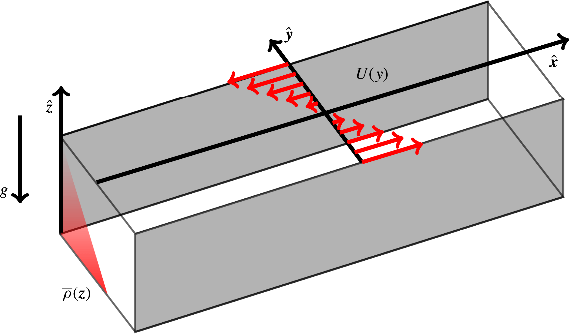
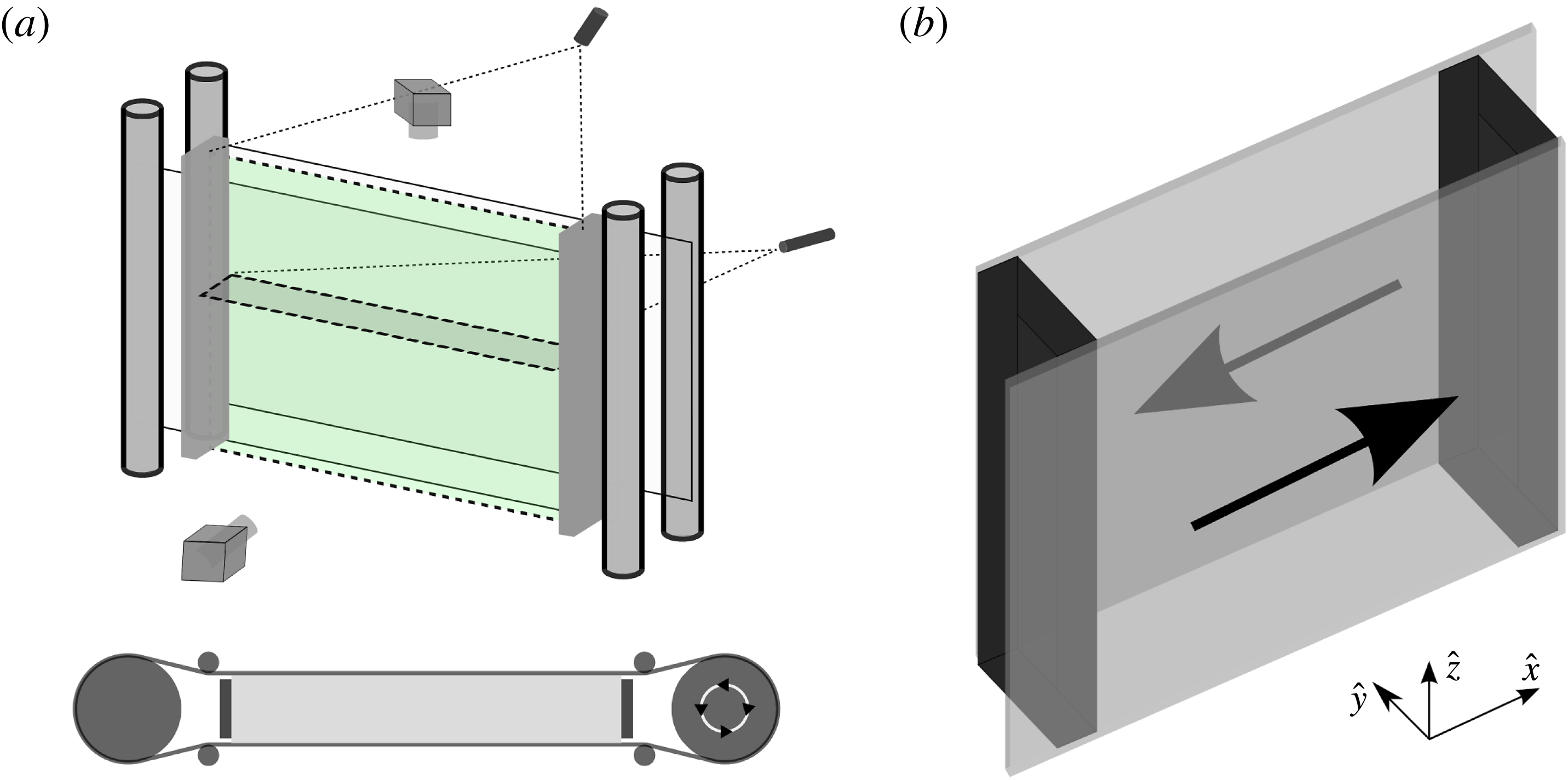
We consider the PC flow generated by two parallel walls moving with opposite velocities for a fluid which is stably stratified in density, as sketched in figure 1. We denote
 $\hat{\boldsymbol{x}}$
as the streamwise direction,
 $\hat{\boldsymbol{y}}$
as the cross-stream direction (i.e. the direction of the shear) and
 $\hat{\boldsymbol{z}}$
as the vertical direction (i.e. the direction of the stratification). The vector
 $\boldsymbol{g}$
denotes gravity while red arrows sketch the shape of the constant shear profile
 $U(y)$
and red shading mimics vertical stratification
 $\bar{\unicode[STIX]{x1D70C}}(z)$
. In the Boussinesq approximation we obtain the following system of equations:
 $$\begin{eqnarray}\displaystyle & \displaystyle \frac{\unicode[STIX]{x2202}\boldsymbol{u}}{\unicode[STIX]{x2202}t}+(\boldsymbol{u}\boldsymbol{\cdot }\unicode[STIX]{x1D735})\boldsymbol{u}=-\frac{\unicode[STIX]{x1D735}p^{\prime }}{\unicode[STIX]{x1D70C}_{0}}-\frac{\unicode[STIX]{x1D70C}^{\prime }}{\unicode[STIX]{x1D70C}_{0}}g\hat{\boldsymbol{z}}+\unicode[STIX]{x1D708}\unicode[STIX]{x1D6FB}^{2}\boldsymbol{u}, & \displaystyle\end{eqnarray}$$
 $$\begin{eqnarray}\displaystyle & \unicode[STIX]{x1D735}\boldsymbol{\cdot }\boldsymbol{u}=0, & \displaystyle\end{eqnarray}$$
 $$\begin{eqnarray}\displaystyle & \displaystyle \frac{\unicode[STIX]{x2202}\unicode[STIX]{x1D70C}^{\prime }}{\unicode[STIX]{x2202}t}+(\boldsymbol{u}\boldsymbol{\cdot }\unicode[STIX]{x1D735})\unicode[STIX]{x1D70C}^{\prime }-\frac{N^{2}}{g}\unicode[STIX]{x1D70C}_{0}w\hat{\boldsymbol{z}}=k\unicode[STIX]{x1D6FB}^{2}\unicode[STIX]{x1D70C}^{\prime }, & \displaystyle\end{eqnarray}$$
where we decompose the pressure and density fields
 $p$
and
 $\unicode[STIX]{x1D70C}$
into a perturbation
 $p^{\prime }$
and
 $\unicode[STIX]{x1D70C}^{\prime }$
and a stationary part
 $\bar{p}=p_{0}+\unicode[STIX]{x1D70C}_{0}gz-N^{2}z^{2}\unicode[STIX]{x1D70C}_{0}/2$
and
 $\bar{\unicode[STIX]{x1D70C}}=\unicode[STIX]{x1D70C}_{0}(1-N^{2}z/g)$
, with
 $p_{0}$
and
 $\unicode[STIX]{x1D70C}_{0}$
two constant reference values. We indicate with
 $N=\sqrt{-\unicode[STIX]{x2202}_{z}\bar{\unicode[STIX]{x1D70C}}(g/\unicode[STIX]{x1D70C}_{0})}$
the background Brunt–Väisälä frequency, while
 $\unicode[STIX]{x1D708}$
and
 $k$
denote constant viscosity and density diffusivity.
Sketch of the analysed flow in a Cartesian reference frame
 $\hat{\boldsymbol{x}}$
,
 $\hat{\boldsymbol{y}}$
,
 $\hat{\boldsymbol{z}}$
. The base flow is aligned with the streamwise direction
 $\hat{\boldsymbol{x}}$
, the constant shear is aligned with the cross-stream direction
 $\hat{\boldsymbol{y}}$
, while density stratification and gravity are aligned with the vertical direction
 $\hat{\boldsymbol{z}}$
. We highlight no-slip lateral boundaries in grey. Open periodic boundaries are not coloured.

2.1 Linear stability analysis
We perform the linear stability analysis of (2.1)–(2.3) in a Cartesian box of dimensions
 $(L_{x},L_{y},L_{z})$
centred at
 $x=y=z=0$
. With this aim we introduce the buoyancy
 $b=\unicode[STIX]{x1D70C}^{\prime }g/\unicode[STIX]{x1D70C}_{0}$
and decompose the velocity
 $\boldsymbol{u}$
into a base flow
 $\boldsymbol{U}=-\boldsymbol{U}_{0}y\hat{\boldsymbol{x}}$
and a perturbation
 $\boldsymbol{u}^{\prime }$
. Boundary conditions are periodic in the streamwise and vertical directions and no slip, i.e.
 $\boldsymbol{u}^{\prime }=\mathbf{0}$
, at the rigid walls
 $y=\pm L_{y}/2$
. Buoyancy perturbations
 $b$
are also set to 0 at the walls. The system is made non-dimensional using the length
 $L_{0}=L_{y}/2$
, the density
 $\unicode[STIX]{x1D70C}_{0}$
and the velocity
 $U_{0}=\unicode[STIX]{x1D70E}L_{0}$
, where
 $\unicode[STIX]{x1D70E}=-\unicode[STIX]{x2202}_{y}U(y)$
is the shear rate. This choice is consistent with Chen et al. (Reference Chen, Bai and Le Dizès2016) and gives the same set of dimensionless numbers, which are the Reynolds number
 $Re=L_{0}U_{0}/\unicode[STIX]{x1D708}$
, the Froude number
 $Fr=U_{0}/L_{0}N=\unicode[STIX]{x1D70E}/N$
and the Schmidt number
 $Sc=\unicode[STIX]{x1D708}/k$
. The dimensions of the box are fixed to
 $(L_{x}=131,L_{y}=2,L_{z}=14)$
. We then look for solutions of the non-dimensional perturbations
 $\tilde{\boldsymbol{u}},\tilde{p}$
and
 $\tilde{b}$
in the form of normal modes
 $$\begin{eqnarray}\tilde{\boldsymbol{u}},\tilde{p},\tilde{b}=(\boldsymbol{u}(y),p(y),b(y))\text{e}^{\text{i}k_{x}x+\text{i}k_{z}z-\text{i}\unicode[STIX]{x1D714}t},\end{eqnarray}$$
where we again use symbols
 $\boldsymbol{u}$
,
 $p$
and
 $b$
to simplify notations. Substituting in (2.1)–(2.3) and retaining only the first-order terms we obtain:
 $$\begin{eqnarray}\displaystyle & \displaystyle -\text{i}\unicode[STIX]{x1D714}u=\text{i}k_{x}uy+v-\text{i}k_{x}p+\frac{1}{Re}\unicode[STIX]{x1D6E5}_{y}u, & \displaystyle\end{eqnarray}$$
 $$\begin{eqnarray}\displaystyle & \displaystyle -\text{i}\unicode[STIX]{x1D714}v=\text{i}k_{x}vy-\frac{\text{d}p}{\text{d}y}+\frac{1}{Re}\unicode[STIX]{x1D6E5}_{y}v, & \displaystyle\end{eqnarray}$$
 $$\begin{eqnarray}\displaystyle & \displaystyle -\text{i}\unicode[STIX]{x1D714}w=\text{i}k_{x}wy-\frac{b}{Fr^{2}}-\text{i}k_{z}p+\frac{1}{Re}\unicode[STIX]{x1D6E5}_{y}w, & \displaystyle\end{eqnarray}$$
 $$\begin{eqnarray}\displaystyle & \displaystyle 0=\text{i}k_{x}u+\text{i}k_{z}w+\frac{\text{d}v}{\text{d}y}, & \displaystyle\end{eqnarray}$$
 $$\begin{eqnarray}\displaystyle & \displaystyle -\text{i}\unicode[STIX]{x1D714}b=\text{i}k_{x}by+w+\frac{1}{ReSc}\unicode[STIX]{x1D6E5}_{y}b, & \displaystyle\end{eqnarray}$$
where we denote with
 $\unicode[STIX]{x1D6E5}_{y}$
the Laplacian operator
 $\unicode[STIX]{x1D6E5}_{y}=\text{d}^{2}/\text{d}y^{2}-k_{x}^{2}-k_{z}^{2}$
. The system of equations above is solved using a pseudo-spectral approach similar to Chen et al. (Reference Chen, Bai and Le Dizès2016), the only difference being that discretization is made on the Gauss–Lobatto collocation points of the Chebyshev polynomials (i.e. instead of Laguerre polynomials) because this choice is well adapted to a two-side bounded domain. The generalized eigenvalue problem
 $\boldsymbol{A}\boldsymbol{f}=\unicode[STIX]{x1D714}\boldsymbol{B}\boldsymbol{f}$
for
 $\boldsymbol{f}=[u,v,w,b,p]$
is solved with the QZ algorithm. In parallel we also consider the inviscid approach, which consists in neglecting both viscous dissipation and salt diffusion, thus reducing the system (2.5)–(2.9) to one equation for the pressure:
 $$\begin{eqnarray}\frac{\unicode[STIX]{x2202}^{2}p}{\unicode[STIX]{x2202}y^{2}}-\frac{2k_{x}}{\unicode[STIX]{x1D714}_{\ast }}\frac{\unicode[STIX]{x2202}p}{\unicode[STIX]{x2202}y}+\left(k_{z}^{2}\frac{\unicode[STIX]{x1D714}_{\ast }^{2}}{1-Fr^{2}\unicode[STIX]{x1D714}_{\ast }^{2}}-k_{x}^{2}\right)p=0,\end{eqnarray}$$
where
 $\unicode[STIX]{x1D714}_{\ast }=\unicode[STIX]{x1D714}+k_{x}y$
. The equation above is analogous to that provided by Kushner, McIntyre & Shepherd (Reference Kushner, McIntyre and Shepherd1998), who previously studied the stability of a vertically stratified PC flow in the presence of rotation
 $f$
. In the limit of no rotation (
 $f\rightarrow 0$
) we verify that the two equations are the same, but contrary to Kushner et al. (Reference Kushner, McIntyre and Shepherd1998) we could not find a meaningful limit in which our equation (2.10) becomes autonomous in
 $y$
. As a consequence we cannot provide a compact form for the dispersion relation. Nevertheless, looking at (2.10) is still extremely instructive. First, one observes that the second term in (2.10) possibly diverges at
 $y=0$
when considering stationary modes which are marginally stable (e.g.
 $\unicode[STIX]{x1D714}=0$
). This corresponds to the existence of a barotropic critical layer, which happens to be regularized because, from the symmetry of the base flow, we expect
 $\unicode[STIX]{x2202}p/\unicode[STIX]{x2202}y$
to be null in
 $y=0$
for a stationary mode. Similarly the third term of (2.10) becomes critical in
 $y^{\ast }=\pm 1/k_{x}Fr$
when
 $\unicode[STIX]{x1D714}=0$
. These are baroclinic critical layers, i.e. the locations where the Doppler-shifted frequency
 $\unicode[STIX]{x1D714}_{\ast }$
of internal waves matches the Brunt–Väisälä frequency
 $N$
. In different contexts critical layers can be excited and have been observed in experiments (Boulanger, Meunier & Le Dizès Reference Boulanger, Meunier and Le Dizès2008) and numerical simulations (Marcus et al.
Reference Marcus, Pei, Jiang and Hassanzadeh2013). However, in our configuration, the most unstable mode is always observed to be stationary and at wavenumbers
 $k_{max}<1/Fr$
, which implies that the corresponding critical layers
 $y_{max}^{\ast }$
are always situated outside the numerical domain,
 $|y_{max}^{\ast }|>1$
.
3 Linear stability results
We have already mentioned that for unstratified fluids (i.e.
 $Fr=\infty$
) the PC (unperturbed) profile is linearly stable for any value of the Reynolds number
 $Re$
, thus we expect the flow to be potentially unstable only for finite values of the Froude number. The values of the Schmidt number for common salty water (i.e. in our experiments) is
 $Sc\sim 700$
, thus we first consider the limit
 $Sc=\infty$
and discuss the quality of this approximation at the end of this section.
As a first result we report that one stationary growing mode (i.e.
 $\text{Im}(\unicode[STIX]{x1D714})>0$
,
 $\text{Re}(\unicode[STIX]{x1D714})=0$
) appears at
 $Fr\lesssim 1$
, wavenumbers
 $k_{x}\sim 0.8$
,
 $k_{z}\sim 5$
and remarkably moderate Reynolds number
 $Re\simeq 700$
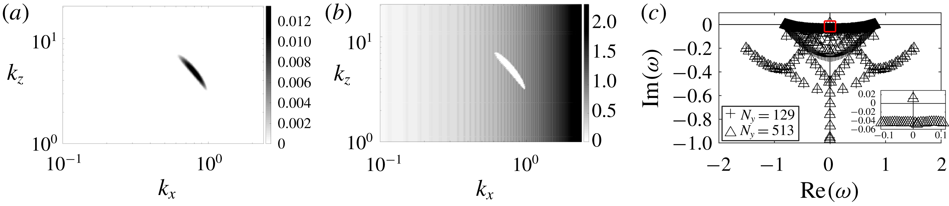
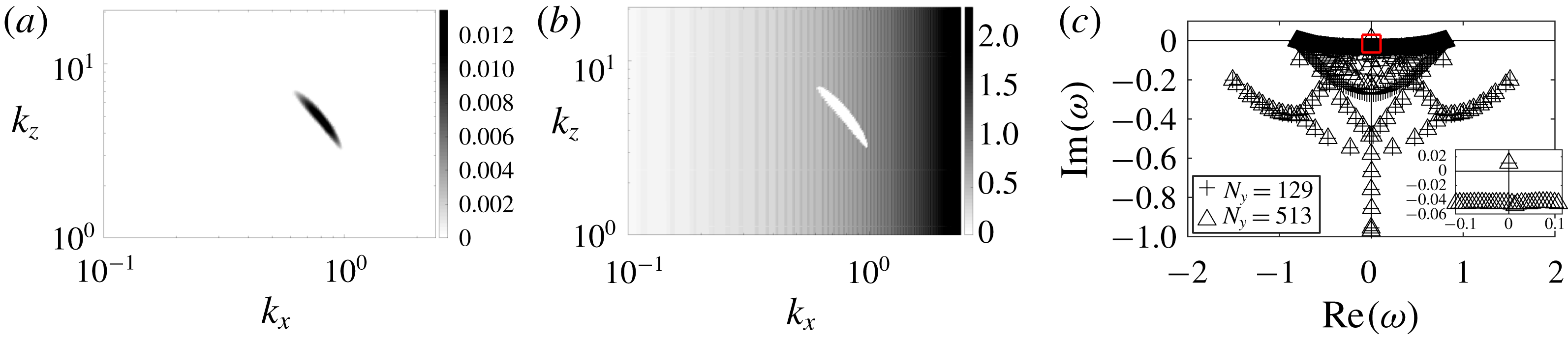
. In figure 2 we report the value of the imaginary part and the real part of the most unstable eigenmode for
 $Re=10^{3}$
and
 $Fr=1$
as a function of
 $k_{x}$
and
 $k_{z}$
. Looking at the imaginary part in figure 2(a) one sees that the flow is unstable over a narrow elongated region centred in
 $k_{x}\sim 0.8$
,
 $k_{z}\sim 5$
and stable elsewhere. Correspondingly the real part in figure 2(b) is zero whenever the flow is unstable and non-zero elsewhere. In figure 2(c) we also report the values of the temporal frequency
 $\unicode[STIX]{x1D714}$
for all the eigenvalues and two numbers of collocation points (
 $N_{y}=129$
and 513) for the most unstable wavenumbers (
 $k_{x}=0.815$
,
 $k_{z}=4.937$
). Eigenvalues which are well resolved correspond to the points where two different symbols are superposed, all other points are not well resolved, presumably because of the infinite value of
 $Sc$
considered here. The inset close to the origin of the diagram shows that a unique eigenvalue is present for which
 $\text{Im}(\unicode[STIX]{x1D714}_{c})>0$
. The value of
 $\unicode[STIX]{x1D714}_{c}$
is stable to the variation of
 $N_{y}$
, the number of collocation points, which indicates that the mode is well resolved. Finally, we remark that as our flow is bounded at
 $y=\pm 1$
, we do not have to deal with the problem of neutral or stable non-physical eigenvalues encountered by Chen et al. (Reference Chen, Bai and Le Dizès2016), which arises when prescribing the boundary condition at infinity.
When increasing
 $Re$
, the unstable region in the (
 $k_{x}$
,
 $k_{z}$
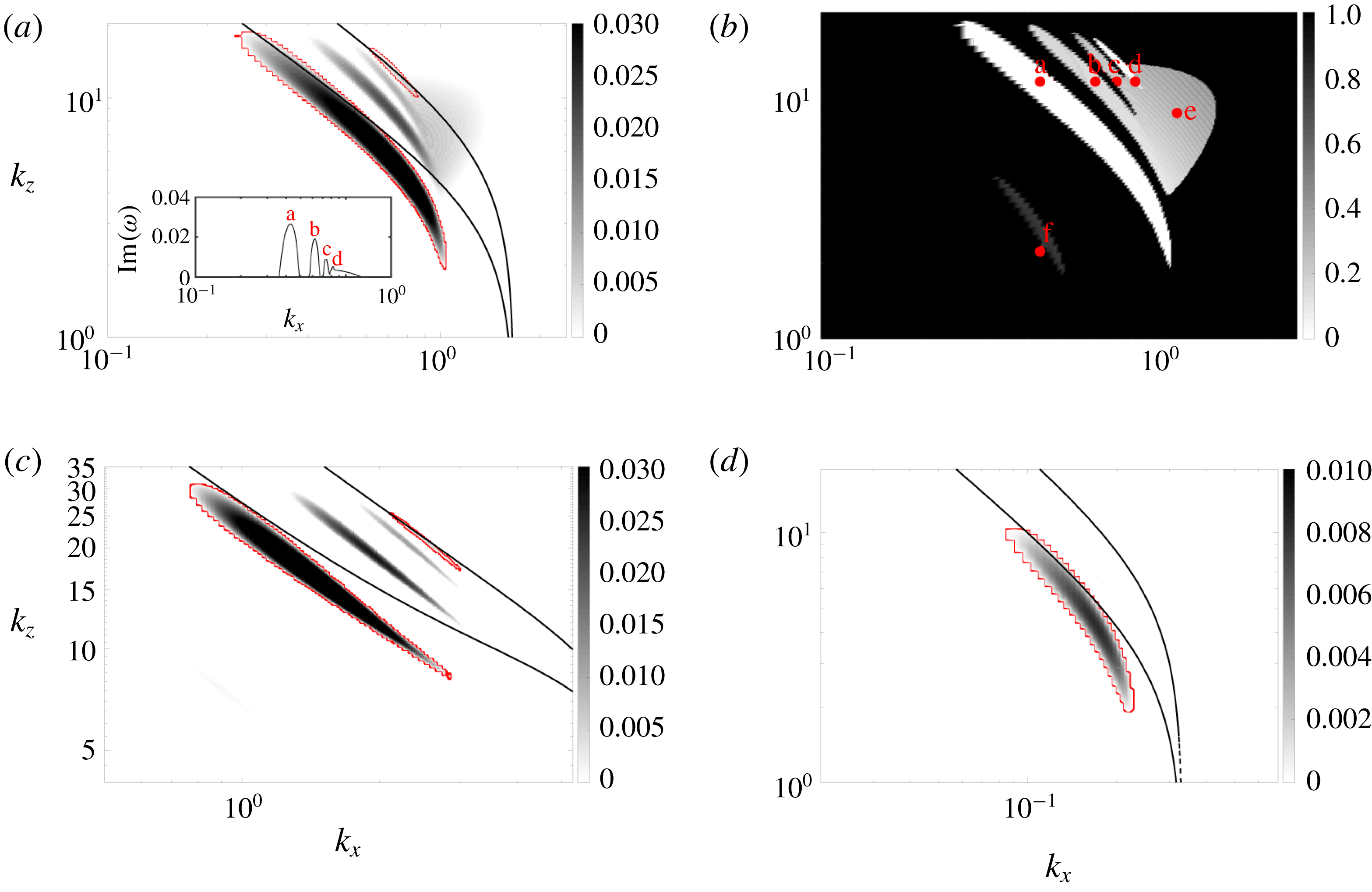
) space increases and unstable modes exist over a larger range of Froude number. In figure 3(a,b) we report the value of
 $\text{Im}(\unicode[STIX]{x1D714})$
and
 $C$
for the most unstable mode at
 $Re=10^{4}$
and
 $Fr=1$
, where we define
 $C$
as the quantity
 $C=\text{Re}(\unicode[STIX]{x1D714})/k_{x}$
. In the same figure we report similar graphs for
 $\text{Im}(\unicode[STIX]{x1D714})$
at
 $Re=10^{4}$
,
 $Fr=0.2$
(panel c) and
 $Fr=5$
(panel d). Note that at these values of
 $Fr$
number there is no unstable mode at
 $Re=10^{3}$
.
(a) Growth rate
 $\text{Im}(\unicode[STIX]{x1D714})$
of the most unstable mode in the space
 $(k_{x},k_{z})$
at
 $Fr=1$
and
 $Re=10^{3}$
. (b) Oscillation frequency
 $\text{Re}(\unicode[STIX]{x1D714})$
of the most unstable mode in the space
 $(k_{x},k_{z})$
at
 $Fr=1$
and
 $Re=10^{3}$
. Note that unstable modes (
 $\text{Im}(\unicode[STIX]{x1D714})>0$
) are stationary (
 $\text{Re}(\unicode[STIX]{x1D714})=0$
). (c) Full spectrum at the most unstable mode
 $k_{x}=0.815$
and
 $k_{z}=4.937$
,
 $Fr=1$
and
 $Re=10^{3}$
. Crosses refer to
 $N_{y}=129$
collocation points and triangles to
 $N_{y}=513$
collocation points. The inset at the bottom right coincides with the area delimited by the red rectangle.
(a,b) Growth rate
 $\text{Im}(\unicode[STIX]{x1D714})$
(a) and
 $C=\text{Re}(\unicode[STIX]{x1D714})/k_{x}$
(b) of the most unstable modes in the space
 $(k_{x},k_{z})$
at
 $Re=10^{4}$
and
 $Fr=1$
. Red dots and letters label modes of different shapes. The inset in (a) shows the value of
 $\text{Im}(\unicode[STIX]{x1D714})$
as a function of
 $k_{x}$
for a constant value of
 $k_{z}=10.77$
. (c,d) Growth rate
 $\text{Im}(\unicode[STIX]{x1D714})$
of the most unstable modes at
 $Re=10^{4}$
, with
 $Fr=0.2$
(c) and
 $Fr=5$
(d). The red contours distinguish stationary branches from oscillating branches. The black lines refer to the theoretical prediction we discuss in § 3.2, i.e. (3.2) for
 $n=1,2$
. Note that horizontal and vertical axes have different scales depending on the
 $Fr$
number.

One sees that at
 $Fr=1$
(panel a) the diagram is now richer: besides the original unstable branch constituted by stationary modes (a), new unstable branches appear at larger
 $k_{x}$
which correspond to oscillatory (b, c, e) and stationary (d) modes, as visible from the value of
 $\text{Re}(\unicode[STIX]{x1D714})/k_{x}$
(panel b). Note that within a particular branch the value of
 $\text{Re}(\unicode[STIX]{x1D714})/k_{x}$
varies very little, while the value of
 $\text{Im}(\unicode[STIX]{x1D714})$
shows a maximum, and smoothly decreases to zero at the branch boundaries. The quantity
 $\text{Re}(\unicode[STIX]{x1D714})/k_{x}$
then characterizes each different branch. A new oscillating branch (f) also appears at smaller
 $k_{x}$
but it is still very weak and poorly visible at this
 $Re$
number. In figure 3(c,d) we report the value of
 $\text{Im}(\unicode[STIX]{x1D714})$
in the space (
 $k_{x}$
,
 $k_{z}$
) at
 $Fr$
numbers smaller than and larger than one. When the Froude number is reduced to
 $Fr=0.2$
(panel c) we recover almost the same scenario, even if different branches now seem more spaced from one another and appear at larger
 $k_{x}$
and
 $k_{z}$
, similar to other kinds of shear flows (Deloncle et al.
Reference Deloncle, Chomaz and Billant2007; Park & Billant Reference Park and Billant2013). In contrast when the Froude number is increased to
 $Fr=5$
(panel d) the unstable region is drastically reduced, as well as the growth rate, which decreases by an order of magnitude. Also the most unstable mode moves towards lower values of
 $k_{x}$
while
 $k_{z}$
changes only slightly. As a general remark we observe that the unstable branches, i.e. the continuous regions defined by
 $\text{Im}(\unicode[STIX]{x1D714})>0$
, show an elongated shape. To be more precise, unstable regions appear extended when moving along the curve
 $k_{x}k_{z}=\text{const.}$
while they are quite narrow in the orthogonal direction. Also unstable modes always appear at
 $k_{z},k_{x}\neq 0$
, i.e. the flow is linearly unstable only to three-dimensional perturbations, which is different from the studies of Deloncle et al. (Reference Deloncle, Chomaz and Billant2007) and Lucas, Caulfield & Kerswell (Reference Lucas, Caulfield and Kerswell2017), performed on different vertically stratified and horizontally sheared flows (the hyperbolic tangent shear profile and Kolmogorov flow, respectively).
3.1 Stability diagram
We have explored the
 $(Re,Fr)$
parameter space over two decades around
 $Fr=1$
and for
 $Re$
from 500 to 50 000. For each combination
 $(Re,Fr)$
, we solve the system (2.5)–(2.9) in the discretized wavenumber space
 $k_{x}\in [0,2],k_{z}\in [0,30]$
, and look for all the possible linearly growing (
 $\text{Im}(\unicode[STIX]{x1D714})>0$
) modes. The (
 $k_{x}$
,
 $k_{z}$
) domain is suitably moved towards lower (respectively higher) wavenumbers when the
 $Fr$
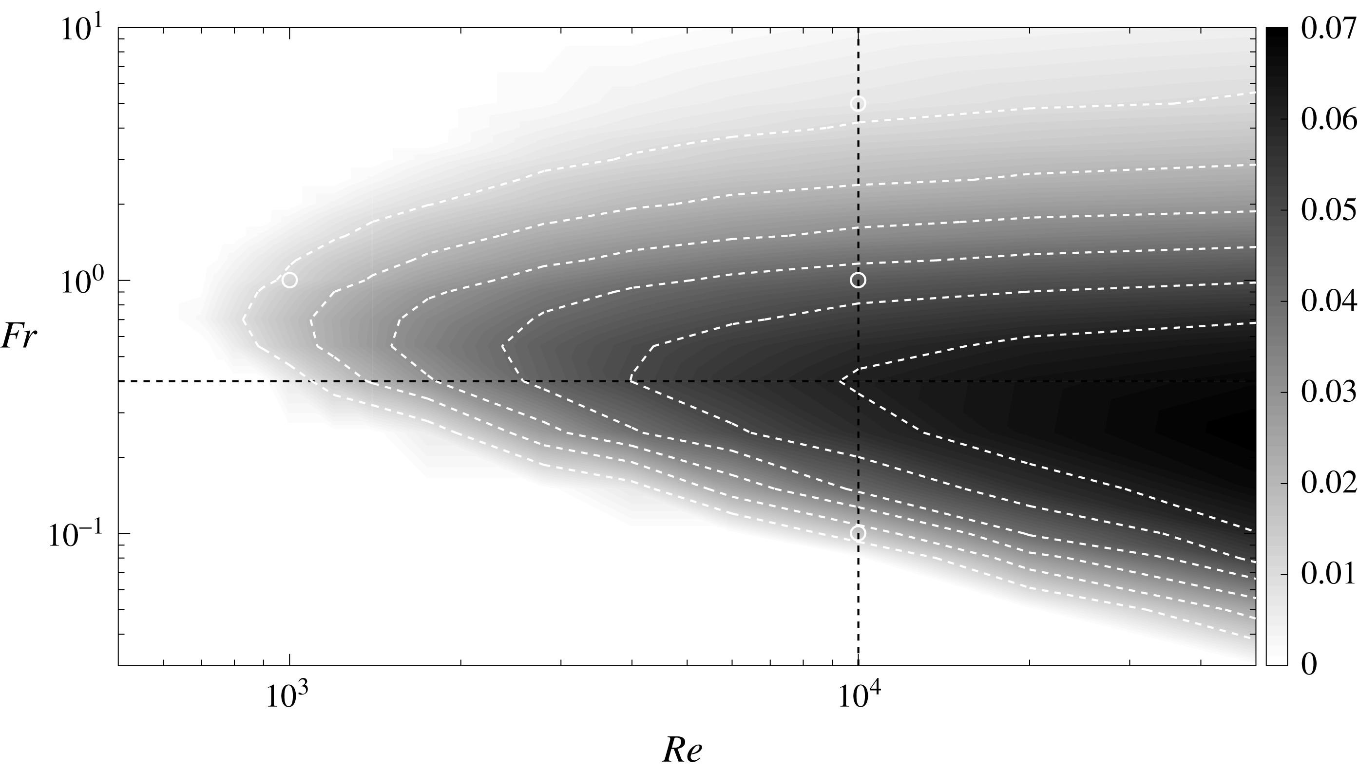
number is significantly higher (respectively lower) than 1. In figure 4 we report the stability diagram. Each point in the diagram corresponds to the most unstable mode, whose relative
 $k_{x}$
and
 $k_{z}$
generally vary. One observes that at
 $Re=10^{3}$
the unstable region is relatively constrained around
 $Fr=1$
(i.e.
 $0.5\lesssim Fr\lesssim 2$
), but already covers two decades in
 $Fr$
at
 $Re=10^{4}$
. This indicates that instability first (i.e. at low
 $Re$
number) appears where density stratification and horizontal shear are comparable, i.e.
 $N\sim \unicode[STIX]{x1D70E}$
, but is likely to be observed in a sensibly wider range of the ratio
 $\unicode[STIX]{x1D70E}/N$
provided that the
 $Re$
number is large enough.
Growth rate
 $\text{Im}(\unicode[STIX]{x1D714})$
of the most unstable mode in the space
 $(Re,Fr)$
. Each point is obtained by taking the maximum value of
 $\text{Im}(\unicode[STIX]{x1D714})$
over a collection of runs at fixed
 $(Re,Fr)$
and variable wavenumbers
 $(k_{x},k_{z})$
. White dashed contours correspond to
 $\text{Im}(\unicode[STIX]{x1D714})=0.01$
, 0.02, 0.03, 0.04, 0.05, 0.06. Black dashed lines correspond to
 $Re=10^{4}$
and
 $Fr=0.4$
. White circles correspond to the points of the diagram analysed in figures 2 and 3.

The critical Reynolds number (
 $Re_{c}\sim 700$
) appears quite moderate compared to other unstratified parallel flows such as plane Poiseuille flow (
 $Re_{c}=5772$
according to Orszag (Reference Orszag1971)). The value we find is comparable to the one found by Chen (Reference Chen2016) for a plane Poiseuille flow in the presence of vertical stratification, but still sensibly lower than the one indicated by the same authors (Chen et al.
Reference Chen, Bai and Le Dizès2016) for the boundary layer (vertically stratified) profile
 $Re_{c}\sim 1995$
. The growth rate is moderate even at high
 $Re$
number, indicating that the observed instability is not only constrained in
 $(k_{x},k_{z})$
but also relatively slow to establish.
Finally, we want to discuss how the most unstable mode changes as a function of the
 $Re$
and
 $Fr$
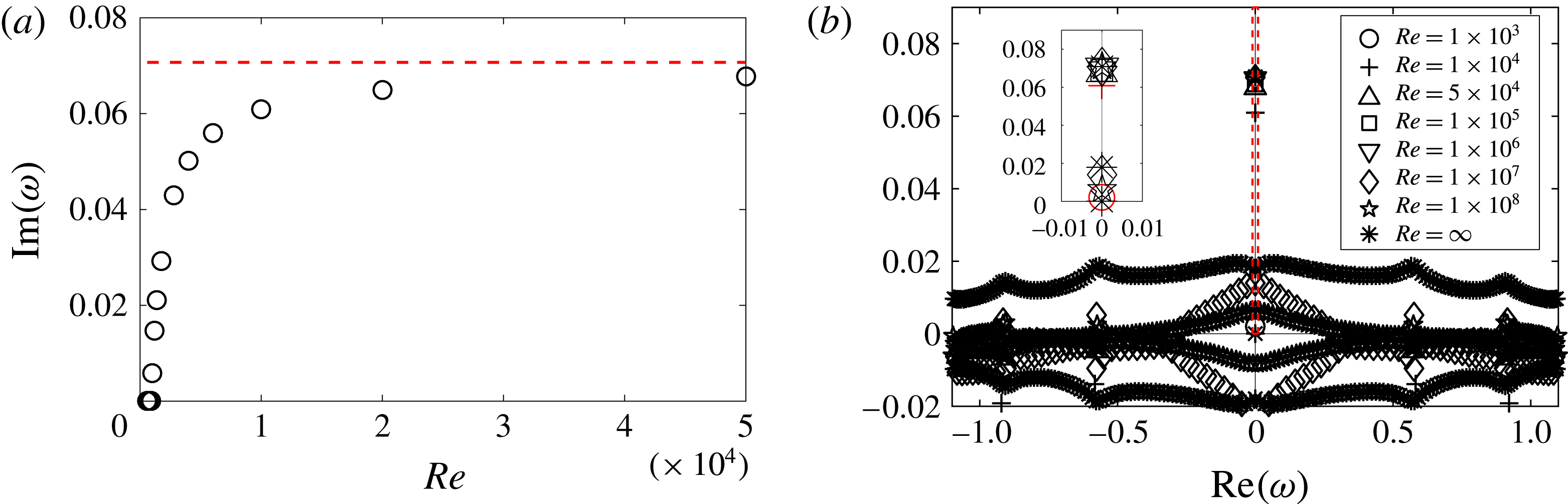
numbers separately. In figure 5 we analyse how the growth rate
 $\text{Im}(\unicode[STIX]{x1D714})$
of the most unstable mode (shown in panel a) changes with the
 $Re$
number at fixed
 $Fr=0.4$
. One sees that
 $\text{Im}(\unicode[STIX]{x1D714})$
rapidly saturates at a constant value. This result was confirmed by solving the eigenvalue problem (in panel b) at very high
 $Re$
number (up to
 $10^{8}$
) with
 $(k_{x},k_{z})$
fixed. In figure 6(a,b) we report the value of
 $k_{x}$
and
 $k_{z}$
for the most unstable mode as a function of
 $Re$
at fixed
 $Fr=0.4$
. One sees that both
 $k_{x}$
and
 $k_{z}$
tend to a constant value. Thus we conclude that the observed instability must rely on an inviscid mechanism and that the inviscid approximation is sufficient to capture the spatial
 $(k_{x},k_{z})$
and temporal (
 $\unicode[STIX]{x1D714}$
) features of the most unstable mode.
In figure 6(c,d) we report the value of
 $k_{x}$
and
 $k_{x}k_{z}$
for the most unstable mode as a function of the
 $Fr$
number at
 $Re=10^{4}$
. Panel (c) shows that
 $k_{x}$
is always slightly lower than
 $1/Fr$
(dashed line), which means that, for the most unstable mode, baroclinic critical layers (i.e.
 $y=\pm 1/k_{x}Fr$
) fall close to the boundaries but slightly outside the domain boundaries
 $y=\pm 1$
, and are likely not involved in the instability mechanism. In panel (d) we see that all solutions seem to collapse on the curve
 $A/Fr$
, where
 $A=k_{x}k_{z}|_{Fr=1}$
, which provides a rule for the spatial pattern of the most unstable mode and an interesting limit for further analysis of the pressure equation (2.10). Finally, one should note that, according to this relationship, in exploring the stability diagram
 $(Re,Fr)$
, the discretization of the wavenumber (i.e. the step size of the grid
 $kx,kz$
) becomes critical at low
 $Fr$
, while the size of the domain
 $(k_{x},k_{z})$
becomes critical at high
 $Fr$
.
(a)
 $\text{Im}(\unicode[STIX]{x1D714})$
(growth rate) of the most unstable mode as a function of the Reynolds number at
 $Fr=0.4$
. The dashed line corresponds to the inviscid solution as obtained by solving the eigenvalue problem. (b) Solutions of the eigenvalue problem at
 $Fr=0.4$
with fixed
 $k_{x}=1.29$
and
 $k_{z}=8.53$
. Different symbols correspond to different
 $Re$
numbers. The inset corresponds to the thin rectangular region indicated by the red dashed line in the main graph. We highlight in red the two lowest
 $Re$
numbers. One sees that starting from the third lowest one (
 $Re=5\times 10^{4}$
) the value of
 $\text{Im}(\unicode[STIX]{x1D714})$
saturates to an asymptotic value.

(a)
 $k_{x}$
as a function of
 $Re$
at
 $Fr=0.4$
, (b)
 $k_{z}$
as a function of
 $Re$
at
 $Fr=0.4$
, (c)
 $k_{x}$
as a function of
 $Fr$
at
 $Re=10^{4}$
and (d)
 $k_{x}k_{z}$
as a function of
 $Fr$
at
 $Re=10^{4}$
. In all the panels, circles correspond to the most unstable mode. The dashed line corresponds to a constant in (a,b) and to
 $1/Fr$
in (c,d).

3.2 The instability mechanism
So far we have focused only on the features of the most unstable mode for a given combination of the dimensionless numbers
 $Re$
,
 $Fr$
and a typical domain in the wavenumber space (
 $k_{x}$
,
 $k_{z}$
). This characterizes the instability from an operational point of view but gives no information about the underlying mechanism. To this end we now analyse the shape of unstable modes. We have seen that the asymptotic behaviour of the instability at large
 $Re$
number indicates that it relies on an inviscid mechanism. In the inviscid limit the pseudo-spectral approach is far less intelligible because the solution of the eigenvalue problem contains a large number of spurious modes with
 $\text{Im}(\unicode[STIX]{x1D714})>0$
, which makes detection of genuine unstable modes extremely difficult. The idea is then to consider a finite
 $Re$
number to keep the eigenvalue problem manageable but also large enough to capture all the possible features of the instability diagram. It turns out that the choice
 $Re=10^{4}$
responds reasonably well to these criteria; thus we focus on the case
 $Fr=1$
and
 $Re=10^{4}$
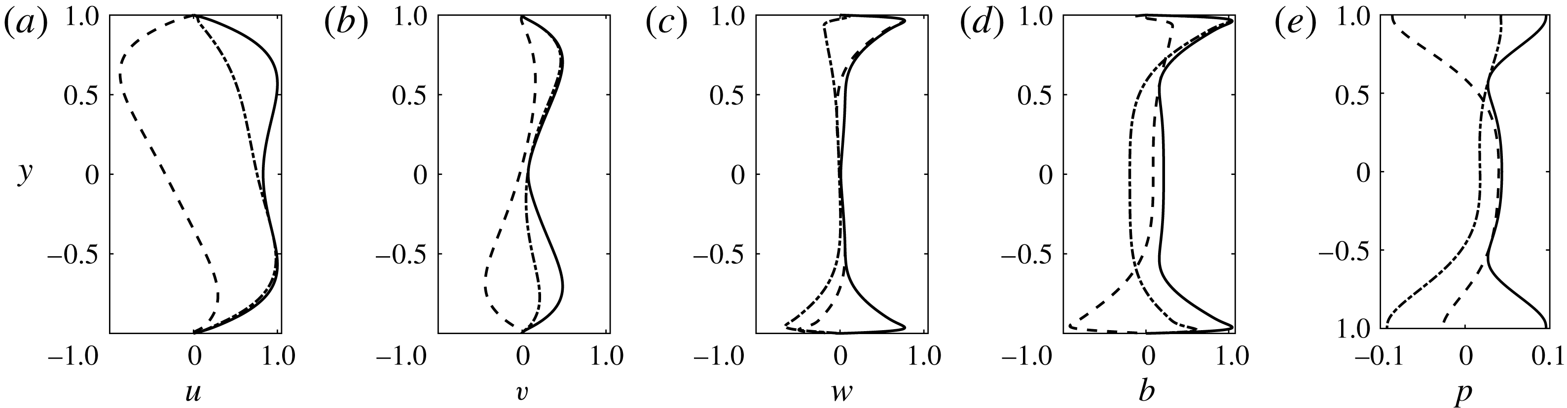
as a reference case. In figure 7 we report the eigenfunctions of the most unstable mode at
 $Fr=1$
and
 $Re=10^{4}$
, which corresponds to the wavenumbers
 $k_{x}=0.767$
and
 $k_{z}=4.937$
. One observes that the perturbations of the vertical velocity
 $w$
and buoyancy
 $b$
are more important close to the boundaries
 $y=\pm 1$
, while at the centre of the domain
 $y=0$
, the velocity perturbation is mainly horizontal.
Eigenfunctions of the most unstable mode at
 $Fr=1$
,
 $Re=10^{4}$
and wavenumbers
 $k_{x}=0.767$
,
 $k_{z}=4.937$
. Velocity fields and buoyancy are rescaled by dividing by the maximum value of the perturbation
 $u$
. Solid lines refer to the absolute value, while dashed and dashed-dotted lines refer to the real and imaginary parts, respectively.

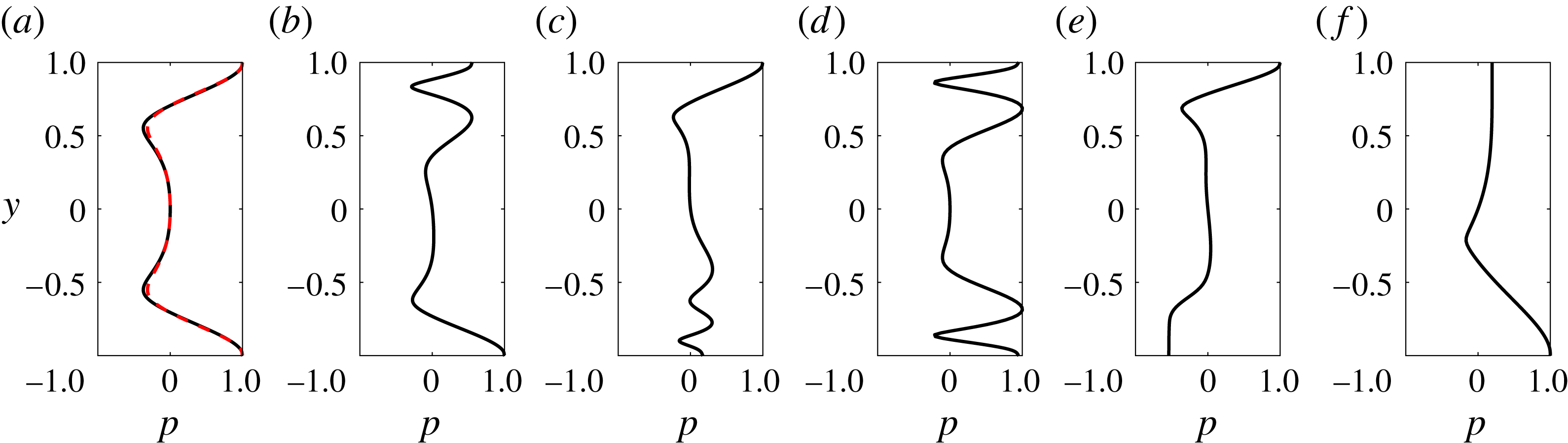
Modulus of the pressure eigenmodes for
 $Re=10^{4}$
,
 $Fr=1$
at
 $k_{z}=10.77$
with
 $k_{x}=0.432$
(a),
 $k_{x}=0.624$
(b),
 $k_{x}=0.719$
(c),
 $k_{x}=0.815$
(d). (e) Modulus of the pressure mode with
 $k_{x}=1.055$
and
 $k_{z}=8.078$
. (f) Modulus of the pressure mode with
 $k_{x}=0.432$
and
 $k_{z}=2.693$
. In (a) the red dashed line corresponds to the most unstable mode, i.e. the same as in figure 7(e). One observes that two modes belonging to the same branch are very close.

We now consider a sample mode for each different unstable branch – for example, corresponding to the red spots we labelled (a–f) in figure 3. In figure 8 we compare the pressure eigenmode for all different branches. One observes that the shape of the eigenmodes is significantly different in each panel. Not surprisingly, modes from the two stationary branches (panels a,d) are symmetric in the cross-stream direction
 $y$
. Conversely, travelling modes (panels b,c,e,f) are asymmetric but always appear in pairs, at
 $\unicode[STIX]{x1D714}_{\pm }=\pm \text{Re}(\unicode[STIX]{x1D714})+\text{i}\,\text{Im}(\unicode[STIX]{x1D714})$
, each mode in a pair being the
 $y$
-mirror of the other with respect to
 $y=0$
. Also in panel (a) we superpose the pressure eigenfunction of the most unstable mode at
 $k_{x}=0.767$
and
 $k_{z}=4.937$
, i.e. the same as figure 7(e). One should note that two pressure eigenmodes belonging to the same branch have basically the same shape.
The scenario we described above is strikingly similar to that presented by Satomura (Reference Satomura1981) (see, for example, his figure 6), who analysed the stability of a non-stratified PC flow in the shallow-water approximation. In this case the pressure
 $p$
is replaced by the elevation of the free surface
 $h$
in the analogous equation to (2.10). The author suggested that the instability is produced by the resonance of two Doppler-shifted shallow-water waves. In this picture the (streamwise) phase velocity
 $C=\text{Re}(\unicode[STIX]{x1D714})/k_{x}$
of a shallow-water wave which travels close to one boundary can be approximated to that of a shallow-water wave in a fluid at rest plus a Doppler shift, say
 $U_{d}$
, which has the sign of the velocity of the considered boundary. Two distinct counterpropagating waves situated at opposite boundaries can then have the same phase speed and become resonant. Moreover, the resonant wavenumbers constitute a discrete spectrum because rigid walls make the dispersion relation of (non-sheared) waves discrete. More recently, the same mechanism was also reported to be responsible for linear instabilities in stratified, rotating PC (Vanneste & Yavneh Reference Vanneste and Yavneh2007) and stratified Taylor–Couette (Park & Billant Reference Park and Billant2013) flows. We suggest and show below that this interpretation remains valid in our case if we replace shallow-water gravity waves with internal gravity waves. The dispersion relation of the latter is also discrete and given by:
 $$\begin{eqnarray}C_{\pm }^{(n)}=\pm \frac{1}{k_{x}Fr}\sqrt{1-\frac{k_{z}^{2}}{k_{x}^{2}+k_{z}^{2}+n^{2}\unicode[STIX]{x03C0}^{2}}},\end{eqnarray}$$
where we use a notation slightly different from Satomura (Reference Satomura1981) (our
 $C$
corresponds to
 $C_{r}$
). Subscript
 $+$
(
 $-$
) refers to waves propagating in the positive (respectively negative) direction of the
 $x$
axis, while superscript
 $n$
labels different channel modes. Note that here the velocity
 $C$
does not correspond to the phase velocity (by definition this is
 $\text{Re}(\unicode[STIX]{x1D714})\hat{\boldsymbol{k}}/|\boldsymbol{k}|$
) of the wave nor to its horizontal component, but it is still the relevant quantity to describe the resonance mechanism.
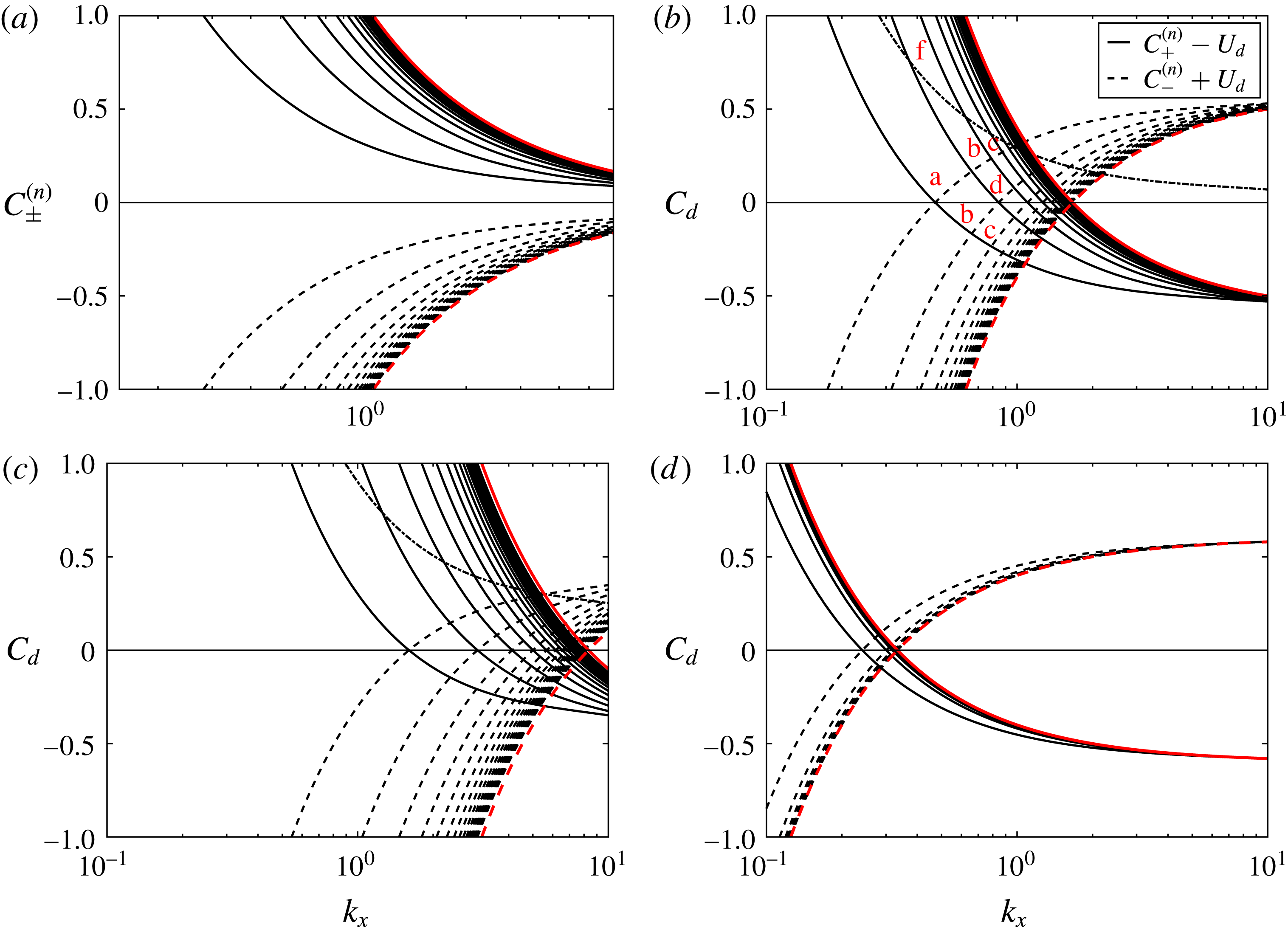
In figure 9(a) we report the value of
 $C_{\pm }^{(n)}$
as a function of
 $k_{x}$
at
 $k_{z}=10.77$
and
 $Fr=1$
. In panel (b) we show both Doppler-shifted velocities
 $C_{d}=C_{\pm }^{(n)}\mp U_{d}$
, where we consider prograde and retrograde waves moving upstream close to opposite boundaries and transported by the local mean flow. At this stage the value of
 $U_{d}$
is an adjustable parameter
 $-1\leqslant U_{d}\leqslant 1$
and was fixed to
 $U_{d}=0.6$
. This choice is somewhat arbitrary and can be avoided if one solves (2.10) and thus provides the exact dispersion relation in the presence of shear (Satomura Reference Satomura1981; Vanneste & Yavneh Reference Vanneste and Yavneh2007; Park & Billant Reference Park and Billant2013). In the present study we restrict ourselves to the phenomenological approach proposed by Satomura (Reference Satomura1981), and
 $U_{d}$
was taken as the flow velocity
 $U(y)$
at the
 $y$
coordinate where the pressure eigenfunctions of the first (a) and second (b) unstable modes appear to oscillate the most (see figure 8).
(a,b) Velocity
 $C_{\pm }^{(n)}$
as a function of
 $k_{x}$
as given by (3.1) at
 $k_{z}=10.77$
and
 $Fr=1$
and for the first
 $n=1$
–20 prograde (solid lines) and retrograde (dashed lines) confined internal gravity waves in the absence of mean flow (a), and the Doppler shifted velocities
 $C_{\pm }^{(n)}\mp U_{d}$
, where we set arbitrarily
 $U_{d}=0.6$
(b). The red lines indicate the limit of the dispersion relation for
 $n\rightarrow \infty$
, the crossing is situated at
 $k_{x}=1/FrU_{d}$
. We indicate with letters the resonances (crossing points) corresponding to different modes. Note that resonances (b) and (c) come in symmetric pairs. The single dashed-dotted line corresponds to
 $C_{+}^{(1)}$
, i.e. a non-transported prograde
 $n=1$
mode. (c,d) Same as (b) but at
 $Fr=0.2$
,
 $k_{z}=18$
(c) and
 $Fr=5$
,
 $k_{z}=3$
(d).

One can note that in the fixed frame (i.e.
 $U_{d}=0$
), prograde waves (solid lines) are well separated from retrograde waves (dashed lines). In contrast, for Doppler-shifted waves, there exists a discrete set of resonant
 $k_{x}$
where two curves of different type cross each other. At
 $Fr=1$
the first crossing (resonance) happens at
 $C_{d}=0$
and close to
 $k_{x}=0.4$
, which is consistent with the appearance of the first stationary mode (a) in the stability map of figure 3. The next two resonances happen at a non-zero value of
 $C_{d}$
which coherently recovers the appearance of the first two oscillating modes (b) and (c) at larger
 $k_{x}$
in figure 3. The following crossing happens again at
 $C_{d}=0$
, which confirms the appearance of a fourth (stationary) unstable branch in figure 3(b). Note that the appearance of the four modes a,b,c and d is clearly visible in the inset of figure 3(a), which reports
 $\text{Im}(\unicode[STIX]{x1D714})$
as a function of
 $k_{x}$
and at constant
 $k_{z}=10.77$
. Looking back at figure 8 the mode (f) appears to be the first half of mode (a), thus we speculate that the corresponding resonance originates from the crossing of a Doppler-shifted wave and a non-transported wave (i.e. one for which
 $U_{d}=0$
) situated at the centre of the domain (i.e. the dashed-dotted lines in figure 9). Mode (e) does not originate from a resonance, consequently it is not indicated in figure 9. A closer inspection of the velocity field suggests that in this case the baroclinic critical layers are excited, and the instability relies on a different mechanism. This hypothesis is consistent with the fact that the mode (e) (see figure 3) belongs to a region which mainly extends at
 $k_{x}>1/Fr$
where critical layers can fit within the domain.
Now that we have explained the origin of all the distinct modes as resulting from a degeneracy of the Doppler-shifted frequency, we want to show that this picture allows us to fully capture the shape of the unstable branches presented in figure 3. First, one should recall that for a given channel mode (i.e.
 $n=\text{const.}$
), the dispersion relation of internal gravity waves (3.1) is a function of two variables
 $k_{x}$
and
 $k_{z}$
, and hence is a surface. It follows that degeneracy occurs indeed on the intersection of two surfaces (i.e. not two curves), which is a curve (i.e. not a single point). The latter explains why the shape of the unstable branches presented in figure 3 appears elongated in one direction and constrained in the orthogonal direction. In the particular case of a stationary mode, one can easily deduce the equation of such a curve from the dispersion relation (3.1) modified by the Doppler shift
 $U_{d}$
. We find
 $$\begin{eqnarray}k_{z}={\mathcal{F}}(k_{x},n,Fr,U_{d})=\sqrt{\frac{n^{2}\unicode[STIX]{x03C0}^{2}}{U_{d}^{2}Fr^{2}k_{x}^{2}}-k_{x}^{2}-n^{2}\unicode[STIX]{x03C0}^{2}+\frac{1}{Fr^{2}U_{d}^{2}}}.\end{eqnarray}$$
In figure 3 we have superimposed the value of
 ${\mathcal{F}}$
on the map of the growth rate
 $\text{Im}(\unicode[STIX]{x1D714})$
at different
 $Fr$
numbers and for
 $n=1$
and 2. The agreement is not only qualitative – for example
 ${\mathcal{F}}$
reproduces the trend
 $k_{x}k_{z}\approx \text{const.}$
observed before – but also quantitative, because fixing a unique value of
 $U_{d}=0.6$
, we are able to predict the position of almost all the unstable stationary branches.
Finally, we show that the mechanism we describe above allows one to predict the boundaries of the unstable region. If we look back at figure 9 one observes that instability appears at a finite value of
 $k_{x}$
, say
 $k_{x}^{inf}$
, where
 $$\begin{eqnarray}C_{+}^{(1)}(k_{x}=k_{x}^{inf},n=1,k_{z},Fr)=U_{d}\end{eqnarray}$$
and must disappear when the envelopes of prograde and retrograde modes (red lines) cross each other, at
 $k_{x}^{sup}=1/FrU_{d}$
. Note that the latter upper boundary is independent of
 $k_{z}$
. Conversely the lower boundary can be arbitrarily reduced – for example, taking the limit
 $k_{x}^{inf}\rightarrow 0$
in (3.2) one has
 $k_{z}\rightarrow \infty$
. Nevertheless, any finite
 $Re$
number will likely inhibit an instability appearing at large wavenumber
 $k_{z}$
. We conclude that according to the proposed resonance mechanism, the instability is triggered by perturbations which are not streamwise invariant (i.e.
 $k_{x}\neq 0$
), and at streamwise wavenumber
 $k_{x}<1/FrU_{d}$
. Looking at the growth rate diagrams of figure 3 one actually sees that
 $k_{x}^{sup}$
tends to overestimate the upper bound of the unstable region. We suspect that a better prediction would be obtained by computing the exact dispersion relation in the presence of shear, as already done in analogous works (Satomura Reference Satomura1981; Vanneste & Yavneh Reference Vanneste and Yavneh2007; Park & Billant Reference Park and Billant2013) about Doppler-induced wave resonances. Figure 9(c,d) illustrates the same resonance mechanism for
 $Fr=0.2$
and
 $Fr=5$
. Panel (c) (
 $Fr=0.2$
) confirms that the instability range is extended and pushed at larger
 $k_{x}$
for small
 $Fr$
number (i.e. high stratification). Conversely, panel (d) (
 $Fr=5$
) shows that the region where resonances take place both shrinks and is constrained to smaller
 $k_{x}$
. Ultimately,
 $k_{x}^{inf}$
and
 $k_{x}^{sup}$
collide in the limit
 $Fr\rightarrow \infty$
and the instability likely disappears or at least reduces to an infinitely narrow range in
 $k_{x}$
. Note that the results above suggest that the upper boundary of the unstable region in figure 4 is intrinsic to the instability mechanism, while the lower boundary is controlled by the
 $Re$
number: at small
 $Fr$
, instability appears at larger
 $k_{x}$
, which corresponds to larger
 $k_{z}$
and is then more sensitive to viscous dissipation. To conclude this section we recall that if the growth rate varies with the
 $Re$
number, and different branches appear at different
 $Re$
numbers, the value of
 $C$
on a particular branch is approximately constant and is almost constant with the
 $Re$
number. This supports the hypothesis of a resonance and confirms that the appearance of the most unstable stationary and oscillating modes relies on an inviscid mechanism.
3.3 Effect of the Schmidt number
All the results presented above correspond to solutions of the eigenvalue problem where mass diffusivity was completely neglected, that is
 $Sc=\infty$
. We have modified the eigenvalue problem and tested the relevance of a finite
 $Sc$
number for the reference case
 $Re=966$
and
 $Fr=0.82$
, which will serve as a comparison between linear analysis, experiments and direct numerical simulations. All the computations are performed at the wavenumbers
 $k_{x}=0.96$
,
 $k_{z}=5.16$
, where the most unstable mode appears in the
 $Sc=\infty$
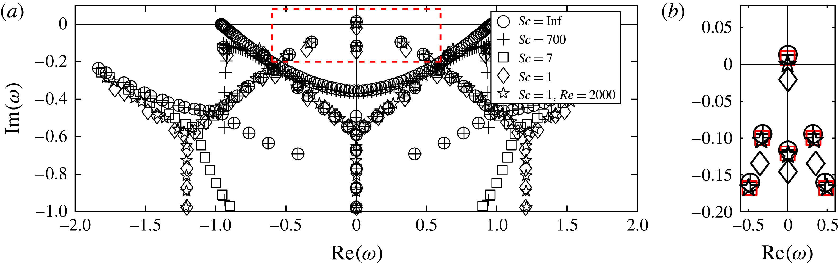
case. The results are reported in figure 10. First, we report that at
 $Sc=\infty$
(circles) and
 $Sc=700$
(crosses) the eigenvalues are well superimposed. This suggests that our non-diffusive approximation is qualitatively and quantitatively adequate to compare linear theory with experiments performed with salty water, for which
 $Sc=700$
. Second, we note that at
 $Sc=7$
(squares) there is still an unstable mode, and close to the origin the distribution of eigenvalues has the same form. For example, looking at the close up in figure 10(b), one sees that all the eigenvalues at
 $Sc=7$
(in red) are located close to a non-diffusive eigenvalue. This result makes possible the comparison between linear analysis, experiments and direct numerical simulations which will be performed at
 $Sc=7$
. Finally, we observe that at
 $Sc=1$
(diamonds and stars) the eigenvalues are distributed on three distinct Y-shaped branches, which is consistent with the previous study of Bakas & Farrell (Reference Bakas and Farrell2009) and Chen (Reference Chen2016), who found analogous branches at
 $Sc=1$
in the case of the PC flow and the plane Poiseuille flow, respectively. We also remark that at
 $Sc=1$
,
 $Re=966$
(diamonds) there is no unstable mode, nonetheless instability is promptly recovered at
 $Re=2000$
(stars). We conclude that the threshold value is not severely affected when increasing mass diffusion, as long as
 $Sc\gtrsim 7$
, although it may change when
 $Sc$
is of the order of unity.
(a) Eigenvalues in the complex space for the reference case
 $Re=966$
,
 $Fr=0.82$
,
 $k_{x}=0.96$
,
 $k_{z}=5.16$
and
 $Sc=\infty$
(circles),
 $Sc=700$
(crosses),
 $Sc=7$
(squares),
 $Sc=1$
(diamonds and stars). (b) Zoom on the region enclosed by the dashed red line in (a),
 $Sc=7$
symbols are reported in red.

4 Direct numerical simulations
In addition to the linear stability analysis, we have performed direct numerical simulations (DNS) of the full set of equations (2.1)–(2.3). The aim of a complementary DNS approach is to validate the linear theory and characterize the flow when retaining all the nonlinearities. Equations are solved in a rectangular box of dimensions (
 $L_{x},L_{y},L_{z}$
). The boundary conditions are periodic in both the streamwise and vertical directions, with rigid no-slip insulating boundaries in the cross-stream direction, i.e.
 $\boldsymbol{u}(y=\pm 1)=\mp \hat{\boldsymbol{x}}$
and
 $\text{d}b/\text{d}y=0$
at
 $y=\pm 1$
. In order to keep the computational time reasonable, while still focusing on the high-
 $Sc$
-number regime of the experiment described in § 5, we fix
 $Sc=7$
. We have seen in § 3.3 that this particular choice does not qualitatively affect the results, and in any case, ad hoc solutions of the linear problem at
 $Sc=7$
can be considered for a quantitative comparison. In order to ensure that the linear instability is well captured by the numerical simulation, we choose a box of size
 $(L_{x}=2\times \unicode[STIX]{x03C0}/k_{x},L_{y}=2,L_{z}=6\times \unicode[STIX]{x03C0}/k_{z})$
, where
 $k_{x}$
and
 $k_{z}$
are the most unstable wavenumbers as predicted by the linear stability analysis presented above.
We performed DNS using the spectral element solver Nek5000 (Fischer Reference Fischer1997; Fischer et al.
Reference Fischer, Loth, Lee, Lee, Smith and Bassiouny2007; see also http://nek5000.mcs.anl.gov). The use of spectral elements instead of more classical pseudo-spectral methods will be justified later (see § 5) where we add the effect of the streamwise confinement to mimic the experimental set-up. The global geometry is partitioned into hexahedral elements, with refinement close to the boundaries. Velocity, buoyancy and pressure variables are represented as tensor product Lagrange polynomials of order
 $N$
and
 $N-2$
based on Gauss or Gauss–Lobatto quadrature points. The total number of grid points is given by
 ${\mathcal{E}}N^{3}$
, where
 ${\mathcal{E}}$
is the number of elements. For all the results discussed in this paper, the number of elements is
 ${\mathcal{E}}=6336$
and we use a polynomial order from
 $N=7$
up to
 $N=11$
for the highest Reynolds number case. Time integration is performed with a backward difference explicit scheme for the advection and buoyancy terms, while viscous and dissipative terms are integrated using an implicit third-order scheme. The simulations are initialized with a small-amplitude buoyancy perturbation and with an established linear PC flow.
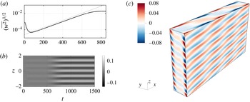
(a) Vertical kinetic energy
 $(\overline{w^{2}})^{1/2}$
as a function of time at
 $Re=966$
,
 $Fr=0.82$
and
 $Sc=7$
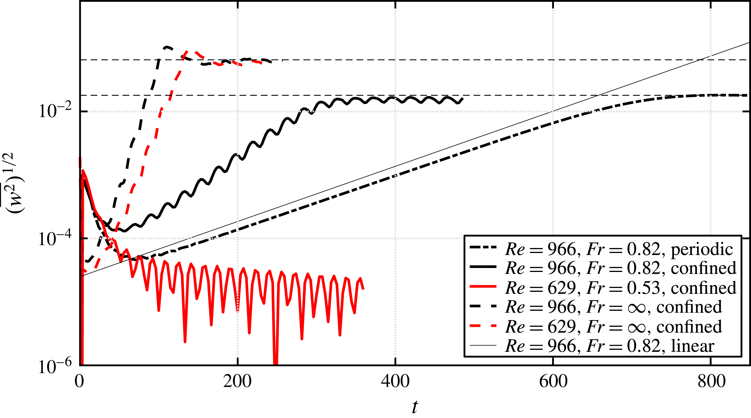
. The thick line refers to the DNS simulation while the thin line refers to the growth of the most unstable mode as indicated by linear stability analysis. (b) Horizontal velocity perturbation
 $u$
at
 $x=y=0$
as a function of
 $t$
and
 $z$
for the same DNS. One observes that a stationary pattern appears close to
 $t=500$
. (c) Instantaneous 3D map of the buoyancy perturbation once the flow has become unstable (DNS). As predicted by the linear analysis the selected mode is mainly modulated in the vertical direction but still not streamwise invariant (i.e.
 $k_{x}\neq 0$
). Note also that perturbations are concentrated near the boundaries
 $y=\pm 1$
.

In order to validate the eigenvalue problem we choose the reference case
 $Re=966$
,
 $Fr=0.82$
, which will serve later as a comparison to experiments. In figure 11(a) we report the time evolution of the rms vertical velocity (thick line), which is defined as:
 $$\begin{eqnarray}(\overline{w^{2}})^{1/2}=\left(\frac{1}{V}\int _{V}w^{2}\,\text{d}V\right)^{1/2},\end{eqnarray}$$
where
 $V$
refers to the volume of the simulation box. The quantity
 $(\overline{w^{2}})^{1/2}$
is appropriate since
 $(\overline{w^{2}})_{t=0}^{1/2}=0$
for the base flow. One observes that
 $(\overline{w^{2}})^{1/2}$
increases exponentially, and superposing the exponential growth predicted by the linear analysis one obtains an excellent agreement, with a relative discrepancy on the growth rate
 $\unicode[STIX]{x1D70E}_{c}$
of less than 1 %. In panel (b) we report the spatio-temporal diagram of the horizontal perturbation
 $u$
at
 $x=y=0$
. One observes that a stationary pattern has established around
 $t=500$
, which has a well-defined vertical wavelength. In figure 11(c) we report a visualization of the buoyancy perturbation
 $b$
once the instability has saturated. One observes a weakly inclined layering of the density field, which is a common feature in stratified, shear flows (see Thorpe Reference Thorpe2016, for a review). Again we have a very good agreement with the linear theory: a distinct spatial pattern appears and both vertical and horizontal wavelengths correspond to the predicted values. One can notice that the spatial pattern perfectly fits in the simulation domain. This condition is indeed necessary to observe the instability, and no relevant growth of the vertical kinetic energy is observed when none of the unstable wavenumbers fits inside the simulation domain.
5 Experiments
5.1 Experimental apparatus
Now, we want to study whether or not this linear instability of the stratified PC flow does appear in a ‘real’ configuration, and to do so, we look for some of its signatures in an experimental set-up, intrinsically limited in size. The flow is produced with a shearing device which is placed on the diagonal of a transparent tank (
 $50~\text{cm}\times 50~\text{cm}\times 70~\text{cm}$
) made of acrylic. The tank is filled with salty water linearly stratified in density. The shearing device is sketched in figure 12(a). The device consists of a PVC transparent belt (0.8 mm thick) which is closed on a loop around two vertical entraining cylinders made of dense sponge (we use standard spares entraining cylinders for commercial swimming-pool robots). Two additional pairs of cylinders (inox, 2 cm diameter) constrain the two sides of the loop to be parallel and at a controlled distance
 $d$
. All cylinders are mounted on a system of acrylic plates which allows the distance to be varied between the entraining cylinders (i.e. to tighten the belt) through two pairs of coupled screws (i.e. one pair for the bottom and one for the top). The top acrylic plates also prevent the existence of a free surface which would affect any imaging from the top. The motion of the belt is provided by a motor which is mounted on the top of the device and joined to the axis of one of the entraining cylinders. Finally, two PVC rigid plates are mounted vertically in front of the two entraining cylinders in order to reduce at most any perturbations coming from the entrainment system. The distance between the edges of the plates and the belt is a few millimetres. Thus we look at the flow in the area shaded in light grey (figure 12
a). In the present work we consider two values of the gap width
 $d=2L_{0}=5.8$
and 9.8 cm, while the distance between the PVC plates
 $D$
was respectively 34 cm and 24 cm, leading to a values of the aspect ratio (
 $D/d$
) of 5.7 and 2.4, respectively.
The tank is filled with salty water of variable density. As a general rule, a water column of height
 $H=10$
–20 cm linearly stratified in density always occupies the volume delimited by the belt and the confining barriers, while above and below the density stratification was generally weaker or negligible. The density profile is obtained by the double-bucket method (Oster Reference Oster1965). To measure the density profile we collect small samples of fluid (
 ${\sim}10~\text{ml}$
) at different heights and analyse them with a density-meter Anton Paar DMA 35. The Brunt–Väisälä frequency
 $N$
is constant for each experiment with a value between
 $0.5~\text{rad}~\text{s}^{-1}$
and
 $3.0~\text{rad}~\text{s}^{-1}$
. We measure the stratification before and after each experiment. The shearing motion clearly affects the stratification, especially through the small-scale features of the rotating part of the device, which necessarily produce some mixing. Also, in our highest-
 $Re$
experiments we observe optical distortion which indicates the presence of high-density gradients and thus layering similar to that observed in turbulent stratified experiments performed in Taylor–Couette devices (Oglethorpe, Caulfield & Woods Reference Oglethorpe, Caulfield and Woods2013). Nevertheless we observe that the density profile at the end of an experiment is weakly perturbed and the relative discrepancy with respect to the initial profile in the area of interest is approximately 5 %. Finally we assume the viscosity to be
 $\unicode[STIX]{x1D708}=10^{-6}~\text{m}^{2}~\text{s}^{-1}$
, and neglect any change associated with variable salt concentration.
(a) Sketch of the experimental shearing device seen from the side and from above. The two green shaded area correspond to two laser sheets which illuminate the mid vertical plane (i.e.
 $y=0$
) and the horizontal midplane (i.e.
 $z=0$
). Two cameras allow imaging of the flow in the illuminated areas. (b) Schematic of confined DNS experiments. Two rigid lateral walls entrain the fluid at constant velocity and two rigid walls confine the flow in the streamwise direction. Vertical boundary conditions are periodic.

The fluid is seeded with (
 $10~\unicode[STIX]{x03BC}\text{m}$
– diameter) hollow glass spheres and two laser sheets illuminate the particles in the vertical plane
 $y=0$
and the horizontal plane
 $z=0$
, as shown in figure 12. The flow is then recorded from the side by a 4 Mpx camera at a frame rate of 8 fps and from the top by a 2 Mpx camera at a frame rate of 30 fps. The velocity field is obtained with a particle image velocimetry (hereafter PIV) cross-correlation algorithm (Meunier & Leweke Reference Meunier and Leweke2003). Note that the mid vertical plane
 $y=0$
is the appropriate place to detect the possible onset of an instability because, in the ideal PC regime, the velocity should be zero there. The current set-up permits only single illumination and recording of the flow, thus movies from the top and from the side are always taken at different times.
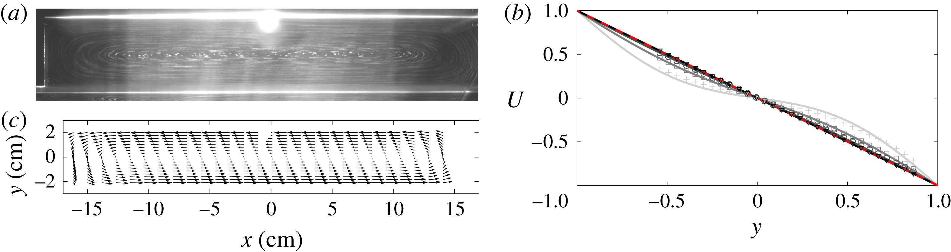
(a,c) Top view of the
 $z=0$
plane. We show a superposition of
 $40$
images (i.e.
 ${\sim}1.3~\text{s}$
) as captured by the camera (with only light contrast enhanced to show PIV particle trajectories) (a) and the velocity field
 $(u,v)$
as reconstructed via the PIV algorithm (c). The velocity plot is obtained by averaging over the 40 PIV fields (i.e.
 ${\sim}1.3~\text{s}$
). (b) Velocity cross-section at
 $x=0$
. Symbols refer to experimental observations, here
 $Re=533$
and
 $Fr=0.82$
. Each profile corresponds to the time average of the horizontal velocity fields over
 $0.03T_{\unicode[STIX]{x1D708}}$
. Solid lines refer to the value of the expression (5.1) expected for the two-infinite-walls problem (increasing time from clear grey to black). The dashed line refers to the asymptotic
 $t=\infty$
solution.

5.2 Base flow
First we report that a PC flow can be observed in the region confined between the belt and the PVC barriers. In figure 13(a) we superpose 40 images of the
 $z=0$
plane exactly as captured by the camera. Only the contrast was altered to enhance streamlines. Both the intersections of the belt with the laser sheet and the left barrier edge can be easily recognized as brighter lines. One also sees that streamlines close up near the PVC barriers and recirculations are present. This is confirmed by the velocity field given by the PIV algorithm shown in panel (c). The velocity plot is obtained by averaging over 40 PIV fields (
 ${\sim}1.3~\text{s}$
), also we plot only one arrow out of four in the horizontal direction, to make the diagram readable. One can note that up to 10 cm from the centre the flow is nicely parallel and the velocity gradient is linear. Both streamlines and PIV fields refer to an experiment where the base flow was already stationary. Now, any experiment necessarily implies a transient phase where the flow evolves from a first stationary phase, e.g. the whole fluid is at rest, to a second stationary phase which is the forced parallel flow. We expect the base flow to become established via viscous entrainment starting from the fluid layers which are close to the walls, thus the viscous time
 $T_{\unicode[STIX]{x1D708}}=d^{2}/\unicode[STIX]{x1D708}$
seems to be an appropriate time scale for the transient. In order to verify this we need some more quantitative prediction and consider the transient flow generated by two infinite walls treated by Acheson (Reference Acheson1990). As a first step, recirculations are neglected. If the flow is initiated at
 $t=0$
the horizontal velocity has the form
 $U(y,t)=U_{0}(y)-U_{T}(y,t)$
, where
 $U_{0}(y)$
is the asymptotic base flow and the transient part
 $U_{T}(y,t)$
reads:
 $$\begin{eqnarray}U_{T}(y,t)=(U_{0}-U_{i})\mathop{\sum }_{j=1}^{\infty }\frac{2}{\unicode[STIX]{x03C0}}\frac{(-1)^{j}}{j}\text{e}^{-\unicode[STIX]{x03C0}^{2}j^{2}t/Re}\sin j\unicode[STIX]{x03C0}y,\end{eqnarray}$$
where
 $U_{i}$
is the velocity of the belt at
 $t=0$
; for example,
 $U_{i}=0$
if the experiment is started with the fluid at rest. In figure 13 we compare the value of
 $U(y,t)$
as expected from (5.1) with the average value of the horizontal velocity as observed in a typical experiment. The value of
 $U$
is plotted as a function of
 $y$
at four different times. First, the velocity profile collapses on the expected PC flow (dashed line) around
 $t=T_{\unicode[STIX]{x1D708}}$
, which confirms that the base flow is established via viscous entrainment. Also at
 $t=T_{\unicode[STIX]{x1D708}}/3$
(circles), the value of the average horizontal velocity is already very close to the PC flow. Second, one can note an excellent agreement of the experimental observations with the infinite-walls approximation, which suggests that the recirculation does not significantly affect the shape of the transient flow. With regard to this, one should notice that knowing the time the base flow needs to become established is crucial when determining the growth rate of the instability, which will be discussed later.
Once the PC profile is established we want to detect possible deviations from the base flow. With this aim we mainly focus on the midplane
 $y=0$
, where no motion is expected for the base flow. As a standard protocol we initiate the flow at low shear rate
 $\unicode[STIX]{x1D70E}$
and then increase
 $\unicode[STIX]{x1D70E}$
by a small fraction (typically 15 %). Top views of the plane
 $z=0$
are also taken to verify the shape of the parallel base flow. In each experiment the flow was observed for at least one viscous time
 $T_{\unicode[STIX]{x1D708}}=d^{2}/\unicode[STIX]{x1D708}$
, which may be taken as an upper bound for establishing the base flow. First we report that starting from very moderate Reynolds number
 $Re\gtrsim 300$
the observed fluid oscillates coherently at a well-defined frequency. These bulk oscillations show a trivial pattern (i.e.
 $k_{x}=k_{y}=k_{z}=0$
) and are due to the periodic impact of the belt junction (which has some roughness) on the entraining cylinder. In the following we discuss how perturbations become more finely structured at higher
 $Re$
number, and we give a criterion to distinguish these initial deviations from a truly unstable pattern.
5.3 Instability
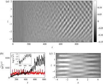
(a) Horizontal velocity perturbation
 $u$
at
 $x=y=0$
as a function of time. The colour bar is set to
 $\pm 15\,\%$
of the wall speed. Here
 $\unicode[STIX]{x1D70E}=1.15~\text{s}^{-1}$
,
 $Fr=0.82$
,
 $Re=969$
. All quantities are dimensionless. At
 $t=73.5$
the imposed shear switched from
 $0.34~\text{s}^{-1}$
to
 $1.15~\text{s}^{-1}$
. (b) Evolution of the mean horizontal perturbation
 $(\overline{u^{2}})^{1/2}$
as a function of time for the same experiment (black line) and for a stable experiment where both
 $Fr$
and
 $Re$
are reduced by 15 % (red line). The inset shows
 $\log (\overline{u^{2}})^{1/2}$
for the unstable case. At each time,
 $\overline{u^{2}}$
is obtained by averaging over a short interval
 ${\sim}4\unicode[STIX]{x1D70E}^{-1}$
, taking the square and finally averaging over the vertical direction. (c) Snapshot of the horizontal velocity perturbation
 $u$
in the plane
 $y=0$
; here
 $t\sim 900$
.

When the
 $Re$
number is sufficiently high
 $Re\gtrsim 1000$
and for Froude number
 $Fr\sim 1$
, an exponentially growing motion is observed to form in the midplane
 $y=0$
. The horizontal velocity perturbation
 $u$
shows a well-defined spatial pattern where horizontal and vertical wavelengths
 $\unicode[STIX]{x1D706}_{x}$
,
 $\unicode[STIX]{x1D706}_{z}$
can be detected reasonably well, with
 $\unicode[STIX]{x1D706}_{x}/\unicode[STIX]{x1D706}_{z}\sim 8$
. Results for this reference case are summarized in figure 14. On figure 14(a) we plot the horizontal velocity perturbation
 $u$
at
 $x=y=0$
as a function of the time
 $t$
and vertical direction
 $z$
. At
 $t\sim 73.5\unicode[STIX]{x1D70E}^{-1}$
the imposed shear has changed from a lower value of
 $\unicode[STIX]{x1D70E}=0.34~\text{s}^{-1}$
to
 $1.15~\text{s}^{-1}$
, and at
 $t\sim 550\unicode[STIX]{x1D70E}^{-1}$
one observes the appearance of a vertical wavelength. One also observes that the
 $t$
-periodic and
 $z$
-invariant bulk motion described in the previous section is present since the very beginning, and is still visible at large time, superposed on the instability pattern. In figure 14(b), we consider the time evolution of the order parameter
 $(\overline{u^{2}})^{1/2}$
for the same unstable case as above (black line) and for another case (red line) where the imposed shear,
 $\unicode[STIX]{x1D70E}$
is 15 % smaller. The average square of the horizontal perturbation
 $\overline{u^{2}}$
is computed at the centre vertical line
 $x=0,y=0$
in three steps starting from the spatio-temporal diagram of
 $u$
in panel (a). At each time we take the average of
 $u$
over a short interval
 ${\sim}4\unicode[STIX]{x1D70E}^{-1}$
, subtract the linear regression in
 $z$
, compute the square, and finally average over the vertical direction. We stress that subtracting the linear regression allows us to get rid of the bulk oscillations and of any possible top–bottom anisotropy due to a non-perfect verticality of the laser sheet. First, one can note that the unstable case (black line) shows a clear growth event of the order parameter which does not happen for the stable case (red line), thus indicating the appearance of an instability. Focusing on the unstable case one clearly sees that a first increase of
 $(\overline{u^{2}})^{1/2}$
occurs during the interval of
 ${\sim}0.3T_{\unicode[STIX]{x1D708}}$
after the change in the imposed shear, where the value of the viscous time is
 $T_{\unicode[STIX]{x1D708}}\sim 10^{3}\unicode[STIX]{x1D70E}^{-1}$
. At larger time,
 $\overline{u^{2}}$
increases again, now in an exponential way (see the inset on a semilog scale), and finally saturates at a constant value. The exponential growth rate is approximately
 $\unicode[STIX]{x1D714}\sim 0.06\unicode[STIX]{x1D70E}$
(although the noise makes a precise measurement of the growth rate difficult). We claim that the first growth phase coincides with the smooth progressive installation of the base PC flow at the imposed shear while the second growth phase corresponds to the onset of a linear instability. Note that for the stable case (red line) the first phase is less visible, because the shear
 $\unicode[STIX]{x1D70E}$
is imposed starting from a slightly lower value. Finally, on figure 14(c) we present a snapshot of the
 $u$
field in the plane
 $y=0$
. One observes a regular periodic pattern characterized by a vertical wavelength
 $\unicode[STIX]{x1D706}_{z}\sim 0.7L_{0}$
and a horizontal wavelength
 $\unicode[STIX]{x1D706}_{z}\sim 5.5L_{0}$
, where we recall that
 $L_{0}$
is half the width of the channel.
Below we consider the stability of our experimental flow in the
 $(Re,Fr)$
space, which is the same for the linear stability analysis performed in § 3.1. To this aim we need to define a common protocol to assess the presence or not of the instability. One criterion may be the appearance of a vertical wavelength. Unfortunately the latter is a smooth process; for example, a vertical wavelength was often visible at a shear
 $\unicode[STIX]{x1D70E}$
lower than what we assess to be the unstable case. Nevertheless, the associated signal was generally weak and no growth process was observed. The existence of the latter seems to be the most reliable criterion, but demands longer experiments and generally requires starting from very small
 $\unicode[STIX]{x1D70E}$
, which then requires slowing down the flow after each experiment. As a general rule we rather look at the saturated amplitude of the order parameter
 $(\overline{u^{2}})^{1/2}$
as a function of
 $\unicode[STIX]{x1D70E}$
and detect if an abrupt change occurs, as is clearly visible in figure 14 at large time. In particular
 $(\overline{u^{2}})^{1/2}$
is computed once the instability has saturated or alternatively after a time of the order of the viscous time
 $T_{\unicode[STIX]{x1D708}}$
after the actual value of the shear is imposed, to get rid of the base flow transient. We choose the control parameter
 $\unicode[STIX]{x1D70E}$
(i.e. the imposed shear) as the most suitable one, because it can be varied continuously, simply by controlling the speed of the entraining motor. As a drawback, both
 $Re$
and
 $Fr$
are linear in
 $\unicode[STIX]{x1D70E}$
, thus the stability diagram must be explored moving on tilted straight lines for which the ratio
 $Fr/Re=\unicode[STIX]{x1D708}/Nd^{2}$
is constant. Any change in the vertical stratification
 $N$
and gap width
 $d$
is considerably more laborious, which constrains the exploration of the
 $(Re,Fr)$
space to a few different
 $Fr/Re=\text{const.}$
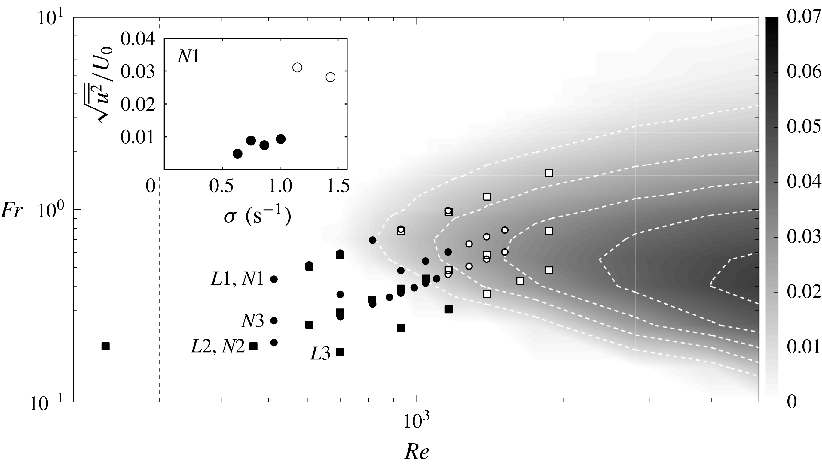
lines. In figure 15 we report six series of experiments performed at different values of
 $Fr/Re$
corresponding to different values of
 $N$
and
 $d$
. Experimental results are superposed on the linear stability diagram (figure 4). Experiments labelled
 $L1$
–
 $L3$
refer to large-gap experiments (
 $D/d=2.4$
) while those labelled
 $N1$
–
 $N3$
refer to narrow-gap experiments (
 $D/d=5.7$
). The value of
 $N$
ranges between 0.5 and
 $3.0~\text{rad}~\text{s}^{-1}$
. In the inset of the same figure we report the evolution of the quantity
 $(\overline{u^{2}})^{1/2}$
as a function of
 $\unicode[STIX]{x1D70E}$
for the experiment
 $N1$
. One sees that the order parameter abruptly increases when the imposed shear
 $\unicode[STIX]{x1D70E}$
crosses a threshold value
 $\unicode[STIX]{x1D70E}_{c}$
. This allows one to assess that the experimental flow is stable (closed symbols) for
 $\unicode[STIX]{x1D70E}<\unicode[STIX]{x1D70E}_{c}$
and unstable (open symbols) for
 $\unicode[STIX]{x1D70E}\geqslant \unicode[STIX]{x1D70E}_{c}$
.
Growth rate of the most unstable mode in the space
 $(Re,Fr)$
exactly as in figure 4. Now we superpose the results of experiments (symbols). One sees that transition from stable (closed symbols) to unstable (open symbols) cases happens close to the marginal contour
 $\text{Im}(\unicode[STIX]{x1D714})=0$
. The vertical dashed line corresponds to
 $Re=230$
, at which the non-stratified flow (i.e. pure water) becomes unstable. The inset represents the evolution of the order parameter
 $(\overline{u^{2}})^{1/2}$
as a function of
 $\unicode[STIX]{x1D70E}$
for the experiment
 $N1$
.

6 Discussion
In this section we compare experimental results with those of linear stability analysis. Looking at figure 15 one observes that the transition of the quantity
 $(\overline{u^{2}})^{1/2}$
(i.e. from close to open symbols) happens close to the marginal contour where linear growing modes appear according to linear stability analysis. This strongly supports the claim that we experimentally observe the signature of the instability predicted by the linear analysis.
Below we compare the temporal behaviour of the observed instability with the linear analysis. Besides the growth rate, which precisely characterizes the instability onset, we want to discuss first what happens during the transient phase that necessarily comes with each experiment. This constitutes a difference from the linear analysis, where the base flow is always constant, and may affect the estimation of the observed growth rate. In other words, one may wonder at what time since the beginning of an experiment the instability is expected to grow. The question becomes particularly relevant when considering that the expected growth rate is comparable to and even smaller than the viscous time. Also we want to rule out the possibility that the appearance of the unstable pattern is due rather to the transient profile of our flow – for example, a non-constant shear profile like that considered by Chen et al. (Reference Chen, Bai and Le Dizès2016). The temporal diagram of figure 14 shows that the exponential growth starts at
 $t\sim T_{\unicode[STIX]{x1D708}}/3$
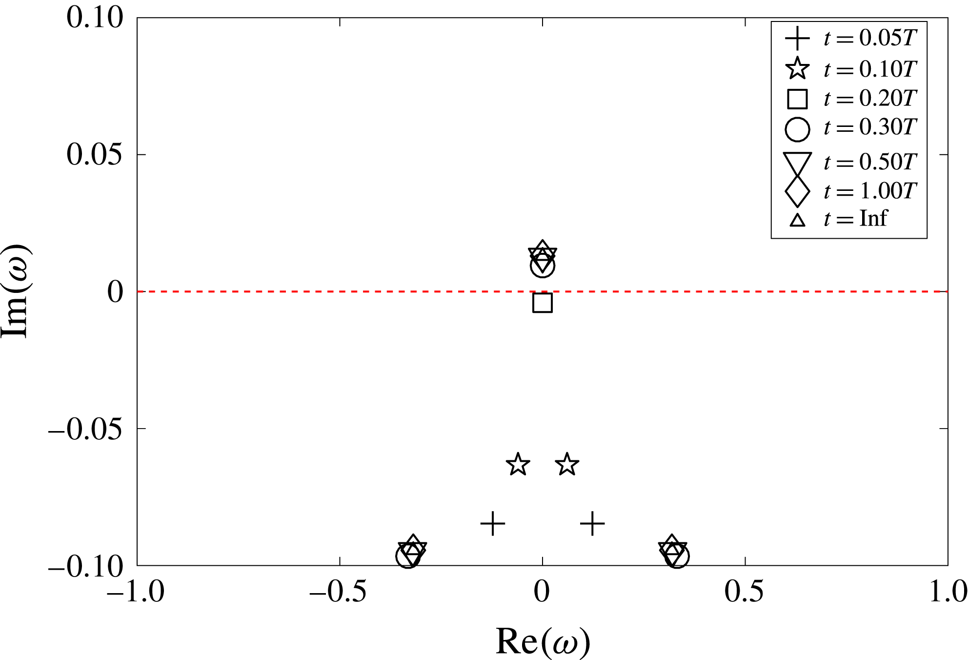
, which seems to be consistent with the description of the base flow given in § 5.2. In order to give a more quantitative explanation we solved a modified eigenvalue problem where the base flow is now given by the expression (5.1) for a collection of different times and with the same set of parameters as the reference experiment presented in figure 14. The results are presented in figure 16, where we report the eigenvalues of the most unstable mode focusing close to the transition region
 $\text{Im}(\unicode[STIX]{x1D714})=0$
. One remarks that no unstable eigenvalue is present for
 $t<0.2T_{\unicode[STIX]{x1D708}}$
while one unstable mode appears for
 $t\geqslant 0.3T_{\unicode[STIX]{x1D708}}$
, thus confirming that the base flow must be sufficiently established for the instability to develop. This result was confirmed by specific DNS where the initial condition is not the PC flow, but where the flow is initially at rest and the shear profile is progressively established through the no-slip boundaries. Also in this case the growth of perturbations is delayed to the moment when the shear profile has become almost constant. We then conclude that what we observe is associated with a constant shear PC profile.
Solutions of the modified eigenvalue problem for a base flow given by expression (5.1). Here we choose the same
 $Re$
,
 $Fr$
, and
 $U_{i}$
(i.e. the belt velocity at
 $t=0$
) as the reference experiment. The eigenvalues problem is solved for the combination
 $(k_{x},k_{z})$
, which is the most unstable according to linear analysis, and at seven different transient times shown by different symbols. The dashed line marks the limit for instability.

Besides determining the instability threshold in the
 $Re$
,
 $Fr$
space we also want to compare the shape of the mode selected in our experimental device with the unstable mode predicted by linear theory. If we focus again on the reference case described in figure 14, we note that both
 $k_{x}$
and
 $k_{z}$
are larger than the values predicted by the linear theory for the most unstable mode, and the perturbation is oscillatory in time while linear theory predicts a stationary mode. One can note that oscillations are quite regular and relatively slow, with a typical period
 $T=43\pm 3\unicode[STIX]{x1D70E}^{-1}$
, where the uncertainty is taken as the width at mid height of the peak in the average temporal spectrum. We recall that, according to linear analysis, oscillatory branches also exist (see figure 3) which appear at higher
 $Re$
number, typically
 $Re\gtrsim 2000$
. Interestingly the period associated with the first oscillating branch is always long; for example, with the
 $Fr$
of the reference experiment
 $N1$
and
 $Re=2500$
one has
 $T\sim 42\unicode[STIX]{x1D70E}^{-1}$
. Moreover, this branch happens at larger wavenumbers more compatible with the experimentally observed ones. In this scenario what we look at may be either a single propagative mode, for example of type (b), as is visible in the lower part of the spatio-temporal diagram (panel a of figure 14), or a standing wave generated by two counterpropagating modes of type (b) as is visible in the upper part of the same diagram. These elements suggest that, experimentally, the instability is activated close to the absolute threshold (i.e. where first stationary modes appear) predicted by linear analysis, but a different non-stationary mode is selected in the end.
In any case one should recall that our linear and experimental problems are different, thus unstable modes are not expected to share the same features. The major difference between the theoretical system and our experimental set-up is the finite size of the domain. In principle, to mimic periodic boundary conditions imposed in linear calculations, one wants to take the horizontal and vertical aspect ratio
 $D/d\gg 1$
and
 $H/d\gg 1$
, while our best realization (i.e. narrow gap) of this hypothesis was
 $D/d=5.7$
and
 $H/d=2.4$
. We observe that the impact of physical confinement is twofold. First, from the point of view of modal analysis only the wavelengths which fit in the domain may have a chance to develop. This was confirmed by periodic DNS that show no instability whenever the box size does not fit the spatial shape of unstable modes. We notice that the eigenvalue problem is solved by assigning an arbitrary value of
 $k_{x}$
and
 $k_{z}$
; thus when comparing to DNS and experiments one should retain that the (
 $k_{x},k_{z}$
) grid of figure 2 is coarsed grain, especially at low
 $k_{x}$
and
 $k_{z}$
. Thus the ideal constraints for the aspect ratio are
 $D/d\gg \unicode[STIX]{x1D706}_{x}$
and
 $H/d\gg \unicode[STIX]{x1D706}_{z}$
, where
 $\unicode[STIX]{x1D706}_{x}$
and
 $\unicode[STIX]{x1D706}_{z}$
are the non-dimensional wavelengths of the unstable mode we want to observe. A second problem appears in the streamwise direction because the streamlines must turn and close up when getting close to the walls that close the domain in the streamwise direction, as is clearly visible in the snapshot reported in figure 13. We mentioned before that this feature does not significantly modify the shape of the base flow in the bulk, but it may locally destabilize the flow (i.e. close to the corners) and successively affect the stability of the whole domain.
(a,c) Spatio-temporal diagram of the perturbation
 $u$
at the centre line
 $x=0$
,
 $y=0$
for the reference case
 $Re=969$
,
 $Fr=0.82$
for confined DNS (a) and the reference experiment (c). Spurious bulk oscillations are filtered from the experimental data. (b,d) Perturbation
 $u$
in the plane
 $y=0$
once the flow has become unstable for confined DNS (b) and the reference experiment (d). The red dashed rectangle indicates the area accessible to experimental measurements.

6.1 Simulations in a finite domain
In order to more closely investigate finite size effects, we perform new DNS where the computational domain is now closed in the streamwise direction by two solid walls with no-slip insulating boundary conditions, as sketched in figure 12(b), while boundary conditions remain periodic in the vertical direction. Note that compared with the periodic case discussed in § 4 the mesh is further refined close to the two additional streamwise boundaries, in order to properly solve for the boundary layers. In addition, the corners of the domain are now singular due to the incompatibility between the velocity imposed at the side boundaries and the fixed streamwise walls. This is naturally smoothed by viscosity but is nevertheless an inevitable source of vorticity. In figure 17(a,b) we report the results of a confined DNS which reproduces both the control parameters (
 $Fr$
,
 $Re$
) and the aspect ratio of the reference experiment illustrated in figure 14. For a direct comparison we report again the results of the reference experiment (c,d) already shown in figure 14, with the only difference that bulk oscillations are now filtered from the spatio-temporal diagram of
 $u$
at
 $x=y=0$
and the origin of time axis is shifted forward to
 $t=T_{\unicode[STIX]{x1D708}}/3$
, which is when we estimate that the PC flow is well established. One observes a strikingly good agreement between our DNS and experimental results on both the spatial and temporal shapes of the selected mode. Computing the temporal spectrum we find that the temporal frequency predicted by DNS is
 $T=50\pm 5\unicode[STIX]{x1D70E}^{-1}$
, which is compatible with the experimental one, while the consistency of spatial wavelengths is evident because in both cases an integer number of velocity maxima fit in the vertical midplane
 $y=0$
. Finally, we observe that as a whole the transition from the initial noise to the final nonlinear pattern takes almost the same time in DNS and in the experiment. As a summary, figure 17 indicates that we correctly isolated the crucial factor which possibly alters the selection of the unstable mode, that is the streamwise confinement. Incidentally we also report that additional DNS show that the form of the late nonlinear stage is quite sensitive to initial and boundary conditions. For example, slightly varying the box dimensions or the amount of initial noise the spatial shape of the selected mode is different and travelling waves or standing waves patterns can be alternatively present. To better investigate the role of streamwise boundaries we performed additional DNS with a non-stratified (
 $Fr=\infty$
) PC flow with exactly the same confined geometry with the same
 $Re$
number as the one we just described. We recall that perturbations do not grow when considering periodic boundary conditions at
 $Fr=\infty$
, as expected by the fact that the unstratified PC flow is linearly stable. One observes that vertical kinetic energy (black dashed line in figure 18) grows in an exponential way and in a shorter time compared to both the stratified DNS and experiment in figure 17, while the typical vertical length scale is larger. A similar pattern is also observed in the unstratified experiment as soon as
 $Re\gtrsim 300$
. A detailed investigation of the nature of this instability of a confined and unstratified PC flow is beyond the scope of the present work. Nevertheless, the shape of the flow at the corners suggests that it may locally destabilize via centrifugal instability, which will be studied in further investigations.
Vertical kinetic energy density
 $(\overline{w^{2}})^{1/2}$
as a function of time, for five different DNS. Black lines correspond to supercritical simulations (
 $Re=966$
) performed at
 $Fr=0.82$
(solid line),
 $Fr=\infty$
(dashed line) and
 $Fr=0.82$
with periodic boundary conditions in the streamwise direction (dash-dotted line). Red lines refer to subcritical simulations (
 $Re=629$
) performed at
 $Fr=0.53$
(solid line) and
 $Fr=\infty$
(dashed line). The thin black line corresponds to the growth of the most unstable mode at
 $Re=966$
,
 $Fr=0.82$
as predicted by the linear theory. Horizontal dashed lines highlight the saturation level of supercritical unstratified and stratified DNS, respectively.

We conclude that the presence of boundaries may destabilize the PC flow with or without the presence of stratification. Now, the careful reader will agree that even if DNS fully justify differences between the linear analysis and the observed experimental pattern we are left with a cumbersome question regarding the origin of the perturbation pattern observed in the confined and stratified configuration: does this pattern coincide with a boundary-induced modification of the linear instability, or rather with the pure hydrodynamic boundary-induced instability modified by the stratification?
The key to answer this resides in the same approach we followed with experiments: that is to detect if and when our flow abruptly changes when varying the control parameter
 $\unicode[STIX]{x1D70E}$
. We then consider further DNS which copy the parameters of another experiment of our reference series
 $N1$
where
 $Fr$
and
 $Re$
were 30 % smaller than the unstable case described in figure 14. At the same time we repeat unstratified simulations at such a lower value of the
 $Re$
number. We observe that the new unstratified case is almost unchanged while the subcritical stratified case shows a dramatic change. In this case, perturbations are significant only close to the boundaries, and no instability develops in the bulk. In figure 18 we report the time evolution of the vertical kinetic energy for all the streamwise-confined DNS we have discussed above, together with the one performed in a periodic domain. One observes that in the unstratified case (dashed line), perturbations rapidly grow and saturate at the same value independently of the
 $Re$
number. If we add stratification (solid lines), perturbation grows (black line) and saturates at the same value as the periodic simulation if the
 $Re$
number is beyond the threshold predicted by the linear analysis. Conversely perturbations are damped (red line) when the
 $Re$
number is below the threshold.
We have now enough elements to conclude that what we observe both in experiments and DNS (figure 17) is a signature of the linear instability of a PC flow, vertically stratified in density. In addition, we observe that streamwise boundaries are a source of instabilities and likely affect the features, or possibly just the selection, of the unstable mode which in the end shapes the observed pattern.
Incidentally we report that additional DNS were performed in a domain which is larger but still confined in the streamwise direction, in order to explore when finite-size effects become negligible and suitably design a larger experiment. Surprisingly we find that for a doubled size domain, the growth rate decreases and almost matches that of periodic simulations, but the instability disappears (we observe a pattern similar to the subcritical stratified case) when further increasing the streamwise domain (i.e. four times larger). With respect to this trend, the long computation time required to consider even larger domains prevents us being conclusive, and further studies will be necessary. The transition from the confined to the periodic case happens in a discontinuous way which needs to be further investigated. At this stage we speculate that streamwise boundaries may both introduce some forcing and inhibit the instability, perturbing the resonance of the waves supported by the flow. The horizontal aspect ratio possibly controls the mutual importance of these two effects in a non-trivial, non-monotonous way, thus explaining the observed scenario.
7 Conclusions
We performed the linear stability analysis of the PC flow for a stably stratified fluid with a constant density gradient orthogonal to the shear. The domain has rigid closed boundaries in the direction of the shear, and open periodic boundaries in both the vertical and streamwise directions. Unstable stationary modes are found at strikingly moderate Reynolds number
 $Re\geqslant 700$
and for a Froude number close to
 $1$
for non-vanishing horizontal and vertical wavenumbers with
 $k_{x}/k_{z}\sim 0.2$
. We then explore the stability of the flow in the
 $(Re,Fr)$
space. In the region we consider, the most unstable mode is always stationary and the growth rate remains relatively small, while the range of unstable
 $Fr$
numbers increases when increasing the
 $Re$
number. Moreover, the flow is unstable only to three-dimensional perturbations, i.e. only for
 $k_{x}$
,
 $k_{z}\neq 0$
. This result constitutes a fundamental difference from homogeneous shear flows, for which the Squire theorem prescribes that the most unstable mode should be two-dimensional. In the presence of stratification, the hyperbolic tangent profile (Deloncle et al.
Reference Deloncle, Chomaz and Billant2007) and the Kolmogorov flow (Lucas et al.
Reference Lucas, Caulfield and Kerswell2017) are also dominated by two-dimensional perturbations. On the contrary, three-dimensional perturbations appear on the stratified Taylor–Couette profile (Yavneh et al.
Reference Yavneh, McWilliams and Molemaker2001) as well as in parallel flows free from inflection points but with a vertical stratification, such as the boundary layer profile and the plane Poiseuille flow (Chen et al.
Reference Chen, Bai and Le Dizès2016). As in these latter cases, our three-dimensional instability appears close to
 $Fr=1$
, confirming the necessary coexistence of shear and stratification. The critical Reynolds number for the stratified PC flow turns to be at least two times smaller than for the boundary layer and slightly larger than for the Poiseuille flow.
Looking at the most unstable mode of the linear problem, vertical velocity and density perturbations develop close to the boundaries, which suggests that a crucial role may be played by lateral boundaries. Nevertheless, a comparable horizontal motion dominates in the mid vertical plane, and shows a vertically modulated pattern which is reminiscent of the deep equatorial currents, and staircase density layering in the Earth’s oceans (Dunkerton Reference Dunkerton1981; Dengler & Quadfasel Reference Dengler and Quadfasel2002; d’Orgeville et al. Reference d’Orgeville, Hua, Schopp and Bunge2004).
A mechanism was proposed to phenomenologically explain the onset of the instability as the one suggested by Satomura (Reference Satomura1981) adapted to the case of internal gravity waves, instead of shallow-water waves. In this picture, internal gravity waves are trapped close to the boundaries and Doppler shifted, thus allowing two counterpropagating waves to become stationary and mutually resonant. The shape of the unstable region in the wavenumber space and the appearance of discrete additional resonances are also fully captured by the model, thus supporting its relevance. An analogous mechanism was also invoked at the origin of strato-rotational instability both in the PC (Kushner et al. Reference Kushner, McIntyre and Shepherd1998; Vanneste & Yavneh Reference Vanneste and Yavneh2007) and the Taylor–Couette (Yavneh et al. Reference Yavneh, McWilliams and Molemaker2001; Park & Billant Reference Park and Billant2013) geometry. More generally this wave interaction process identifies a class of instability which is characteristic of shear flows (e.g. Baines & Mitsudera Reference Baines and Mitsudera1994).
The linear stability analysis was confirmed by DNS which reasonably well reproduce the spatial pattern and the growth rate. We report that no instability is observed when none of the unstable modes can properly fit in the domain. This confirms that the instability sharply selects the spatial pattern of the perturbation.
We analysed the experimental flow produced by a shearing device immersed in a tank filled with salty water, linearly stratified in density. We report that when the
 $Fr$
number is close to 1 and
 $Re\geqslant 10^{3}$
, velocity perturbations grow in an exponential way. Remarkably we observe that perturbations start to grow only when the PC profile is almost completely established. This was confirmed by ad hoc versions of the linear problem for a collection of transient profiles and by DNS which mimic the transient flow of experiments. We conclude that the observed instability is crucially associated with the shape of the shear, namely the PC profile.
Next, we explored the stability of the flow in the
 $(Re,Fr)$
space by varying the control parameter
 $\unicode[STIX]{x1D70E}$
, which is equivalent to moving along
 $Fr/Re=\text{const.}$
lines, for a few different values of
 $Fr/Re$
. For each series of experiments we observe that an abrupt increase in the perturbation amplitude occurs, when
 $\unicode[STIX]{x1D70E}$
is bigger than a threshold value
 $\unicode[STIX]{x1D70E}_{c}$
. When adding experimental data to the stability diagram predicted by the linear theory we find that the threshold contour indicated by experiments qualitatively matches the margin of the linearly unstable region. Also, close to the threshold, the velocity perturbation shows a well-organized pattern and is almost horizontal, which is in agreement with the solution of the linear problem. Nevertheless, the unstable mode slowly oscillates in time and appears at higher wavenumbers than the most unstable (stationary) mode indicated by the linear analysis. These two elements suggest that the mode selected in our experiment is not the most unstable of those predicted by linear analysis, or that these latter are possibly not the same when considering the finite-size experimental apparatus.
In any case we claim that the origin of the discrepancy relies on the critically low value of the horizontal aspect ratio of our experimental domain, which is necessarily bounded in the streamwise direction. The relevance of this hypothesis has been tested with complementary DNS where no-slip rigid boundaries are now implemented also in the streamwise direction. Remarkably, when copying the aspect ratio of our experiments we minutely reproduce the perturbation pattern observed in experiments. More generally, DNS show that streamwise confinement affects the stability of the flow irrespective of the
 $Fr$
number (i.e. also without stratification), which questions the link between the instability observed in experiment and that predicted by the linear analysis. We performed then DNS of a subcritical stratified experiment (i.e.
 $Re$
and
 $Fr$
below the critical value) and show that the instability disappears. We then acknowledge the unstable pattern observed in both experiments and DNS as a true signature of the linear instability of a PC flow vertically stratified in density.
Future studies are planned to more closely investigate which is the critical aspect ratio to recover quantitatively the results of linear theory and periodic DNS. With this aim new DNS will be performed in a larger domain, which will possibly indicate how to design a corresponding new set-up.
Quantitative measurements of the density field will be also performed in future experiments to quantify the density layering whose evidence was already available in our highest-Reynolds-number experiments in the form of regularly spaced optical distortion. Such measurements will possibly add clues to the comprehension of the diapycnal mixing in the presence of horizontal layering, as recently studied with experiments (Woods et al. Reference Woods, Caulfield, Landel and Kuesters2010; Oglethorpe et al. Reference Oglethorpe, Caulfield and Woods2013) and numerical simulations (Lucas & Caulfield Reference Lucas and Caulfield2017) in the case of the Taylor–Couette and Kolmogorov flows, respectively.
Acknowledgement
This work has been carried out thanks to the support of the A*MIDEX grant (ANR-11-IDEX-0001-02) funded by the French Government ‘Investissements d’Avenir’ programme.