1 Introduction
Buoyancy forces have a stabilizing effect on boundary layers when they act in the direction towards the wall. Such thermally stable flows are found in nocturnal atmospheric boundary layers where the air is warmer than the ground, and winds in the polar region where warm air flows over cold seas or ice. They may also be encountered in industrial settings such as plate heat exchangers. Stable stratification reduces turbulent mixing by inhibiting vertical transport, thereby significantly reducing heat and momentum transfer across the layer. With strong stable stratification the turbulent structure changes significantly, and additional flow features such as large-scale intermittency, gravity waves and Kelvin–Helmholtz instabilities become more important, invalidating many conventional boundary layer concepts (Mahrt Reference Mahrt1998, Reference Mahrt1999).
A number of experimental studies have examined the behaviour of thermally stable boundary layers (Arya Reference Arya1975; Ogawa et al. Reference Ogawa, Diosey, Uehara and Ueda1985; Ohya, Neff & Meroney Reference Ohya, Neff and Meroney1997; Ohya Reference Ohya2001). These investigations indicate a progressive dampening of turbulence with increasing stratification characterized by the bulk Richardson number,
 $$\begin{eqnarray}Ri_{\unicode[STIX]{x1D6FF}}=\frac{g\unicode[STIX]{x1D6FF}}{U_{\infty }^{2}}\frac{\unicode[STIX]{x0394}T}{T_{\infty }},\end{eqnarray}$$
where
 $g$
is the acceleration due to gravity,
 $\unicode[STIX]{x1D6FF}$
is the boundary layer thickness,
 $\unicode[STIX]{x0394}T$
is the temperature difference across the layer and
 $T_{\infty }$
and
 $U_{\infty }$
are the free stream temperature and velocity, respectively. For stable boundary layers, the Richardson number is positive.
More recently, Williams et al. (Reference Williams, Hohman, Van Buren and Smits2016) reported a parametric study of stably stratified boundary layers for momentum thickness Reynolds numbers of
 $600\leqslant Re_{\unicode[STIX]{x1D703}}\leqslant 2400$
and bulk Richardson numbers up to
 $Ri_{\unicode[STIX]{x1D6FF}}\approx 0.25$
. Here,
 $Re_{\unicode[STIX]{x1D703}}=U_{\infty }\unicode[STIX]{x1D703}/\unicode[STIX]{x1D708}_{\infty }$
,
 $\unicode[STIX]{x1D708}_{\infty }$
is the fluid kinematic viscosity at the free stream temperature, and the momentum thickness
 $\unicode[STIX]{x1D703}$
is defined according to
 $$\begin{eqnarray}\unicode[STIX]{x1D703}=\int _{0}^{\infty }\frac{\unicode[STIX]{x1D70C}U}{\unicode[STIX]{x1D70C}_{\infty }U_{\infty }}\left(1-\frac{U}{U_{\infty }}\right)\,\text{d}z\end{eqnarray}$$
(
 $U$
and
 $\unicode[STIX]{x1D70C}$
are the streamwise velocity and fluid density, respectively). It was found that for weak to moderate stability, the turbulent stress profiles scaled with the density weighted friction velocity
 $u_{\ast }$
, while the mean velocity profiles changed to a more laminar shape. Here,
 $u_{\ast }=\sqrt{\unicode[STIX]{x1D70C}/\unicode[STIX]{x1D70C}_{w}}u_{\unicode[STIX]{x1D70F}}$
, where
 $u_{\unicode[STIX]{x1D70F}}=\sqrt{\unicode[STIX]{x1D70F}_{w}/\unicode[STIX]{x1D70C}_{w}}$
,
 $\unicode[STIX]{x1D70F}_{w}$
is the wall stress, and
 $\unicode[STIX]{x1D70C}_{w}$
is the fluid density at the wall. The success in scaling the turbulent stresses with
 $u_{\ast }$
suggests little change in turbulent structure for moderate levels of stability. As in previous studies, the turbulent production was observed to collapse at higher Richardson numbers, resulting in patchy and highly intermittent turbulence.
Here, we are interested in the response of an initially neutral turbulent boundary layer to a change in wall temperature, leading to the progressive development of stable stratification. This type of flow is encountered, for example, in daytime summer offshore breezes where warm air flows from land onto a cooler ocean and in the flow over ice packs in the arctic. By studying such flows we hope to improve our understanding of these atmospheric processes.
In a more general context, the response of wall-bounded flows to perturbations in wall boundary conditions have been examined reasonably extensively (Smits & Wood Reference Smits and Wood1985; Garratt Reference Garratt1990), and examples include sudden changes in surface roughness (Antonia & Luxton Reference Antonia and Luxton1971, Reference Antonia and Luxton1972; Wood Reference Wood1982; Taylor, Mason & Bradley Reference Taylor, Mason and Bradley1987), blowing/suction (Simpson Reference Simpson1971; Squire, Thomas & Marriott Reference Squire, Thomas and Marriott1977), wall heat flux (Antonia, Danh & Prabhu Reference Antonia, Danh and Prabhu1977; Fedorovich et al.
Reference Fedorovich, Kaiser, Rau and Plate1996) and wall temperature (Johnson Reference Johnson1957; Ligrani & Moffat Reference Ligrani and Moffat1985; Mukerji, Eaton & Moffat Reference Mukerji, Eaton and Moffat2004). The latter four studies are perhaps most closely related to the present work, but in all cases the perturbations were ‘weak’ in that local similarity was preserved. Such weak step changes are commonly described in terms of the growth of an internal layer where the flow scales with the local wall shear, and an overlying external layer that continues to scale with the conditions upstream of the step. The extent of the internal layer is often seen to grow at a rate typical of a turbulent boundary layer, that is
 $\unicode[STIX]{x1D6FF}_{i}\sim \bar{x}^{0.8}$
, where
 $\bar{x}=x-x_{0}$
is the distance downstream of the step,
 $x$
is the distance measured from the origin of the boundary layer and
 $x_{0}$
is the distance from the boundary layer origin to the step. When
 $\bar{x}$
exceeds 10 to
 $20\unicode[STIX]{x1D6FF}$
, the internal layer has usually grown to the full extent of the boundary layer, although the relaxation distance for the turbulence is often much longer than that for the mean flow (Alving, Smits & Watmuff Reference Alving, Smits and Watmuff1990).
In terms of more severe step changes in wall temperature, Hara et al. (Reference Hara, Ohya, Uchida and Ohba2009) examined a destabilizing case, transitioning from a cooled to a heated floor. Also, Mahrt (Reference Mahrt2000) presented scaling arguments for the influence of surface heterogeneity of different types and sizes, and Stoll & Porté-Agel (Reference Stoll and Porté-Agel2009) performed large-eddy simulations of stably stratified atmospheric boundary layers over a surface with temperature transition patches. In these simulations, the effects of small patches (0.5 to
 $2\unicode[STIX]{x1D6FF}$
long) with a variety of temperature differences were studied in the very near field of the step change (
 $\bar{x}<4\unicode[STIX]{x1D6FF}$
), and the turbulent stresses were either amplified or damped within the internal layer, depending on whether the step change was destabilizing or stabilizing.
Here, we complement these simulations with an experimental study on the effects of imposing stable stratification on an initially neutral turbulent boundary layer. The surface is rough everywhere, and at the point where the flow encounters the change in wall temperature
 $Re_{\unicode[STIX]{x1D703}}=1280$
. The wall temperature differences produced Richardson numbers as high as
 $Ri_{\unicode[STIX]{x1D6FF}}=0.2$
. We find that the buoyancy time scale, that is, the inverse of the (bulk) Brunt–Väisälä frequency
 $N=\sqrt{(g/\unicode[STIX]{x1D6FF})\unicode[STIX]{x0394}T/T_{\infty }}$
, is an important parameter to describe the response of the turbulent stresses, and the rate of growth of the internal layer (
 $N$
may be interpreted as the frequency of oscillation of a fluid particle whose position is perturbed in the presence of a density gradient).
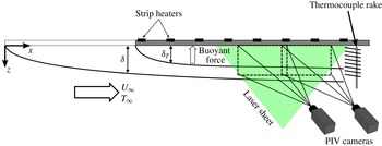
Schematic of the experimental set-up.

2 Experimental set-up
The boundary layer developed on the upper wall of a wind tunnel, as shown in figure 1. The wind tunnel is a suction type with a
 $1.2~\text{m}\times 0.9~\text{m}\times 5~\text{m}$
test section, operated at a fixed free stream velocity of
 $U_{\infty }=1.5~\text{m}~\text{s}^{-1}$
. The boundary layer was tripped using a 6.35 mm rod at the test section inlet and maintained with a square-weave wire mesh surface roughness having a wire mesh thickness of
 $k=4.1$
mm, which corresponds to
 $k^{+}=ku_{\unicode[STIX]{x1D70F}}/\unicode[STIX]{x1D708}_{w}\approx 24$
, and an equivalent sand grain roughness of
 $k_{s}^{+}=49$
, as defined by Nikuradse (Reference Nikuradse1933), where
 $$\begin{eqnarray}\unicode[STIX]{x0394}U^{+}=\frac{1}{\unicode[STIX]{x1D705}}\ln (k_{s}^{+})+B-8.5.\end{eqnarray}$$
Here,
 $\unicode[STIX]{x1D705}$
and
 $B$
are the slope and intercept of the logarithmic portion of the mean velocity profile; and the superscript
 $+$
denotes scaling using the friction velocity
 $u_{\unicode[STIX]{x1D70F}}$
and inner length scale
 $\unicode[STIX]{x1D708}_{w}/u_{\unicode[STIX]{x1D70F}}$
. The ratio of the boundary layer height to roughness height is
 $\unicode[STIX]{x1D6FF}/k=26$
. The boundary layer height at the beginning of our measurement region is
 $\unicode[STIX]{x1D6FF}_{0}=10.7$
cm, which is defined as the wall-normal location at which the local mean velocity peaks (the profiles displayed a small overshoot near the edge of the layer). All values correspond to the conditions at
 $x=2.44$
m for the neutral boundary layer (isothermal wall).
For
 $x\geqslant 2.44$
m (
 $\bar{x}\geqslant 0$
), the aluminium ceiling of the test section was heated using strip heating elements to generate the change in wall temperature. Because of the orientation of the wall, this heating leads to stable stratification. The boundary layer at the start of the heating had a height of
 $\unicode[STIX]{x1D6FF}_{0}=0.105$
m and
 $Re_{\unicode[STIX]{x1D703}}=1280$
. The wall temperature for
 $x>x_{0}$
was varied from
 $0\leqslant \unicode[STIX]{x0394}T\leqslant 120$
K, where
 $\unicode[STIX]{x0394}T=T_{w}-T_{\infty }$
(wall and free stream values denoted with subscripts
 $w$
and
 $\infty$
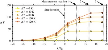
, respectively). The wall temperatures were monitored using multiple thermocouples installed on the test surface centerline, and the variation of temperature with downstream distance is shown in figure 2 for each of the test conditions. The uncertainty bars denote the standard deviation of the wall temperature at that location for over the entire experiment. We see that the change in temperature occurs over a distance of approximately 10 to
 $15\unicode[STIX]{x1D6FF}_{0}$
due to longitudinal heat conduction in the aluminium wall. Thus, at each measurement location we have the nominal and actual wall temperature differences,
 $\unicode[STIX]{x0394}T$
and
 $\unicode[STIX]{x0394}T_{a}$
respectively.
Wall temperature as it varies downstream for different wall temperatures. Temperature introduction and measurement locations are as marked.

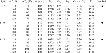
All test conditions are given in table 1. Here,
 $C_{f}=2\unicode[STIX]{x1D70F}_{w}/(\unicode[STIX]{x1D70C}_{\infty }U_{\infty }^{2})$
,
 $\unicode[STIX]{x1D6FF}$
is the local boundary layer thickness, and
 $Re_{\unicode[STIX]{x1D70F}}=\unicode[STIX]{x1D6FF}u_{\unicode[STIX]{x1D70F}}/\unicode[STIX]{x1D708}_{w}$
. At the furthest downstream station the bulk Richardson number
 $Ri_{\unicode[STIX]{x1D6FF}}$
reaches a maximum value of 0.2.
Test conditions at each downstream location.

We use two reference cases to describe the state of flow in the absence of the change in wall temperature. The first reference case is the state of the flow at the first measurement location with no heating (
 $\unicode[STIX]{x0394}T=0$
), referred to as the neutral case. The second reference case is the state of the flow with heating applied along the entire length of the test section, referred to as the developed stabilization case. The reference cases are taken from Williams (Reference Williams2014) and Williams et al. (Reference Williams, Hohman, Van Buren and Smits2016) who performed experiments using the same apparatus. Note that each wall temperature has a corresponding developed stabilization case.
Planar particle image velocimetry (PIV) measurements were taken at three downstream locations,
 $\bar{x}/\unicode[STIX]{x1D6FF}_{0}=5.7$
, 11.6 and 18.2 (marked in figure 2). A large field-of-view (window size
 $2.86\,\unicode[STIX]{x1D6FF}_{0}\times 1.5\,\unicode[STIX]{x1D6FF}_{0}$
) was achieved by using two overlapping PIV windows that were stitched together during processing. The LaVision PIV system used two 5.5 mega-pixel sCMOS cameras and a dual-pulsed 50 mJ Nd:YAG laser. Mineral oil smoke particles from a MAX 3000 MDG fog generator of approximately
 $1~\unicode[STIX]{x03BC}\text{m}$
in diameter were used for flow seeding. Further details on the PIV system and data processing techniques are given in Williams (Reference Williams2014) and Williams et al. (Reference Williams, Hohman, Van Buren and Smits2016). The random error of the PIV velocity measurements was estimated to be less than 1 % of the free stream velocity.
In the higher wall temperature cases the seeding of the flow field near the wall was more sparse as the seeding particles tended to evaporate. Hence, a wall-normal height is defined (
 $z_{10\,\%}$
) which is the location below which more than 10 % of the vectors were removed from the post-processing due to having a peak ratio less than 1.1, in conjunction with a normalized median filter (Westerweel & Scarano Reference Westerweel and Scarano2005) greater than two standard deviations of a
 $5\times 5$
neighbourhood. Below this height, the results are shown without symbols in the plots.
Temperature profiles were measured using a thermocouple rake. The rake spanned a wall-normal distance of 128.6 mm, with a thermocouple spacing that varied from a minimum of 4.8 mm near the wall, increasing to a maximum of 19 mm near the free stream. Calibrated macro photography was used to determine the wall-normal distance of the first thermocouple. All thermocouples were monitored using a National Instruments PCI-6229 board through LabView, accurate to
 $\pm 1\,^{\circ }\text{C}$
.
3 Results
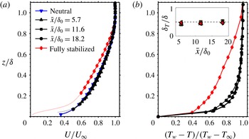
The mean velocity and temperature profiles are shown in figure 3. Whereas the mean velocity is almost unaffected by the change in wall temperature, the temperature layer is established very quickly, occupying approximately 50 % of the velocity boundary layer by the first measurement station (
 $\bar{x}/\unicode[STIX]{x1D6FF}_{0}=5.7$
). Further downstream the temperature layer grows very slowly, with some filling out of the profile evident at the most downstream measurement location for
 $\unicode[STIX]{x0394}T=120$
K. To find the skin friction coefficient
 $C_{f}$
, the wall stress
 $\unicode[STIX]{x1D70F}_{w}$
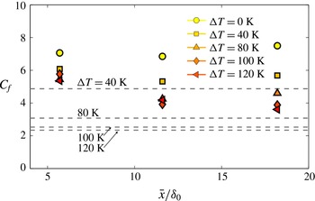
was approximated using the peak in the total stress distribution. The results, shown in figure 4, indicate that the skin friction is slow to respond to the change in buoyancy, but then gradually decreases further downstream by an amount that grows with increasing degree of stratification. Changing the reference density in the skin friction coefficient from
 $\unicode[STIX]{x1D70C}_{\infty }$
to
 $\unicode[STIX]{x1D70C}_{w}$
did little to change this trend.
(a) Mean velocity profiles, and (b) temperature profiles for
 $\unicode[STIX]{x0394}T=120$
K. The inset shows the ratio of the thermal boundary layer thickness
 $\unicode[STIX]{x1D6FF}_{T}$
to the velocity boundary layer thickness
 $\unicode[STIX]{x1D6FF}$
at the same location for each wall temperature (symbols for inset as in figure 2).

Skin friction coefficient variation. Dashed lines represent the skin friction coefficient for the developed stabilization cases.

The gradient Richardson number is a local estimate of the stratification effect (as opposed to the bulk Richardson number which is a mean value across the layer), and is defined according to
 $$\begin{eqnarray}Ri=\frac{g}{T_{\infty }}\frac{\unicode[STIX]{x2202}T/\unicode[STIX]{x2202}z}{(\unicode[STIX]{x2202}U/\unicode[STIX]{x2202}z)^{2}}.\end{eqnarray}$$
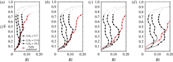
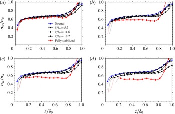
Figure 5 shows the gradient Richardson number profiles. The temperature and velocity gradients were computed as in Williams et al. (Reference Williams, Hohman, Van Buren and Smits2016). The data for
 $z/\unicode[STIX]{x1D6FF}_{0}\geqslant 0.75$
are indicated using a faint line because the gradients in this region become very small, and the accuracy of the data is questionable. We see that the trends are consistent across all levels of stratification. Near the wall, the gradient Richardson number increases almost linearly with wall-normal distance, with the extent of this linear variation increasing with increasing bulk stability and downstream distance. Beyond this region, a local peak in the gradient Richardson number develops, which is especially evident at the furthest downstream location. The peak is due to the temperature field reacting to the wall temperature change faster than the velocity field (see figure 3). The local gradient Richardson number exceeds the developed case near the wall for the strongest levels of stratification, indicating some non-equilibrium effects.
Gradient Richardson number profiles. (a)
 $\unicode[STIX]{x0394}T=40$
K; (b) 80 K, (c) 100 K, (d) 120 K. Data for
 $z/\unicode[STIX]{x1D6FF}_{0}\geqslant 0.75$
must be treated with caution due the small magnitudes of the mean gradients.

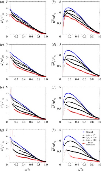
The stratification has a strong and immediate impact on the turbulence, as seen in figure 6. Here,
 $\overline{u^{2}}$
is the variance of the streamwise velocity component and
 $\overline{w^{2}}$
is the variance of the wall-normal velocity component, and we have normalized the data using
 $u_{\unicode[STIX]{x1D70F}0}$
, the friction velocity for the neutral case at
 $x=x_{0}$
. Williams et al. (Reference Williams, Hohman, Van Buren and Smits2016) found that for weak stratification the turbulence profiles scaled with the density weighted friction velocity
 $u_{\ast }$
. As suggested by our observations on the skin friction coefficient, this scaling would not be successful here, again indicating departures from equilibrium. The magnitude of the damping increases with the strength of the stratification, and even the smallest temperature difference produces noticeable changes in the stress profiles close to the location where the wall temperature changes, which was not seen in the mean velocity profiles. For
 $\unicode[STIX]{x0394}T\geqslant 80$
K, the impact of the change is evident over more than 60 % of the boundary layer for the streamwise and the wall-normal components.
Turbulence intensities normalized using the friction velocity for the neutral case. (a,c,e,g) Streamwise component. (b,d,f,h) Wall-normal component. (a,b)
 $\unicode[STIX]{x0394}T=40$
K; (c,d) 80 K, (e,f) 100 K, (g,h) 120 K.

To make a more quantitative comparison between the development of the two velocity components, we use the integral parameter
 $\unicode[STIX]{x1D706}$
, defined for the streamwise component by
 $$\begin{eqnarray}\unicode[STIX]{x1D706}_{u}=\frac{\displaystyle \int (\overline{u^{2}}-\overline{u^{2}}_{devstab})\,\text{d}z}{\displaystyle \int (\overline{u^{2}}_{neutral}-\overline{u^{2}}_{devstab})\,\text{d}z},\end{eqnarray}$$
with a similar definition of
 $\unicode[STIX]{x1D706}_{w}$
for the wall-normal component. This parameter represents a bulk measure of the turbulence development, where
 $\unicode[STIX]{x1D706}=0$
for the neutral case, and
 $\unicode[STIX]{x1D706}=1$
when the turbulence matches the developed stabilization case.
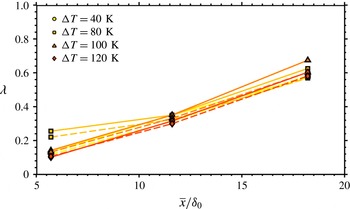
From figure 7 we see that
 $\unicode[STIX]{x1D706}$
grows approximately linearly with downstream distance, for this measurement domain and resolution, and the different levels of stability all display similar values. The first implication is that the bulk development is relatively unaffected by the magnitude of the change in wall temperature, and so for all cases the flow will reach the developed stabilization condition at a similar rate. The second implication is that the streamwise and wall-normal components of the velocity are developing at approximately the same rate. This is somewhat surprising because the buoyancy is expected to have a more direct impact on the wall-normal velocity fluctuations.
Bulk development parameter for the streamwise (——) and wall-normal (– – –) components.

To help interpret these trends, consider the transport equations for the streamwise and wall-normal components of the turbulence kinetic energy, and for the Reynolds shear stress
 $-\overline{uw}$
. We will neglect streamwise gradients of mean properties on the grounds that the flow evolves rather slowly (so that the usual boundary layer approximations continue to hold), and we will assume that departures from the Boussinesq approximation are not dynamically important. In the outer part of the boundary layer the transport terms are then small, and so for the streamwise component we have
 $$\begin{eqnarray}\frac{\text{D}\overline{u^{2}}}{\text{D}t}=-2\overline{uw}\frac{\unicode[STIX]{x2202}U}{\unicode[STIX]{x2202}z}+\frac{2}{\unicode[STIX]{x1D70C}}\overline{p^{\prime }\frac{\unicode[STIX]{x2202}u}{\unicode[STIX]{x2202}x}}-\unicode[STIX]{x1D716}_{u},\end{eqnarray}$$
where
 $p^{\prime }$
is the pressure fluctuation and
 $\unicode[STIX]{x1D716}_{u}$
is the streamwise velocity dissipation term. Similarly, we have for the wall-normal component (note that in our case gravity acts in the direction opposite to the direction of the temperature increase),
 $$\begin{eqnarray}\frac{\text{D}\overline{w^{2}}}{\text{D}t}=\frac{2}{\unicode[STIX]{x1D70C}}\overline{p^{\prime }\frac{\unicode[STIX]{x2202}w}{\unicode[STIX]{x2202}z}}+2\frac{g}{T_{0}}\overline{wT^{\prime }}-\unicode[STIX]{x1D716}_{w},\end{eqnarray}$$
where
 $T^{\prime }$
is the temperature fluctuation and
 $\unicode[STIX]{x1D716}_{w}$
is the wall-normal velocity dissipation term. For the Reynolds shear stress, only the production and the pressure strain terms are important in the outer layer, so
 $$\begin{eqnarray}\frac{\text{D}(-\overline{uw})}{\text{D}t}=\overline{w^{2}}\frac{\unicode[STIX]{x2202}U}{\text{d}z}+\frac{1}{\unicode[STIX]{x1D70C}}\left(\overline{p^{\prime }\frac{\unicode[STIX]{x2202}u}{\unicode[STIX]{x2202}z}}+\overline{p^{\prime }\frac{\unicode[STIX]{x2202}w}{\unicode[STIX]{x2202}x}}\right)+\frac{g}{T_{0}}\overline{uT^{\prime }}.\end{eqnarray}$$
We see that the wall-normal component loses energy through buoyancy-induced damping (
 $\overline{wT^{\prime }}<0$
). In turn, the reduction in
 $\overline{w^{2}}$
tends to reduce the production of
 $-\overline{uw}$
, with a further reduction through buoyancy (
 $\overline{uT^{\prime }}<0$
). Next, the streamwise component is reduced by a decrease in (positive) production. Hence, the buoyancy directly extracts energy from the wall-normal turbulence, but the streamwise turbulence is impacted mostly by the change in Reynolds shear stress. See also the related findings of Arya (Reference Arya1975) and Shah & Bou-Zeid (Reference Shah and Bou-Zeid2014). We note from figure 7 that the wall-normal component lags the streamwise component by a distance
 $O(\unicode[STIX]{x1D6FF})$
, which is typical of a large-eddy turnover time, and so this exchange among the components of the Reynolds stress through the pressure–strain term and buoyancy-driven damping occurs over a similar distance.
To explore this coupling further, we show the anisotropy ratio
 $\unicode[STIX]{x1D70E}_{w}/\unicode[STIX]{x1D70E}_{u}$
in figure 8, where
 $\unicode[STIX]{x1D70E}_{u}=\sqrt{\overline{u^{2}}}$
and similarly for
 $\unicode[STIX]{x1D70E}_{w}$
. The anisotropy ratio is almost constant across the boundary layer, and it demonstrates a very slow tendency toward the developed stabilization cases (especially for the higher temperature differences). Arya (Reference Arya1975) and Williams et al. (Reference Williams, Hohman, Van Buren and Smits2016) also noted that the anisotropy ratio for equilibrium boundary layers is relatively insensitive for weak to moderate levels of stability.
Anisotropy ratio profiles. (a)
 $\unicode[STIX]{x0394}T=40$
K; (b) 80 K, (c) 100 K, (d) 120 K.

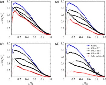
The Reynolds shear stress profiles are given in figure 9. As seen in the streamwise and wall-normal stresses, stability reduces the Reynolds shear stress, and the effects grow with downstream distance. On figure 9(d),
 $\unicode[STIX]{x1D701}$
denotes the wall-normal distance where the profiles match the neutral case. This point is taken to be a measure of the wall-normal extent of the impact of the change in wall temperature. The variation of
 $\unicode[STIX]{x1D701}$
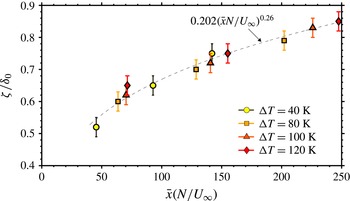
with downstream distance is shown in figure 10. The uncertainty bars are associated with the error in the estimate of
 $\unicode[STIX]{x1D701}$
which was determined from the standard deviation between five separate visual estimates. The results were found to collapse within the measurement domain when the streamwise distance
 $\bar{x}$
is normalized by a distance given by
 $U_{\infty }/N$
, where
 $N$
is the (bulk) Brunt–Väisälä frequency, so that we have a non-dimensional parameter
 $$\begin{eqnarray}\frac{\bar{x}N}{U_{\infty }}=\sqrt{\frac{\bar{x}^{2}}{\unicode[STIX]{x1D6FF}}\frac{g}{U_{\infty }^{2}}\frac{\unicode[STIX]{x0394}T}{T_{\infty }}}=\frac{\bar{x}}{\unicode[STIX]{x1D6FF}}\,\sqrt{Ri_{\unicode[STIX]{x1D6FF}}}.\end{eqnarray}$$
The variation of
 $\unicode[STIX]{x1D701}$
can be fitted by a power-law function
 $(\bar{x}N/U_{\infty })^{n}$
, where
 $n$
varies from approximately 0.15 to 0.35 for the range of virtual origins encompassed by the beginning and the end of the wall temperature rise. A smaller exponent will make the growth steeper for small values of
 $x$
, and less steep for large values, and so this internal layer grows more quickly close to the step and then more slowly downstream when compared to a typical growth rate of
 $x^{0.8}$
for an internal layer produced by a weak perturbation.
Our observation that the extent of the internal layer increases with the level of stable stratification is somewhat surprising. At first sight, we expect the opposite trend, in that thermal stability leads to decreased mixing (see Garratt (Reference Garratt1990) for discussion on internal boundary layer growth and Chung & Matheou (Reference Chung and Matheou2012) for a summary of this scaling in unbounded homogeneous stratified shear turbulence). Our data more closely follow the model of Venkatram (Reference Venkatram1977) for step changes in surface temperature or moisture which is most often applied to unstable and approximately neutrally stratified flows and suggests that the internal layer growth increases with the strength of the disturbance. However, Williams et al. (Reference Williams, Hohman, Van Buren and Smits2016) observed that decreases in mixing for weak to moderate levels of stability were proportional to reductions in the wall shear stress and continued to follow the scaling laws for neutrally stratified flows (when accounting for changes in fluid density). The results from the present study appears to fall in the same weak to moderate stability regime, as indicated by the insensitivity of the anisotropy parameter to the change in wall temperature. It seems plausible, therefore, that the growth of internal layer observed here more closely follows trends seen in neutrally stratified flows since the mixing processes seem to be largely unchanged by the presence of stability. It should also be noted that our scaling is based on an outer layer measurement, whereas atmospheric measurements are limited to the inner layer.
Reynolds shear stress profiles. (a)
 $\unicode[STIX]{x0394}T=40$
K; (b) 80 K, (c) 100 K, (d) 120 K. Circles on (d) mark the wall-normal extent where the boundary layer scales with the upstream boundary condition.

Wall-normal extent of the impact of the change in stable stratification on the Reynolds shear stress.

4 Conclusions
A thermally stable stratified boundary layer subject to a change in wall temperature was examined for a range of temperatures. The mean velocity profile showed little change over the range of streamwise location studied, but the temperature layer was established quickly but then showed little evolution downstream. This evolution was reflected in the local gradient Richardson number distributions, with localized peaks appearing in the profile that moved away from the wall and diffused downstream. This peak is likely due to the fast evolution of the mean temperature profile relative to the velocity profile.
The streamwise and wall-normal components of the turbulent stress were damped at approximately equal rates by the effects of buoyancy, indicating a strong coupling between the wall-normal and streamwise components on a time scale typical of a large-eddy turnover time (
 $O(\unicode[STIX]{x1D6FF}/U_{\infty })$
). The local response, as measured by bulk development parameters, grew linearly downstream at about the same rate for both components, invariant of the level of stability, suggesting that the rate of response was largely independent of the magnitude of the step change. The Reynolds shear stress was used to identify the internal layer, and the growth of this inner layer approximately followed a
 $(\bar{x}N/U_{\infty })^{0.26}$
power law where
 $N$
is the bulk Brunt–Väisälä frequency. Hence, it appears that the local turbulence response is on a scale of the eddy turnover time, and the asymptotic response is governed by the Brunt–Väisälä frequency. The ratio of these time scales is simply given by
 $N\unicode[STIX]{x1D6FF}/U_{\infty }$
, known as the inverse Froude number, that is,
 $\sqrt{Ri_{\unicode[STIX]{x1D6FF}}}$
.
Acknowledgement
This work was supported in part by the Cooperative Institute for Climate Science (CICS) at Princeton University.