1. Introduction
After peaking in the 1970s, the inflation rate in the U.S. remained low and stable for about four decades. As a result, monetary policy enjoyed unprecedented credibility and managed to maintain expectations firmly anchored. The most notable challenges during this period were, in fact, related to the possibility of inflation remaining too long below, rather than above, target, prompting central banks to implement expansionary policies to sustain inflation expectations. Conditions changed, however, in the aftermath of the COVID-19 pandemic, leading to the somewhat unexpected return of high inflation in 2021–2022, which reached levels last seen in 1981.
Different factors have been suggested to explain the rise in inflation. Fundamentally, price increases originated from a relatively rapid economic recovery after the pandemic-driven recession, combined with bottlenecks in established supply chains.Footnote 1 Under these conditions, the strong demand pressure couldn’t be met by a corresponding expansion in supply. Moreover, as Reis (Reference Reis2023) notes, inflation also resulted from more subtle factors, such as real-time misperceptions of shocks, initially perceived as more temporary than they proved to be, leading to overly expansionary monetary and fiscal policy stances. Past policy successes also led to an overreliance on the power of central banks’ credibility and a disregard for possible spillovers of inflationary shocks to inflation expectations, which were believed unlikely to become unmoored.
The main objective of this paper is to investigate the post-pandemic rise and fall of inflation within the context of a longer historical sample and through the lens of a New Keynesian model with shifting behavioral and heterogeneous expectations. Compared to existing research, the paper puts expectations at the forefront of the analysis to understand the behavior of inflation during the COVID years. The hypothesis is that the initial shocks gradually led to the partial unanchoring of expectations, which, in turn, exacerbated the increase in realized inflation and potentially hindered the effectiveness of monetary policy.
The paper revisits the history of inflation, business cycles, and monetary policy, as well as the corresponding expectations, in the period from the mid-1960s until 2024. The economic framework used is an otherwise standard New Keynesian model, as it remains a leading tool to understand the interplay between macroeconomic variables and monetary policy decisions. The benchmark framework, however, typically imposes two strong assumptions: the first is that agents form model-consistent rational expectations. In their decisions, they derive mathematical expectations that are conditioned on a model of the economy that happens to be the correct one; at the same time, they know the values of preference, technology, and policy parameters, as well as the distributions of the shocks. The second is that all agents have homogeneous expectations: there is no scope for disagreement or for reevaluating one’s views in such an economic environment.
This paper departs from these two conventional assumptions by including behavioral elements in the formation of expectations and by incorporating heterogeneous views about the direction of the economy. This extension aims to better capture the real-time interactions among exogenous shocks, policy reactions, and the potential anchoring or unanchoring of expectations. The conventional assumption of full information, homogeneous, rational expectations, in fact, is less suited to study agents’ behavior during unprecedented times, such as the COVID pandemic: it would imply that agents maintain full understanding about the workings of the economy, that they have full knowledge about exogenous shocks and their effects, about the effects of counteracting policies, and that they all share the same prediction model with no role for disagreement. On the other hand, adaptive learning and heterogeneous expectations provide natural frameworks to account for shifts in beliefs in response to new information and for divergences in opinion.
Here, different shares of agents in the economy are allowed to form expectations based on alternative perceptions regarding future economic variables. First, a share of agents form forecasts based on the perception that inflation, output, and interest rates will rapidly revert to their long-run values. They believe that the economy reaches steady state rather quickly, and they are trying to learn about such steady-state levels. A second share of agents forms forecasts based on a perceived model that resembles the Minimum State Variable (MSV) solution under rational expectations, which therefore includes all the relevant state variables that matter for economic dynamics (their model is thus correctly specified). This group forms expectations that present the smallest deviation from rational expectations, but they can still remain arbitrarily far from the Rational Expectations Equilibrium; unlike under RE, they do not have full knowledge of the model’s parameters, and, therefore, they need to learn the relevant coefficients over time. A third share of agents, finally, use an under-specified model, which captures trend-following, adaptive or extrapolative, behavior. These agents are backward-looking: they observe rising inflation, for example, and they lean on past inflation rates to infer how persistent above-target fluctuations can be expected to be.
Under each view of the world, agents are allowed to learn over time the parameters of their perceived model. In the mean reversion view, they learn about long-run values, or steady states. In the trend-following case, they learn about both intercepts and persistence (autoregressive coefficients). And in the correctly specified MSV model, they learn about the full set of reduced-form coefficients that would enter the model solution under rational expectations, including the sensitivity of endogenous variables to disturbances (observed by agents in this latter case as they would be under RE).
Households and firms are not forced to maintain the same beliefs indefinitely. They can shift among different views, depending on the past forecasting performance of the different perceived models. Learning about different models of the economy is implemented using sets of forecast encompassing regressions and allowing agents to revise the weights of the three different models based on past data. Learning both within and between models is modeled according to a constant-gain learning approach.
The macroeconomic model is estimated using Bayesian methods to fit realized macroeconomic variables but also to fit data on expectations about output, inflation, and interest rates, which are also treated as observables.
The results show that models used to form expectations indeed switch during the pandemic. The share of agents with forecasting models consistent with rapid mean reversion falls to its lowest historical level. This model is replaced by a much larger share of agents who adopt a trend-following approach. Agents also update their beliefs, learning that the persistence of inflation is much higher than perceived only a few quarters before. As a result of these expectation shifts, aggregate inflation expectations become much more reactive to inflationary shocks. The anchoring of expectations becomes shakier, leading to a reduced effectiveness of monetary policy efforts.
It should be noticed that these shifts do not materialize immediately at the onset of the pandemic. In the first quarters, with COVID positivity and death rates at their highest, inflation initially falls below target and then slowly rises. Inflation expectations, however, remain fairly stable. Starting in 2021, the observed inflation rate rises more significantly and the increases become persistent. At that point, expectations become less anchored: they rise, slowly at first, then more rapidly, and they continue to rise when inflation has already reversed direction. It’s around that point that agents had turned away from their mean reversion views and started to adopt trend-following expectations, characterized by a consistent update in the perceived inflation persistence. In addition to changes in first moments, the dispersion of both inflation expectations and monetary policy expectations increases in late 2022 and 2023.
Related literature. An extensive literature has analyzed the evolution of inflation over the post-war period (King and Watson, Reference King and Watson1994, Cogley and Sargent, Reference Cogley and Sargent2001, Lubik and Schorfheide, Reference Lubik and Schorfheide2004, Sargent et al., Reference Sargent, Williams and Zha2006, among many others). This paper contributes to this line of work by singling out the role that deviations from full-information rational expectations, behavioral elements, and shifts in perceived models of expectation formation play. In this respect, the paper is an example of macroeconomics without the Rational Expectations Hypothesis, to use the terminology in Woodford (Reference Woodford2013).
The emphasis on expectation heterogeneity follows works by Branch and McGough (Reference Branch and McGough2009, Reference Branch, McGough, Branch and McGough2018), who derive an Heterogeneous Expectations New Keynesian (HENK) model. In their case, they allow for two types of expectations: conventional rational expectations or backward-looking adaptive expectations. My choice here is different: all agents can form subjective expectations, but from different learning models, corresponding to different forecasting views. Beqiraj et al. (Reference Beqiraj, Di Bartolomeo and Serpieri2019), Massaro (Reference Massaro2013), Elias (Reference Elias2022), and Ilabaca and Milani (Reference Ilabaca and Milani2021) provide different examples of estimated HENK models.Footnote 2
The paper, more generally, adds to the literature on adaptive learning in macroeconomics and, more specifically, to the use of learning to understand the history of inflation. Sargent (Reference Sargent1999), Primiceri (Reference Primiceri2006), and Orphanides and Williams (Reference Orphanides and Williams2005) show how central bank learning helps explain policy mistakes that led to high inflation in the 1970s. Evans and Honkapohja (Reference Evans and Honkapohja1999, Reference Evans and Honkapohja2009) provide comprehensive reviews of the adaptive learning approach to expectation formation. While most papers introduce learning in a representative agent, homogeneous expectations, context, this work extends the approach to allow for heterogeneity in expectations.
A recent paper by Gáti (Reference Gáti2023) uses a learning model with an endogenous gain to model the anchoring and unanchoring of expectations and to study the optimal monetary policy response. With respect to Gáti, the unanchoring in this paper is similarly endogenous, but it is due to perceived model shifts rather than to shifts in the gain.Footnote 3 A closer approach is used in Fischer (Reference Fischer2022): the paper derives an endogenous measure of expectations anchoring in an estimated New Keynesian model with forecast switching, with the aim of studying the appropriate monetary policy response. The shifts are modeled following the approach by Brock and Hommes (Reference Brock and Hommes1997). My paper uses a different approach to model heterogeneous expectations, one that treats learning within and between models symmetrically, and it focuses on the behavior of inflation post-2020.
The paper has also points of contact with works that study the endogenous transition between different inflation equilibria, for example, between target-inflation and deflationary equilibria. Hecker and Wolters (Reference Hecker and Wolters2024) estimate a nonlinear model that allows such switches. Expectations in their paper become a weighted average of the corresponding expectations under the two regimes, with weights based on the recent forecasting performance. In this way, changes in the relative model shares can capture the unanchoring of expectations.
Finally, a number of papers have started to discuss and test hypotheses about the surge of inflation after COVID. Reis (Reference Reis2023) discusses factors that led policymakers to initially downplay the relevance of inflationary pressures. Various studies evaluate the relative importance of demand versus supply shocks in the run-up of inflation (e.g., Giannone and Primiceri, Reference Giannone and Primiceri2024, Bai et al., Reference Bai, Fernández-Villaverde, Li and Zanetti2024, Di Giovanni et al., Reference Di Giovanni, Kalemli-Özcan, Silva and Yildirim2023, Arias et al., Reference Arias, Rubio-Ramírez and Shin2025). Harding et al. (Reference Harding, Lindé and Trabandt2023) resort to a nonlinear Phillips curve that steepens when inflationary pressures emerge. Ball et al. (Reference Ball, Leigh and Mishra2022) examine the role of tightening labor markets and energy prices. The current paper provides some additional evidence concerning this period, identifying the contribution of expectational shifts, but with an analysis that inserts the post-COVID episode in the context of a longer sample. Schmitt-Grohe’ and Uribe (Reference Schmitt-Grohé and Uribe2022) use an even longer sample (1900–2021) to estimate changes in the permanent component of inflation between 2019 and 2021.
The paper is organized as follows. Section 2 presents the New Keynesian model with the addition of behavioral elements. Section 3 discusses the data and the Bayesian estimation of the model. Section 4 illustrates the empirical results from the structural estimation; the robustness of the results is examined in Section 5. Finally, Section 6 reports the conclusions.
2. New Keynesian model with heterogeneous behavioral expectations
I assume that the economy can be summarized by a prototypical New Keynesian model, as in Woodford (Reference Woodford2003). The main novelty lies in the formation of expectations. First, in contrast to the benchmark New Keynesian specification, which assumes homogeneous expectations for all agents in the economy, I allow here for heterogeneous expectations. Economic agents may form expectations from different perceived models of the economy. Moreover, the framework does not impose the assumption of rational expectations on the agents. Households and firms have their own views about the economy, which may be correctly specified or not, but they are also allowed to learn about the economy in response to historical data and to revise their beliefs.
The loglinearized equations that describe the economy in the New Keynesian model are as follows
 \begin{align} y_{t} &= \widehat {E}_{t}y_{t+1}-\sigma \left ( i_{t}-\widehat {E}_{t}\pi _{t+1}-r_{t}^{n}\right ) \end{align}
 \begin{align} \pi _{t} &= \beta \widehat {E}_{t}\pi _{t+1}+\kappa y_{t}+u_{t} \end{align}
 \begin{align} i_{t} &= \rho i_{t-1}+(1-\rho ) [\chi _{\pi }\pi _{t}+\chi _{y}y_{t} ]+\varepsilon _{t}, \end{align}
 \begin{align} r_{t}^{n} &= \rho _{r} r_{t-1}^{n}+\nu _{t}^{r}, \end{align}
 \begin{align} u_{t} &= \rho _{u} u_{t-1}+\nu _{t}^{u}, \end{align}
where
 $y_{t}$
denotes output,
 $\pi _{t}$
denotes inflation,
 $i_{t}$
denotes the nominal interest rate, and
 $r_{t}^{n}$
,
 $u_{t}$
denote the natural rate and the cost-push disturbances. Equation (1) denotes a log-linearized Euler equation, which arises from households’ optimal consumption and saving decisions. Current output is a function of expected output and of the ex-ante real interest rate (the nominal rate minus expected one-period-ahead inflation) in deviation from the time-varying exogenous natural rate. Equation (2) represents the New Keynesian Phillips curve. Inflation fluctuations are driven by fluctuations in expected inflation, real activity, and markup, or cost-push, shocks. Finally, monetary policy is characterized by a Taylor rule, expressed by equation (3). The central bank revises its policy rate, given by a short-term nominal interest rate, in response to changes in inflation and output. Disturbances
 $r_{t}^{n}$
and
 $u_{t}$
evolve as AR(1), whereas monetary policy innovations
 $\varepsilon _{t}$
are assumed to be i.i.d. The parameter
 $\kappa$
is a composite parameter, which depends inversely on the degree of price stickiness in the economy, measured by the Calvo probability
 $\alpha$
:
 $\kappa \equiv \frac {(1-\alpha )(1-\alpha \beta )}{\alpha }(\psi +\sigma ^{-1})$
. The parameter
 $\sigma$
denotes the intertemporal elasticity of substitution,
 $\psi$
the inverse Frisch elasticity of labor supply, and
 $\beta$
the household’s discount factor. The Taylor rule coefficients
 $\rho$
,
 $\chi _{\pi }$
, and
 $\chi _{y}$
denote the degree of interest-rate smoothing and the reaction coefficients to inflation and output.
Expectations in the model are denoted by
 $\widehat {E}_{t}$
. They can differ from the mathematical expectation operator
 $E_{t}$
, conditional on the correct model of the economy, which is commonly assumed under rational expectations. Expectations are heterogeneous and are a weighted average of expectations based on three different perceived models:
 \begin{align*} \widehat {E}_{t}\begin{bmatrix} y_{t+1}\\ \pi _{t+1}\\ i_{t+1} \end{bmatrix} = \widehat {\omega }_{t}^{ss} \, \widehat {E}_{t}^{ss}\begin{bmatrix} y_{t+1}\\ \pi _{t+1}\\ i_{t+1} \end{bmatrix}+\widehat {\omega }_{t}^{ar} \, \widehat {E}_{t}^{ar}\begin{bmatrix} y_{t+1}\\ \pi _{t+1}\\ i_{t+1} \end{bmatrix}+\widehat {\omega }_{t}^{msv} \, \widehat {E}_{t}^{msv}\begin{bmatrix} y_{t+1}\\ \pi _{t+1}\\ i_{t+1} \end{bmatrix} \end{align*}
The three perceived models are meant to represent three main views about the direction of the economy or alternative attitudes in forecasting.
The first model captures the behavior of forecasters who believe that the economy will quickly converge back to steady state. The Perceived Law of Motion (PLM) is given by
 \begin{align*} & \begin{bmatrix} y_{t}\\ \pi _{t}\\ i_{t} \end{bmatrix} = \widehat {a}_{t}^{\, ss} + \epsilon _{t} \end{align*}
where
 $\widehat {a}_{t}^{\, ss}$
is a 3×1 vector of perceived intercepts. When they form expectations, these agents believe that output, inflation, and interest rates will return to their long-run, steady-state levels by the following period. But such steady states are not full knowledge in the economy. Therefore, the agents still learn about steady-state levels and may revise their perceptions over time, for example, by revising up their views about the long-run trend growth rate, long-run inflation, and interest rates, based on historical data.
The second perceived model aims to capture the behavior of agents that display more backward-looking, trend-following behavior in the formation of their forecasts. Their PLM is as follows:
 \begin{align*} & \begin{bmatrix} y_{t}\\ \pi _{t}\\ i_{t} \end{bmatrix} = \widehat {a}_{t}^{\, ar} + \widehat {b}_{t}^{ar} \begin{bmatrix} y_{t-1}\\ \pi _{t-1}\\ i_{t-1} \end{bmatrix} + \epsilon _{t} \end{align*}
where
 $\widehat {a}_{t}^{\, ar}$
is again a vector of perceived intercepts and
 $\widehat {b}_{t}^{ar}$
is a matrix of AR coefficients as follows:
 $ \widehat {b}_{t}^{ar} = \begin{bmatrix} b_{yy,t} & 0 & 0 \\ 0 & b_{\pi \pi ,t} & 0\\ 0 & 0 & b_{ii,t} \end{bmatrix}. $
Their model allows for an intercept and a lagged dependent variable, and it resembles AR(1) regressions. Therefore, they learn both about long-run values and persistence of economic variables.Footnote
4
The perceived persistence of different variables can change over time: when the
 $b_{\cdot ,t}$
coefficients are below one, their expectations are usually described as adaptive; if they rise above one, they are labeled as extrapolative and may be particularly destabilizing for the economy.
For the third PLM, agents use the MSV solution of the model under RE:
 \begin{align*} & \begin{bmatrix} y_{t}\\ \pi _{t}\\ i_{t} \end{bmatrix} = \widehat {a}_{t}^{\, msv} + \widehat {b}_{t}^{msv} \begin{bmatrix} y_{t-1}\\ \pi _{t-1}\\ i_{t-1} \end{bmatrix}+ \widehat {c}_{t}^{\, msv} \begin{bmatrix} r_{t}^{n}\\ u_{t} \end{bmatrix} + \epsilon _{t} \end{align*}
Therefore, beliefs under the third PLM are closer to those in the rational expectations case: agents use a correctly specified model, i.e., a model that includes all the correct state variables in the MSV solution. The main deviation from rational expectations is that agents do not know all the parameters in the model, and, therefore, they need to learn about the reduced-form coefficients of the economy over time, as typical in models with adaptive learning. They learn about intercepts
 $\widehat {a}_{t}^{\, msv}$
, dynamic coefficients in
 $\widehat {b}_{t}^{msv}$
, and they learn via their estimates
 $\widehat {c}_{t}^{\, msv}$
about the effects of disturbances
 $r_{t}^{n}$
and
 $u_{t}$
, since those also enter the MSV solution.
In all cases, agents learn about their relevant coefficients
 $a_{t},b_{t},c_{t}$
, collected into a matrix
 $\widehat {\mathbf{\phi }}_{t}$
, for their PLM according to a constant-gain algorithm:
 \begin{align*} & \widehat {\mathbf{\phi }}_{t} =\widehat {\mathbf{\phi }}_{t-1}+\overline { \mathbf{g}}_{j}R_{t}^{-1}X_{t}(Z_{t}-\widehat {\mathbf{\phi }}_{t-1}^{ \ \prime } X_{t})^{\prime }, \\ & R_{t} =R_{t-1}+\overline {\mathbf{g}}_{j}(X_{t}X_{t}^{\prime }-R_{t-1}), \end{align*}
where
 $\widehat {\phi }_{t}=[a_{t}^{\, j},b_{t}^{\, j},c_{t}^{\, j}]^{\prime }$
,
 $Z_{t}=[y_{t},\pi _{t},i_{t},r_{t}^{n}, u_{t}]'$
, and
 $j = ss, ar, msv$
. The first expression governs learning about coefficients: agents’ beliefs are revised in the direction of the most recent forecast errors, with a sensitivity that depends on the size of the constant gain coefficient
 $\overline {\mathbf{g}}_{j}$
. The second expression characterizes the updating of the associated precision matrix
 $R_{t}$
, the inverse of the regressors’ variance-covariance matrix. The constant gains are allowed to differ across models: agents who use a model with only an intercept as regressor, may, in principle, update their beliefs at different speed compared with agents who learn the coefficients in a fully specified model with multiple regressors.
In addition to learning about coefficients within their chosen models, agents may also switch forecasting strategies over time. They don’t have to remain attached to the same views forever. Agents can choose to put more weight on a different model if its past forecasting performance improves compared with the alternatives. To describe shifts among models, I assume that agents adopt the following forecast encompassing regression
 \begin{align*} Z_{t} = \omega _{t}^{ss}\, {\widehat {E}}_{t-1}^{ss} Z_{t}+{\omega _{t}^{ar}}\, {\widehat {E}}_{t-1}^{ar} Z_{t}+\omega _{t}^{msv} \, {\widehat {E}}_{t-1}^{msv} Z_{t}+\nu _{t}. \end{align*}
Agents revise the weights of different forecasting models based on constant gain updating equations, as before:
 \begin{align*} & \widehat {\mathbf{\omega }}_{t} =\widehat {\mathbf{\omega }}_{t-1}+\overline {\mathbf{g}}_{m}R_{\omega ,t}^{-1}X_{t}(Z_{t}-\widehat {\mathbf{\omega }}_{t-1}^{ \ \prime } X_{t})^{\prime }, \\ & R_{\omega ,t} =R_{\omega ,t-1}+\overline {\mathbf{g}}_{m}(X_{t}X_{t}^{\prime }-R_{\omega ,t-1}), \end{align*}
The constant gain coefficient related to model learning
 $\overline {\mathbf{g}}_{m}$
can be different from the ones used to learn coefficients within specific models.
An alternative way to introduce model switching would be to follow the predictor switching approach theorized by Brock and Hommes (Reference Brock and Hommes1997). The main advantage of the encompassing approach is its simplicity, as well as the symmetry between learning within and across models.
3. Estimation
3.1 Observations
The model is estimated to match both realized macroeconomic variables and the corresponding, observed, expectations.Footnote 5
The observation equations relate the endogenous and expectational variables in the model to observed series as follows:
 \begin{align*} & \begin{bmatrix} Real \ Time \ Real \ Output \ Growth_{t}\\ Real \ Time \ Inflation_{t}\\ Federal \ Funds \ Rate_{t} \\ Expected \ Real \ Output \ Growth_{t+1} \\ Expected \ Inflation_{t+1} \\ Expected \ Federal \ Funds \ Rate_{t+1} \\ \end{bmatrix} = \begin{bmatrix} \delta \\ \pi ^{*}\\ \pi ^{*}+r^{*} \\ \delta \\ \pi ^{*}\\ \pi ^{*}+r^{*} \end{bmatrix}+ \begin{bmatrix} y_{t}-y_{t-1}\\ \pi _{t}\\ i_{t} \\ \widehat {E}_{t} \left [y_{t+1}-y_{t}\right ]\\ \widehat {E}_{t}\pi _{t+1}\\ \widehat {E}_{t}i_{t+1} \end{bmatrix} + \begin{bmatrix} 0 \\ 0\\ 0 \\ me_{t}^{Ey} \\ me_{t}^{E\pi }\\ me_{t}^{Ei} \end{bmatrix} \end{align*}
The parameter
 $\delta$
denotes the long-term trend in real GDP growth;
 $\pi ^{*}$
and
 $r^{*}$
denote the steady-state levels of inflation and real interest rates. Those are simply fixed at their sample means. I assume the same long-run values for realized variables and expectations. This isn’t restrictive, since agents are still allowed to over- or underestimate steady-state values through the
 $a_{t}$
intercepts in their learning models.Footnote
6
Data on expectations are obtained from the Survey of Professional Forecasters, maintained by the Federal Reserve Bank of Philadelphia. I use data on one-period-ahead expectations about Real GDP growth and GDP Price Deflator inflation. The Philadelphia Fed’s website publishes, in correspondence of each expectation series, the real-time vintage for the macroeconomic variable that is being forecast. I choose the first vintage for real-time data on GDP growth and inflation, considered as realized variables in the estimation. As a measure of monetary policy, I follow the literature in using the Federal Funds rate. I exploit the expectations theory to derive a measure of expected policy rates for the one-quarter-ahead horizon: specifically, I use the three-month interbank rate, obtained from FRED. The three-month rate should provide a measure of the expected average Federal Funds rate over the next quarter, after controlling for a possible, almost trivial, term premium. An alternative would be to replace the Federal Funds rate with the three-month Treasury bill rate, since SPF forecasts for three-month T-bill rates are available starting from 1981:Q3. But the choice of the Federal Funds rate and three-month interbank rate allows me to use a longer sample that also includes the run-up of inflation in the late 1960s into the 1970s.
The estimation sample starts from 1965 for real-time data, with the first observations on expectations available from 1968:IV, and it ends on 2024:II. The data are quarterly. The likelihood is computed from 1965, therefore allowing for missing data and a different set of observation equations between 1965 and 1968. Given that observed expectations may be an imperfect measure of actual expectations in the economy, I allow for measurement error terms
 ${{me}_{t}^{Ey}}$
,
 $me_{t}^{E\pi }$
, and
 $me_{t}^{Ei}$
. Figure 1 displays the realized and expected series.
Realized variables and one-quarter-ahead expectations.
Notes: Starting from the top, the panels show the realized series and the one-quarter-ahead expectation for the following variables: real output growth, inflation, and short-term nominal interest rates.

3.2 Bayesian estimation
I use a Metropolis-Hastings algorithm to generate draws from the posterior distribution. The vector of parameters to be estimated includes the structural parameters in the New Keynesian model, along with the learning coefficients for different expectation models and the measurement error parameters related to survey expectations. I fix the parameters that would be unidentified:
 $\beta$
to 0.99 and
 $\psi$
to 0.2 (the latter implying a relatively low sensitivity of marginal costs to output).
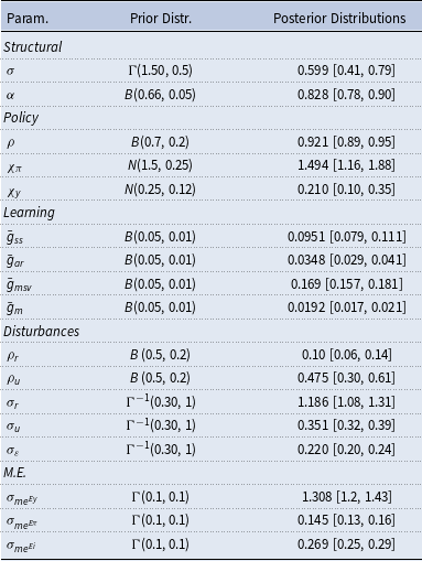
The selected prior distributions are shown in Table 1. I assume a Gamma prior distribution for the intertemporal elasticity of substitution
 $\sigma$
. The Calvo price stickiness parameter follows a Beta prior distribution with mean 0.66 and standard deviation 0.05. The monetary policy reaction coefficients to inflation and output are assumed to follow Normal prior distributions with means 1.5 and 0.25, respectively. The interest-rate smoothing coefficient
 $\rho$
follows a Beta prior with mean 0.7. The autoregressive coefficients for the natural rate and cost-push disturbances similarly follow Beta distributions, which are, however, kept less informative (mean 0.5, standard deviation 0.2). Key parameters in the estimation are the learning gain parameters, which determine how sensitive agents’ beliefs are to new information. I assume Beta (0.05, 0.01) priors for all gain coefficients.Footnote
7
I assume Inverse Gamma priors for the standard deviations of structural innovations and Gamma (0.1, 0.1) priors for the standard deviations of measurement errors. The latter imply probability masses that are higher at zero and progressively declining for larger values: they are meant to penalize higher degrees of measurement error.
4. Results
4.1 Estimates
Table 1 presents the posterior estimates for the structural and learning parameters in the baseline estimation. The estimates for ‘deep’ and policy parameters are in line with previous literature: the posterior mean for
 $\sigma$
is equal to 0.599 and for
 $\alpha$
is equal to 0.828, indicating a large degree of price stickiness. The Taylor rule coefficients have posterior means equal to 0.92 for the inertia
 $\rho$
, 1.49 for the feedback to inflation
 $\chi _{\pi }$
and 0.21 for the reaction to output
 $\chi _{y}$
.
Posterior estimates: baseline estimation

Notes: The Table reports mean posterior estimates, along with 2.5% and 97.5% percentiles.
The presence of expectations data reduces the extent of exogenously needed persistence: the autoregressive parameters for the natural rate and markup disturbances are relatively low at 0.10 and 0.47.Footnote 8
The constant gain coefficient is estimated around 0.095 for the reverting to steady state model, at 0.035 for the backward-looking model, and at 0.169 for the MSV specification. Agents learn about the best forecasting models in similar ways, with a somewhat lower gain coefficient equal to 0.0192.
4.2 Heterogeneous expectations
Figure 2 shows observed inflation expectations from the Survey of Professional Forecasters together with the expectations implied by the three different PLMs. As expected, the first PLM generates expectations that are smoother than actual inflation, as they resemble a moving average of past inflation data. Such expectations reflects the predictions of forecasters who don’t overreact to recent data and shocks but believe that fluctuations are dominated by mean reversion to long-run equilibria. Expectations formed from PLMs 2 and 3 are more volatile, with one responding closely to lagged observations and the other adjusting in response to structural shocks. In particular, MSV expectations would have implied more elevated inflation expectations during the double peaks in the 1970s in response to supply shocks, compared with what observed in the SPF.
Survey inflation expectations and heterogeneous expectations from three PLMs.
Notes: The figure shows observed survey inflation expectations from the SPF and model-implied heterogeneous expectations according to the three Perceived Laws of Motion (PLM): the long-run/steady-state PLM, the AR model PLM, and the PLM based on the MSV solution.

Inflation beliefs.
Notes: The figure shows the evolution of estimated beliefs about: the intercept in the steady-state PLM for inflation; the autoregressive coefficient in the AR-PLM for inflation; the sensitivity of inflation to cost-push shocks in the MSV-PLM.

Output beliefs.
Notes: The figure shows the evolution of estimated beliefs about: the intercept in the steady-state PLM for output; the autoregressive coefficient in the AR-PLM for output; the sensitivity of output to natural-rate demand shocks in the MSV-PLM.

Figures 3 and 4 show the evolution of selected beliefs over the sample. Agents observe higher than expected inflation through the 1970s and, in the mean reversion PLM, progressively revise upward their perceptions about long-run inflation. To a minor extent, they also revise upward their perception in the aftermath of COVID. In the trend-following, AR(1), PLM, they would revise their beliefs about the intercept in the same way, although more slowly. Agents learn that inflation is more persistent than previously assumed in the early 1970s. Positive forecast errors in that period lead to revisions in both coefficients in the same direction. Agents then maintain stable beliefs until around 2010 when they revise downward their estimates of intrinsic inflation inertia. Perceived inflation persistence remains low for a decade, before quickly dropping, and then substantially rising up again post-COVID. In the MSV PLM, beliefs about the sensitivity of inflation to markup shocks
 $u_{t}$
assume a special importance. The perceived impact of such shocks on inflation also increases during the COVID episode.
Turning to output beliefs, perceptions about its persistence move generally less than for inflation: agents realize that its autoregressive coefficients is close to 1 everywhere in the sample. The exception is given by the COVID years. The perceived inertia spikes up above one, before falling during the unexpectedly rapid recovery. Expectations in the MSV model also become additionally sensitive to exogenous shocks in the same years.
Model weights for inflation expectations.
Notes: The figure shows the evolution of estimated model weights corresponding to the steady-state, AR, and MSV perceived models.

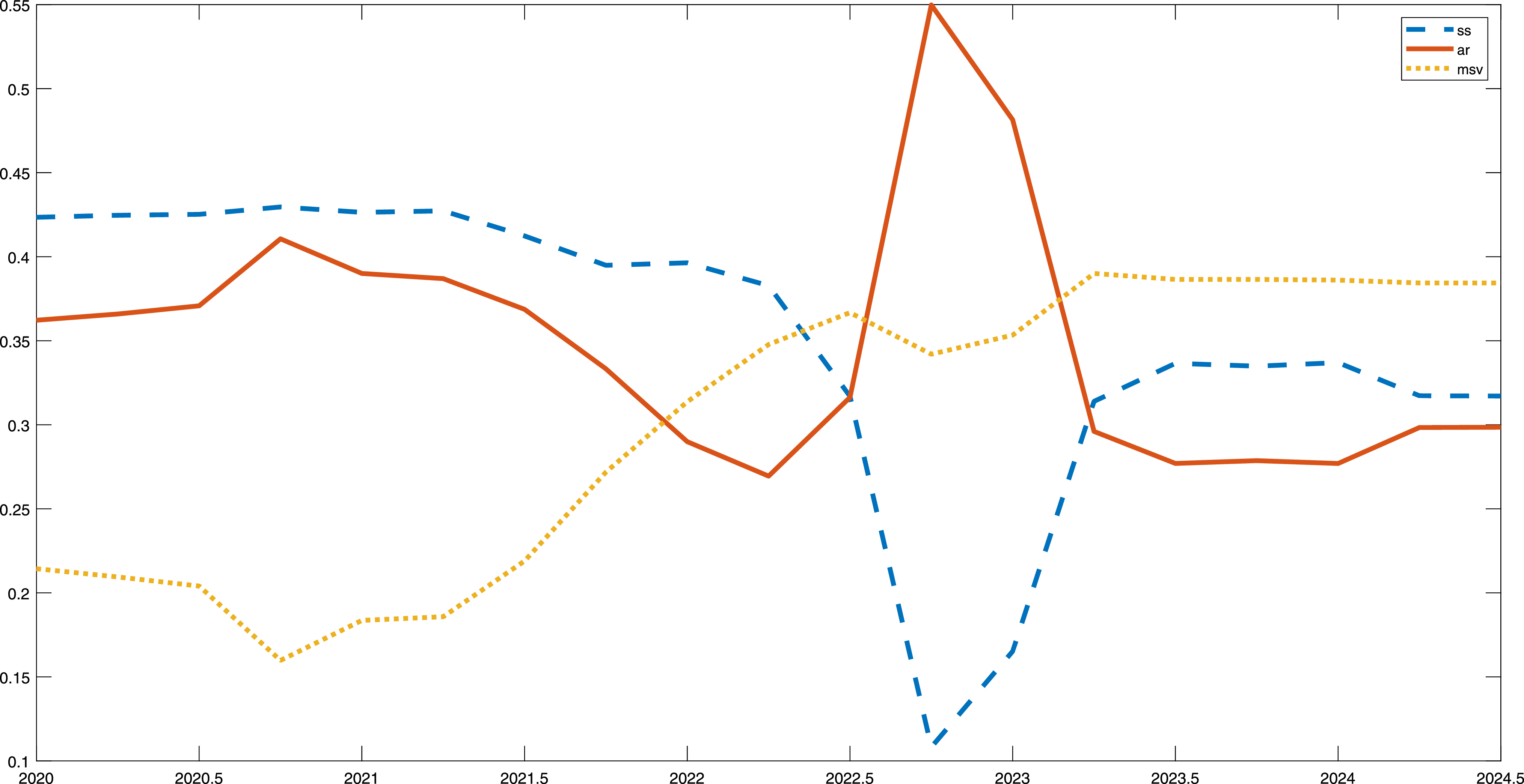
Besides learning about coefficients within each single model, agents also learn about the reliability of different models. They revise their model weights over time through a similar constant-gain learning algorithm. Figure 5 illustrates the shifts in model weights. Both the mean-reversion and AR PLMs increase in importance in the 1970s, together with rising perceptions about the mean and autocorrelation of inflation. Figure 6 presents a zoomed-in view of the later years to highlight the remarkable shift in beliefs in correspondence of the COVID pandemic. Agents progressively discard the mean reversion world view (with about a 10% share in late 2022) in favor of increased reliance on the trend-following model, which captures a share around 55%. This shift suggests a non-trivial amount of unanchoring of expectations, with inflation believed to be more persistent than in the past.
Model weights for inflation expectations: COVID sample.
Notes: The figure shows the evolution of estimated model weights corresponding to the steady-state, AR, and MSV perceived models, during the COVID years (2020–2024).

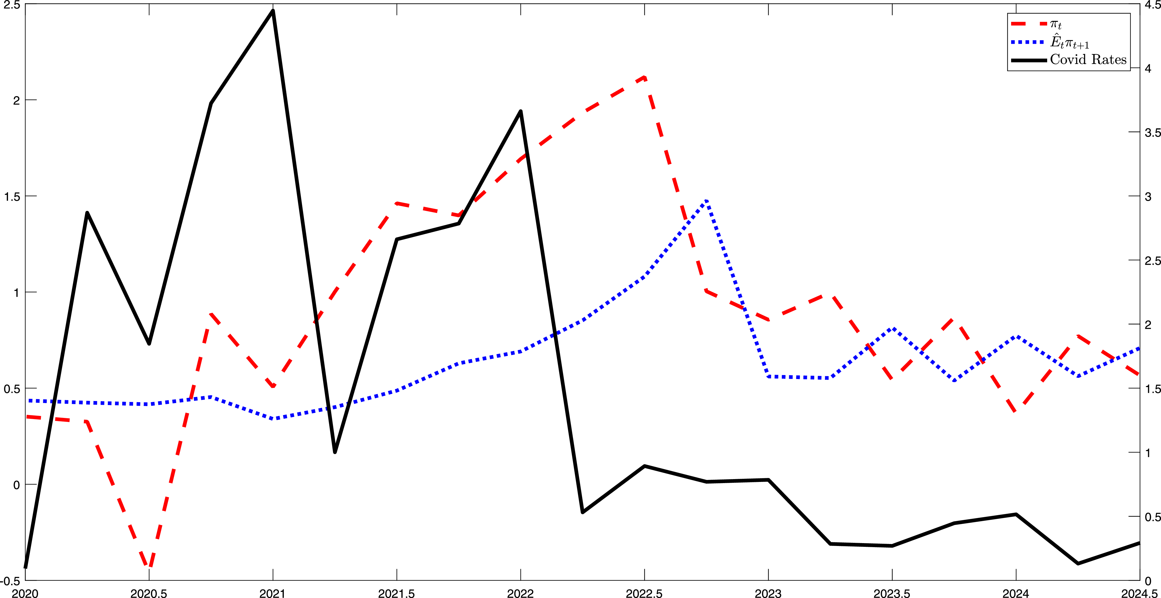
Evolution of realized inflation, aggregate inflation expectations, and COVID rates, over the COVID sample.
Notes: The figure compares the evolution of realized inflation, model-implied aggregate inflation expectations, and COVID death rates per 100,000 population. The labels in the left Y-axis refer to inflation and inflation expectations; those in the right Y-axis refer to COVID rates.

Figure 7 clarifies the story behind the evolution of aggregate expectations.Footnote 9 The figure shows the COVID death rates per 100,000 population (provided by the CDC) in the U.S. as a measure of the severity of the pandemic over those years. In the early pandemic quarters, inflation falls below target because of the COVID-induced recession. Expectations, however, remain roughly stable. During 2021 and the first half of 2022, inflation rates constantly rise. As a result, expectations also begin to move and they progressively increase for almost two years. This is the period in which agents revised their perceptions and model views, as documented earlier. Expectations continue to rise even after inflation has started to fall. Expectations begin to revert back later on, although they remain above their historical average. The behavior of expectations in the first part of the pandemic is consistent with the survey evidence; for example, as discussed in Reis (Reference Reis2023), mean expectations initially don’t react. The first signs of instability in inflation expectations manifest itself instead in their dispersion, which increases before the mean starts moving.
4.2.1 Dispersion
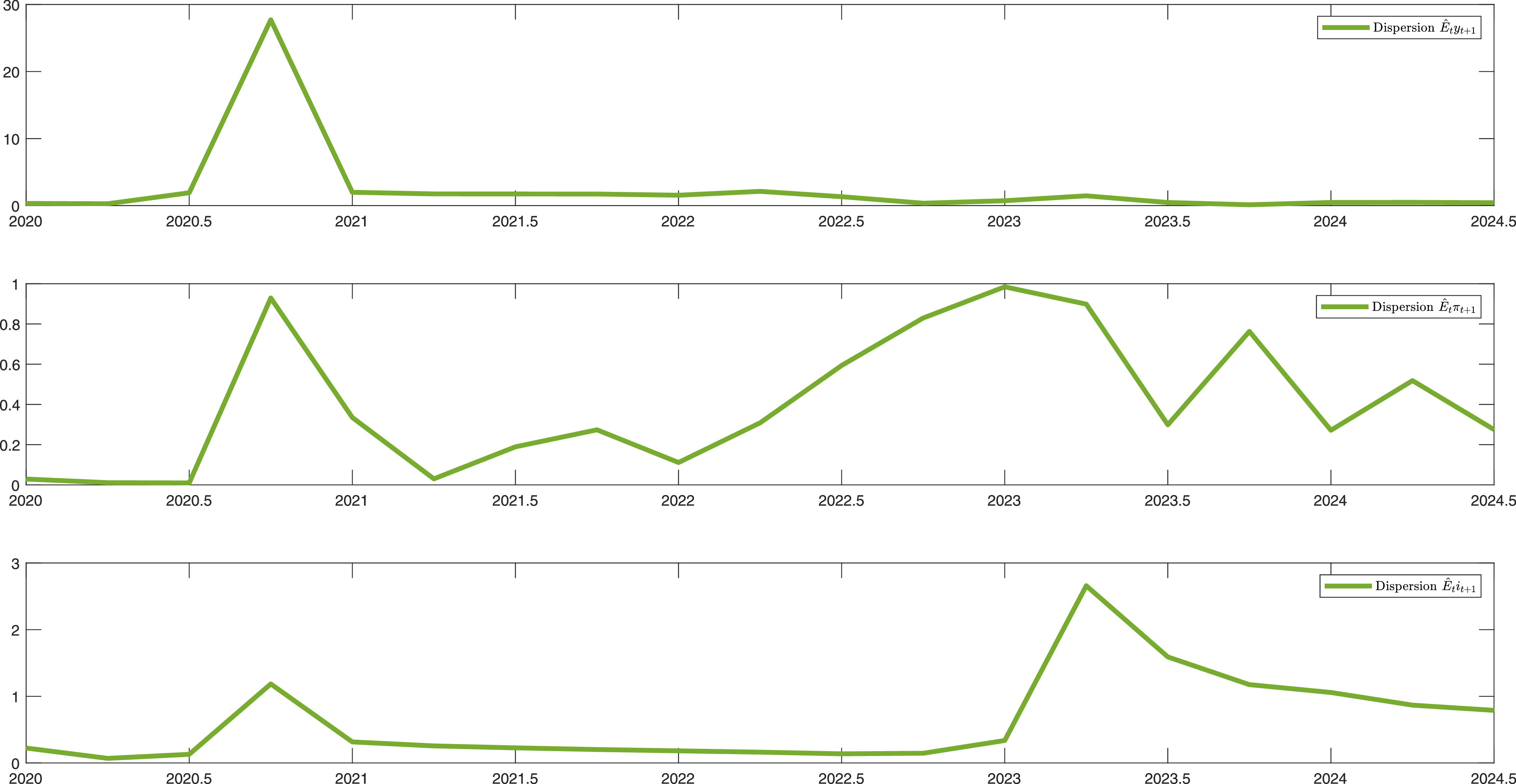
Figure 8 shows how the dispersion of heterogeneous expectations in the model changes in response to the COVID pandemic. Dispersion related to output expectations significantly increases in response to the COVID shock between the second and third quarters of 2020; it is lower later on after the relatively rapid recovery in real activity. The dispersion of inflation expectations rises in the same period at the beginning of the pandemic, but it also rises, and more persistently so, in its aftermath, when observed inflation rates increase in 2022 and 2023. Finally, uncertainty about the monetary policy response to rising inflation increases the dispersion of interest rate expectations in 2023 and afterwards. Disagreement about expected policy was instead lower in response to the COVID shock, since economic agents anticipated that monetary policy would turn expansionary.
Dispersion of heterogeneous output, inflation, and interest rate expectations (COVID sample).
Notes: The figure shows the evolution of model-implied disagreement across heterogeneous expectations about output, inflation, and interest rates, over the COVID years.

4.3 Inflationary shocks and monetary policy
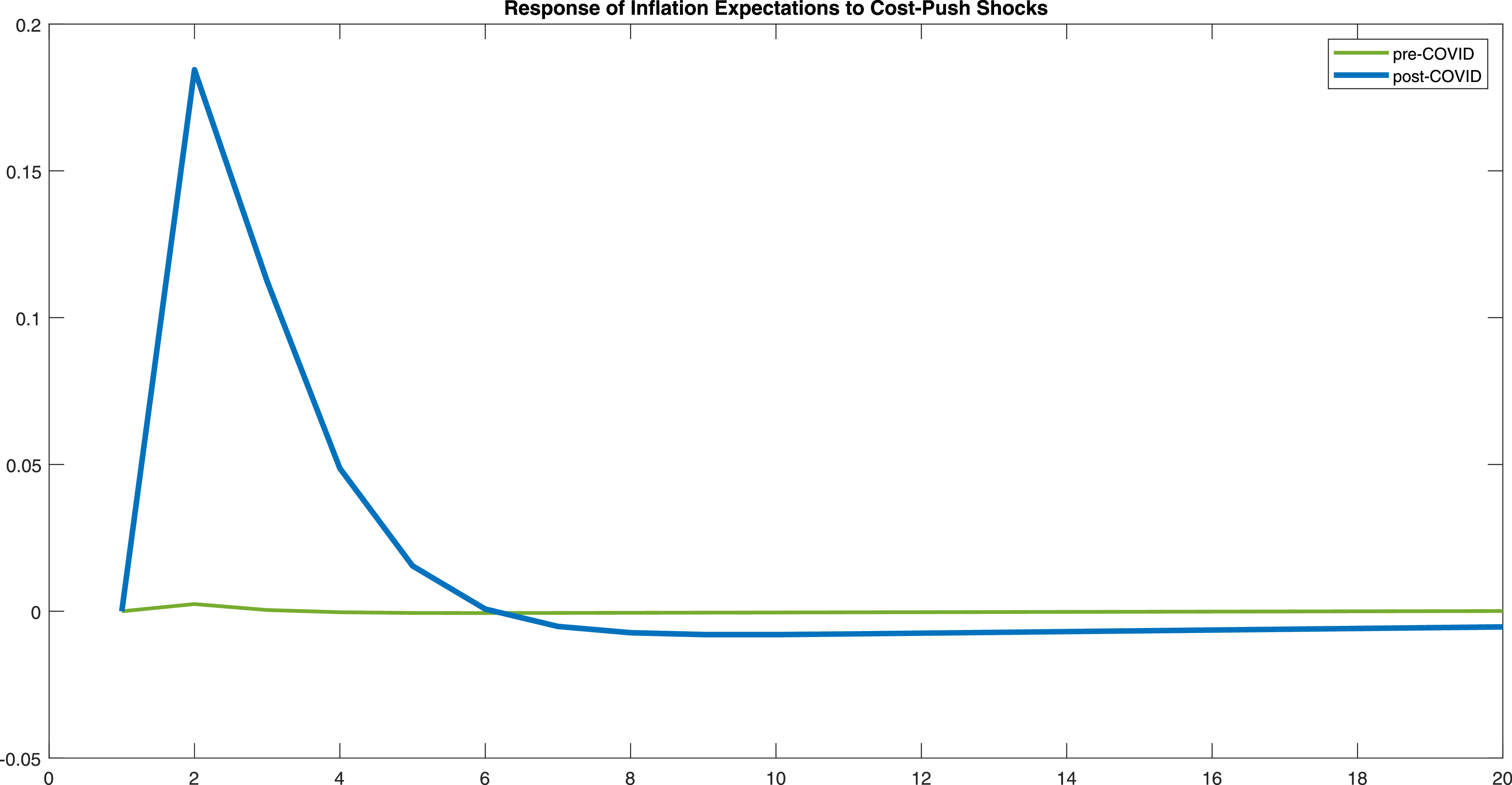
The impact of inflationary markup shocks may be severely affected by the prevailing state of expectations. Figure 9 compares the response of inflation expectations to cost-push shocks just before the pandemic (first quarter of 2020) and in its aftermath (third quarter of 2022). In only a few quarters, it’s evident that expectations have partially unanchored. In 2022, the share of forecasters who use the mean reversion PLM is at its historical low around 0.1 and the share of trend-following forecasters spikes. As a result, the impulse response of inflation expectations to the inflationary shock becomes much stronger. The response was almost imperceptible before COVID, due to different prevailing models that were more consistent with anchored expectations.
Impulse response function of inflation expectations to cost-push shocks.
Notes: The figure compares responses before COVID (2020:I, green line) and after COVID (2022:III, blue line). For the computation of impulse responses, the model parameters are set at their estimated posterior mode values.

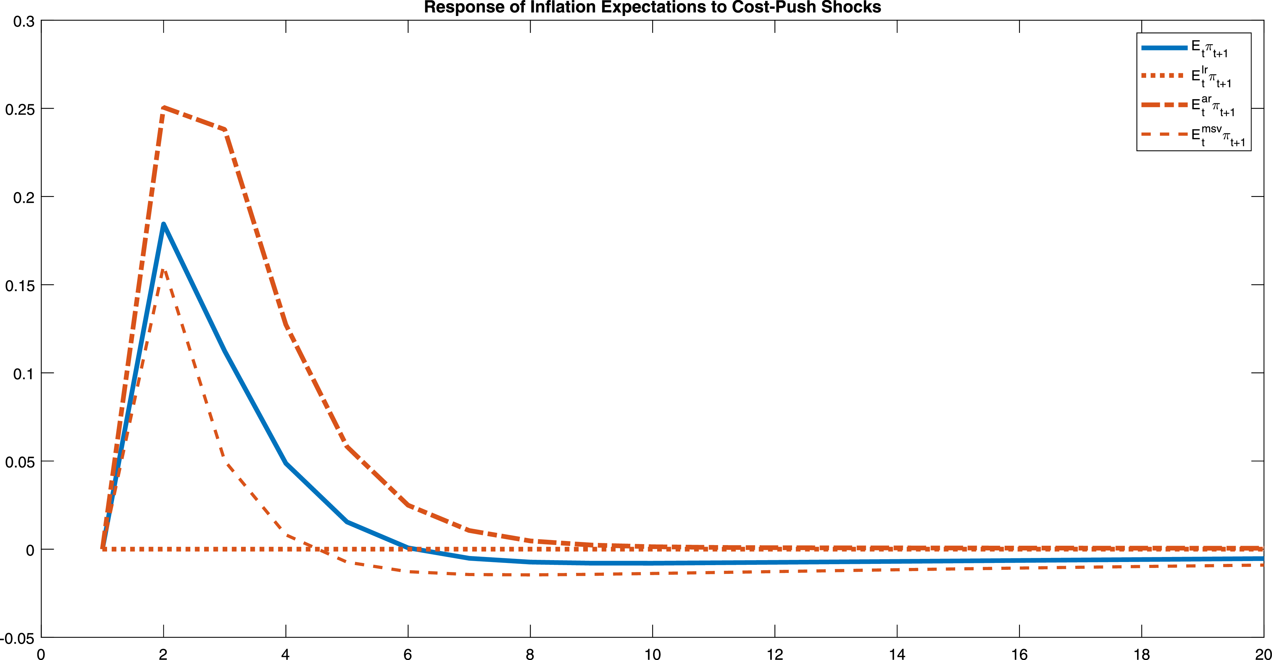
Impulse response function of heterogeneous inflation expectations to cost-push shocks.
Notes: The figure compares the impulse responses of aggregate and heterogeneous expectations to supply shocks; heterogeneous expectations refer to those obtained from the long-run/steady-state, autoregressive, and MSV models.

Figure 10 shows the behavior of heterogeneous expectations under alternative perceived models. The long-run and MSV models lead to more muted responses than those observed in the data. The AR, trend-following, model induces more persistence into the economy, and it leads to stronger responses of expectations. The larger the share of this type of expectations, the larger the sensitivity of aggregate expectations to temporary shocks.
4.4 Monetary policy and shifting expectations
The effects of monetary policy can similarly depend on the prevailing perceptions about the economy.
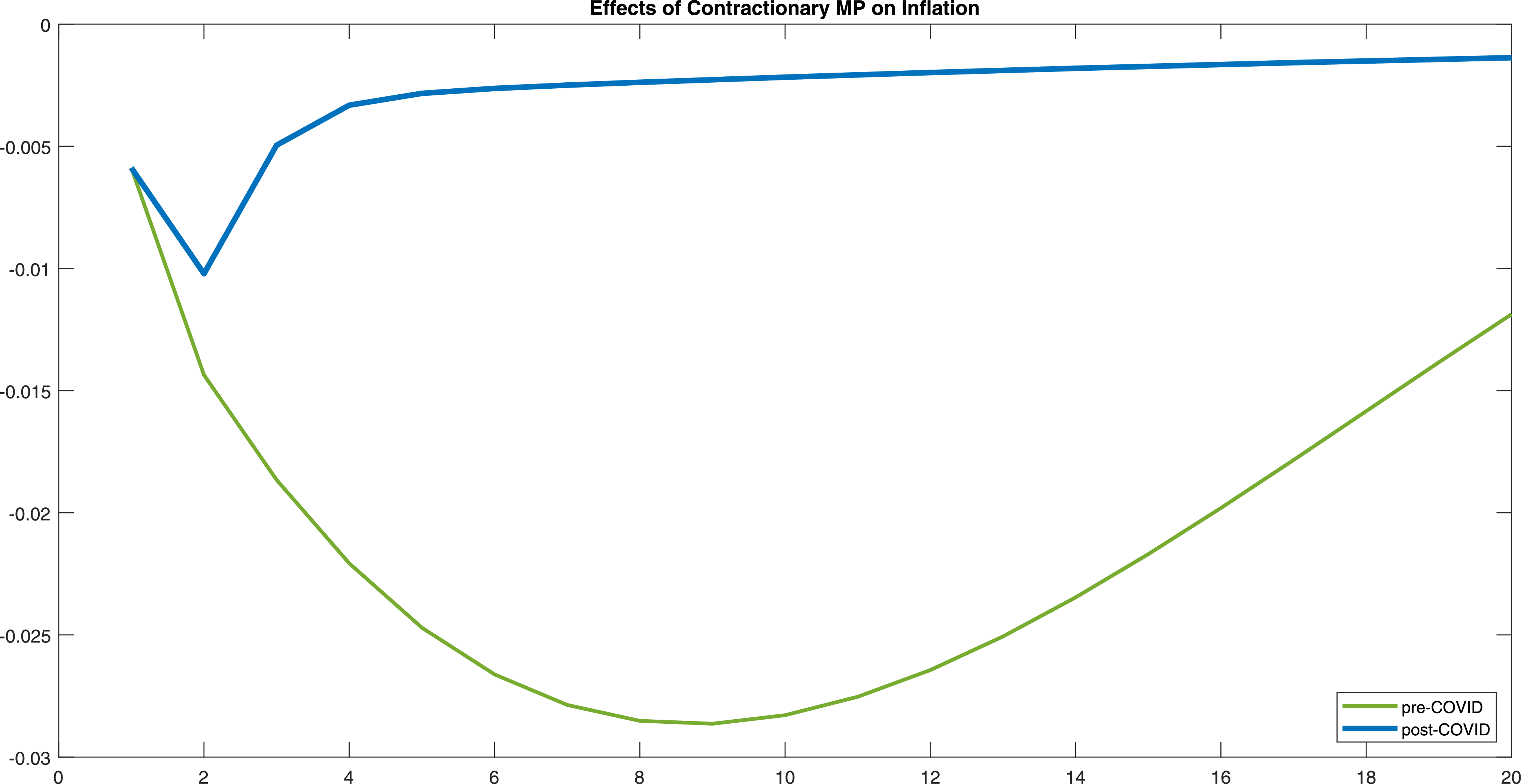
As shown in Figure 11, the effectiveness of contractionary monetary policy in reducing inflation diminishes between 2020 and 2022, with the unanchoring of expectations due to the larger share of trend-following forecasters. These findings, therefore, suggest that monetary policy need to become more aggressive toward inflation when expectations become less anchored, in this case due to a shift away from perceived models consistent with mean reversion into models based on trend-following.
Impulse response function of inflation to contractionary monetary policy shocks.
Notes: The figure compares responses before COVID (2020:I, green line) and after COVID (2022:III, blue line). For the computation of impulse responses, the model parameters are set at their estimated posterior mode values.

5. Robustness
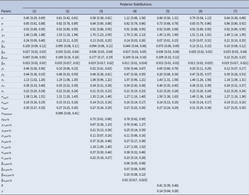
I assess the sensitivity of the results under alternative specifications and modeling choices. Table 2 reports the corresponding posterior estimates for each specification.
Posterior estimates: alternative specifications for robustness

Notes: The Table reports mean posterior estimates, along with 2.5% and 97.5% percentiles. The estimates under each column correspond to the following specification: (1) Model with no restrictions on weights; (2) Model with anticipated monetary policy news shocks during ZLB periods; (3) Model with time variation in monetary policy and shock coefficients; (4) Model with time variation in monetary policy, shock, and constant gain coefficients; (5) Extended model with habit formation in consumption and price indexation to past inflation; (6) Model with two forecasting PLMs; (7) Model with endogenous switching gains.
5.1 No restrictions on model weights
The baseline estimation restricted the model weights to sum to one (
 $\omega _{t}^{ss}+\omega _{t}^{ar}+\omega _{t}^{msv}=1$
at each
 $t$
). I re-estimate the model without imposing this assumption. In terms of the coefficients, the main changes are that the constant gain for the MSV perceived model is estimated at a lower value at 0.047. The natural rate disturbance is more persistent in this estimation.
5.2 Zero-lower bound periods
Two periods in our sample are characterized by a binding zero-lower-bound constraint: the post-Financial Crisis years between 2009 and 2015 and the COVID quarters between 2020 and early 2022. The baseline estimation ignores the ZLB under the assumption that the resulting bias on the posterior estimates remains small enough (in this case, the deviations from the typical Taylor rule in the ZLB periods would simply be captured by the exogenous component
 $\varepsilon _{t}$
). Here, I deal with the ZLB in a different way: when the policy rate is cut to zero, I introduce a news shock component in the Taylor rule, as in Del Negro et al. (Reference Del Negro, Giannoni and Patterson2023).Footnote
10
The Taylor rule becomes:
 \begin{align} i_{t} &= \rho i_{t-1}+(1-\rho )\left [\chi _{\pi }\pi _{t}+\chi _{y}y_{t}\right ]+\varepsilon _{t}+\eta _{t-k}^{k}, \end{align}
where
 $\eta _{t-k}^{k}$
denotes a policy news shock, which is anticipated
 $k$
periods ahead (here, for simplicity, I assume
 $k=1$
). The prior for the standard deviation of the news shock is
 $\Gamma (0,1,0.1)$
. The estimates in Table 2 show that the introduction of a news shock to deal with the ZLB doesn’t substantially affect the posterior estimates.
5.3 Shifts in monetary policy & macro volatility
The model has been estimated by assuming constant parameters (except for learning beliefs and shifting model weights) for the whole sample. Many papers, however, document shifts in monetary policy coefficients and in the standard deviation of the shocks before and after the appointment of Volcker as Fed’s Chairman in 1979 (e.g., Lubik and Schorfheide, Reference Lubik and Schorfheide2004). I account for possible time variation by allowing the monetary policy parameters
 $\rho$
,
 $\chi _{\pi }$
,
 $\chi _{y}$
, and the standard deviations of the shocks
 $\sigma _{\varepsilon }$
,
 $\sigma _{r}$
,
 $\sigma _{u}$
, to shift values before and after 1979.
As a second, related, case, I also re-estimate the model with the same time-varying parameters but also allowing the constant gain coefficients to change values in the pre- and post-1979 samples (Milani, Reference Milani2014, for example, finds higher gain coefficients in the earlier sample). The estimates support the evidence of a structural break in the monetary policy coefficients: the response to inflation increases from below 1 before Volcker to 1.7 after Volcker.Footnote
11
Policy also becomes more gradual (with
 $\rho$
increasing from 0.75 to 0.92) and less responsive to real activity (with
 $\chi _{y}$
declining from 0.21 to 0.13). The shocks become less volatile in the second sample. The evidence for time variation in constant gains is more mixed.
5.4 Extended model with endogenous sources of inertia
It is typical in rational expectation DSGE models to introduce additional sources of inertia to fit macroeconomic data. The most common choices are the assumption of habit formation in consumption and indexation to lagged inflation in price setting. These two extensions provide a microfoundation for lagged terms in the output Euler equation and in the New Keynesian Phillips curve. I re-estimate the extended model that includes habits and indexation, denoted by coefficients
 $h$
and
 $\gamma$
, both assumed to follow Beta (0.5, 0.2) prior distributions. The data support a medium level of habit formation (
 $h=0.41$
), while they indicate only minimal indexation (
 $\gamma =0.14$
).
5.5 Only two forecasting models
As an additional sensitivity test, I estimate a simpler specification, which allows for two shifting models instead of three. I retain the steady state and the trend-following forecasting models, and remove the MSV case. Overall, there are no significant changes in the estimates.
5.6 Endogenous time-varying gains
The main estimation assumes learning with constant gains for the parameters in each perceived model and for learning about the model themselves. An alternative in the literature is the use of recursive least squares (RLS) learning, which assumes a decreasing gain equal to
 $t^{-1}$
in each period. RLS learning is used in theoretical work to test the convergence of beliefs to the rational expectations equilibrium; it is typically abandoned in favor of constant-gain learning in empirical work, since the latter allows agents to remain more reactive to new observations even with longer samples. A decreasing gain would imply beliefs that stabilize as
 $t$
increases and become unresponsive to any potential structural change.
While a decreasing gain over the full sample is likely unrealistic, here I still decide to assess the sensitivity of the result to alternative gain assumptions by using the endogenous, time-varying gain used in Marcet and Nicolini (Reference Marcet and Nicolini2003) and Milani (Reference Milani2014). These gains incorporate the benefits of both decreasing and constant gains: when forecast errors are large by historical standards, agents worry about structural breaks and switch to a constant gain, which gives more weight to new information and discount older observations. When forecast errors are below their historical averages, on the other hand, agents retain confidence in the accuracy of their model and adopt a decreasing gain, which is relatively unresponsive to new data. The resulting gain can, therefore, switch endogenously between
 $\bar {g}$
and
 $t^{-1}$
, depending on the values of recent forecast errors, and becomes time-varying.
I re-estimate the model with the time-varying gains. I still estimate the value for the same constant gain coefficients
 $\bar {g}_{ss}$
,
 $\bar {g}_{ar}$
,
 $\bar {g}_{\textit{msv}}$
, and
 $\bar {g}_{m}$
, but now they refer only to those instances in which the time-varying gain switches to constant. The posterior estimates for the gains remain overall similar, with a slightly higher mean for
 $\bar {g}_{\textit{msv}}$
.
—–
As shown, in terms of posterior estimates, the values remain comparable across all the alternative specifications. There is some more pronounced variation in the value of
 $\sigma$
, the elasticity of intertemporal substitution, which mirrors the wide range of estimates typically found in the literature.
Robustness. Model weights for inflation expectations and belief about inflation persistence across estimated specifications (COVID sample).
Notes: In the top panel, the Figure superimposes the estimated model weights for the steady-state (blue dashed lines) and AR (red solid lines) PLMs, across all the robustness specifications estimated in Section 5. In the bottom panel, it superimposes the evolution of estimated beliefs about the persistence of inflation, across the same specifications.

Besides looking at the estimates, to evaluate the robustness of the main results, I compare the evolution of the model weights assigned to the steady-state and to the autoregressive PLMs during the COVID sample and across the previous estimated specifications. I also compare the perceived inflation persistence by agents during the same period. Figure 12 shows the resulting, superimposed series. In all robustness cases, agents revise their beliefs to assign more weight to the trend-following model and less to the mean reversion model in the second half of 2022. Similarly, consistently across all specifications, agents initially revise downward their perceptions of inflation persistence (in late 2020/early 2021) and then they strongly revise the perceived persistence upward in 2021 and 2022. Overall, the main story during the COVID years seems robust to the different modeling choices.
6. Conclusions
After decades of price stability and anchored expectations, high inflation has made a comeback in the aftermath of the COVID pandemic.
This paper has revisited the history of U.S. inflation, real activity, and monetary policies through the lens of a macroeconomic model that assigns a central role to shifting heterogeneous expectations. The expectation formation models capture different behavioral features: for some agents, it could be a belief that the economy rapidly returns to its long-run equilibrium after shocks; for others, trend-following behavior, which can create intrinsic persistence through sluggish expectations; finally, other agents may have smaller deviations from rational expectations but still engage in learning based on recent experiences.
The results show that shifts in heterogeneous expectations played a role in the unexpected return of high inflation after COVID. Agents discarded beliefs that assumed inflation as quickly reverting to target and began to form expectations more adaptively. They rapidly revised upward their perceptions of how persistent deviations of inflation from target could be.
Due to the shift in beliefs, inflation expectations became less anchored and, thus, more reactive to transitory shocks than they were a few quarters before. The partial unanchoring of expectations, in turn, reduces the effectiveness of contractionary monetary policy to bring inflation under control.
In the paper, I concentrated the discussion on inflation after COVID. But a similar mechanism plays a role during different episodes, characterized by abrupt shifts in inflation behavior, such as the run-up of inflation in the 1970s and the change in monetary policy regime leading to Volcker’s disinflation. Shifts in heterogeneous expectations may be even more relevant in other economies, particularly those with long traditions of high inflation.
Furthermore, the model doesn’t simply explain high-inflation episodes. It can similarly help account for the dynamics of inflation in normal times. In those cases, the model shares will likely be different and dominated by the mean-reversion belief. However, this framework emphasizes that, even in normal times, stability may be fragile: a sequence of observations in the same direction may lead to shifts in agents’ perceived models and potentially pose dangers for the control of inflation.
Acknowledgements
I would like to thank organizers and participants at the 4th Workshop on Financial Econometrics and Empirical Modeling of Financial Markets: New Challenges for Monetary Policy and Financial Markets at the Technical University of Freiberg, and particularly the paper’s discussant Dominik Hecker, for insightful comments and discussions. I’m also grateful to organizers and participants at the Bank of Canada’s Next Generation Modelling Workshop and to my discussant Tao Wang, for helpful feedback and conversations. Addresses for Correspondence: Department of Economics, 3151 Social Science Plaza, University of California, Irvine, CA 92697-5100, U.S.A. Email: fmilani@uci.edu. Homepage: https://sites.socsci.uci.edu/∼fmilani.