1 Introduction
Viscous gravity currents result from density-driven flows in highly viscous materials, which have been the subject of many theoretical and experimental investigations. Various geometries have been considered, including simple single-layer flow over a rigid horizontal boundary (Smith Reference Smith1969; Huppert Reference Huppert1982a ; Gratton & Minotti Reference Gratton and Minotti1990), two-layer flows at a horizontal boundary or interface (Hoult Reference Hoult1972; Lister & Kerr Reference Lister and Kerr1989; Koch & Koch Reference Koch and Koch1995; Kowal & Worster Reference Kowal and Worster2015), flows down slopes (Smith Reference Smith1973; Huppert Reference Huppert1982b ; Lister Reference Lister1992), non-Newtonian currents (Nye Reference Nye1952; Griffiths & Fink Reference Griffiths and Fink1993; Fink & Griffiths Reference Fink and Griffiths1998; Gratton & Minotti Reference Gratton and Minotti1999; Balmforth et al. Reference Balmforth, Craster, Perona, Rust and Sassi2007; Hogg & Matson Reference Hogg and Matson2009; Sayag & Worster Reference Sayag and Worster2013), currents with leakage (Acton, Huppert & Worster Reference Acton, Huppert and Worster2001; Pritchard & Hogg Reference Pritchard and Hogg2002; Neufeld et al. Reference Neufeld, Vella, Huppert and Lister2011), flow underneath an elastic sheet (Lister, Peng & Neufeld Reference Lister, Peng and Neufeld2013; Hewitt, Balmforth & De Bruyn Reference Hewitt, Balmforth and De Bruyn2015) and flow towards a central hole (Diez, Gratton & Gratton Reference Diez, Gratton and Gratton1992; Zheng, Christov & Stone Reference Zheng, Christov and Stone2014). These phenomena are of wide interest in many contexts, for example, in industrial applications and geological systems (Huppert Reference Huppert2006), such as lava flows (Griffiths Reference Griffiths2000) and ice sheets (Schoof & Hewitt Reference Schoof and Hewitt2013).
Theoretical analysis of the propagation of viscous gravity currents often makes use of lubrication theory, which is valid in the case of currents that are long and thin. Under these assumptions, many similarity solutions can be found, which describe the self-similar spreading of the fluids involved in many different geometries (see e.g. Gratton & Minotti Reference Gratton and Minotti1990). Beyond enabling prediction of the shapes and spreading rates of the currents, these base-state similarity solutions can also be used to perform linear stability analyses of possible symmetry-breaking instabilities. Examples include the linear stability of a single-layer current over a horizontal surface in a porous medium (Mathunjwa & Hogg Reference Mathunjwa and Hogg2006) and the fingering instability that occurs when a fluid flows down a slope (Huppert Reference Huppert1982a ).
Two-layer gravity currents with a free surface and with a non-zero density difference between the injected and ambient fluids were studied by Lister & Kerr (Reference Lister and Kerr1989), motivated by application to the viscous spreading of the lithosphere along the mid-mantle boundary (Kerr & Lister Reference Kerr and Lister1987). The authors identified different regimes for deep and shallow ambient layers compared to the radius of the spreading current. They considered the self-similar spreading of currents with influx rates proportional to
 $t^{\unicode[STIX]{x1D6FC}}$
, for both axisymmetric flows and two-dimensional (2-D) flows. For spreading over a shallow ambient layer, they found critical values
 $\unicode[STIX]{x1D6FC}=1$
(constant influx) for axisymmetric spreading and
 $\unicode[STIX]{x1D6FC}=1/2$
for two dimensions; for smaller
 $\unicode[STIX]{x1D6FC}$
the current thins and remains shallower than the ambient, while for larger
 $\unicode[STIX]{x1D6FC}$
the current thickens and approaches the behaviour of a single-layer gravity current as in Huppert (Reference Huppert1982a
). The equations for the critical case, where the upper- and lower-layer thicknesses remain comparable (i.e.
 $\unicode[STIX]{x1D6FC}=1$
for axisymmetric spreading,
 $\unicode[STIX]{x1D6FC}=1/2$
for two dimensions), were derived in an appendix and some numerical solutions were presented for the 2-D case. Lister & Kerr (Reference Lister and Kerr1989) also conducted experiments in the deep and shallow regimes, measuring the extent of the current as a function of time and finding good agreement with the predicted scaling for the self-similar nose position. However, the actual profiles of the currents were not compared and, for the critical case of constant influx in the axisymmetric geometry, their model only applies at small influxes, where the spreading current is much thinner than the ambient layer.
In this paper we look at the critical case of an axisymmetric two-layer current with a fixed influx of one fluid into and over a pre-existing lubricating layer of a second fluid. In particular, we focus on the limit of equal densities, which we find is singular. The theoretical solutions are also compared with experimentally measured profiles.
Another type of a two-layer gravity current was studied by Kowal & Worster (Reference Kowal and Worster2015) who analysed concurrent spreading of two injected fluids over a horizontal rigid surface with the upper, lighter fluid extending further due to being lubricated by the lower, less viscous fluid. While the authors also found shocks in the equal-density limit, the mechanism is quite different from that described in this paper, and derives from their implementation of the rigid lower boundary condition.
The mathematical analysis of the limit of equal densities in our problem bears some resemblance to that for intrusion of a fluid into a Hele-Shaw cell filled with a fluid of equal density but different viscosity. A key distinction in the Hele-Shaw problem is the question of whether surface tension is significant or can be ignored. For miscible fluids or those with negligible surface tension, Wooding (Reference Wooding1969) found and described a fingering instability comparable to the well-known Saffman–Taylor instability for flows with surface tension (Saffman & Taylor Reference Saffman and Taylor1958; Saffman Reference Saffman1986). Further work by Paterson (Reference Paterson1985) carried out a linear stability analysis for the limit of an inviscid intruding fluid with no surface tension in a Hele-Shaw cell, which predicted instability for all parameters and a most unstable wavelength that compared well to his experimental results. Yang & Yortsos (Reference Yang and Yortsos1997) extended this analysis to viscous intruding fluids, resolving the cross-sectional structure of the intruding flow using lubrication theory. They derived a kinematic evolution equation for the interfacial position, which we show bears some resemblance to the evolution equation of the interface in a two-layer gravity current. They found that, for sufficiently less viscous intrusions, vertical discontinuities, called shocks, are predicted by the kinematic equation to develop at the nose. The exact nature of these frontal shocks remains unclear as the shock height predicted by Yang & Yortsos (Reference Yang and Yortsos1997) disagreed with experimental measurements by Petitjeans & Maxworthy (Reference Petitjeans and Maxworthy1996) and with numerical simulations by Chen & Meiburg (Reference Chen and Meiburg1996) and Rakotomalala, Salin & Watzky (Reference Rakotomalala, Salin and Watzky1996). Yang & Yortsos (Reference Yang and Yortsos1997) proposed that the shocks at the nose can plausibly be regularised by a local, fully two-dimensional Stokes flow around the nose, where lubrication theory breaks down, and that this would change the shock-fitting condition. To our knowledge, there has not been any work done confirming this conjecture. More recently, other work has extended the basic ideas of Yang & Yortsos (Reference Yang and Yortsos1997). For example, Lajeunesse et al. (Reference Lajeunesse, Martin, Rakotomalala and Salin1997, Reference Lajeunesse, Martin, Rakotomalala, Salin and Yortsos1999, Reference Lajeunesse, Martin, Rakotomalala, Salin and Yortsos2001) analysed the flow in a vertical Hele-Shaw cell, including stabilising density differences in the analysis, and experimentally measured a critical viscosity ratio for the onset of a fingering instability. These authors also suggested a link between the instability and the formation of shocks by adapting the arguments of Saffman & Taylor (Reference Saffman and Taylor1958) to the vicinity of a shock. Bischofberger, Ramachandran & Nagel (Reference Bischofberger, Ramachandran and Nagel2014) found a different critical viscosity ratio for the onset of instability experimentally, but also suggested that the pressure drop associated with the steep interface is the key instability mechanism.
There are two significant differences between flows in a Hele-Shaw cell and the two-layer gravity currents analysed in this paper. Firstly, the free top surface of a two-layer gravity current is evolving and hence the total thickness of the current varies in space and time. Secondly, the pressure gradients caused by non-zero but small density differences in a two-layer gravity current allow an explicit regularisation of any vertical shock discontinuities that may form.
The objective of this paper is to develop the theory for the self-similar spreading of one fluid over a second fluid of differing viscosity but equal, or nearly equal, density. Surface tension and diffusion are assumed to be negligible.
The mathematical model for this spreading includes the evolution of the top surface, which adds complexity over the simpler model for a Hele-Shaw cell with fixed total height. However, we find that by including the regularising effect of small non-zero density differences, we obtain physically justified, so-called ‘entropy’ conditions for the evolution of any shock that develops. Therefore, modelling two-layer gravity currents provides a much better starting point for future linear stability analyses as the nature of the nose can be understood more easily with an exact condition for the frontal shock height in an axisymmetric similarity solution.
The set-up of the model and its assumptions are described in § 2. The case of equal densities discussed in § 3 is a singular limit of the model discussed in Lister & Kerr (Reference Lister and Kerr1989) and it extends the Hele-Shaw model in Yang & Yortsos (Reference Yang and Yortsos1997) to include a free surface. The regularising mechanism given by small density differences is used to derive closed-form, consistent shock conditions. An illustrative calculation of a simplified time-dependent system in § 4 is used to motivate the physically appropriate boundary conditions for a similarity solution. This leads to a closed system of ordinary differential equations, which is solved numerically in § 5. In § 6 these solutions are compared to the results of laboratory experiments in which we measured the extent and the top surface profiles of currents for various fluid properties and fluxes.
2 Model description
We consider a two-layer axisymmetric gravity current spreading over a rigid horizontal surface. The upper fluid is introduced at a constant volumetric rate
 $Q$
at the origin and spreads radially over a lower layer of fluid, which initially covers the entire horizontal plane with a constant thickness
 $h_{\infty }$
, as shown in figure 1. The fluids have viscosities
 $\unicode[STIX]{x1D707}_{i}$
and densities
 $\unicode[STIX]{x1D70C}_{i}$
, where
 $i=1$
corresponds to the upper, intruding fluid and
 $i=2$
to the lower, lubricating fluid. We define the horizontal extent of the current
 $r_{\ast }(t)$
, the total height
 $h(r,t)$
and the upper-layer thickness
 $d(r,t)$
. Surface tension and diffusion are assumed to be negligible.
Schematic illustration of the set-up and the definition of variables. The fluid properties give rise to a viscosity ratio
 $m=\unicode[STIX]{x1D707}_{2}/\unicode[STIX]{x1D707}_{1}$
and a relative density difference
 $\unicode[STIX]{x1D700}=\unicode[STIX]{x1D70C}_{2}/\unicode[STIX]{x1D70C}_{1}-1$
.

After a short initial transient, the horizontal extent of the current is significantly greater than the vertical extent,
 $r_{\ast }\gg h$
. In this limit, the vertical velocity is negligible and the pressure
 $p$
is therefore hydrostatic to leading order. Using these simplifying assumptions and taking a constant pressure at the free surface we may write
 $$\begin{eqnarray}p=\left\{\begin{array}{@{}ll@{}}\unicode[STIX]{x1D70C}_{1}g(h-z), & h-d<z<h,\\ \unicode[STIX]{x1D70C}_{1}g(h-z)+(\unicode[STIX]{x1D70C}_{2}-\unicode[STIX]{x1D70C}_{1})g(h-d-z), & 0<z<h-d,\end{array}\right.\end{eqnarray}$$
where
 $z$
the height above the bottom surface,
 $g$
the acceleration due to gravity and
 $h(r,t)$
is the position of the free surface.
The pressure gradient then drives a flow, whose horizontal velocity
 $u(r,z,t)$
is given by
 $$\begin{eqnarray}\unicode[STIX]{x1D707}\frac{\unicode[STIX]{x2202}^{2}u}{\unicode[STIX]{x2202}z^{2}}=\frac{\unicode[STIX]{x2202}p}{\unicode[STIX]{x2202}r},\end{eqnarray}$$
with boundary conditions
 $$\begin{eqnarray}\displaystyle \left.\begin{array}{@{}c@{}}\displaystyle u=0\quad \text{at }z=0,\quad \frac{\unicode[STIX]{x2202}u}{\unicode[STIX]{x2202}z}=0\quad \text{at }z=h,\\ \displaystyle [u]_{-}^{+}=0\quad \text{at }z=h-d,\quad \left[\unicode[STIX]{x1D707}\frac{\unicode[STIX]{x2202}u}{\unicode[STIX]{x2202}z}\right]_{-}^{+}=0\quad \text{at }z=h-d.\end{array}\right\} & & \displaystyle\end{eqnarray}$$
The boundary conditions impose no slip at the bottom, no stress at the top surface and velocity and stress continuity at the interface between the fluids, respectively. Solving (2.2) with the boundary conditions (2.3) and driving pressure (2.1), we obtain the velocity profile
 $$\begin{eqnarray}u=\left\{\begin{array}{@{}ll@{}}u_{1}, & h-d<z<h\\ u_{2}, & 0<z<h-d,\end{array}\right.\end{eqnarray}$$
with
 $$\begin{eqnarray}\displaystyle & \displaystyle u_{1}=\frac{\unicode[STIX]{x1D70C}_{1}g}{2\unicode[STIX]{x1D707}_{2}}\left[\frac{\unicode[STIX]{x2202}h}{\unicode[STIX]{x2202}r}mz(z-2h)+\frac{\unicode[STIX]{x2202}h}{\unicode[STIX]{x2202}r}(m-1)(h^{2}-d^{2})-\unicode[STIX]{x1D700}\left(\frac{\unicode[STIX]{x2202}h}{\unicode[STIX]{x2202}r}-\frac{\unicode[STIX]{x2202}d}{\unicode[STIX]{x2202}r}\right)(h-d)^{2}\right],\qquad & \displaystyle\end{eqnarray}$$
 $$\begin{eqnarray}\displaystyle & \displaystyle u_{2}=\frac{\unicode[STIX]{x1D70C}_{1}g}{2\unicode[STIX]{x1D707}_{2}}\left[\frac{\unicode[STIX]{x2202}h}{\unicode[STIX]{x2202}r}z(z-2h)+\unicode[STIX]{x1D700}\left(\frac{\unicode[STIX]{x2202}h}{\unicode[STIX]{x2202}r}-\frac{\unicode[STIX]{x2202}d}{\unicode[STIX]{x2202}r}\right)z(z-2h+2d)\right], & \displaystyle\end{eqnarray}$$
 $m=\unicode[STIX]{x1D707}_{2}/\unicode[STIX]{x1D707}_{1}$
and the relative density difference
 $\unicode[STIX]{x1D700}=\unicode[STIX]{x1D70C}_{2}/\unicode[STIX]{x1D70C}_{1}-1$
.
The various terms on the right-hand side of (2.5) can be interpreted as follows. The term proportional to the density difference
 $\unicode[STIX]{x1D700}$
results from the extra pressure gradient in the lower layer due to its greater density and to the slope of the interface between the two fluids at
 $z=h-d$
. The term proportional to the viscosity difference
 $m-1$
results from the different velocity in the upper layer due to the different mobility
 $1/\unicode[STIX]{x1D707}_{1}$
of the upper layer. The remaining terms correspond to those for a one-layer gravity current of depth
 $h$
.
Integrating the velocity (2.4) over the depth of the whole current and over the depth of the upper layer gives two local mass-conservation equations for
 $r<r_{\ast }$
:
 $$\begin{eqnarray}\displaystyle & \displaystyle \frac{\unicode[STIX]{x2202}h}{\unicode[STIX]{x2202}t}=\frac{\unicode[STIX]{x1D70C}_{1}g}{3\unicode[STIX]{x1D707}_{2}}\frac{1}{r}\frac{\unicode[STIX]{x2202}}{\unicode[STIX]{x2202}r}\left[r\left\{(h^{3}+(m-1)d^{3})\frac{\unicode[STIX]{x2202}h}{\unicode[STIX]{x2202}r}+\frac{1}{6}\unicode[STIX]{x1D700}(2h+d)\frac{\unicode[STIX]{x2202}}{\unicode[STIX]{x2202}r}(h-d)^{3}\right\}\right], & \displaystyle\end{eqnarray}$$
 $$\begin{eqnarray}\displaystyle & \displaystyle \frac{\unicode[STIX]{x2202}d}{\unicode[STIX]{x2202}t}=\frac{\unicode[STIX]{x1D70C}_{1}g}{3\unicode[STIX]{x1D707}_{2}}\frac{1}{r}\frac{\unicode[STIX]{x2202}}{\unicode[STIX]{x2202}r}\left[r\left\{\frac{1}{2}(3h^{2}d+(2m-3)d^{3})\frac{\unicode[STIX]{x2202}h}{\unicode[STIX]{x2202}r}+\frac{1}{2}\unicode[STIX]{x1D700}d\frac{\unicode[STIX]{x2202}}{\unicode[STIX]{x2202}r}(h-d)^{3}\right\}\right]. & \displaystyle\end{eqnarray}$$
Ahead of the nose of the current, i.e.
 $r>r_{\ast }$
, there is only the lubricating fluid and we recover the classical single-layer gravity current equation
 $$\begin{eqnarray}\frac{\unicode[STIX]{x2202}h}{\unicode[STIX]{x2202}t}=\frac{\unicode[STIX]{x1D70C}_{1}g}{3\unicode[STIX]{x1D707}_{2}}\frac{1+\unicode[STIX]{x1D700}}{r}\frac{\unicode[STIX]{x2202}}{\unicode[STIX]{x2202}r}\left[r\left(h^{3}\frac{\unicode[STIX]{x2202}h}{\unicode[STIX]{x2202}r}\right)\right].\end{eqnarray}$$
We impose a fixed initial height in the far field,
 $h\rightarrow h_{\infty }$
as
 $x\rightarrow \infty$
, and global mass conservation for the upper and lower fluids, which can be written as
 $$\begin{eqnarray}Qt=2\unicode[STIX]{x03C0}\int _{0}^{r_{\ast }}d(r,t)r\,\text{d}r=2\unicode[STIX]{x03C0}\int _{0}^{\infty }\{h(r,t)-h_{\infty }\}r\,\text{d}r.\end{eqnarray}$$
If
 $\unicode[STIX]{x1D700}>0$
it is appropriate to impose that the thickness of the upper-layer fluid satisfies
 $d=0$
at the nose
 $r=r_{\ast }$
; if
 $\unicode[STIX]{x1D700}=0$
it will turn out that we need to amend this condition to
 $d=\unicode[STIX]{x1D706}h$
, where
 $\unicode[STIX]{x1D706}$
is given by the shock conditions described by (4.4), in order to allow for the possibility of a frontal shock. Independently of the condition on
 $d$
, there is zero upper-fluid flux through the nose in a co-moving frame, which gives the speed of the nose as
 $$\begin{eqnarray}\frac{\text{d}r_{\ast }}{\text{d}t}=\frac{\unicode[STIX]{x1D70C}_{1}g}{6\unicode[STIX]{x1D707}_{2}}\left\{(3h^{2}+(2m-3)d^{2})\frac{\unicode[STIX]{x2202}h}{\unicode[STIX]{x2202}r}+\unicode[STIX]{x1D700}\frac{\unicode[STIX]{x2202}}{\unicode[STIX]{x2202}r}(h-d)^{3}\right\}.\end{eqnarray}$$
Together with continuity of total height and total flux at the nose given by
 $$\begin{eqnarray}[h]_{-}^{+}=\left[(h^{3}+(m-1)d^{3})\frac{\unicode[STIX]{x2202}h}{\unicode[STIX]{x2202}r}+\frac{1}{6}\unicode[STIX]{x1D700}(2h+d)\frac{\unicode[STIX]{x2202}}{\unicode[STIX]{x2202}r}(h-d)^{3}\right]_{-}^{+}=0\quad \text{at }r=r_{\ast },\end{eqnarray}$$
respectively, this gives a complete system of equations describing the two-layer viscous gravity current. A complete list of these boundary conditions in non-dimensional form is given below in (2.13).
2.1 Self-similar spreading
For an axisymmetric two-layer current, a constant influx rate corresponds to the critical case
 $\unicode[STIX]{x1D6FC}=1$
of Lister & Kerr (Reference Lister and Kerr1989), for which there is a similarity solution in which the characteristic thickness of the spreading upper layer is constant (rather than growing or decaying in time). For such a solution it is natural to define a dimensionless total height by
 $H=h/h_{\infty }$
and a dimensionless upper-layer thickness by
 $D=d/h_{\infty }$
. A scaling analysis of (2.6a
), governing the evolution of the total height, suggests that the solution may be written as a function of the similarity variable
 $$\begin{eqnarray}\unicode[STIX]{x1D709}=rt^{-1/2}\left(\frac{3\unicode[STIX]{x1D707}_{2}}{\unicode[STIX]{x1D70C}_{1}gh_{\infty }^{3}}\right)^{1/2}.\end{eqnarray}$$
We write
 $\unicode[STIX]{x1D709}_{\ast }=\unicode[STIX]{x1D709}(r_{\ast },t)$
for the non-dimensional radial extent of the current. In order to describe the evolution towards self-similarity, we define a rescaled temporal variable
 $\unicode[STIX]{x1D70F}=\log (t/t_{\ast })$
, where
 $t_{\ast }$
is an arbitrary reference time scale. The local mass-conservation equations (2.6) then lead to a nonlinear dimensionless system of partial differential equations which consists of a fourth-order system up to the nose coupled to a second-order system beyond the nose, which is given by
 $$\begin{eqnarray}\displaystyle & \displaystyle H_{\unicode[STIX]{x1D70F}}-\frac{1}{2}\unicode[STIX]{x1D709}H_{\unicode[STIX]{x1D709}}+\frac{1}{\unicode[STIX]{x1D709}}(\unicode[STIX]{x1D709}q_{H})_{\unicode[STIX]{x1D709}}=0, & \displaystyle\end{eqnarray}$$
 $$\begin{eqnarray}\displaystyle & \displaystyle D_{\unicode[STIX]{x1D70F}}-\frac{1}{2}\unicode[STIX]{x1D709}D_{\unicode[STIX]{x1D709}}+\frac{1}{\unicode[STIX]{x1D709}}(\unicode[STIX]{x1D709}q_{D})_{\unicode[STIX]{x1D709}}=0, & \displaystyle\end{eqnarray}$$
 $q_{H}(\unicode[STIX]{x1D709},\unicode[STIX]{x1D70F})$
and
 $q_{D}(\unicode[STIX]{x1D709},\unicode[STIX]{x1D70F})$
are the depth-integrated total fluid flux and upper-fluid flux respectively. For
 $\unicode[STIX]{x1D709}<\unicode[STIX]{x1D709}_{\ast }$
these are defined by
 $$\begin{eqnarray}\displaystyle & \displaystyle q_{H}=-\left[\left\{H^{3}+(m-1)D^{3}\right\}H_{\unicode[STIX]{x1D709}}+{\textstyle \frac{1}{6}}\unicode[STIX]{x1D700}\left\{(H-D)^{3}\right\}_{\unicode[STIX]{x1D709}}(2H+D)\right], & \displaystyle\end{eqnarray}$$
 $$\begin{eqnarray}\displaystyle & \displaystyle q_{D}=-{\textstyle \frac{1}{2}}\left[\left\{3H^{2}+(2m-3)D^{2}\right\}DH_{\unicode[STIX]{x1D709}}+\unicode[STIX]{x1D700}\left\{(H-D)^{3}\right\}_{\unicode[STIX]{x1D709}}D\right], & \displaystyle\end{eqnarray}$$
and for
 $\unicode[STIX]{x1D709}>\unicode[STIX]{x1D709}_{\ast }$
by
 $$\begin{eqnarray}\displaystyle q_{H}=-(1+\unicode[STIX]{x1D700})H^{3}H_{\unicode[STIX]{x1D709}}. & & \displaystyle\end{eqnarray}$$
The boundary conditions on (2.11) and (2.12) for
 $\unicode[STIX]{x1D700}>0$
can be expressed in the dimensionless variables as
 $$\begin{eqnarray}\displaystyle & \displaystyle \text{prescribed influx of upper fluid:}\quad \unicode[STIX]{x1D709}q_{D}\rightarrow {\mathcal{Q}}\quad \text{as }\unicode[STIX]{x1D709}\rightarrow 0, & \displaystyle\end{eqnarray}$$
 $$\begin{eqnarray}\displaystyle & \displaystyle \text{zero influx of lower fluid:}\quad q_{H}-q_{D}\rightarrow 0\quad \text{as }\unicode[STIX]{x1D709}\rightarrow 0, & \displaystyle\end{eqnarray}$$
 $$\begin{eqnarray}\displaystyle & \displaystyle \text{fixed initial height at infinity:}\quad H\rightarrow 1\quad \text{as }\unicode[STIX]{x1D709}\rightarrow \infty , & \displaystyle\end{eqnarray}$$
 $$\begin{eqnarray}\displaystyle & \displaystyle \text{vanishing upper height at nose:}\quad D=0\quad \text{at }\unicode[STIX]{x1D709}=\unicode[STIX]{x1D709}_{\ast }, & \displaystyle\end{eqnarray}$$
 $$\begin{eqnarray}\displaystyle & \displaystyle \text{mass conservation through nose:}\quad (\unicode[STIX]{x1D709}_{\ast })_{\unicode[STIX]{x1D70F}}=\frac{q_{D}}{D}-\frac{1}{2}\unicode[STIX]{x1D709}\quad \text{at }\unicode[STIX]{x1D709}=\unicode[STIX]{x1D709}_{\ast }, & \displaystyle\end{eqnarray}$$
 $$\begin{eqnarray}\displaystyle & \displaystyle \text{continuity of total height:}\quad [H]_{-}^{+}=0\quad \text{at }\unicode[STIX]{x1D709}=\unicode[STIX]{x1D709}_{\ast }, & \displaystyle\end{eqnarray}$$
 $$\begin{eqnarray}\displaystyle & \displaystyle \text{continuity of total flux:}\quad [q_{H}]_{-}^{+}=0\quad \text{at }\unicode[STIX]{x1D709}=\unicode[STIX]{x1D709}_{\ast }, & \displaystyle\end{eqnarray}$$
 $(\unicode[STIX]{x1D709}_{\ast })_{\unicode[STIX]{x1D70F}}$
is the dimensionless speed of the nose in similarity space and
 $$\begin{eqnarray}{\mathcal{Q}}=\frac{3\unicode[STIX]{x1D707}_{2}Q}{2\unicode[STIX]{x03C0}\unicode[STIX]{x1D70C}_{1}gh_{\infty }^{4}}\end{eqnarray}$$
is the non-dimensionalised volumetric influx.
The dimensionless influx
 ${\mathcal{Q}}$
can be related to the ratio of the height scale for a single-layer current
 $h_{sl}=[\unicode[STIX]{x1D707}_{1}Q/(\unicode[STIX]{x1D70C}_{1}g)]^{1/4}$
(Huppert Reference Huppert1982b
) and the far-field height
 $h_{\infty }$
by noting that
 ${\mathcal{Q}}\propto m(h_{sl}/h_{\infty })^{4}$
.
At late times the evolution of the system becomes self-similar and independent of
 $\unicode[STIX]{x1D70F}$
. In this limit (2.11) and (2.12) reduce to coupled ordinary differential equations, where the boundary conditions are the same as (2.13) only with a zero nose speed,
 $(\unicode[STIX]{x1D709}_{\ast })_{\unicode[STIX]{x1D70F}}=0$
.
3 The equal-density limit
For a non-zero density difference,
 $\unicode[STIX]{x1D700}>0$
, a system of equations analogous to (2.11)–(2.13) has been studied and solved for the case of a two-dimensional, two-layer current with influx proportional to
 $t^{1/2}$
(see appendix B of Lister & Kerr Reference Lister and Kerr1989). However, the limit of vanishing density difference,
 $\unicode[STIX]{x1D700}=0$
, is singular, which introduces several novelties that we discuss in this section.
Due to the equal densities of the two fluids, the slope
 $(H-D)_{\unicode[STIX]{x1D709}}$
of the interface between the fluids no longer contributes to the pressure gradient in the lower-layer fluid. Hence, the fluxes
 $q_{H}$
and
 $q_{D}$
become independent of
 $(H-D)_{\unicode[STIX]{x1D709}}$
, which reduces (2.11) and (2.12) to a fifth-order system of nonlinear partial differential equations. This reduction in order causes (2.11b
) and (2.12b
), which govern the upper-layer thickness
 $D$
, to change character from a parabolic equation to a hyperbolic equation.
To aid further analysis, we can derive an equation for the relative fraction
 $\unicode[STIX]{x1D706}=D/H$
of upper to total fluid by considering (2.11b
)
 $-$
 $\unicode[STIX]{x1D706}$
(2.11a
) and using (2.12). After some algebra, we obtain
 $$\begin{eqnarray}\unicode[STIX]{x1D706}_{\unicode[STIX]{x1D70F}}+\underbrace{\left(\frac{q_{H}}{H}{\mathcal{F}}^{\prime }-\frac{1}{2}\unicode[STIX]{x1D709}\right)}_{U_{c}}\unicode[STIX]{x1D706}_{\unicode[STIX]{x1D709}}+\underbrace{\frac{(\unicode[STIX]{x1D709}q_{H})_{\unicode[STIX]{x1D709}}}{\unicode[STIX]{x1D709}H}{\mathcal{G}}}_{-W_{c}}=\frac{\unicode[STIX]{x1D700}}{\unicode[STIX]{x1D709}H}(\unicode[STIX]{x1D709}H^{4}{\mathcal{D}}\unicode[STIX]{x1D706}_{\unicode[STIX]{x1D709}})_{\unicode[STIX]{x1D709}},\end{eqnarray}$$
where
 $$\begin{eqnarray}\displaystyle & \displaystyle {\mathcal{F}}(\unicode[STIX]{x1D706})=\frac{3\unicode[STIX]{x1D706}+(2m-3)\unicode[STIX]{x1D706}^{3}+3\unicode[STIX]{x1D700}\unicode[STIX]{x1D706}(1-\unicode[STIX]{x1D706})^{3}}{2+2(m-1)\unicode[STIX]{x1D706}^{3}+\unicode[STIX]{x1D700}(2+\unicode[STIX]{x1D706})(1-\unicode[STIX]{x1D706})^{3}}, & \displaystyle\end{eqnarray}$$
 $$\begin{eqnarray}\displaystyle & \displaystyle {\mathcal{G}}(\unicode[STIX]{x1D706})={\mathcal{F}}-\unicode[STIX]{x1D706}, & \displaystyle\end{eqnarray}$$
 $$\begin{eqnarray}\displaystyle & \displaystyle {\mathcal{D}}(\unicode[STIX]{x1D706})=\frac{\unicode[STIX]{x1D706}^{2}(1-\unicode[STIX]{x1D706})^{3}(3+(4m-3)\unicode[STIX]{x1D706})}{4+4(m-1)\unicode[STIX]{x1D706}^{3}+2\unicode[STIX]{x1D700}(2+\unicode[STIX]{x1D706})(1-\unicode[STIX]{x1D706})^{3}}, & \displaystyle\end{eqnarray}$$
 $U_{c}$
and
 $W_{c}$
are, we show later, the characteristic velocities in the hyperbolic limit
 $\unicode[STIX]{x1D700}=0$
. (We have excluded the
 $-\unicode[STIX]{x1D709}/2$
term from the definition of the flux function for convenience, as this term only corresponds to the time dependence of the similarity variable and does not play any role in the physical shock conditions.)
We observe that if we regard
 $H$
and
 $q_{H}$
as given, then (3.1) is a nonlinear advection–diffusion equation for
 $\unicode[STIX]{x1D706}$
. As
 $\unicode[STIX]{x1D700}\rightarrow 0$
the diffusive term on the right-hand side vanishes and (3.1) becomes a purely hyperbolic advection equation. In the diffusive case,
 $\unicode[STIX]{x1D700}>0$
, the solutions of (3.1) are smooth, but in the hyperbolic limit,
 $\unicode[STIX]{x1D700}=0$
, smooth solutions are no longer guaranteed and discontinuities may form, which we will refer to as shocks. Where these shocks form, (3.1) is no longer valid locally with
 $\unicode[STIX]{x1D700}=0$
and we need additional conditions governing the evolution of the shock to ensure a well-defined solution.
For small but non-zero density differences
 $0<\unicode[STIX]{x1D700}\ll 1$
we may neglect the diffusive term, except where the interface becomes sufficiently steep that
 $\unicode[STIX]{x1D700}\unicode[STIX]{x1D706}_{\unicode[STIX]{x1D709}}=O(1)$
. In particular, close to any shock formation in the hyperbolic system, the diffusive term becomes significant and acts as a local regularisation, as we discuss in more detail in § 3.3. Motivated by this diffusive regularisation, we define an admissible solution for
 $\unicode[STIX]{x1D700}=0$
, as the unique solution to the hyperbolic equation that is the limit as
 $\unicode[STIX]{x1D700}\rightarrow 0$
of the smooth solutions
 $\unicode[STIX]{x1D706}^{\unicode[STIX]{x1D700}}(\unicode[STIX]{x1D709},\unicode[STIX]{x1D70F})$
to the diffusive system. The goal of this section is to derive shock conditions that determine which solutions are admissible and which are not.
The terms in (3.1) associated with the flux function
 ${\mathcal{F}}$
and source function
 ${\mathcal{G}}$
can be identified as horizontal and vertical characteristic velocities
 $U_{c}$
and
 $W_{c}$
of the hyperbolic system, respectively. It is the variation of the horizontal characteristic velocity
 $U_{c}$
which is crucial in determining the existence of shocks. However, near any incipient shock the behaviour of
 $U_{c}$
is locally determined by the behaviour of
 ${\mathcal{F}}^{\prime }$
, since the total height
 $H$
and total flux
 $q_{H}$
locally act only as a constant rescaling. Hence, we now analyse the properties of
 ${\mathcal{F}}$
to discuss in which cases shocks form.
3.1 The flux function
 ${\mathcal{F}}$

As we are interested in shock formation, we consider
 ${\mathcal{F}}$
in the hyperbolic limit
 $\unicode[STIX]{x1D700}=0$
. For
 $\unicode[STIX]{x1D700}=0$
the flux function
 ${\mathcal{F}}$
is equal to the ratio of upper-layer fluid flux to total fluid flux and simplifies to
 $$\begin{eqnarray}{\mathcal{F}}=\frac{3\unicode[STIX]{x1D706}+(2m-3)\unicode[STIX]{x1D706}^{3}}{2+2(m-1)\unicode[STIX]{x1D706}^{3}}=\frac{q_{D}}{q_{H}}.\end{eqnarray}$$
For the case
 $m\leqslant 3/2$
we find that the flux function is concave over the entire range
 $0\leqslant \unicode[STIX]{x1D706}\leqslant 1$
and hence
 ${\mathcal{F}}^{\prime }$
decreases monotonically as
 $\unicode[STIX]{x1D706}$
increases, see figure 2. This implies that the thicker the upper layer as a proportion of the current, the slower its local horizontal characteristic velocity
 $U_{c}$
and vice versa. Therefore, a current with upper-layer thickness decreasing towards the nose is self-spreading and no shocks form in this case.
However, for
 $m>3/2$
there is a convex region near
 $\unicode[STIX]{x1D706}=0$
where
 ${\mathcal{F}}^{\prime }$
increases with
 $\unicode[STIX]{x1D706}$
. This implies that a part of the current with a thicker upper layer will now have a faster horizontal characteristic velocity than a part of the current with a thinner upper layer nearer the front of the current. Therefore, in some region of the current, the horizontal characteristic velocity will decrease towards the nose, which leads to a convergence of characteristics and hence a steepening of the interface. Ultimately, this steepening mechanism leads to the formation of shocks.
(a) The flux function
 ${\mathcal{F}}(\unicode[STIX]{x1D706})$
for viscosity ratios
 $m=0.1$
,
 $m=1.5$
and
 $m=10$
(dashed, dotted and solid respectively); the long-dashed straight line is tangent to
 ${\mathcal{F}}$
for
 $m=10$
, and the point of tangency defines the critical value
 $\unicode[STIX]{x1D706}_{crit}$
. (b) The derivative
 ${\mathcal{F}}^{\prime }$
of the flux function for the same viscosity ratios
 $m$
.

To understand the physical origin of the convexity of the flux function
 ${\mathcal{F}}$
for
 $m>3/2$
, we consider the variation of
 ${\mathcal{F}}$
as
 $\unicode[STIX]{x1D706}\rightarrow 1$
(near the origin) and as
 $\unicode[STIX]{x1D706}\rightarrow 0$
(near the front of the current). First, near the origin, as
 $\unicode[STIX]{x1D706}\rightarrow 1$
in (3.3) we obtain the expansion
 $$\begin{eqnarray}{\mathcal{F}}\sim 1-\frac{3}{2m}(1-\unicode[STIX]{x1D706})^{2}+O(1-\unicode[STIX]{x1D706})^{3}.\end{eqnarray}$$
The leading-order term,
 ${\mathcal{F}}\sim 1$
, corresponds to the entire current consisting of upper-layer fluid and hence the total fluid flux
 $q_{H}$
being equal to the upper-fluid flux
 $q_{D}$
. The next-order correction is quadratic in
 $(1-\unicode[STIX]{x1D706})$
due to the no-slip condition at the rigid bottom boundary, and comes from integrating the leading-order linear velocity profile in the thin film of lower-layer fluid to obtain a quadratic expression for the lower-layer flux. This correction decreases as
 $m=\unicode[STIX]{x1D707}_{2}/\unicode[STIX]{x1D707}_{1}$
increases, since a more viscous lower-layer fluid reduces the velocity in the lower-layer fluid. The sign of the correction is such that the flux function is always concave near
 $\unicode[STIX]{x1D706}=1$
.
In contrast, near the nose, expanding
 ${\mathcal{F}}$
as
 $\unicode[STIX]{x1D706}\rightarrow 0$
gives
 $$\begin{eqnarray}{\mathcal{F}}\sim {\textstyle \frac{3}{2}}\unicode[STIX]{x1D706}+\left(m-{\textstyle \frac{3}{2}}\right)\unicode[STIX]{x1D706}^{3}+O(\unicode[STIX]{x1D706}^{4}).\end{eqnarray}$$
This expansion shows that if the upper layer is only a thin film, then, to leading order, it moves at a constant velocity of
 $3/2$
, corresponding to the maximum velocity of the underlying parabolic velocity profile. The next-order correction to this is cubic due to the stress-free boundary condition on the velocity at the top surface. The sign of this correction reflects the occurrence of convexity in the flux function for
 $m>3/2$
. There are two physical processes competing here: first, a larger
 $\unicode[STIX]{x1D706}$
corresponds to a thinner lower layer and hence a greater influence of the no-slip rigid bottom boundary, which results in a decrease in the average upper-layer velocity; but, secondly, if
 $m>1$
, the lower-viscosity upper-layer fluid can support a greater shear, which increases its flux in comparison to the lower-layer flux. These effects balance at
 $m=3/2$
.
In conclusion, we find that for
 $m\leqslant 3/2$
, no shocks can form, whereas for
 $m>3/2$
, i.e. a sufficiently lower-viscosity upper-layer fluid, there is a steepening mechanism that leads to the formation of shocks.
The critical viscosity ratio
 $m=3/2$
can be compared to the known result for the onset of shock formation in miscible two-fluid flows in a Hele-Shaw cell as mentioned in Yang & Yortsos (Reference Yang and Yortsos1997) and Lajeunesse et al. (Reference Lajeunesse, Martin, Rakotomalala and Salin1997). When considering the Hele-Shaw flow, the same flux function
 ${\mathcal{F}}$
is found. This is due to the fact that the profile of the free-surface flow considered here can be thought of as half the profile of the flow between two rigid parallel plates, which has zero stress at the mid-plane between the two plates due to its symmetry. However, in contrast to the situation in a Hele-Shaw cell, the two-layer gravity current we are considering admits a simple diffusive regularisation via small non-zero density differences. This regularisation allows an analytical derivation of shock conditions, which is not available in the Hele-Shaw flow, for which the regularisation proposed by Yang & Yortsos (Reference Yang and Yortsos1997) relies on solutions to the full Stokes equations around the nose of the intruding finger. As we shall see, this has a significant effect on the location of the shock.
3.2 Shock conditions
We have established a steepening mechanism through which shocks can form for
 $m>3/2$
. It remains to discuss how these shocks evolve. The general theory of shocks in hyperbolic differential equations, see for example LeFloch (Reference LeFloch2002), characterises shocks according to the behaviour of the associated flux functions and derives conditions on the formation and evolution of these shocks from entropy considerations at the shock and the corresponding regularisations.
Applying this general theory to the equal-density limit of a two-layer viscous gravity current, we find two constraints for any shock: a condition giving the shock speed and a separate entropy condition governing which shocks are allowed according to the directions of the characteristics. Suppose, for example, we have a shock at position
 $\unicode[STIX]{x1D709}_{s}$
extending from
 $\unicode[STIX]{x1D706}_{r}$
to
 $\unicode[STIX]{x1D706}_{l}$
, where
 $\unicode[STIX]{x1D706}_{r}$
is the limit of
 $\unicode[STIX]{x1D706}$
as
 $\unicode[STIX]{x1D709}\rightarrow \unicode[STIX]{x1D709}_{s}$
from the right and
 $\unicode[STIX]{x1D706}_{l}$
the same limit but from the left.
The first shock condition, often referred to as a Rankine–Hugoniot condition, is given by mass conservation across the shock. Equating the fluxes across the shock in the frame of the shock, gives the speed of the shock as
 $$\begin{eqnarray}U_{s}\biggm\vert_{\unicode[STIX]{x1D706}_{r},\unicode[STIX]{x1D706}_{l}}=\frac{q_{H}}{H}\frac{{\mathcal{F}}_{r}-{\mathcal{F}}_{l}}{\unicode[STIX]{x1D706}_{r}-\unicode[STIX]{x1D706}_{l}}-\frac{1}{2}\unicode[STIX]{x1D709},\end{eqnarray}$$
where
 ${\mathcal{F}}_{r}={\mathcal{F}}(\unicode[STIX]{x1D706}_{r})$
and
 ${\mathcal{F}}_{l}={\mathcal{F}}(\unicode[STIX]{x1D706}_{l})$
.
The second condition is an entropy condition which, in simple hyperbolic systems, is the Lax entropy condition
 $$\begin{eqnarray}U_{c}|_{\unicode[STIX]{x1D706}_{r}}\leqslant U_{s}\leqslant U_{c}|_{\unicode[STIX]{x1D706}_{l}}.\end{eqnarray}$$
Using (3.6) this can be simplified to
 $$\begin{eqnarray}{\mathcal{F}}_{r}^{\prime }\leqslant \frac{{\mathcal{F}}_{r}-{\mathcal{F}}_{l}}{\unicode[STIX]{x1D706}_{r}-\unicode[STIX]{x1D706}_{l}}\leqslant {\mathcal{F}}_{l}^{\prime }.\end{eqnarray}$$
This condition states that characteristics at the edge of the shock cannot move away from the shock. For a decreasing jump discontinuity, i.e.
 $\unicode[STIX]{x1D706}_{r}<\unicode[STIX]{x1D706}_{l}$
, it implies that a strictly convex flux function leads to a shock, whilst a strictly concave flux function leads to a rarefaction wave, and vice versa for a increasing jump discontinuity
 $\unicode[STIX]{x1D706}_{r}>\unicode[STIX]{x1D706}_{l}$
.
However, if the flux function has both regions of convexity and concavity then the Lax entropy condition no longer ensures a unique solution, as it only regards properties at the edge of the shock. A shock may split into multiple shocks connected by rarefaction waves depending on the local convexity or concavity of the flux function. Therefore, we instead consider the more general Oleinik entropy condition, which not only restricts the speed of the characteristics at the edge of the shock, but also ensures that the shock is internally consistent. Internal consistency here means that, if we were to consider the shock splitting into multiple smaller shocks, these would remain together, not allowing the formation of rarefaction waves in between them and hence remaining as a single shock. The Oleinik entropy condition can be written as
 $$\begin{eqnarray}U_{s}|_{\unicode[STIX]{x1D706}_{r},\unicode[STIX]{x1D706}_{i}}\leqslant U_{s}|_{\unicode[STIX]{x1D706}_{r},\unicode[STIX]{x1D706}_{l}}\leqslant U_{s}|_{\unicode[STIX]{x1D706}_{i},\unicode[STIX]{x1D706}_{l}},\quad \text{for all }\unicode[STIX]{x1D706}_{i}\text{ with }\unicode[STIX]{x1D706}_{r}\leqslant \unicode[STIX]{x1D706}_{i}\leqslant \unicode[STIX]{x1D706}_{l},\end{eqnarray}$$
which again can be simplified to
 $$\begin{eqnarray}\frac{{\mathcal{F}}_{r}-{\mathcal{F}}_{i}}{\unicode[STIX]{x1D706}_{r}-\unicode[STIX]{x1D706}_{i}}\leqslant \frac{{\mathcal{F}}_{r}-{\mathcal{F}}_{l}}{\unicode[STIX]{x1D706}_{r}-\unicode[STIX]{x1D706}_{l}}\leqslant \frac{{\mathcal{F}}_{i}-{\mathcal{F}}_{l}}{\unicode[STIX]{x1D706}_{i}-\unicode[STIX]{x1D706}_{l}},\quad \text{for all }\unicode[STIX]{x1D706}_{i}\text{ with }\unicode[STIX]{x1D706}_{r}\leqslant \unicode[STIX]{x1D706}_{i}\leqslant \unicode[STIX]{x1D706}_{l}.\end{eqnarray}$$
Note that the Oleinik entropy condition (3.9) implies the Lax entropy condition (3.7) by taking the limits
 $\unicode[STIX]{x1D706}_{i}\rightarrow \unicode[STIX]{x1D706}_{r}$
and
 $\unicode[STIX]{x1D706}_{i}\rightarrow \unicode[STIX]{x1D706}_{l}$
.
To understand the implication of the Oleinik entropy condition for the heights
 $\unicode[STIX]{x1D706}$
in which shocks can occur, we can think of a shock as a chord from
 $(\unicode[STIX]{x1D706}_{r},{\mathcal{F}}_{r})$
to
 $(\unicode[STIX]{x1D706}_{l},{\mathcal{F}}_{l})$
on the flux function curve, see figure 3(a). This representation as a chord is warranted by the fact that the shock speed
 $U_{s}$
is related to the slope of these chords in the same way that the speed of characteristics
 $U_{c}$
is related to the tangent slope
 ${\mathcal{F}}^{\prime }$
of the flux function. The Oleinik entropy condition implies that chords with
 $\unicode[STIX]{x1D706}_{r}<\unicode[STIX]{x1D706}_{l}$
must lie entirely above the flux function, whilst chords with
 $\unicode[STIX]{x1D706}_{r}>\unicode[STIX]{x1D706}_{l}$
must lie entirely below it.
We observe that the upper-layer fluid velocity (2.5a
) increases monotonically from the bottom to the top of the upper layer at every position
 $\unicode[STIX]{x1D709}$
and hence so must the distance travelled by the upper-layer fluid. This implies that the interface is monotonically sloped upwards and it follows that we must have
 $\unicode[STIX]{x1D706}_{r}<\unicode[STIX]{x1D706}_{l}$
. (Note that this condition is for a current propagating to the right away from the source; it would need adaptation for a current propagating to the left.)
Hence, as we must have
 $\unicode[STIX]{x1D706}_{r}<\unicode[STIX]{x1D706}_{l}$
, any chord corresponding to a shock must lie above the flux function and therefore the largest admissible shock is given by the chord that goes through the origin and is tangent to the flux function
 ${\mathcal{F}}$
. This tangent construction defines a critical height
 $\unicode[STIX]{x1D706}_{crit}>0$
by
 $$\begin{eqnarray}{\mathcal{F}}^{\prime }(\unicode[STIX]{x1D706}_{crit})=\frac{{\mathcal{F}}(\unicode[STIX]{x1D706}_{crit})}{\unicode[STIX]{x1D706}_{crit}},\end{eqnarray}$$
which can be solved analytically to obtain
 $$\begin{eqnarray}\unicode[STIX]{x1D706}_{crit}=2\left(\frac{2m}{3}-1\right)^{-1/2}\sinh \left[\frac{1}{3}\sinh ^{-1}\left\{(m-1)^{-1}\left(\frac{2m}{3}-1\right)^{3/2}\right\}\right].\end{eqnarray}$$
Hence any admissible shock must satisfy
 $0\leqslant \unicode[STIX]{x1D706}_{r}<\unicode[STIX]{x1D706}_{l}\leqslant \unicode[STIX]{x1D706}_{crit}$
.
Figure 3(a) shows three chords on the flux function which all satisfy the Oleinik entropy condition (3.10), but only two of which correspond to admissible shocks with
 $\unicode[STIX]{x1D706}_{r}<\unicode[STIX]{x1D706}_{l}$
. The two admissible shocks shown can be associated with distinct types: the chord
 $\mathbf{QR}$
, which has
 $0<\unicode[STIX]{x1D706}_{r}<\unicode[STIX]{x1D706}_{l}<\unicode[STIX]{x1D706}_{crit}$
, corresponds to an internal shock; the chord
 $\mathbf{OP}$
, with
 $0=\unicode[STIX]{x1D706}_{r}<\unicode[STIX]{x1D706}_{l}<\unicode[STIX]{x1D706}_{crit}$
, corresponds to a frontal shock at the top surface. The third chord
 $\mathbf{ST}$
does not correspond to an admissible shock, since to satisfy the Oleinik entropy condition (3.10) we must have
 $\unicode[STIX]{x1D706}_{r}>\unicode[STIX]{x1D706}_{l}$
for this chord, contradicting the requirement that the interface is monotonically sloped upwards.
(a) The flux function
 ${\mathcal{F}}$
for
 $m=100$
with dashed chords representing hypothetical shocks:
 $\mathbf{OP}$
corresponds to a frontal shock with heights
 $(\unicode[STIX]{x1D706}_{r},\unicode[STIX]{x1D706}_{l})=(0,0.08)$
,
 $\mathbf{QR}$
to an internal shock with
 $(\unicode[STIX]{x1D706}_{r},\unicode[STIX]{x1D706}_{l})=(0.08,0.18)$
and
 $\mathbf{ST}$
to a shock violating
 $\unicode[STIX]{x1D706}_{r}<\unicode[STIX]{x1D706}_{l}$
with
 $(\unicode[STIX]{x1D706}_{r},\unicode[STIX]{x1D706}_{l})=(0.3,0.2)$
. Again, the long-dashed straight line is tangent to
 ${\mathcal{F}}$
, and defines
 $\unicode[STIX]{x1D706}_{crit}$
. (b) The corresponding local travelling-wave solutions
 $\unicode[STIX]{x1D706}(\unicode[STIX]{x1D702})$
and their limits
 $\unicode[STIX]{x1D706}_{r}$
and
 $\unicode[STIX]{x1D706}_{l}$
. Note that we show
 $\unicode[STIX]{x1D706}$
increasing downwards to aid interpretation of the curves as the physical shapes of the interface relative to a top surface at
 $\unicode[STIX]{x1D706}=0$
.

3.3 Regularised shock structures
To derive the Oleinik entropy condition from physical principles and to understand the local regularised structures of any shock that might occur, we recall that small density differences become significant near regions with a large slope of the interface, i.e. in particular near any shock. These regions can be analysed by defining a local coordinate
 $\unicode[STIX]{x1D702}$
in a frame travelling with the shock by
 $$\begin{eqnarray}\unicode[STIX]{x1D709}=\unicode[STIX]{x1D709}_{s}+\unicode[STIX]{x1D700}\unicode[STIX]{x1D702}\left.\frac{H^{4}}{q_{H}}\right|_{\unicode[STIX]{x1D709}=\unicode[STIX]{x1D709}_{s}},\end{eqnarray}$$
where the factor
 $\unicode[STIX]{x1D700}H^{4}/q_{H}|_{\unicode[STIX]{x1D709}=\unicode[STIX]{x1D709}_{s}}$
is the horizontal scale of the local travelling wave. We express (3.1) governing the relative fluid fraction
 $\unicode[STIX]{x1D706}$
in terms of this local coordinate, and expand in orders of
 $\unicode[STIX]{x1D700}$
. Noting that
 $(\unicode[STIX]{x1D709}_{s})_{\unicode[STIX]{x1D70F}}=U_{s}$
, we obtain at leading order the equation
 $$\begin{eqnarray}-U_{s}\frac{\text{d}\unicode[STIX]{x1D706}}{\text{d}\unicode[STIX]{x1D702}}+U_{c}\frac{\text{d}\unicode[STIX]{x1D706}}{\text{d}\unicode[STIX]{x1D702}}=\left.\frac{q_{H}}{H}\right|_{\unicode[STIX]{x1D709}=\unicode[STIX]{x1D709}_{s}}\frac{\text{d}}{\text{d}\unicode[STIX]{x1D702}}\left({\mathcal{D}}\frac{\text{d}\unicode[STIX]{x1D706}}{\text{d}\unicode[STIX]{x1D702}}\right).\end{eqnarray}$$
The boundary conditions for this ordinary differential equation are
 $\unicode[STIX]{x1D706}\rightarrow \unicode[STIX]{x1D706}_{r,l}$
as
 $\unicode[STIX]{x1D702}\rightarrow \pm \infty$
respectively.
We note that the vertical characteristic velocity
 $W_{c}$
does not influence the local dynamics near vertical shocks to leading order. This can be explained by noting that
 $W_{c}$
arises from the divergence in the total flux
 $q_{H}$
and is independent of the interfacial slope
 $\unicode[STIX]{x1D706}_{\unicode[STIX]{x1D709}}$
. Hence it remains
 $O(1)$
even close to a near-vertical interface.
We can simplify (3.14) and integrate once to obtain
 $$\begin{eqnarray}{\mathcal{D}}\frac{\text{d}\unicode[STIX]{x1D706}}{\text{d}\unicode[STIX]{x1D702}}=-\frac{{\mathcal{F}}_{r}-{\mathcal{F}}_{l}}{\unicode[STIX]{x1D706}_{r}-\unicode[STIX]{x1D706}_{l}}(\unicode[STIX]{x1D706}-\unicode[STIX]{x1D706}_{r})+[{\mathcal{F}}(\unicode[STIX]{x1D706})-{\mathcal{F}}_{r}].\end{eqnarray}$$
This equation has fixed points where the right-hand side is zero. Hence, in particular,
 $\unicode[STIX]{x1D706}=\unicode[STIX]{x1D706}_{r}$
and
 $\unicode[STIX]{x1D706}=\unicode[STIX]{x1D706}_{l}$
are both fixed points. To ensure that a heteroclinic connection exists between these fixed points, there must not be any other fixed point
 $\unicode[STIX]{x1D706}_{i}$
with
 $\unicode[STIX]{x1D706}_{r}<\unicode[STIX]{x1D706}_{i}<\unicode[STIX]{x1D706}_{l}$
. This is equivalent to the Oleinik entropy condition (3.10), which means that the only admissible solutions under the diffusive regularisation
 $\unicode[STIX]{x1D700}>0$
, are exactly those with shocks satisfying the Oleinik entropy condition.
Figure 3(b) shows the solutions to (3.15) corresponding to the shocks depicted as chords
 $\mathbf{OP}$
,
 $\mathbf{QR}$
and
 $\mathbf{ST}$
in figure 3(a). Without loss of generality, the origin
 $\unicode[STIX]{x1D702}=0$
was chosen to be at the average of
 $\unicode[STIX]{x1D706}_{r}$
and
 $\unicode[STIX]{x1D706}_{l}$
. In particular, the local travelling-wave solution to
 $\mathbf{ST}$
highlights the result that for this case
 $\unicode[STIX]{x1D706}_{r}>\unicode[STIX]{x1D706}_{l}$
and hence the interface slopes downwards rather than upwards.
We note at this point that the regularised shock structures corresponding to a frontal shock with
 $\unicode[STIX]{x1D706}_{r}=0$
, e.g. the chord
 $\mathbf{OP}$
, have a square-root singularity at the front. This is consistent with the square-root frontal singularity obtained by Lister & Kerr (Reference Lister and Kerr1989) for two-layer gravity currents with non-zero density differences and is the result corresponding to the cube-root frontal singularity for a single-layer gravity current on a rigid surface as seen in Huppert (Reference Huppert1982b
).
4 Time-dependent fixed-lid solutions
4.1 A simplified model
To illustrate the evolution towards self-similarity and, in particular, the process of shock formation, we consider a simplified system, where we prescribe both the total height
 $H(\unicode[STIX]{x1D709})$
and the total flux
 $q_{H}(\unicode[STIX]{x1D709})$
. This corresponds to a fixed evolution of the top surface. To ensure that the total fluid volume is still conserved, we choose
 $H$
and
 $q_{H}$
such that they still satisfy
 $$\begin{eqnarray}{\textstyle \frac{1}{2}}\unicode[STIX]{x1D709}^{2}H_{\unicode[STIX]{x1D709}}=(\unicode[STIX]{x1D709}q_{H})_{\unicode[STIX]{x1D709}}.\end{eqnarray}$$
Prescribing
 $H$
and
 $q_{H}$
decouples (3.1) and has the further physical consequence that the pressure is no longer hydrostatic and given by
 $H$
. Instead the pressure is given by the profile necessary to drive a mass-conserving flow in accordance with the prescribed evolution of
 $H$
and
 $q_{H}$
. This means we are effectively solving (3.1) with
 $\unicode[STIX]{x1D700}=0$
and under the simplifying assumption that both
 $H$
and
 $q_{H}$
are known, which we argue captures the essential behaviour of the advective evolution of the interface.
Suppose
 $H$
and
 $q_{H}$
are chosen to match the similarity solutions to the full coupled system, assuming that we have calculated these before. Then the interfacial position
 $\unicode[STIX]{x1D706}(\unicode[STIX]{x1D709},\unicode[STIX]{x1D70F})$
evolves under (3.1) from any initial condition to approach the similarity solution of the coupled system as
 $\unicode[STIX]{x1D70F}\rightarrow \infty$
. Furthermore, the pressure gradient approaches the hydrostatic pressure gradient in the same limit.
The time-dependent solution for
 $\unicode[STIX]{x1D706}$
can be found numerically via the method of characteristics for which we introduce characteristic curves
 $(\unicode[STIX]{x1D709}_{c}(\unicode[STIX]{x1D70F};\unicode[STIX]{x1D6FC}),\unicode[STIX]{x1D706}_{c}(\unicode[STIX]{x1D70F};\unicode[STIX]{x1D6FC}))$
, where
 $\unicode[STIX]{x1D6FC}$
is a Lagrangian label for the characteristics. Any of these characteristic curves evolve from some initial condition according to
 $$\begin{eqnarray}\displaystyle \dot{\unicode[STIX]{x1D709}_{c}}=U_{c}(\unicode[STIX]{x1D709}_{c},\unicode[STIX]{x1D706}_{c}),\quad \dot{\unicode[STIX]{x1D706}_{c}}=W_{c}(\unicode[STIX]{x1D709}_{c},\unicode[STIX]{x1D706}_{c}), & & \displaystyle\end{eqnarray}$$
where
 $U_{c}$
and
 $W_{c}$
as functions of
 $\unicode[STIX]{x1D709}$
and
 $\unicode[STIX]{x1D706}$
are given by (3.1) and (3.2).
As soon as shocks are encountered, as indicated by the intersection of characteristics, the evolution of the shock has to be treated separately to (3.1) taking into consideration the shock conditions (3.6) and (3.10), which determine the shock speed
 $U_{s}$
and limit the maximal shock height by
 $\unicode[STIX]{x1D706}_{crit}$
.
4.2 An illustrative example calculation
A time series of interfacial shapes
 $\unicode[STIX]{x1D706}(\unicode[STIX]{x1D709},\unicode[STIX]{x1D70F})$
for
 $m=5$
in the simplified fixed-lid system, with points of interest
 $\mathbf{A}$
,
 $\mathbf{B}$
,
 $\mathbf{C}$
and
 $\mathbf{N}$
marked (see text). The shapes are shown at equal time intervals
 $\unicode[STIX]{x0394}\unicode[STIX]{x1D70F}=0.16$
. The boundaries of the shock and the characteristic emanating from
 $\mathbf{C}$
are highlighted. Note that as in figure 3(b) we have reversed the
 $\unicode[STIX]{x1D706}$
-axis to aid physical interpretation.

The characteristics corresponding to the solution shapes in figure 4, focusing on the region near the shock by using coordinates
 $(\unicode[STIX]{x1D709}-\unicode[STIX]{x1D709}_{\ast },\unicode[STIX]{x1D70F}^{1/2})$
, where
 $\unicode[STIX]{x1D709}_{\ast }(\unicode[STIX]{x1D70F})$
is the shock position once it has formed and before that the radial position of the characteristic leading up to the shock. The same points of interest
 $\mathbf{A}$
to
 $\mathbf{C}$
are marked (see text).

A time series of interfacial shapes
 $\unicode[STIX]{x1D706}(\unicode[STIX]{x1D709},\unicode[STIX]{x1D70F})$
for the viscosity ratio
 $m=5$
is shown in figure 4. For illustration, the initial condition was chosen as
 $\unicode[STIX]{x1D706}(\unicode[STIX]{x1D709},0)=(1-3\unicode[STIX]{x1D709}/2)^{2}$
. The interfacial shape clearly evolves towards a final steady state, which is the anticipated similarity solution. The corresponding characteristics are shown in figure 5, focussing on the region that forms a shock. In both figures, several points of interest have been marked, whose significance is explained below.
Initially the profile is shock free. However, since
 $m>3/2$
the flux function
 ${\mathcal{F}}$
has a convex region where
 ${\mathcal{F}}^{\prime }$
increases with
 $\unicode[STIX]{x1D706}$
. Therefore,
 $U_{c}$
also increases with
 $\unicode[STIX]{x1D706}$
in this region and the steepening mechanism, associated with shock formation, applies in the upper part of the current (see figure 4). The interface steepens until the point
 $\mathbf{A}$
, where the interface becomes vertical, which constitutes the formation of a shock and corresponds to the first point where the characteristics intersect in figure 5. For the initial condition chosen for this illustration, the shock forms in the interior of the fluid, but other initial conditions can lead to a shock forming at the surface.
Once formed, the shock moves forward with velocity
 $U_{s}$
. The parts just above and below the shock continue to steepen, eventually also becoming vertical and causing the height of the shock to grow. The edges of the shock
 $\unicode[STIX]{x1D706}_{l,r}$
are given by the condition of a continuous interface, i.e.
 $\unicode[STIX]{x1D706}(\unicode[STIX]{x1D709})\rightarrow \unicode[STIX]{x1D706}_{l,r}$
as
 $\unicode[STIX]{x1D709}\rightarrow \unicode[STIX]{x1D709}_{s}$
from below or above respectively. Hence, their evolution can be calculated from
 $$\begin{eqnarray}\dot{\unicode[STIX]{x1D706}}_{l,r}=\{(U_{s}-U_{c})\unicode[STIX]{x1D706}_{\unicode[STIX]{x1D709}}+W_{c}\}|_{\unicode[STIX]{x1D709}=\unicode[STIX]{x1D709}_{\ast },\unicode[STIX]{x1D706}=\unicode[STIX]{x1D706}_{l,r}}.\end{eqnarray}$$
At point
 $\mathbf{B}$
(figures 4 and 5) the growth of the shock reaches the top surface, i.e.
 $\unicode[STIX]{x1D706}_{r}=0$
. This point corresponds to where the shock catches up with the characteristic on the top surface. From
 $\mathbf{B}$
onwards the upper boundary of the shock is fixed and can no longer grow. Correspondingly there are no more characteristics intersecting the shock from the right in figure 5.
Now only the lower boundary of the shock,
 $\unicode[STIX]{x1D706}_{l}$
continues to grow until it reaches the critical height
 $\unicode[STIX]{x1D706}_{crit}$
at point
 $\mathbf{C}$
. The shock has now reached maximal size, but the shock speed
 $U_{s}$
at
 $\mathbf{C}$
is non-zero and the interface continues to evolve.
The evolution from
 $\mathbf{C}$
onwards contains a new feature, absent from classical shocks: a region associated with a one-sided characteristic shock. The characteristic going through the point
 $\mathbf{C}$
moves away from the shock and leaves a region between itself and the shock, which needs to be computed differently. This region is filled by characteristics emanating from the shock itself. These initially have the same horizontal speed
 $U_{c}$
as the shock speed
 $U_{s}$
, but a non-zero vertical speed
 $W_{c}$
, which carries them into the region that needs filling. The characteristics emanating from the shock carry away the information
 $\unicode[STIX]{x1D706}_{l}=\unicode[STIX]{x1D706}_{crit}$
, i.e. that the shock cannot grow beyond
 $\unicode[STIX]{x1D706}_{crit}$
. Ultimately, the entire shape of the interface is affected by this information that the shock height is limited. We note that if the shock were initially bigger than this critical height
 $\unicode[STIX]{x1D706}_{crit}$
, then the vertical part below the critical height would fall behind the shock as its characteristic speed is less than the shock speed. In this situation, the interface would thus flatten and again establish the critical shock height.
We recall that the shock speed
 $U_{s}$
also depends on the position
 $\unicode[STIX]{x1D709}$
and hence the shock speed continues to change after point
 $\mathbf{C}$
, even though the shock height is fixed. The speed slows down as
 $\unicode[STIX]{x1D70F}\rightarrow \infty$
, allowing an approach to a final steady-state similarity solution at point
 $\mathbf{N}$
.
4.3 Altered boundary conditions for coupled steady similarity solutions in the limit of equal densities
The illustrative example described above shows that for
 $m>3/2$
the steady-state similarity solution has a frontal shock of height
 $\unicode[STIX]{x1D706}_{crit}$
. This changes the boundary condition (2.13d
) of zero upper-layer height at the nose. Mathematically, we note that the horizontal velocity of the characteristics at a shock in steady state must be equal to the speed of the shock, since otherwise there would be steepening or flattening of the interface resulting in an unsteady profile. Furthermore, in steady state these velocities have to be zero in the similarity frame and hence
 $U_{s}=U_{c}=0$
at any shock. The only shock that satisfies this is a frontal shock with height
 $\unicode[STIX]{x1D706}_{crit}$
. Therefore, we relax the boundary condition (2.13d
) that
 $\unicode[STIX]{x1D706}=0$
at
 $\unicode[STIX]{x1D709}=\unicode[STIX]{x1D709}_{\ast }$
and instead replace it by
 $$\begin{eqnarray}\unicode[STIX]{x1D706}=\left\{\begin{array}{@{}ll@{}}\unicode[STIX]{x1D706}_{crit}(m), & m>3/2\\ 0, & m\leqslant 3/2\end{array}\right.\quad \text{at }\unicode[STIX]{x1D709}=\unicode[STIX]{x1D709}_{\ast }.\end{eqnarray}$$
We also note that the point
 $(\unicode[STIX]{x1D709},\unicode[STIX]{x1D706})=(0,1)$
is the only stable fixed point of the hyperbolic equation (3.1) with
 $\unicode[STIX]{x1D700}=0$
and hence all characteristics will tend to that point. This implies that the boundary condition (2.13b
), requiring
 $\unicode[STIX]{x1D706}=1$
at
 $\unicode[STIX]{x1D709}=0$
, is satisfied automatically and can therefore be ignored when solving the equations numerically. Having one fewer boundary condition matches the reduction in order of the differential equations in the limit
 $\unicode[STIX]{x1D700}=0$
. We note that the redundancy of the boundary condition (2.13b
) in the limit of zero density difference is not apparent in the steady similarity equations, but only becomes apparent in the time-dependent system.
5 Numerical similarity solutions
Having established the appropriate boundary conditions in the previous section, we are now in a position to integrate the fully coupled steady versions of (2.11) and (2.12) with
 $\unicode[STIX]{x1D700}=0$
using boundary conditions (2.13a,c,e–g
) and (4.4). The numerical integration was carried out using AUTO, which is a continuation and bifurcation software package for ordinary differential equations (Doedel et al.
Reference Doedel, Fairgrieve, Sanstede, Champneys, Kuznetsov and Wang2007). We regularised the square-root singularity of the nose by inverting the variables and considering
 $\unicode[STIX]{x1D709}$
,
 $H$
and
 $q_{H}$
as functions of
 $\unicode[STIX]{x1D706}$
as the independent variable.
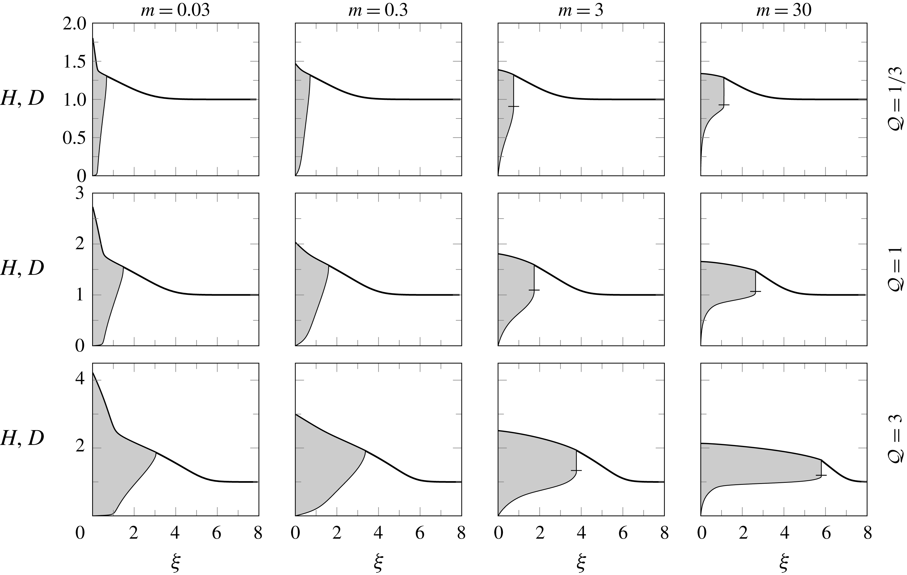
Figure 6 shows a tableau of solutions for a variety of values for
 ${\mathcal{Q}}$
and
 $m$
. We see that for
 $m<3/2$
there are no shocks in the similarity solutions, whilst for
 $m>3/2$
there is a frontal shock. Associated with this discontinuity in the upper-layer thickness, there is also a discontinuity in the gradient of the top surface, and hence the pressure gradient, as this is necessary for a continuous total flux. We note that there is a square-root singularity at the nose for all
 $m$
, which for
 $m>3/2$
joins smoothly onto the vertical shock. Furthermore, we note that for all
 $m$
there is a logarithmic singularity at the origin, which arises from applying lubrication theory at a region where the current is not long and thin and the full two-dimensional Stokes equation should be used. However, this does not affect the shape and spreading of the current beyond a small region near the origin of extent comparable to the thickness. Finally, we observe that for all parameters there is a region of lower-layer fluid extending all the way to the origin, which is a direct consequence of the no-slip boundary condition on the rigid bottom. This is a key distinction from the way Kowal & Worster (Reference Kowal and Worster2015) implemented the bottom boundary condition in their model.
We observe that, as might be expected, larger influx rates
 ${\mathcal{Q}}$
lead to larger radial extents
 $\unicode[STIX]{x1D709}_{\ast }$
and overall a larger total height
 $H$
of the current. Somewhat surprisingly, large changes in
 $m$
have significantly less impact, with the extent
 $\unicode[STIX]{x1D709}_{\ast }$
increasing slightly and the total height
 $H$
decreasing slightly as
 $m$
increases, which is in accordance with global mass conservation.
In the case of a much more viscous upper-layer fluid, i.e. small
 $m$
, we observe a region near the origin, where nearly all the less viscous lower-layer fluid is expelled. At the point where this region ends and the lower layer ceases to be as thin we observe a smooth kink in the top surface.
We observe two further trends: firstly, as the influx
 ${\mathcal{Q}}$
decreases, the top surface flattens except close to the source at the origin; and secondly, as both the influx and viscosity ratio increase, the upper-layer fluid seems to start flowing on top of the lower-layer fluid. In the corresponding limits, these currents are analogous to the flow in a Hele-Shaw cell, where the ‘flat top’ in the gravity current corresponds to the mid-plane between the two rigid boundaries of the Hele-Shaw cell, and to a single-layer gravity current flowing over an approximately rigid lower layer, respectively. These physically motivated limits can be analysed analytically, from which it may be shown that the nose position scales as
 $\unicode[STIX]{x1D709}_{\ast }\sim 1.424{\mathcal{Q}}^{3/8}m^{1/8}$
in the case of a single-layer current as long as
 ${\mathcal{Q}}^{-1}m^{-3}\ll 1\ll {\mathcal{Q}}^{3}m$
, and
 $\unicode[STIX]{x1D709}_{\ast }\sim (2{\mathcal{Q}}{\mathcal{F}}_{crit}^{\prime })^{1/2}$
in the case of a ‘flat top’ current as long as
 ${\mathcal{Q}}\ll m\ll {\mathcal{Q}}^{-3}$
.
Profiles of numerically calculated similarity solutions as functions of the similarity variable
 $\unicode[STIX]{x1D709}$
for influx rates
 ${\mathcal{Q}}\in \{0.1,1,10\}$
and viscosity ratios
 $m\in \{0.03,0.3,3,30\}$
, showing the presence of a frontal shock for
 $m>1.5$
. The horizontal tick shows the height of the shock.

6 Experiments
6.1 Experimental method
Schematic diagram of the experimental set-up. Fluid was injected through a hole in the bottom of a tank such that it spreads radially outwards over the top of a lower layer of fluid. The injected fluid was provided at a constant flow rate by means of a peristaltic pump and was dyed green to allow visualisation of the moving nose of the upper spreading layer.

We conducted a suite of experiments in which one fluid was injected into a pre-existing lower layer of another fluid of equal density, but differing viscosity. A schematic diagram of the experimental apparatus is shown in figure 7. A lower-layer fluid was introduced into a tank of square cross-section 48.5 cm
 $\times$
48.5 cm, with side walls of height 5 cm, and its free surface allowed to become horizontal under gravity. Once the lower layer had attained a uniform height, a density-matched second fluid was injected through a 1 cm diameter hole in the bottom of the tank at a constant flow rate such that the resulting current spread radially outwards over the top of the lower layer. The flow rate of the injected fluid was set by a peristaltic pump and the flux recorded by a mass balance.
Aqueous solutions of glycerol and salt were used for both fluids. The viscosities of the fluids were varied by altering the concentration of glycerol between 0.1 and 2.3 Pa s. A Bohlin rheometer was used to measure the viscosities as functions of temperature and the temperature in the laboratory was carefully monitored throughout the experiments. The densities of the fluids were matched by adding salt, using a hydrometer to measure the densities. In order to enable the detection of the contact between the two fluid layers the injected fluid was dyed green. The evolution of the nose position of the propagating current could then be determined from images.
The axisymmetric profiles of the total thickness of the current,
 $h$
, were determined by digitally imaging the deflection of a line, of approximately 1 mm width, projected onto the top surface of the fluids (titanium dioxide was added to the fluids as an opacifier). The line was imaged using a Nikon D300 camera, with a spatial resolution of 0.21 mm, positioned at an angle
 $\unicode[STIX]{x1D703}=29^{\circ }$
above the horizontal and perpendicular to the projected line. The deflection of the line was measured with respect to a reference image of the projected line on the rigid lower surface with no lower layer, and subpixel accuracy was achieved by fitting a Gaussian profile across the line (see Lister et al. (Reference Lister, Peng and Neufeld2013)). Image analysis was then used to determine the evolution of the total-height profiles of the propagating current. The height and uniformity of the lower layer prior to injection was also checked to within 1 %, using images of the projected line.
To check if lubrication theory is indeed applicable to model these experiments we estimate a modified Reynolds number
 $\mathit{Re}=Q\unicode[STIX]{x1D70C}h_{\infty }/(\unicode[STIX]{x03C0}\unicode[STIX]{x1D707}_{1}r_{hole}^{2})$
, where the velocity scale is assumed to be the vertical outflow velocity through the hole of radius
 $r_{hole}=0.5~\text{cm}$
, and the length scale is assumed to be of the order of the initial height
 $h_{\infty }$
. Using this definition and the values of the physical parameters given in table 1, we find that the Reynolds numbers vary from
 $0.003$
to
 $0.02$
between the experiments. This indicates that the experiments are indeed low-Reynolds-number flows and should be well described by lubrication theory.
Furthermore, we calculate Péclet numbers for the experiments as
 $\mathit{Pe}=\mathit{Sc}\,\mathit{Re}$
, where the Schmidt number is given by
 $\mathit{Sc}=\unicode[STIX]{x1D707}_{1}/(\unicode[STIX]{x1D70C}D_{glycerol})$
. The diffusivity of water in glycerol is estimated to be
 $D_{glycerol}\lesssim 10^{-9}~\text{m}^{2}~\text{s}^{-1}$
(D’Errico et al.
Reference D’Errico, Ortona, Capuano and Vitagliano2004), and therefore
 $\mathit{Sc}\gtrsim O(10^{6})$
. Together with the previous estimates for the Reynolds numbers we conclude that the Péclet numbers vary from
 $5\times 10^{3}$
to
 $3\times 10^{4}$
and hence it is appropriate to neglect the effects of molecular diffusion of glycerol, and hence the viscosity acts as a passive tracer.
In all of the experiments presented here, the viscosity of the lower layer is greater than or equal to the viscosity of the injected fluid
 $\unicode[STIX]{x1D707}_{2}\geqslant \unicode[STIX]{x1D707}_{1}$
, such that
 $m\leqslant 1$
, thereby ensuring that the flow remains axisymmetric. Observations of currents with a less viscous intruding fluid, i.e.
 $m>1$
, show that the interface can become unstable in a manner analogous to the symmetry-breaking viscous fingering instability in Hele-Shaw cells, and the axisymmetric model derived above is no longer applicable for these cases. Experimental measurements of the growth of this instability and a linear stability analysis is beyond the scope of this study and will instead be the focus of a future communication.
The values in each experiment of the initial height
 $h_{\infty }$
, influx
 $Q$
, viscosities
 $\unicode[STIX]{x1D707}_{i}$
and densities
 $\unicode[STIX]{x1D70C}_{1}=\unicode[STIX]{x1D70C}_{2}$
, with uncertainties:
 $\pm 1\,\%$
for
 $h_{\infty }$
;
 $\pm 0.1~\text{cm}^{3}~\text{s}^{-1}$
for
 $Q$
;
 $\pm 5\,\%$
for
 $\unicode[STIX]{x1D707}_{i}$
; and
 $\pm 0.01~\text{g}~\text{cm}^{-3}$
for
 $\unicode[STIX]{x1D70C}_{i}$
. Also, derived quantities such as the viscosity ratio
 $m$
, the non-dimensional influx
 ${\mathcal{Q}}$
and the experimentally measured and numerically computed nose positions,
 $\unicode[STIX]{x1D709}_{\ast }^{exp}$
and
 $\unicode[STIX]{x1D709}_{\ast }^{num}$
respectively, and their relative deviation
 $\unicode[STIX]{x0394}\unicode[STIX]{x1D709}_{\ast }$
. The values
 $\unicode[STIX]{x1D709}_{\ast }^{exp}$
were obtained from performing a least-squares fit to the time series of measured values of
 $r_{\ast }(t)$
.

6.2 Comparison of theory and experiments
We first check whether the measured current spreads in a self-similar manner. The experimental measurements show that, with the similarity variable given by (2.10), the profiles of the top surface collapse well onto a self-similar shape, thus supporting the application of the theory developed above. A representative example of this collapse is shown in figure 8.
Figure 9 compares both the self-similar total-height profiles
 $H(\unicode[STIX]{x1D709})$
obtained from the numerical calculations with the measurements from the experiments. The theory captures the trend of the top-surface profiles very well over a wide range of influxes
 ${\mathcal{Q}}$
and viscosity ratios
 $m<1$
and reproduces most features of the flow. In particular, the experiments demonstrate the same trend as observed in the numerical calculations: with increasing influx,
 ${\mathcal{Q}}$
, the pre-existing fluid layer plays an smaller role such that the injected fluid forms a more compact current, with a sharp, distinct nose. As also predicted by the model, the viscosity ratio
 $m$
has a significantly smaller effect on the shape of the current than the effect of changes in the influx
 ${\mathcal{Q}}$
. For several values of
 ${\mathcal{Q}}$
and
 $m$
, a small bump is observed between the nose and origin in the experiments, but is absent from the numerical calculations. The cause of the bump is not clear, but it seems to have little effect on the overall profile.
In figure 10 and table 1 we compare the nose positions
 $\unicode[STIX]{x1D709}_{\ast }$
as measured in the experiments with the values calculated using the model above, which reveals a fairly good fit with relative deviations in the range of 5 to 20 %. The trend is again captured very well, especially considering the simplifying assumptions made, the difficulty resolving the exact nose position from the colour change, and the uncertainties in the physical parameters. Again, both the experimental data and the numerical model show that the nose position depends mainly on the influx
 ${\mathcal{Q}}$
with only a comparatively small variation with the viscosity ratio
 $m$
. In particular, both the numerical calculations and the experimental data seem to be approaching the correct asymptotics
 $\unicode[STIX]{x1D709}_{\ast }\sim {\mathcal{Q}}^{1/2}$
as
 ${\mathcal{Q}}\rightarrow 0$
and
 $\unicode[STIX]{x1D709}_{\ast }\sim {\mathcal{Q}}^{3/8}$
as
 ${\mathcal{Q}}\rightarrow \infty$
.
Overall, the agreement of the numerical and the experimental results suggests that the theory captures the relevant physical processes involved and gives a good description of the experimental results.
(a) The measured profiles plotted every 10 s for experiment No.
 $1$
. (b) The same profiles as functions of the similarity variable
 $\unicode[STIX]{x1D709}$
. A similar collapse is observed in the other experiments.

Measured (solid) and computed (dotted) heights
 $H$
and
 $D$
as functions of
 $\unicode[STIX]{x1D709}/\unicode[STIX]{x1D709}_{\ast }^{num}$
, so the similarity variable is rescaled by the numerical nose position. The values of
 ${\mathcal{Q}}$
and
 $m$
are as in table 1.

Log–log plot of the measured (symbols) and computed (curved lines) nose positions,
 $\unicode[STIX]{x1D709}_{\ast }^{exp}$
and
 $\unicode[STIX]{x1D709}_{\ast }^{num}$
, respectively, as functions of
 ${\mathcal{Q}}$
and rescaled by
 ${\mathcal{Q}}^{1/2}$
with
 $m$
fixed. The predicted asymptotic dependence on
 ${\mathcal{Q}}$
for large and small
 ${\mathcal{Q}}$
is
 $\unicode[STIX]{x1D709}_{\ast }\sim {\mathcal{Q}}^{3/8}$
and
 $\unicode[STIX]{x1D709}_{\ast }\sim {\mathcal{Q}}^{1/2}$
respectively (thin straight lines). The experimental data can be found in table 1.

7 Discussion and conclusions
The axisymmetric spread of a viscous gravity current over a uniform layer of a second fluid of equal density has been analysed theoretically and using laboratory experiments. Through the application of lubrication theory, we derived evolution equations for the top surface and the fluid–fluid interface. In this framework a self-similar rescaling was found that is a function of three non-dimensional parameters: the ratio of fluid viscosities,
 $m$
; the relative density difference,
 $\unicode[STIX]{x1D700}$
; and a non-dimensional influx,
 ${\mathcal{Q}}$
, defined in (2.14) from the dimensional influx rate, the pre-wetting film thickness and the fluid properties.
In the limit of equal densities,
 $\unicode[STIX]{x1D700}\rightarrow 0$
, the interfacial slope no longer contributes to the hydrostatic pressure gradient in the lower-layer fluid and therefore the nature of the flow and the interfacial evolution changes. Mathematically,
 $\unicode[STIX]{x1D700}\rightarrow 0$
is a singular limit of the governing equations in which the equation for the depth ratio,
 $\unicode[STIX]{x1D706}$
, changes from a parabolic advection–diffusion equation (Lister & Kerr Reference Lister and Kerr1989) to a hyperbolic pure advection equation.
As a consequence of the hyperbolic feature of the governing equations for equal densities, the solutions are no longer intrinsically smooth and, instead, vertical discontinuities, or shocks, can form on the interface. We find that these form for a sufficiently less viscous upper-layer fluid and that the critical viscosity ratio for this transition is
 $m_{crit}=3/2$
. This transition can be understood by noting that, for a given pressure gradient, the average upper-layer fluid velocity increases with the relative upper-layer thickness, since, although more of the upper-layer fluid is closer to the no-slip bottom, more of the whole flow is the less viscous fluid.
Reintroducing a small density difference between the fluids,
 $0<\unicode[STIX]{x1D700}\ll 1$
, regularises the equations near the nose and, by analytically solving for local travelling-wave solutions, we obtain a shock condition commonly known as the Oleinik entropy condition. This regularisation justifies the assumptions of a long thin current. Further analysis reveals that for
 $m>3/2$
the self-similar solution has a frontal shock with relative height
 $\unicode[STIX]{x1D706}_{crit}(m)$
, which is the maximal shock height allowed under the Oleinik entropy condition.
We note that, whilst large variations of
 ${\mathcal{Q}}$
have a proportionately large effect on the shape and spreading rate of the current, variations of the viscosity ratio, somewhat surprisingly have a significantly smaller impact.
The numerical solutions also provide a connection both to single-layer gravity currents (e.g. Huppert Reference Huppert1982b
) in either the limit of large influx rates (
 ${\mathcal{Q}}\rightarrow \infty$
) or of very viscous lower layers (
 $m\rightarrow \infty$
), and to the flow in a constant-width Hele-Shaw cell (e.g. Yang & Yortsos Reference Yang and Yortsos1997) in the limit of small influx rates (
 ${\mathcal{Q}}\rightarrow 0$
).
To test these theoretical predictions, we also carried out laboratory experiments measuring both the top-surface profile and the radial extent of the current using two density-matched aqueous solutions of glycerol. These experiments confirmed that the evolution of the current is self-similar. Furthermore, we found good agreement between the experiments and theoretical predictions for the top-surface shape and the nose position as function of
 ${\mathcal{Q}}$
and
 $m$
, suggesting that the essential physics is captured by the theoretical model.
The shocks which we found in equal-density two-layer viscous gravity currents can be contrasted to some more-familiar shocks found in other hyperbolic systems, such as those in gas dynamics and in hydraulic jumps (e.g. Billingham & King Reference Billingham and King2001). In these cases the shocks are known as classical shocks and their evolution is constrained by an entropy condition which allows characteristics only to enter the shock and not to leave it; thus initial conditions with characteristics diverging from an initial discontinuity yield an expansion fan rather than a shock. On the other hand, in non-classical shocks characteristics can leave the shock and hence the shock conditions must be determined by locally resolving some regularising mechanism near any shock discontinuity (see, for example, Jacobs, McKinney & Shearer Reference Jacobs, McKinney and Shearer1995).
The shocks found in equal-density gravity currents and in Hele-Shaw cells, are both examples of non-classical shocks which are, in these cases, related to a non-convex relationship between the relative thickness of the intruding fluid and the corresponding relative flux of intruding fluid, i.e. the flux function
 ${\mathcal{F}}(\unicode[STIX]{x1D706})$
. In fact, the systems are governed by the same flux function and hence the critical viscosity ratio
 $m_{crit}=3/2$
is the same in two-layer viscous gravity currents and in equal-density miscible two-fluid flow in a Hele-Shaw cell (Yang & Yortsos Reference Yang and Yortsos1997; Lajeunesse et al.
Reference Lajeunesse, Martin, Rakotomalala and Salin1997, Reference Lajeunesse, Martin, Rakotomalala, Salin and Yortsos1999, Reference Lajeunesse, Martin, Rakotomalala, Salin and Yortsos2001).
However, for the shocks occurring in equal-density gravity currents, there is a simple regularisation given small density differences as described above, making them one-sided characteristic shocks. In comparison, the shocks in flows in a Hele-Shaw cell are thought to be regularised by the much more complicated two-dimensional Stokes equations (Yang & Yortsos Reference Yang and Yortsos1997). In fact, laboratory experiments (Petitjeans & Maxworthy Reference Petitjeans and Maxworthy1996) and numerical simulations (Chen & Meiburg Reference Chen and Meiburg1996; Rakotomalala et al. Reference Rakotomalala, Salin and Watzky1996) suggest that, in a Hele-Shaw cell, the shock heights exceed the maximal shock height permitted by the Oleinik entropy condition, making them undercompressive shocks.
The existence of a solvable regularisation and therefore of simple shock conditions significantly facilitates any future analysis in the case of two-layer gravity currents, such as, for example, a linear stability analysis along the lines of Mathunjwa & Hogg (Reference Mathunjwa and Hogg2006). A natural extension of the work presented here is the stability of the interface for
 $m>3/2$
. In the comparable problem of miscible flow in a Hele-Shaw cell this is known to be unstable (Wooding Reference Wooding1969). Indeed, in some further exploratory experiments we have conducted, for
 $m>3/2$
there is the suggestion of a new and complex fingering pattern arising from the instability of the interface. We anticipate that the vertical shocks and the associated jumps in pressure gradient play a crucial role in the instability mechanism, as has been suggested for the flow in a Hele-Shaw cell by (Lajeunesse et al.
Reference Lajeunesse, Martin, Rakotomalala and Salin1997, Reference Lajeunesse, Martin, Rakotomalala, Salin and Yortsos1999, Reference Lajeunesse, Martin, Rakotomalala, Salin and Yortsos2001) or Bischofberger et al. (Reference Bischofberger, Ramachandran and Nagel2014).
Acknowledgements
T.-F.D. gratefully acknowledges an Engineering and Physical Sciences Research Council studentship. J.A.N. acknowledges support from a Royal Society University Research Fellowship. All data accompanying this publication are directly available within the publication.
Appendix A. Two-dimensional geometry
A two-dimensional two-layer current with upper-layer volume
 $V_{2D}=Qt^{1/2}$
behaves similarly to the axisymmetric currents with upper-layer volume
 $V_{axi}=Qt$
that we have analysed in the body of the paper. In both cases a balance between influx and spreading allows for a similarity solution in which the upper layer is characterised by a constant thickness (see appendix B of Lister & Kerr (Reference Lister and Kerr1989)). We sketch here the similarities and differences between the 2-D and axisymmetric analyses.
In two dimensions the relevant similarity variable and non-dimensional influx are given by
 $$\begin{eqnarray}\displaystyle & \displaystyle \unicode[STIX]{x1D709}=xt^{-1/2}\left(\frac{3\unicode[STIX]{x1D707}_{2}}{\unicode[STIX]{x1D70C}_{1}gh_{\infty }^{3}}\right)^{1/2}, & \displaystyle\end{eqnarray}$$
 $$\begin{eqnarray}\displaystyle & \displaystyle {\mathcal{Q}}=\left(\frac{3\unicode[STIX]{x1D707}_{2}Q^{2}}{16\unicode[STIX]{x1D70C}_{1}gh_{\infty }^{5}}\right)^{1/2}. & \displaystyle\end{eqnarray}$$
Since
 $\unicode[STIX]{x1D709}\propto t^{1/2}$
in both (2.10) and (A 1), the depth-integrated, mass-conservation equations in two dimensions
 $$\begin{eqnarray}\displaystyle & \displaystyle H_{\unicode[STIX]{x1D70F}}-{\textstyle \frac{1}{2}}\unicode[STIX]{x1D709}H_{\unicode[STIX]{x1D709}}+(q_{H})_{\unicode[STIX]{x1D709}}=0, & \displaystyle\end{eqnarray}$$
 $$\begin{eqnarray}\displaystyle & \displaystyle D_{\unicode[STIX]{x1D70F}}-{\textstyle \frac{1}{2}}\unicode[STIX]{x1D709}D_{\unicode[STIX]{x1D709}}+(q_{D})_{\unicode[STIX]{x1D709}}=0, & \displaystyle\end{eqnarray}$$
 $q_{H}$
and
 $q_{D}$
. With the choice of non-dimensional influx, (A 2), the boundary conditions are identical to (2.13).
The fluxes
 $q_{H}$
and
 $q_{D}$
are the same as in the axisymmetric case (2.12), since the local analysis of the piece-wise parabolic velocity profiles is not influenced by the global geometry. Therefore, we recover the same flux function
 ${\mathcal{F}}$
, (3.2a
). This implies in particular that the local analysis of the regularisation of any shock via travelling-wave solutions is identical in the two geometries. Therefore, we obtain shocks if and only if
 $m>3/2$
, which have to obey the Oleinik entropy condition (3.10), and in the steady self-similar case a frontal shock is found with height
 $\unicode[STIX]{x1D706}_{crit}$
defined by (3.12).
As a final remark, in the 2-D case the origin is non-singular, and solutions do not exhibit the logarithmic singularity which occurs in the axisymmetric case. Nonetheless, the boundary condition (2.13b
) is still automatically satisfied as before, due to a similar argument as at the end of § 4.3. Numerical integration shows that the behaviour of the solutions is largely similar between the two different geometries except the mentioned singularity at the origin in the axisymmetric case. A tableau of 2-D solutions for a range of values for
 ${\mathcal{Q}}$
and
 $m$
is shown in figure 11.
Profiles of numerically calculated similarity solutions as functions
 $\unicode[STIX]{x1D709}$
for influx rates
 ${\mathcal{Q}}\in \{1/3,1,3\}$
and viscosity ratios
 $m\in \{0.03,0.3,3,30\}$
in the case of 2-D geometry, again showing the appearance of shocks for
 $m>1.5$
but without the singularity at the origin. The horizontal tick shows the height of the shock.