2.1 Measurement methodology

(a) Time-resolved PIV. The complex flow structures and intricate instabilities exhibited by swirling flows mandate time-resolved measurements for fundamental insights. The measurement tools can be chosen on the basis of their dynamic response to the fluid flows. The most widely used tools in fluid flows include hot wire anemometry (HWA), laser Doppler anemometry (LDA) and PIV (Adrian Reference Adrian1991; Tropea, Yarin & Foss Reference Tropea, Yarin and Foss2007; Albrecht et al. Reference Albrecht, Damaschke, Borys and Tropea2013), to name a few. Among these, PIV receives special attention because of its planar measurement features (Sung & Yoo Reference Sung and Yoo2001; Schröder et al. Reference Schröder, Geisler, Staack, Elsinga, Scarano, Wieneke, Henning, Poelma and Westerweel2011), unlike LDA and HWA where measurements are pointwise. The arrangement involved in time-resolved PIV is schematically shown in figure 3(a,b). The arrangement includes a high-speed laser (illumination source) and an imaging system (camera) positioned in an orthogonal manner.

Figure 3.

(a) Schematic showing the arrangement of the different optical diagnostic systems. (b) Time-resolved PIV set-up. (c) High-speed shadow imaging system.

The laser used here is of high-repetition-rate (10 kHz) dual-pulse Nd:YLF type, with a pulse energy of $30~\text{mJ}~\text{pulse}^{-1}$ at an emission wavelength of 527 nm (make: Photonics Inc.). A flexible guiding arm is employed to direct the cylindrical laser beam towards the measurement section. Furthermore, the cylindrical beam is converted to a thin sheet ( ${\sim}$ 1 mm) with the help of sheet optics (see figure 3 a). The focal length $f$ of the sheet optics is chosen as $-$ 10 mm, to ensure an optimum aperture angle $\unicode[STIX]{x1D6FC}$ to illuminate the desired spatial dimensions of the flow field. In this study, PIV is carried out in two ways. In the first case, PIV is performed only in the gas phase (i.e. without the presence of droplets). In the second case, the flow field in the presence of droplets is imaged. In both cases, only the gas phase is seeded with diethyl hexyl sebacate (DEHS; oil density $\unicode[STIX]{x1D70C}=912~\text{kg}~\text{m}^{-3}$ ) as tracer particles. The diameter ( ${\sim}1{-}3~\unicode[STIX]{x03BC}\text{m}$ ) of tracer particles is chosen in such a way as to maintain tracing accuracy error of less than 1 %. During PIV measurements in the presence of droplets, it is important to minimize the influence of tracer particles in droplet breakup and other related processes (Khalitov & Longmire Reference Khalitov and Longmire2002; Kosiwczuk et al. Reference Kosiwczuk, Cessou, Trinite and Lecordier2005). To validate this, comparison is made between PIV raw images recorded in the presence of both droplets and tracer particles, as well as only with droplets. There is no significant difference in the breakup process, which confirms negligible influence of the tracer particles. In addition, for a given incident laser excitation, the intensity of light scattered by the water droplets is much higher than that by the DEHS particles. This is because the initial size of the injected water droplets ( $d_{o}=500~\unicode[STIX]{x03BC}\text{m}$ ) is much higher than that of the DEHS particles ( ${\sim}1{-}3~\unicode[STIX]{x03BC}\text{m}$ ), leading to larger scattering cross-sections. This characteristic feature enables to us distinguish the droplets from the DEHS particles in the raw images.

The light scattered by the DEHS particles and droplets is recorded with a Photron SA5 high-speed camera (maximum imaging rate is $7000~\text{frames}~\text{s}^{-1}$ at 1024 pixel $\times$ 1024 pixel resolution). The camera and laser units are controlled with a programmable tuning unit (PTU) to ensure effective synchronization. In addition, an optical bandpass filter of 527 nm is attached in front of the camera lens to avoid any noisy scattering signals due to the ambient. Images are acquired in double-frame mode with an optimal time interval d $t$ between two images. Further details on the steps involved in identifying the optimal d $t$ , tracer particles and other PIV measurement settings can be found in Keane & Adrian (Reference Keane and Adrian1990) and Raffel et al. (Reference Raffel, Willert, Wereley and Kompenhans2013).

Across all the flow conditions, images are acquired at 3.5 kHz ( $3500~\text{frames}~\text{s}^{-1}$ ) with an acquisition time of 0.59 s (i.e. 2000 images are acquired for each case). Superior spatial resolution is ensured by employing a magnification factor of ${\sim}$ 10.24 ( $10~\text{pixels}~\text{mm}^{-1}$ ) with a field of view (FOV) of 100 mm $\times$ 100 mm.

The vector fields are reconstructed from the recorded double-frame raw images using a commercial PIV postprocessing package (Davis 8.3; make: Lavision GmbH). The vector field calculation is carried out using a cross-correlation technique with a multipass decreasing window size (the final interrogation window size is 48 pixel $\times$ 48 pixel). The choice of interrogation window size (i.e. 48 pixel $\times$ 48 pixel) is arrived at based on the peak correlation value (0.8–0.9) inside the field of view.

The accuracy of the PIV measurements is highly dictated by the laser sheet thickness $(\unicode[STIX]{x1D6FF}_{t})$ , the time delay between two pulses $(\text{d}t)$ , the particle displacement $(\unicode[STIX]{x1D6FF}s)$ and the number of particles $(N)$ per interrogation window. The correctness of the abovementioned parameters is validated by performing uncertainty analysis using the ‘correlation statistics’ method. This method attempts to compute the disparity between the correlation peaks observed across two images. The uncertainty in the velocity $(\boldsymbol{u}_{\boldsymbol{e}\boldsymbol{r}\boldsymbol{r}\boldsymbol{o}\boldsymbol{r}})$ values is computed based on the positional disparity observed across two peaks. In the present study, the uncertainty in the velocity is found to be $\pm$ 1 % of the local velocity value. Further details about this method can be found in Sciacchitano, Wieneke & Scarano (Reference Sciacchitano, Wieneke and Scarano2013) and Wieneke (Reference Wieneke2015).

(b) High-speed shadow imaging. The near-field (i.e. locations close to the initial interaction) droplet breakup mechanism and vortex–droplet interactions are visualized using a high-speed shadow imaging system. The optical arrangement involves in the same plane mounting of a high-pulse-rate (100 kHz) LED strobe lamp (make: IDT vision) and a high-speed camera in the same plane (see figure 3 a,c). A diffuser plate is positioned in front of the strobe lamp to ensure uniform background light intensity. Furthermore, the camera shutter and strobe lamp flash duration are synchronized via a delay generator to yield time frozen images of the droplets.

For near-field imaging, a long-distance microscope (make: Questar; QM1 model) with a zoomed-in field of view of 10 mm $\times$ 10 mm is coupled to the high-speed camera. This arrangement ensures a relatively high spatial resolution (i.e. magnification factor ${\sim}75~\text{pixels}~\text{mm}^{-1}$ ). Images are acquired at $7500~\text{frames}~\text{s}^{-1}$ with an exposure time of $1/7500~\text{s}$ . The acquisition time is chosen as 0.67 s (i.e. 5000 images per experimental realization).

2.2 Flow parameters and test conditions

The experiments are globally characterized using two major non-dimensional numbers, the liquid and gas phase Reynolds numbers $(Re_{g},Re_{l})$ , and the momentum ratio ( $MR$ ). These two parameters represent global flow conditions, whereas the local droplet–vortex interaction dynamics is characterized by the Weber number defined based on the vortex strength $(We)$ (to be explained later),

Here, the parameters $\unicode[STIX]{x1D70C}$ , $\unicode[STIX]{x1D707}$ and $U$ are the density, the viscosity and the bulk exit velocity of the fluids used, where ‘ $g$ ’ and ‘ $l$ ’ stand for the gas and liquid phases respectively. Since the airflow is routed through the swirler, it is customary to define an effective diameter $D_{s,eff}$ to account for the vanes and hub in the flow path. In most previous works, the area ratio $(A_{s,eff}/A_{o})$ is not included in the calculation of $MR$ . In those cases, $MR$ is viewed as the dynamic pressure ratio between two coflowing fluids. Few researchers (Engelbert, Hardalupas & Whitelaw Reference Engelbert, Hardalupas and Whitelaw1995; Lozano et al. Reference Lozano, Barreras, Siegler and Löw2005) have explicitly included the area ratio for precise representation of the momentum transfer across the two fluids. For instance, if the area ratio is not included in (2.3), the calculated value of $MR$ for all of the flow cases shown in table 1 is found to be ${<}$ 1, which implies a weak interaction between the droplets and the flow. However, the experimental observations show different trends, i.e. significant coupling (one-way and two-way) for almost all of the airflow rates.

Further, it should be noted that the term $U_{l}$ in (2.2) is the bulk liquid jet velocity at the nozzle exit before it breaks up into droplets. Here, $U_{l}$ is evaluated based on the mass conservation principle. In addition, the axis length scales ( $y,r$ ) are non-dimensionalized with the swirler outer annulus radius ( $R_{o}$ ). The experimental flow conditions are compiled in table 1.

Table 1.

Experimental test cases.

LG–GL, liquid to gas and gas to liquid two-way coupling; G–L, transition to one-way gas to liquid coupling; GL, strong one-way gas to liquid coupling.

3.1 Global swirling flow field in the absence of droplets

The global features of the flow field are elucidated on the basis of vector fields reconstructed from the PIV raw images. It is mandatory to analyse the gas phase flow field in the absence of droplets across all flow rates since the droplet interaction is expected to be a strong function of $MR$ . The time-averaged flow fields obtained for different airflow rates are shown in figure 4. For brevity, only three flow conditions ( $C2$ , $C4$ , $C7$ ) are shown in figure 4(a). The remaining data can be found in the supplementary material (§ 1, figure S1) available at https://doi.org/10.1017/jfm.2017.495. It should be noted that the flow field looks identical in a topological sense for all cases (figure 4), irrespective of airflow rate. This feature can be elucidated by invoking the definition of swirl number ( $S_{G}$ ), which embodies the ratio between the axial flux of tangential momentum and the axial flux of axial momentum,

Beér & Chigier (Reference Beér and Chigier1972) showed that for a flat vane swirler, the ratio between the two fluxes (tangential and axial) is geometry-dependent and remains constant irrespective of the flow rate. Hence, (3.1) can be rewritten as

where $d_{o}$ and $d_{h}$ are the swirler outer and inner hub diameters.

In the present experiments, the swirl number ( $S_{G}$ ) is found to be 0.81, which represents a strong swirling jet (figure 3 b). Detailed information regarding the spatial regimes of the abovementioned flow configuration can be found in Rajamanickam & Basu (Reference Rajamanickam and Basu2017).

3.2 Global response of the swirling flow field in the presence of droplets

The alterations of the flow field in the presence of droplets with respect to different injection locations (OSL 1–3, ISL 1–3) are shown in figure 7 and figure S3. To elucidate the topological modifications, the flow field involving only droplets (i.e. $MR=0$ ) is also shown in figure 7(a). From a global viewpoint, it is seen that at very low airflow rates (i.e. $MR=185$ , $Re_{g}=5089$ ), the injected droplets penetrate inside the vortex core region, which results in complete alteration of the flow field (see the first column in figure 7 b,d and figure S3). In these conditions, substantial momentum is transferred from the liquid to the gas phase, leading to flow variations. On the other hand, slight variation is observed in the droplet trajectories (shown later), without any major breakup event. This situation represents two-way coupling between the droplets and the swirling gas phase (denoted as LG–GL coupling (i.e. liquid to gas, gas to liquid)). However, at high airflow rates $(14\,000<Re_{g}\leqslant 33\,888,1920<MR\leqslant 8164)$ , the swirling gas flow predominantly transfers momentum to the liquid droplets, leading to different forms of breakup and dispersion (to be explained later). Here, the flow field (see the second and third columns in figure 7 b,d) resembles the one shown in figure 3(a). This is identified as one-way gas to liquid coupling (GL coupling). Hence, with the increase in the airflow rate, a transition is observed from two-way LG–GL to one-way GL coupling. This G–L coupling transition occurs at $(Re_{g}\sim 7965,MR\sim 450)$ , where the effect of droplets on the flow field starts to become insignificant in a global sense.

The gas phase flow fields for OSL and ISL injection are largely unaltered for high $MR$ , except that there is slight deformation of the vortex core in certain local regions (shown as white dotted lines in figure 7 bi,ii). On account of this, slight change in orientation is observed for the vector fields (see figure 7 c). In particular, for injections corresponding to upstream of the vortex core (OSL 1), significant alteration of the vector field is detected. For instance, the deviation angle $\unicode[STIX]{x1D6FC}$ subtended by the velocity vectors for OSL 1 ( $y/R_{o}=0.5$ ) (figure 7 c) is found to be as high as $39^{\circ }$ . Interestingly, the vector field deformation is much more pronounced in the recirculation zone (VBB). For these injection locations (OSL 1, OSL 2), the vortex core rotation is abruptly disturbed, leading to change in the orientation of the flow direction. This effect is not observed for the $y/R_{o}=1.5$ location, because of the downstream nature of the injection (i.e. position away from the vortex core); in essence, the vortex core experiences negligible impact from the injected droplets (figure 7 b,c). In addition, the vortex core remains unaltered for all injection locations at the ISL. This yields a similar flow field irrespective of the injection location (ISL 1–3). Hence, in figure 7(d), only the flow field pertaining to ISL 1 is shown; the others (ISL 2, 3) can be found in figure S3(ii),(iii).

The fundamental response between the gas phase vortices and the liquid droplets can be explained by a simple force balance model (see figure 8 a). The parameter $\unicode[STIX]{x1D709}$ , which defines the dynamic pressure ratio between the two phases (3.3) is used as a criterion to understand this phenomenon. The dynamic pressure ratio $\unicode[STIX]{x1D709}$ is the parameter that quantifies momentum transfer pathways between two coflowing fluids. For example, in situations where $\unicode[STIX]{x1D709}<1$ , (3.3) represents the momentum transfer occurring from the liquid to the gas phase (i.e. LG coupling). The airflow rate pertaining to $\unicode[STIX]{x1D709}\sim 1$ is delineated as the transition condition, followed by strong one-way gas phase coupling when $\unicode[STIX]{x1D709}\gg 1$ (i.e. GL coupling).

Here, $V_{\unicode[STIX]{x1D714}}$ represents the velocity induced by vortices. It can be written in terms of the space–time-averaged circulation strength $(\overline{\unicode[STIX]{x1D6E4}})$ as $V_{\unicode[STIX]{x1D714}}=\overline{\unicode[STIX]{x1D6E4}}/2\unicode[STIX]{x03C0}r$ , where $r$ is the vortex core radius, which is calculated from a time-averaged streamline plot obtained from PIV. The steps involved in calculation of the circulation strength $\overline{\unicode[STIX]{x1D6E4}}$ from the vorticity magnitude will be explained later in great detail. The droplet velocity $V_{d}$ is acquired from PIV without coflowing swirl air (i.e. $MR=0$ ). For $0<Re_{g}<7164$ , the value of $\unicode[STIX]{x1D709}$ is found to be less than 1, which shows that the effect of $\overline{\unicode[STIX]{x1D6E4}}$ is minimal and injected droplets penetrate inside the vortex core (figure 8 b). On the other hand, increased circulation strength $\overline{\unicode[STIX]{x1D6E4}}$ at $7164\leqslant Re_{g}\leqslant 33\,888$ causes $\unicode[STIX]{x1D709}\gg 1$ , which acts as a barrier to droplet penetration. As mentioned earlier, the deflection caused to the vortex eye for $x/R_{o}=2.5$ (OSL) is due to direct impact of droplets on the vortex centre (figure 8 c). However, the opposite effect is observed for $x/R_{o}=0.7$ (ISL); here, the injected droplets first interact with the recirculation zone, resulting in upward motion of the droplets. This phenomenon prevents direct impact of droplets on the right side of the vortex core, resulting in a virtually unaltered flow field (figure 8 d).

Since, in these experiments, the liquid phase flow rate is maintained constant, the only variable that governs the dynamic pressure ratio $\unicode[STIX]{x1D709}$ is the circulation strength of the vortex (i.e. $=f(\overline{\unicode[STIX]{x1D6E4}})$ ). Hence, the control parameter that defines this global modification is $\overline{\unicode[STIX]{x1D6E4}}$ . The circulation strength $\overline{\unicode[STIX]{x1D6E4}}$ corresponding to the transition flow condition $(Re_{g}\sim 7965,MR\sim 450)$ is identified as critical $\overline{\unicode[STIX]{x1D6E4}}_{c}$ .

3.3 Global response of droplets in the swirling gas flow field

The results shown in the previous section outline how the global flow field is modified in the presence of the droplets. Here, we describe how the droplets respond to the swirling flow field (at both the OSL and the ISL). Once again, the results shown here are intended only for quantifying the global parameters. The detailed droplet–vortex interaction and breakup dynamics will be explained later using a high-speed shadow imaging technique.

To illustrate the dynamics, only droplet images are extracted from the PIV raw images, and the image processing steps involved with this are shown in figure S4.

The global response of the droplets on interaction with the vortical structures is shown in figure 9. Here, only two extreme cases are shown (i.e. one for OSL and the other for ISL injection, i.e. OSL 2 and ISL 2) across three flow conditions ( $MR=185$ , 450, 8164). From the droplet perspective, the acquired images show LG–GL coupling ( $MR=185$ ) with the vortex (see figure 9ii). The droplet pathways are altered but not in a significant fashion. Similarly, in transition flow conditions ( $MR\sim 450$ ), the increased circulation strength imposed by the vortex results in a strong interaction between the droplet and the swirling flow field (G–L). As a result, the droplet trajectory deviates from its straight path by an angle $\unicode[STIX]{x1D703}^{\prime }$ (spatially averaged instantaneous angle, shown as red dotted lines in figure 9iii–vi) along with significant spatial dispersion (explained in detail in later sections). The magnitude of the dispersion increases with the momentum ratio ( $MR$ ), as evidenced in figure 9(iv) and (vi). The global observations can be summarized as follows:

1. (1) $0<Re_{g}<7164,0<MR<450\rightarrow \overline{\unicode[STIX]{x1D6E4}}<\overline{\unicode[STIX]{x1D6E4}}_{c}\rightarrow$ two-way LG, GL coupling (movie 2);

2. (2) $Re_{g}\approx 7164,MR\approx 450\rightarrow \overline{\unicode[STIX]{x1D6E4}}\sim \overline{\unicode[STIX]{x1D6E4}}_{c}\rightarrow$ transition to one-way GL coupling (movie 3);

3. (3) $7164\leqslant Re_{g}\leqslant 33\,888,450\leqslant MR\leqslant 8164\rightarrow \overline{\unicode[STIX]{x1D6E4}}\geqslant \overline{\unicode[STIX]{x1D6E4}}_{c}\rightarrow$ strong one-way GL coupling (movie 4).

To precisely locate the transition, experiments were carried out for three to four flow rates ( $MR=365$ , 402, 420) close to the transition state. Strictly speaking, the transition does not pertain to a particular value, rather it is observed over a range. In the present experiments, we observed the transition in the range of $420\leqslant MR\leqslant 460$ . However, for simplicity we have considered $MR\sim 450$ as a representative critical/transition flow condition.

In a nutshell, $\overline{\unicode[STIX]{x1D6E4}}$ is the forcing parameter induced by the vortex strength, which will predominantly determine the global response $\unicode[STIX]{x1D703}^{\prime }$ of the droplet. The absolute values for $\overline{\unicode[STIX]{x1D6E4}}$ and $\unicode[STIX]{x1D703}^{\prime }$ will be shown in later sections.

Figure 9.

Sample instantaneous visualization of droplet trajectories: (i), (ii) droplet trajectories at low $MR$ ; (iii), (iv) droplets injected at the OSL (OSL 2) at medium to high $MR$ ; (v), (vi) droplets injected at the ISL (ISL 2) at medium to high $MR$ .

Figure 10.

The coherence function $C_{\unicode[STIX]{x1D6E4}^{\prime },\unicode[STIX]{x1D703}^{\prime }}(f)$ (a) evaluated for droplets injected at the OSL and (b) evaluated for droplets injected at the ISL: (i) OSL 1, ISL 1; (ii) OSL 2, ISL 2; (iii) OSL 3, ISL 3.

4.1 Coherence analysis

The essential role of coherence analysis is to estimate the relationship between the input $x(t)$ and output $y(t)$ signal in a linear time invariant system. Mathematically, it is defined as the ratio between the cross-spectral density of $x(t),y(t)$ and the auto spectral density of $x(t),y(t)$ (Bendat & Piersol Reference Bendat and Piersol1980). The coherence value can vary from 0 to 1; the higher the coherence value is (i.e. closer to unity), the greater the chance of linearity between the two signals:

In the present experiments, $x(t)$ and $y(t)$ are $\unicode[STIX]{x1D6E4}^{\prime }$ and $\unicode[STIX]{x1D703}^{\prime }$ respectively; hence, equation (4.1) can be written as

The coherence function $C_{\unicode[STIX]{x1D6E4}^{\prime },\unicode[STIX]{x1D703}^{\prime }}(f)$ evaluated for different injection locations across various flow rates is presented in figure 10. On account of the LG–GL interaction (mostly liquid to flow), coherence values $C_{\unicode[STIX]{x1D6E4}^{\prime },\unicode[STIX]{x1D703}^{\prime }}(f)$ are not evaluated for $0<MR<450$ . The results pertaining to $MR>450$ are depicted in figure 10(a) for droplets injected at the OSL. It is seen that for all three axial positions, higher coherence ( ${\sim}$ 0.85) is observed around 80–100 Hz. Although the coherence value decays drastically at higher frequencies, interestingly, there is a second peak in $C_{\unicode[STIX]{x1D6E4}^{\prime },\unicode[STIX]{x1D703}^{\prime }}(f)$ for frequencies around 600–900 Hz. In particular, these values are higher for downstream injection locations (i.e. OSL 3; figure 10 aiii). This indicates that the interaction between $\unicode[STIX]{x1D6E4}^{\prime }$ and $\unicode[STIX]{x1D703}^{\prime }$ in the OSL (for OSL injections described earlier) is coupled in two frequency bands, namely the primary ( $f_{p}$ ) and secondary ( $f_{s}$ ).

On the contrary, the dispersion of droplets injected at the ISL (figure 10 b; ISL injections) is predominantly coupled with the local circulation in a narrow frequency band (80–100 Hz) exhibiting very high coherence values of ${\sim}0.85{-}0.9$ . These two contradictory behaviours between the OSL and the ISL indicate radical changes in the interaction dynamics. In both cases (OSL and ISL injections), the transition flow condition is coupled only in a single frequency range (no second peak) and also exhibits low coherence, $C_{\unicode[STIX]{x1D6E4}^{\prime },\unicode[STIX]{x1D703}^{\prime }}(f)\sim 0.2{-}025$ (figure 10 a,bi).

5.1 Spatial eigenmodes of the gas flow field

Proper orthogonal decomposition can be implemented in two ways, classical POD and the method of snapshots (Sirovich Reference Sirovich1987). The latter one has received greater attention in analysing turbulent flows (Berkooz, Holmes & Lumley Reference Berkooz, Holmes and Lumley1993). Mathematically, POD decomposes the fluctuation in velocity components $(u^{\prime },v^{\prime })$ into spatial ( $x$ ) and temporal ( $j$ ) modes. The detailed steps pertaining to implementation of POD over the flow field data are illustrated in figure S6 (§ 2.3).

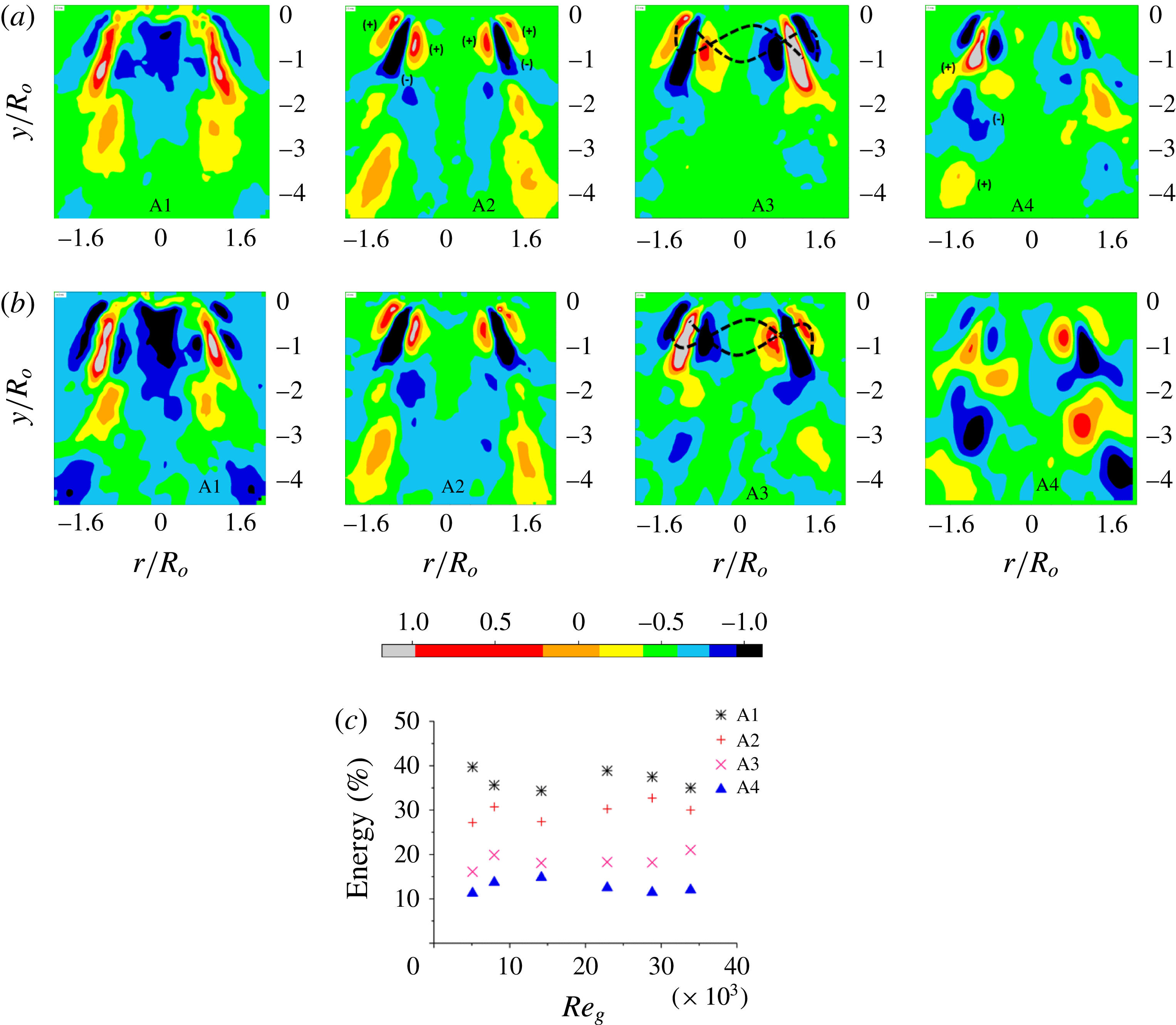
The spatial eigenmodes $\unicode[STIX]{x1D719}_{n}(x)$ pertaining to only the gas phase flow field (without droplets) are shown in figure 11. Here, only two flow conditions are shown for brevity, one for low airflow rate $(Re_{g}=5089)$ and the other for high airflow rate $(Re_{g}=33\,888).$ It should be noted that the eigenmodes depicted for both airflow rates look identical in the topological sense, due to the fixed value of the swirl number (as explained earlier in § 2). Logically, in POD, the number of eigenmodes is equal to the number of snapshots provided as input. However, only the first few modes contribute towards the overall TKE of the flow field. In the present experiments, the cumulative energy of first four modes (A1–A4) is found to be more than 95 % (see figure 11 c). Hence, only those eigenmodes are shown in figure 11(a,b).

Figure 11.

(a,b) Illustration of the POD spatial eigenmodes for only the gas phase for (a) $Re_{g}=5089$ and (b) $Re_{g}=33\,888$ . (c) The modal energy distribution. A1, first mode, KH instability/centrifugal instability; A2, second mode, KH instability/axial shear instability; A3, third mode, helical instability; A4, fourth mode, shedding mode. Adapted from Rajamanickam & Basu (Reference Rajamanickam and Basu2017).

Several studies (Billant et al. Reference Billant, Chomaz and Huerre1998; Gallaire & Chomaz Reference Gallaire and Chomaz2003) have reported the dominance of centrifugal or azimuthal shear instabilities in strongly swirling jets ( $S_{G}\geqslant 0.6$ ). The mechanism/type of the instabilities can be identified with the help of vorticity contours (spatial eigenmodes) and the frequency signatures (see figure 12) extracted from the temporal modes. From the viewpoint of the vorticity distribution along the longitudinal axis ( $y/r_{o}$ ), the instability waves can be delineated as symmetric or asymmetric. For instance, modes 1 and 2 exhibit symmetric vorticity distributions (figure 11 a,bA1,A2). Modes 3 and 4 exhibit asymmetric (i.e. helical; figure 11 a,bA3,A4) vorticity distributions.

The strong negative vorticity region observed in the central region of mode 1 (A1) is induced by VBB due to the intense rotation of the fluid in the azimuthal direction (i.e. strong swirling jet, $S_{G}\geqslant 0.6$ ). Moreover, in this region, the radial velocity magnitude shows dominance over the axial component $(\unicode[STIX]{x2202}U_{y}/\unicode[STIX]{x2202}r<\unicode[STIX]{x2202}U_{r}/\unicode[STIX]{x2202}y)$ . This results in a combination of axial and azimuthal shear.

Coles (Reference Coles1965) formulated the criteria for centrifugally unstable flows, which state that the flow becomes locally unstable if the vorticity magnitude in that region is negative (see (5.1)),

The dominance of azimuthal and axial shear in modes 1 and 2 is identified as the KH/strong shear instability mode. From the modal energy distribution viewpoint, it can be inferred that the flow field is dominated by azimuthal and axial shear instabilities (A1, A2) which account for 80 % of the total TKE. In contrast, modes 3 and 4 account for only 20 % of the energy.

In general, swirling jets exhibit helical waves before vortex breakdown occurs. This condition is true only for weak swirling jets (i.e. $S_{G}<0.6$ ). However, in this study, the flow condition pertains to a strong VBB state. Hence, the helical modes appear as low-energy-content modes ( ${\sim}$ 20 % of the total energy). It is important to note that the vorticity contours in the POD modes (in particular for A1, A2 and A3; figure 11 a,b) predominantly appear in the region where counter-rotating vortices are present, whereas only in the fourth mode (A4; low-energy-content mode) do the vortices appear in alternate fashion in the OSL region (figure 11 a,b,A4). The above observations clearly demonstrate the dominance of counter-rotating vortices over shedding vortices (only in the A4 mode). The origin of the shedding vortices in the swirl flow can be traced to the oscillations induced by the PVC (Syred Reference Syred2006; Martinelli, Olivani & Coghe Reference Martinelli, Olivani and Coghe2007).

Figure 12.

Illustration of frequency spectra obtained from the POD temporal modes for only the swirling gas flow field. Adapted from Rajamanickam & Basu (Reference Rajamanickam and Basu2017).

The frequency spectra obtained for modes 1 (A1) and 2 (A2) exhibit very narrow bands (see figure 12). The frequency values show an increasing trend with the flow rates from 30 Hz to 75 Hz for A1 and A2. However, repetitive frequency peaks are observed for the helical and shedding modes (A3, A4; figure 12). The important conclusion evident from the frequency signature is the nature of the instability wave induced in each mode. For instance, the single large peak observed around ${\sim}$ 75 Hz for A1 and A2 suggests long waves (i.e. the wavelength is relatively larger than those of modes 3 (A3) and 4 (A4) (i.e. $\unicode[STIX]{x1D706}_{1,2}>\unicode[STIX]{x1D706}_{3,4}$ )). Since, A1 and A2 are identified as KH instability modes, the frequency signature and wavelength scales pertaining to A1 and A2 are delineated as $f_{1,2}\approx f_{KH}$ and $\unicode[STIX]{x1D706}_{1,2}\approx \unicode[STIX]{x1D706}_{KH}$ respectively. Therefore, the frequency signatures in A1 and A2 are mainly contributed by large-scale coherence structures. On the other hand, small-scale/shedding eddies lead to the formation of multiple frequency peaks in A3 and A4. This may due to the coupling of large-scale coherent structures with low-energy-content eddies (i.e. small scale).

5.2 Spatial eigenmodes in the presence of droplets

The dominant instability mechanisms that govern the swirling flow field are presented in § 4.2. The objective of this section is to outline the qualitative and quantitative comparisons between the POD spatial eigenmodes pertaining to the flow field with and without droplets. The quantitative information involves coherence analysis between the temporal modes and the instantaneous spatially averaged circulation $\unicode[STIX]{x1D6E4}^{\prime }$ . This approach reveals the mechanisms behind the modal coupling between the two phases and the corresponding trends in the coherence function $C_{\unicode[STIX]{x1D6E4}^{\prime },\unicode[STIX]{x1D703}^{\prime }}(f)$ , as observed in figure 10. Since the main interest lies in identifying the instability mechanism involved during strong interaction, only flow rates corresponding to GL coupling $(Re_{g}\sim 33\,888,MR\sim 8164)$ are considered here for brevity.

Spatial eigenmodes evaluated from instantaneous vector fields involving droplets for two injection locations (OSL 1, 2; ISL 1, 2) are shown in figure 13. The modal contours pertaining to the flow field with droplets are marked as M1–M4. The contour maps of the spatial eigenmodes suggest strong coupling of the azimuthal shear modes (i.e. M1 and A1 shown in figures 11 and 13 are similar) for both OSL and ISL injections.

Figure 13.

The POD spatial eigenmodes computed from the instantaneous swirling gas flow field in the presence of droplets ( $MR\sim 8164$ ): (a) OSL 1; (b) OSL 2; (c) ISL 1; (d) ISL 2.

The fundamental difference observed in the eigenmodes between ISL and OSL injections is the appearance of secondary instability modes in the OSL case. For instance, mode 2 (M2) shown in figure 13(b) exhibits shedding as a secondary mode in addition to the shear mode (here, the shear mode is depicted inside the dotted black box) observed in the gas phase. The same observation is valid for M3 also, i.e. the appearance of a shedding mode in addition to the helical modes. In contrast, the ISL depicts only shear (i.e. azimuthal and axial shear) instabilities in the first two modes (see M1 and M2 in figure 13 c,d). The spatial eigenmodes quantified at downstream injection locations (OSL 3, ISL 3) also exhibit similar trends; hence, for brevity, these are shown in the supplementary material (figure S7i,ii).

It should be noted that in figure 12, the helical and shedding modes exhibit multiple frequency peaks. The coupling of secondary modes with highly energetic modes (i.e. M2) in the OSL is suspected to be a cause of the secondary frequencies $(f_{s})$ observed in the coherence analysis (figure 10 ai–iii). To confirm this phenomenon, coherence analysis is carried out between the temporal modes ( $a_{n}(t)$ ) and the forcing parameter $\unicode[STIX]{x1D6E4}^{\prime }$ :

Figure 14.

Coherence plots illustrating the dynamic coupling trends between the instantaneous circulation strength $\unicode[STIX]{x1D6E4}^{\prime }$ and the temporal modes $a_{n}(t)$ for $MR=8164$ : (a) OSL 1; (b) OSL 2; (c) OSL 3; (d) ISL 1; (e) ISL 2; (f) ISL 3.

The coherence analysis carried out as per (5.2) is graphically shown in figure 14. Again, the results are shown only for the strong-interaction (GL) case $(Re_{g}\sim 33\,888,MR\sim 8164)$ . For OSL injection (figure 14 a–c), it is seen that modes M1 and M2 become coupled with $\unicode[STIX]{x1D6E4}^{\prime }$ at very high coherence values of 0.8–0.9 in very narrow frequency band (90–110 Hz). In addition, mode 2 (M2, axial shear instability) shows intermediate coherence values of 0.3–0.5 at secondary frequency levels of 300–600 Hz. The interesting point to note in OSL injection is the activation of shedding modes (high-frequency modes) for downstream injection points in combination with high-energy-content modes, i.e. mode 2 (figure 14 b,c). This may be due to interaction of the droplets with shedding vortices (small-scale eddies). Moreover, the instantaneous raw images also suggest predominant interaction of droplets with these shedding vortices (see figure S8a and movie 4). Helical and shedding modes (M3 and M4) are coupled in higher and wider frequency bands (200–600 Hz) with lower coherence values. The existence of these secondary frequency bands was already established in the coherence analysis (§ 4) made between $\unicode[STIX]{x1D6E4}^{\prime }$ and $\unicode[STIX]{x1D703}^{\prime }$ (see figure 10 a).

On the contrary, in ISL injection, the droplets undergo breakup (see the blue dotted lines in figure S8b,c) before they reach the rotating eddies. This pre-breakup of droplets induces a drastic reduction in size, which ultimately leads to lower local Stokes number (see (7.5)) values. The lower Stokes number causes significant droplet trapping inside the vortex core, rather than the interaction with the shedding eddies as observed in the OSL. Modal coherence results for the ISL cases confirmed that the instantaneous circulation values $\unicode[STIX]{x1D6E4}^{\prime }$ are primarily coupled with only azimuthal and axial shear instability modes (M1 and M2; see figure 14 d–f), which results in high coherence values of 0.8–0.9 around 80–110 Hz. In both cases (OSL, ISL), the frequency spectra corresponding to KH instability modes are delineated as $(f_{KH})$ .

The coherence observations made in §§ 4 and 5 can be summarized as follows.

For the OSL,

For the ISL,

In summary, in this section, we found the mechanism behind the peculiar nature of coherence signatures corresponding to ISL and OSL injections.

6.1 High-speed visualization of vortex–droplet interaction

The flow conditions pertaining to two-way, transition and one-way interactions were identified in the global flow field characterization (§ 2). Instantaneous snapshots of droplet images corresponding to these interaction types are shown in figure 15(i),(ii). Interestingly, the interacting droplets exhibit several complicated structures (marked as red circles in figure 15i,iid–g) while breaking up into fragments. The driving mechanism for these breakups includes large-scale coherent structures present in the gas phase and the associated instability modes like KH shear and vortex shedding, as explained in the earlier sections.

6.2 Droplet breakup regimes

The droplets injected into vortices are subjected to oscillations induced by the swirling gas phase flow, leading to shape deformation and breakup. Several experimental and theoretical works (Hanson, Domich & Adams Reference Hanson, Domich and Adams1963; Simpkins & Bales Reference Simpkins and Bales1972) have been carried out to elucidate the droplet breakup mechanisms in coflowing air.

In general, the two major forces, namely the aerodynamic drag force $(F_{a})$ and the restoring surface tension force $(F_{\unicode[STIX]{x1D70E}})$ , involved in the droplet deformation/breakup process can be expressed in non-dimensional form (Weber number $We$ ) as follows:

The aerodynamic force induced by the vortex is given by

The detailed derivations and assumptions involved with (6.2) can be found in Oweis et al. (Reference Oweis, Van der Hout, Iyer, Tryggvason and Ceccio2005). Now, expression (6.2) can be rewritten as

Here, $\overline{\unicode[STIX]{x1D6E4}}$ is the time-averaged circulation strength, $\overline{r_{cc}}$ is the vortex core radius obtained from time-averaged flow field images, $\unicode[STIX]{x1D70E}$ is the interfacial tension and $D_{o}$ is the initial droplet diameter. In the present experiments, the initial injected droplets are predominantly monodispersed in nature with an average diameter of $500~\unicode[STIX]{x03BC}\text{m}$ . In addition, an instantaneous Weber number $(We^{\prime })$ is also proposed as a function of the instantaneous spatially averaged circulation strength $(\unicode[STIX]{x1D6E4}^{\prime })$ . Here, $We^{\prime }$ is evaluated from (6.3) except that $\unicode[STIX]{x1D6E4}^{\prime }$ is used instead of $\overline{\unicode[STIX]{x1D6E4}}$ .

Figure 16.

Illustration of breakup modes as a function of the time-averaged Weber number: (a) $(0<\overline{We}\leqslant 16,0<MR\leqslant 184)$ ; (b) $(16<\overline{We}\leqslant 57,184<MR\leqslant 450)$ ; (c) $(57<\overline{We}\leqslant 95,450<MR\leqslant 3720)$ ; (d) $(95<\overline{We}\leqslant 335,3720<MR\leqslant 5899)$ ; (e) $(335<\overline{We}\sim 500,5899<MR\leqslant 8164)$ .

It should be noted that $We^{\prime }$ and $\overline{We}$ are calculated in a small spatial window (at the location of first entry of droplets into the flow field, shown in figure S5) rather than around each droplet (which is impossible). The size of the spatial window (which varies with respect to the airflow rate; ${\sim}10\times 10{-}30\times 30~\text{mm}$ ) is chosen in such a way that the values of $\unicode[STIX]{x1D6E4}^{\prime }$ and $\overline{\unicode[STIX]{x1D6E4}}$ are largely insensitive to the box size so long it encompasses the high-vorticity region. Therefore, it is assumed that all droplets in that window experience the same circulation at any time instant. Hence, the Weber number is not based on individual droplets but rather on the initial diameter of the droplets entering the spatial window. In summary, $\overline{We}$ is a spatiotemporally averaged parameter, while $We^{\prime }$ is only a spatially averaged parameter evaluated at any given time instant.

For precise representation, the calculation of $We^{\prime }$ should involve the instantaneous droplet diameter and the local vortex strength $(\unicode[STIX]{x1D6E4}^{\prime })$ . However, this demands simultaneous measurement of individual droplet morphology (shape oscillations), tracking of droplet location and its surrounding flow field. This also requires a sufficiently lower number of droplets ( ${\sim}1~\text{droplet}~\text{s}^{-1}$ ) in the flow field. All of these are out of the scope of the current work.

In the present study, the droplet breakup can be viewed as two processes, primary and secondary. Primary breakup is the event that occurs where droplets first interact with eddies (mostly large scale) and yield fluid dynamically unstable structures like ligaments, non-spherical droplets, etc. (see the yellow circles in figure 16 c,d). These droplets may further undergo breakup (secondary) while interacting with the shedding eddies.

The various breakup modes observed as a function of the Weber number (6.3) are illustrated in figure 16. It should be noted that the breakup modes shown above do not pertain to any particular injection location. They are just sample illustrations of breakup mechanisms common across all injection locations as a function of the Weber number. However, the instantaneous interaction and dispersion mechanisms are found to be tightly coupled functions of the injection location, which will be illustrated in later sections. In common practice, droplet breakup is initiated if the Weber number $(\overline{We})$ exceeds a certain threshold/critical value $(\overline{We}_{c})$ . Theoretically, $\overline{We}_{c}$ is found to be ${\geqslant}$ 10 (Hinze Reference Hinze1955).

At this value, the waves formed over the droplet surface lead to multimodal shape oscillations (vibrational deformation), which ultimately result in breakup. In situations where lower aerodynamic forcing is involved, $0<\overline{We}<16$ , the surface tension damps the waves formed over the droplet surface, which mostly results in deformation/pinching of ligaments from the droplet surface (marked as red dotted lines in figure 16 a). In the current set-up, bag breakup ( $16<\overline{We}<57$ ; figure 16 b) occurs at a transitional Weber number (i.e. low airflow rate). The physical mechanism that governs this process is identified as differential pressure across the front and rear ends of the droplets (Han & Tryggvason Reference Han and Tryggvason1999).

Multimode breakup (figure 16 c) is witnessed for $450<MR\leqslant 1920$ . Dai & Faeth (Reference Dai and Faeth2001) categorized this breakup process as a transition between pressure difference induced bag and shear induced sheet thinning breakup modes. The different forms of breakup modes (vibrational, bag, multimode, sheet thinning, shear/catastrophic breakup) and their physical significance are elaborated in greater detail in Faeth et al. (Reference Faeth, Hsiang and Wu1995) and Guildenbecher et al. (Reference Guildenbecher, López-Rivera and Sojka2009). The governing mechanism involved with sheet thinning breakup (figure 16 d) is the formation of a boundary layer over the droplet surface due to the shear induced by fast moving gas (Nicholls & Ranger Reference Nicholls and Ranger1969; Chou, Hsiang & Faeth Reference Chou, Hsiang and Faeth1997). It involves deformation of the droplet periphery followed by stretching, formation of ligaments and subsequent breakup into daughter droplets. Catastrophic breakup (figure 16 e) is mostly encountered in extremely high-shear flows like the current swirling flow field (Hopfinger & Lasheras Reference Hopfinger and Lasheras1996). In this case, such breakup (figure 16 d,e) is mostly dominated by waves induced by surrounding gas phase instabilities (Taylor Reference Taylor and Batchelor1963; Hsiang & Faeth Reference Hsiang and Faeth1992). The resulting drop sizes in catastrophic breakup predominantly scale with the wavelength $\unicode[STIX]{x1D706}_{max}$ that exhibits the highest growth rate.

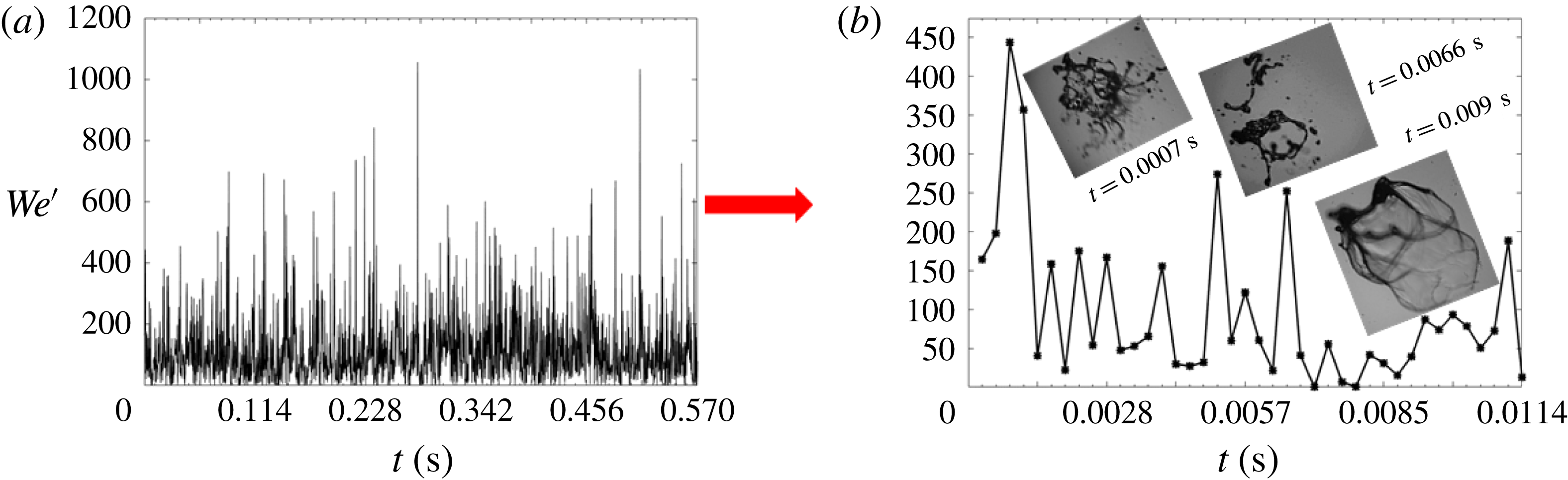
It is interesting to note that, even for a fixed gas flow rate, different breakup modes are witnessed. For instance, in figure 17(a,b), it is shown that the flow rate pertaining to $MR\sim 8164$ exhibits several breakup modes like bag, sheet thinning and catastrophic at different time instants. This is due to the fact that fluctuations in the instantaneous circulation (i.e. $\unicode[STIX]{x1D6E4}^{\prime }$ ) eventually lead to large-scale fluctuations in the instantaneous Weber number $We^{\prime }$ . This phenomenon is graphically illustrated in figure 17(b) for $MR\sim 8164$ over one cycle. Here, a cycle is considered based on a time scale $(\unicode[STIX]{x1D70F}=1/f_{KH})$ as calculated from the dominant frequency spectrum obtained from modal analysis (POD).

It can be observed (figure 17 a) that the instantaneous value of the Weber number shows a large variation ( ${\sim}$ 10–1050) during any one cycle of vortex shedding even though $\overline{We}$ is much lower ( ${\sim}$ 400). Hence, it is natural to witness a whole gamut of breakup modes consistent with such Weber number ranges. The average Weber number $(\overline{We})$ would fail to explain the detailed dynamics of droplet breakup in these flows.

Figure 17.

(a) Illustration of fluctuations observed in $We^{\prime }$ for a fixed flow rate ( $MR\sim 8164$ ). (b) Cyclic behaviour of the Weber number $(We^{\prime })$ for any given airflow rate ( $MR=8164$ ).

6.3 Analysis of droplet eigenmodes

To evaluate the modal coupling in the droplet breakup process, POD is implemented for instantaneous droplet images acquired from high-speed shadowgraphy. The procedure involved in computing the POD is the same as shown in figure S6. For brevity, only one injection position ( $y/R_{o}=1$ ) pertaining to OSL 1 and ISL 1 across three flow conditions ( $MR$ values) is shown. Similarly to the arguments made in coherence analysis, the eigenmodes (C1–C4) depict dominance of KH shear instability (i.e. mode 1, C1) in both cases. The results at the ISL suggest that even the second mode (C2) is shear dominant (figure 18 bii,iii). In contrast, the OSL exhibits shedding and shear as a combined mode. The other two modes (C3 and C4) are identified as helical and shedding modes. All of this modal information quantified from shadow images shows consistent behaviour, as seen in the flow field POD modes (figure 11). In coaxial atomization, it is well known that the atomization is driven by instability waves formed at the liquid–gas interface. The nature of the waves and their length scale $(\unicode[STIX]{x1D706}_{max})$ are solely determined by the source of perturbations (i.e. instabilities) involved in the breakup process. Studies (Liu, Mather & Reitz Reference Liu, Mather and Reitz1993; Chandrasekhar Reference Chandrasekhar2013) have identified that the wave growth over the droplet surface is predominantly described by Rayleigh–Taylor (RT) and KH instabilities.

Figure 18.

Spatial eigenmodes derived from high-speed instantaneous shadow images ( $MR=8164$ ): (a) OSL; (b) ISL; (i) OSL 1, ISL 1; (ii) OSL 2, ISL 2; (iii) OSL 3, ISL 3.

The KH mode is shown to be a prime cause, where droplets are subjected to large shear like vortices and jets in cross-flow, to name a few (Lasheras, Villermaux & Hopfinger Reference Lasheras, Villermaux and Hopfinger1998; Marmottant & Villermaux Reference Marmottant and Villermaux2004). Subsequently, secondary events like pinching of ligaments, their breakup and formation of daughter droplets are governed by the RT instability. Here, the qualitative information about the dominant wavelength $(\unicode[STIX]{x1D706}_{max})$ can be predicted from POD temporal mode frequency spectra. The most unstable wavelength $\unicode[STIX]{x1D706}_{max}$ and frequency $f$ are related as $f_{KH}\approx U_{i}/\unicode[STIX]{x1D706}_{max}$ , where $U_{i}$ is the interfacial velocity.

The frequency signatures derived using POD analysis for only the gas phase ( $A$ ) and for the combined liquid–gas phase ( $C$ ) are graphically shown in figure 19. Here, the results are presented as a function of the time-averaged Weber number $(\overline{We})$ . For low airflow rates $(\overline{We}<\overline{We}_{c})$ , the frequency signature between $A$ and $C$ exhibits a decoupling effect i.e. less dominance of gas phase instabilities (region I). It is to be noted that high frequency values are observed for the liquid phase ( ${\sim}800{-}1200~\text{Hz}$ ); this may be due to the small-scale disturbances imposed due to the dominance of the surface tension $\unicode[STIX]{x1D70E}$ (Squire Reference Squire1953; Marmottant & Villermaux Reference Marmottant and Villermaux2004). Beyond $\overline{We}\geqslant \overline{We}_{c}$ (i.e. region III), the dominance of the gas phase results in frequency values closer to the gas phase instability modes. In particular, the gas phase shear modes are completely synchronized with the droplet breakup process, $f_{A1,A2}\approx f_{C1,C2}$ . The lower magnitude of the frequency values observed in regions II and III is due to the long waves (Lasheras & Hopfinger Reference Lasheras and Hopfinger2000) induced by KH instabilities $(\unicode[STIX]{x1D706}_{max}\sim \unicode[STIX]{x1D706}_{KH})$ present in the swirling gas flow field.

In the KH dominated wave region, the speed of propagation of the interface/shear layer ( $U_{i}$ ) induced by the most dominant wave can be related to the Dimotakis speed (Cebeci & Bradshaw Reference Cebeci and Bradshaw1977; Dimotakis Reference Dimotakis1986).

Figure 19.

Modal frequency signature comparison between the swirling gas phase flow field ( $A$ ) and the high-speed instantaneous shadow images ( $C$ ) of the droplets.

The theoretical expression involves balance of dynamic pressure of the two fluid streams (liquid and gas phases) across the shear layer,

where $\overline{V_{d}}$ and $\overline{V_{\unicode[STIX]{x1D714}}}$ are the time-averaged velocities of the droplets and vortices; $\overline{V_{\unicode[STIX]{x1D714}}}=\overline{\unicode[STIX]{x1D6E4}}/2\unicode[STIX]{x03C0}r$ . This condition will hold true only when the gas phase is extremely turbulent and the liquid flow is laminar ( $\overline{V_{\unicode[STIX]{x1D714}}}\gg \overline{V_{d}}$ or $V_{i}>\overline{V_{d}}$ ). The time scale $(\unicode[STIX]{x1D70F}=1/f_{KH})$ pertaining to a cyclic event of the two-phase interaction observed from high-speed shadow images suggests an inline behaviour with Dimotakis speed (6.5). This implies that the acceleration of the interface is predominantly governed by KH waves.

In summary, the primary breakup process is mostly dominated by counter-rotating vortices rather than shedding vortices. However, the shedding vortices may contribute towards further breakup of ligaments/droplets pinched off from the initial droplets during the primary interaction.

The corresponding $MR$ values for the aforementioned time-averaged Weber number regimes (I, II, III) are as follows:

1. (I) $\overline{We}<\overline{We}_{c}\rightarrow 0\leqslant MR<450$ , two-way GL–LG regime (movie 6);

2. (II) $\overline{We}\approx \overline{We}_{c}\rightarrow 450<MR\leqslant 1920$ , transition to one-way G–L regime (movie 7);

3. (III) $\overline{We}\geqslant \overline{We}_{c}\rightarrow 3720\leqslant MR\leqslant 8164$ , strong one-way GL regime (movie 8).

7.1 Global dispersion field

The global dispersion field is computed by tracking the individual particles/droplets present in the instantaneous flow field images (acquired with simultaneous PIV). The technique used here computes the spatial location of each droplet present in a given frame (the steps are shown in figure S9). With the computed spatial information $(r/R_{o}^{\prime },y/R_{o})$ on the droplets, a time-averaged dispersion map (see figure 20 a,b and figure S10a,b) is generated for the three Weber number regimes (I, II, III) as shown in figure 19. In figure 20, only two representative cases pertaining to OSL and ISL are shown, the remaining cases can be found in the supplementary material (see figure S10).

From figure 20(a,b), it is perceived that for low Weber numbers, $\overline{We}<\overline{We}_{c}$ , the droplets are not widely dispersed because of low momentum transfer from the gas phase. In this regime (I, II), the breakup process (vibrational, bag) does not yield any smaller sized droplets, which in turn causes the Stokes number to be very high ( $St\gg 1$ ). The quantitative treatment of the Stokes number ( $St$ ) will be elucidated in the size distribution section (see the supplementary material, § 2.5). This ( $St\gg 1$ ) prevents the droplets from dispersing effectively in the flow field. The same mechanism is observed for both OSL and ISL injections. On the contrary, in regime III, the breakup process dominated by gas phase shear instabilities yields several smaller sized droplets (see figure 16 c–e). Among these smaller sized droplets, those satisfying $St\ll 1$ follow the gas flow path effectively.

Figure 20.

The spatial dispersion of the droplets across the three flow regimes (I, II, III): (a) OSL 1; (b) ISL 1 ( $MR=0$ , 450, 8164).

(i) Dispersion mechanism in the OSL. In § 5, it is inferred that even for one particular flow rate, fluctuations in $\unicode[STIX]{x1D6E4}^{\prime }$ lead to different breakup mechanisms (bag, multimode, catastrophic). In this context, two major forms of dispersion field are observed in the OSL. First, when $\unicode[STIX]{x1D6E4}^{\prime }<\unicode[STIX]{x1D6E4}_{c}^{\prime }$ , the injected droplets predominantly do not interact with the vortices and rather penetrate inside the vortex core (figure 21 ai). In this situation, the droplets are mostly subjected to axial shear, which results in either bag or multimode breakup. This induces very few smaller sized droplets of Stokes number $St<1$ , which are entrained in the recirculation region ( $0.5\leqslant r/R_{o}\leqslant -0.5$ ; see figure 21 ai). On the other hand, when $\unicode[STIX]{x1D6E4}^{\prime }>\unicode[STIX]{x1D6E4}_{c}^{\prime }$ , on account of strong interaction with vortices, the droplets undergo catastrophic breakup, which yields a greater number of small-sized droplets. Subsequent to breakup, only the $St\gg 1$ droplets stay in the OSL region ( $-0.6\leqslant r/R_{o}\leqslant 1.6$ ; see figure 21 aii) due to the resistance offered by high-strength vortices. Moreover, the droplets in these regions tend to disperse radially outwards due to the transfer of gas phase swirl momentum to the droplets. The small-sized droplets ( $St<1$ ) are entrained in the recirculation region; few droplets of $St\sim 1$ are found to penetrate inside.

Figure 21.

The qualitative dispersion mechanisms of the injected droplets in the swirling gas flow field as a function of the Stokes number ( $St$ ),  $MR=8164$ : (a) OSL 1; (b) ISL 1.

(ii) Dispersion mechanism in the ISL. The fundamental difference observed in the dispersion among the ISL and OSL injections is the formation of droplet clusters within the VCC in the ISL region (shown as dotted circles in figures 20 b and S10b). Further, here the droplets are first deflected upwards from the point of injection before they interact with the vortices. In the ISL, as already elucidated in the global flow field section, the vortex strength is not disturbed by injected droplets. This implies that at high airflow rates, the droplets in the ISL are predominantly subjected to shear breakup, which ultimately leads to much smaller droplet sizes. The droplets with Stokes numbers of order $O(\ll 1)$ are trapped inside the recirculation zone (see figure 21 b). Further downstream of the VCC, the droplets with $St<1$ are entrained by recirculated flow (indicated as a blue line in figure 21 b). In addition to the spatial clustering observed with counter-rotating eddies, the shedding eddies contribute to droplet cluster formation (particularly for downstream injections $y/R_{o}=1$ , 1.5 in figure S10b). The remaining droplets $(St\gg 1)$ stay in the outside region $(-2\leqslant r/R_{o}\leqslant -3)$ . This clustering of droplets with large-scale eddies creates spatial non-uniformity in the dispersion process. This phenomenon can be viewed as a result of inertial clustering due to the response between the carrier phase and the dispersed phase (Fessler, Kulick & Eaton Reference Fessler, Kulick and Eaton1994; Kulick et al. Reference Kulick, Fessler and Eaton1994).

In addition, the more qualitative nature of the droplet dispersion/response with respect to the swirling gas flow field can be understood from the flow field induced by the droplets. To do this, vector postprocessing is implemented on PIV raw images considering only droplets in the flow field (i.e. without seeding the gas flow). It is well known that in PIV, the flow field can be delineated only if the injected particle response has a linear relationship with the flow time scale (Raffel et al. Reference Raffel, Willert, Wereley and Kompenhans2013). The vector field reconstructed by considering only droplets in the flow field is shown in the supplementary material (see figure S11) for brevity.

The qualitative view of the spatial dispersion of the droplets in the swirling gas phase flow field is presented in § 7, where the global picture is elucidated as a function of the Stokes number. The more quantitative information in terms of the size distribution is presented in supplementary § 2.5 (figure S12). In figure S12, the droplet size distribution pertaining to region III (i.e. $\overline{We}>\overline{We}_{c}$ ) is subdivided into three regimes in terms of the Stokes number (figure S12b,c). For higher $We$ ( $We>500$ ), the diameter distribution shows polydisperse characteristics in two predominant ranges of ${\sim}10{-}20~\unicode[STIX]{x03BC}\text{m}$ ( $St<1$ ; see figure S12b,c) and ${\sim}50{-}60~\unicode[STIX]{x03BC}\text{m}$ ( $St>1$ ) for both ISL and OSL injections. The droplet size corresponding to $St<1$ is identified as the critical diameter ( $D_{critical}$ ). It should be noted that ISL injection exhibits a greater number of $St\ll 1$ droplets than OSL injection (see figure S12b,c).

8.1 Dispersion-governing parameters

The instantaneous droplet dispersion and spatial homogeneity may exhibit higher or lower values than the ones shown here in the time-averaged map. The major parameter that governs this process is the local/global Stokes number, which in turn is a function of the fluctuations in the vortex strength induced by gas phase instabilities and the cyclic behaviour of the Weber number in the temporal domain, as already illustrated in figure 17.

Figure 22.

Illustration of the spatial inhomogeneity of the droplet dispersion in the swirling gas flow field: (a) OSL; (b) ISL.

In addition, other variables like droplet–droplet and droplet–gas velocity correlations and turbulence modulations are also shown to be parameters responsible for the spatial dispersion (Mashayek Reference Mashayek1998; Balachandar & Eaton Reference Balachandar and Eaton2010; Sahu, Hardalupas & Taylor Reference Sahu, Hardalupas and Taylor2014). These effects are not explicitly considered in this study.

In § 4, it is shown that any perturbation applied to $\unicode[STIX]{x1D6E4}^{\prime }$ is reflected in the droplet response $\unicode[STIX]{x1D703}^{\prime }$ . In a given set of time series images, the droplet responses may vary (i.e. phase). For instance, the cyclic behaviour of the Weber number shown in figure 17 exhibits orderly repetitiveness over the time period (see figure 23 a). To illustrate this phenomenon, the phase-averaged dispersion angle $\overline{\unicode[STIX]{x1D703}}_{\emptyset }=\sum _{i=1}^{n}(((\unicode[STIX]{x1D703}_{\emptyset }^{\prime })_{1}+\cdots +(\unicode[STIX]{x1D703}_{\emptyset }^{\prime })_{n})/N)$ is evaluated from the given set of time series images (see figure 23). The dispersion angle corresponding to the peak value observed in each cycle is considered as instantaneous, $\unicode[STIX]{x1D703}_{\emptyset }^{\prime }$ . The steps involved in the calculation of $\overline{\unicode[STIX]{x1D703}}_{\emptyset }$ are shown in figure 23(a). The graph suggests that the phase-averaged dispersion angle $\overline{\unicode[STIX]{x1D703}}_{\emptyset }$ differs by a factor of ${\sim}10^{\circ }{-}15^{\circ }$ in GL interaction regimes (III) compared with the time-averaged dispersion angle $\overline{\unicode[STIX]{x1D703}}$ . Another influencing parameter is the choice of spatial injection location. Again, both axial and radial positions yield considerable change in the dispersion field. The dispersion of the droplets injected in the near field $(y/R_{o}\leqslant 1;\text{OSL }1,2;\text{ISL }1,2)$ is predominantly governed by counter-rotating eddies. On the other hand, the shedding vortices play a significant role in the case of droplets injected at downstream positions $(y/R_{o}>1;\text{OSL }3;\text{ISL }3)$ .

Figure 23.

(a) The steps involved in extraction of the phase-averaged dispersion angle $(\overline{\unicode[STIX]{x1D703}}_{\emptyset })$ are shown over three cycles. (b,c) Comparison of the time-averaged droplet response $(\overline{\unicode[STIX]{x1D703}})$ with the phase-averaged $(\overline{\unicode[STIX]{x1D703}}_{\emptyset })$ response for (b) OSL 2 and (c) ISL 2.