

Introduction
Understanding the underlying drivers of species richness has been a primary focus for conservation and ecology. Nationally and globally, prioritization efforts have designated areas of rare habitats with high numbers of endemic species as regions on which to focus conservation resources (Jenkins et al. Reference Jenkins, Pimm and Joppa2013). However, wildlife surveys often occur at smaller geographic scales and require conservationists to merge information from broad, general strategies with local metrics of animal occupancy. In such cases, conservation efforts that support species richness across regional areas can be problematic because research has not yet determined the optimal area to associate local-level animal monitoring data with remotely sensed habitat metrics (i.e., scale; sensu Jackson & Fahrig Reference Jackson and Fahrig2012). Conservationists need to better understand how important coarse-scale habitat metrics correlate with species richness at fine scales and to translate regional conservation measures into local action.
Remote sensors are beneficial in performing repeated standardized measurements over a range of spatial scales (He et al. Reference He, Bradley, Cord, Rocchini, Tuanmu and Schmidtlein2015). The information from these sensors provides great potential to investigate relationships between vertebrate richness and habitat metrics at both fine and coarse scales across landscapes (Davies & Asner Reference Davies and Asner2014). These products are also essential tools for tracking progress towards biodiversity and conservation goals, such as the Aichi Biodiversity Targets, utilizing metrics of primary productivity, fragmentation and fire regimes (Secades et al. Reference Secades, O’Connor, Brown and Walpole2014). What has not garnered sufficient attention in the development of these metrics is that the shape of the relationships between the remotely sensed and ground-based data varies with scale (Tews et al. Reference Tews, Brose, Grimm, Tielbörger, Wichmann, Schwager and Jeltsch2004).
The core issue is that factors important at coarse scales do not always translate well to fine scales and vice versa. Environmental measures at coarse scales tend to homogenize landscapes into the dominant habitat or land-cover type, but do not detect important factors for fine-scale habitat selection (Boyce Reference Boyce2006). For example, coarse-scale productivity and habitat heterogeneity metrics based on the normalized difference vegetation index are positive indicators of avian diversity, but are negatively associated with avian diversity at fine scales within temperate forests (Bae et al. Reference Bae, Müller, Lee, Vierling, Vogeler, Vierling and Hudak2018). This is true for other vertebrate taxa as well. Important coefficients for elk habitat selection change in magnitude, and even direction, with increasing measurement scale (Boyce et al. Reference Boyce, Mao, Merrill, Fortin, Monica, Fryxell and Turchin2003). Unfortunately, coarse-scale environmental data (e.g., 1 km2) used to test species–environmental relationships tend to break down to non-significant relationships at finer scales in c. 60% of vertebrate richness studies (Mittelbach et al. Reference Mittelbach, Steiner, Scheiner, Gross, Reynolds and Waide2001). Conversely, fine-resolution environmental data (e.g., 1 m2) must be summarized to a scale that is appropriate for application. To better inform conservation we need to link animal point surveys to fine-resolution remote sensing data amalgamated at broader scales, correcting for the spatial extent at which remotely sensed covariates are most highly correlated with species occupancy and, to a further extent, species richness (Jackson & Fahrig Reference Jackson and Fahrig2012).
The difficulty in matching remote sensing data with animal detections may be related to the various scales at which animals utilize their habitats. Johnson (Reference Johnson1980) described a hierarchical order of selection dependent on the scale of habitat use and availability. The coarse scale of selection (first-order selection) is the distribution of a species across large areas; second-order selection is the home range of an individual within the larger landscape; third-order selection is habitat patches within an individual’s home range; and fourth-order selection is for resources within these patches. Coarse-scale measures of environmental data smooth important localized heterogeneity and productivity gradients, while measurements at fine scales only sample habitats relative to fourth-order selection (Tews et al. Reference Tews, Brose, Grimm, Tielbörger, Wichmann, Schwager and Jeltsch2004). The optimal match between remote-sensing data and local-level animal measures may depend on the scale at which animals truly select habitats, in which case the most appropriate scale will vary between vertebrate taxonomic groups based on resource and home range requirements (Wiens Reference Wiens1989).
In this study, we tested the influence of habitat heterogeneity and productivity on species richness using a range of local measurement scales to determine whether optimal scales exist when modelling species richness. Both LiDAR and hyperspectral imagery were used to measure habitat heterogeneity and productivity across a local landscape in northern Virginia (c. 1800 ha). Our goal was, first, to identify the scaling effects associated with modelling species richness and, second, to identify optimal scales at which remotely sensed measures of habitat heterogeneity and productivity best predict ground-based measures of vertebrate richness. We predicted that the richness of each taxonomic group would be better estimated using measurement scales approximating the average home-range sizes determined by life history and resource needs. The results of this study increase our understanding of scaling issues that arise when modelling species richness using habitat metrics and identify appropriate scales for using fine-resolution remote-sensing data.
Methods
Survey sites
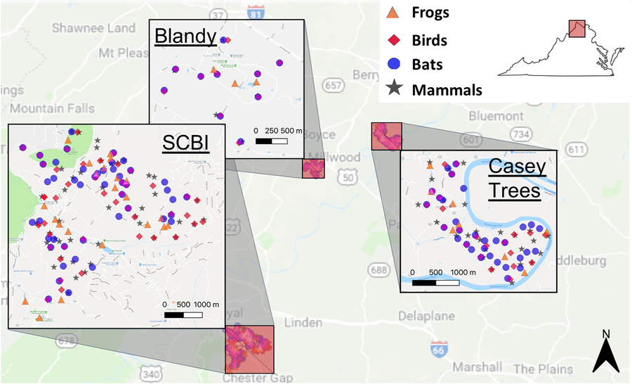
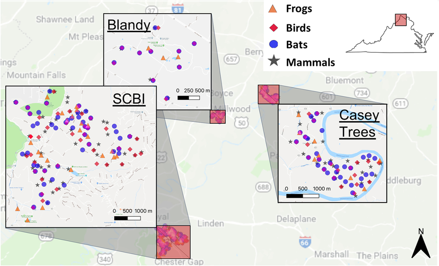
Research took place at three northern Virginia sites, the Smithsonian Conservation Biology Institute (38°53′18.38″N, 78°09′52.38″W), Blandy Experimental Farm (39°03′48.72″N, 78°03′46.84″W) and Casey Tree Farm (39°05′25.60″N, 77°58′36.92″W), which represent a gradient of management intensity (Fig. 1). We selected these sites as part of the National Earth Observatory Network (NEON; Domain 2) and used a randomized grid algorithm to select sample locations (Reversed Randomized Quadrant-Recursive Raster; Theobald et al. Reference Theobald, Stevens, White, Urquhart, Olsen and Norman2007). We used the National Land Cover Database 2011 to create forest and open habitat classifications, defining ‘forest’ by the combination of forest, woody wetlands and shrub/scrub habitat classes and ‘open’ by the combination of cultivated and grassland/herbaceous habitat classes (Homer et al. Reference Homer, Dewitz, Yang, Jin, Danielson and Xian2015).
The three study sites and all camera trap and acoustic recording unit locations in northern Virginia. Targeted survey locations are represented by unique symbols indicating each surveyed group: frogs (triangles), birds (diamonds), bats (circles) and mammals (stars). SCBI = Smithsonian Conservation Biology Institute.
Monitoring methods
We selected survey locations for each vertebrate taxon based on habitat requirements. Frog species were sampled within 10 m of a constant water source. Bat survey locations were selected from four categories: (1) open areas; (2) within 5 m of a road or forest edge; (3) within 20 m of a water source within a forest; and (4) within a forest at least 60 m from a road or a water source. Birds and terrestrial mammals were surveyed within areas classified as ‘open’ or ‘forested’. All survey points were separated by at least 200 m.
Wildlife Acoustics’ SM3BAT acoustic recording units (ARUs) surveyed bird, bat and frog richness. ARUs were sampled with 16-bit digitization and a 24-kHz sample rate for birds and frogs and a 256-kHz sample rate for bats. ARUs were attached directly to trees c. 2 m above ground level with an acoustic microphone connected directly to the unit when surveying for frogs and birds (Depraetere et al. Reference Depraetere, Pavoine, Jiguet, Gasc, Duvail and Sueur2012). For bats, we elevated an ultrasonic microphone 4.5 m above the ground to increase signal detection in the canopy.
We matched the diel and seasonal timing of ARU deployment to the peak activity for each group: bats were surveyed from sunset to sunrise during July and August (Skalak et al. Reference Skalak, Sherwin and Brigham2012); birds were surveyed for 3 hours starting 30 minutes before sunrise from late May through June (Wimmer et al. Reference Wimmer, Towsey, Roe and Williamson2013); and frogs were surveyed for 3 hours starting 30 minutes before sunset and again for 3 hours starting 30 minutes before sunrise from March through May (De Solla et al. Reference De Solla, Shirose, Fernie, Barrett, Brousseau and Bishop2005). During each survey period for frogs and birds, the ARU recorded 1 minute out of every 10 minutes. When sampling bats, the ARUs only recorded when triggered by ultrasonic frequencies (>8 kHz) that reached a threshold of 12 decibels for a duration of 3–15 seconds. Each ARU deployment lasted 3 weeks for frogs and 1 week for birds and bats. Both birds and frogs were surveyed with two deployments at each location coinciding with the early and late breeding season.
We surveyed the terrestrial mammal community with camera traps (Reconyx PC-800). We placed cameras c. 50 cm in height with commercial carnivore scent lure (Pro’s Choice) applied to a small object 3 m in front of the unit. Each camera was deployed for 3 weeks to accurately detect mammal occupancy within this region (McShea et al. Reference McShea, Forrester, Costello, He and Kays2016). Camera deployments began in April and ended in August to coincide with the time of year in which these mammals are most active.
Data processing
We reduced processing time by eliminating any file without peak frequencies above 1 kHz using the seewave package in R version 3.3.2 (R Development Core Team 2010; Sueur et al. Reference Sueur, Pavoine, Hamerlynck and Duvail2008). From the remaining files, experts identified all frog species. For birds, we further identified the peak time of acoustic diversity using soundecology (Villanueva-Rivera & Pijanowski Reference Villanueva-Rivera and Pijanowski2018) and identified the first 1.5-hours of daily recordings (30 minutes before sunrise to 1 hour after sunrise) for further analysis. Birds were then identified from a random subsample of 50 1-minute recordings from each site within this 1.5-hour period.
We used Kaleidoscope Pro (version 3.1.4B) to estimate nightly occupancy for bats. We specified the filter setting at a minimum of three pulses between 12 and 120 kHz and between 2 and 500 ms. The software estimated nightly occupancy probabilities for each species based on the strength of identifications and the known misclassification rates found by Britzke et al. (Reference Britzke, Murray, Heywood, Robbins, Kurta and Kennedy2002). Kaleidoscope utilized a maximum-likelihood estimator approach to determine species presence at a site. Post hoc maximum-likelihood estimator p-values were used to determine final occupancy with a threshold of 0.05. These probabilities were then verified with spectrograms and converted into binary data for use in our occupancy models.
After retrieving each camera trap, we processed and managed the photographs and metadata using the eMammal web application (www.emammal.si.edu). Species in each triggered photograph sequence, as defined by Forrester et al. (Reference Forrester, O’Brien, Fegraus, Jansen, Palmer, Kays and Ahumada2016), were manually identified. This information was then approved by an expert in a second review process. The photographs and metadata were then stored in the eMammal repository.
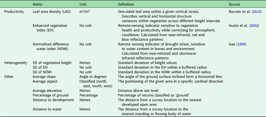
We derived habitat heterogeneity and productivity metrics from NEON’s Airborne Observation Platform, which flew over these sites in August 2016 (Supplementary Table S1, available online; see Table 1 for a full list of metrics) (NEON, 2017b). The platform included a full-waveform LiDAR sensor and a hyperspectral imaging spectrometer. We standardized the classified LiDAR point-cloud before calculating metrics using the lidR package (Roussel & Auty Reference Roussel and Auty2018). LiDAR measurements included leaf area density (LAD) as a three-dimensional measure of productivity in the form of vegetation density (Kamoske et al. Reference Kamoske, Dahlin, Stark and Serbin2019) and the percentage of first returns classified as ‘ground’ as an estimate of gaps within the vegetation. In addition to these habitat measurements, we calculated slope, aspect and elevation. Hyperspectral metrics included the enhanced vegetation index (EVI) and normalized difference water index (NDWI). We calculated the mean EVI and NDWI for each location using the raster package (Hijmans Reference Hijmans2017).
A list of all metrics used during this study, including their units and definitions. Measures fall into one of three categories labelled in the left-most column, including productivity, heterogeneity and other factors.

We averaged scale-dependent measurements over buffered areas ranging from a 20-m radius to a 180-m radius for birds, bats and frogs and up to 220 m for terrestrial mammals with 20-m increments centred on each survey location. We did not consider scales less than 20 m due to the risk of erroneous environmental measures when using LiDAR metrics such as LAD, which begin to provide stable results at scales of 10 m and larger (Kamoske et al. Reference Kamoske, Dahlin, Stark and Serbin2019). We did not analyse scales large than 220 m because our results indicated decreasing performance after 180 m for terrestrial mammals, and there were no indications that these correlations constituted a bimodal process. For each measurement scale, we scaled and centred each metric on zero across survey locations.
Occupancy covariates included remote sensing measurements of productivity, heterogeneity and other explanatory factors. Productivity included undergrowth LAD (0–3 m), aboveground LAD (for frogs and mammals; >3 m), understory LAD (for birds and bats; 3–15 m), mid-canopy LAD (for birds and bats; 15–30 m), upper-canopy LAD (for birds and bats; >30 m), EVI and NDWI. Heterogeneity measures included the standard deviation in EVI and NDWI (horizontal heterogeneity) and the standard deviation in vegetation height (vertical heterogeneity). Other occupancy covariates included average slope, aspect and elevation to account for local variance in species richness.
Detection covariates varied with daily survey periods and included mean daily temperatures, mean daily wind speeds and total daily precipitation. Daily weather measurements were taken by NEON at each site on a 30-minute basis (Supplementary Table S1) (NEON, 2017a). The LAD at the height of the ARU (0–3 m for birds and 3–15 m for bats) was also used as a detection covariate, as obstruction of vegetation around the acoustic devices can limit detections.
We assessed spatial independence with a Moran’s I test using the coordinates of each survey location and the observed species richness at neighbouring survey locations. Moran’s I p-values and correlation values were obtained using the R package lctools (Kalogirou Reference Kalogirou2017) with an α value of 0.05 considered significant.
To consider functional groups within each taxon, we organized species into guilds, with distinct assemblages of species linked by shared habitat needs, foraging behaviours and body size. Mammals were split into two guilds based on diet (omnivore or herbivore) and two guilds based on body size (small ≤5 kg; large >5 kg). Bats were divided in two guilds, including species with high-frequency calls (≥40 kHz) and species with low-frequency calls (<40 kHz). Avian species were classed into three separate guild configurations based on habitat, foraging and nesting behaviour (Rodewald Reference Rodewald2015). Habitat classifications included forest, grassland and edge guilds. Foraging classifications included aerial, bark, foliage and ground guilds. Nesting classifications included cavity nests, cup nests in trees and cup nests in shrubs guilds. There were insufficient natural history data to group frogs into guilds.
To compare optimal scales to home-range size, we considered the home-range sizes of select species within each group as examples of the larger group. A common frog species, the wood frog (Lithobates sylvaticus), has a home range sizes of 0.08 ha (Blomquist & Hunter Reference Blomquist and Hunter2010). Songbirds such as the common red-eyed vireo (Vireo olivaceus) and the rarer cerulean warbler (Setophaga cerulea) have breeding home ranges of between 0.4 and 0.7 ha, respectively (Barg et al. Reference Barg, Aiama, Jones and Robertson2006, Marshall & Cooper Reference Marshall and Cooper2004). Big brown bats (Eptesicus fuscus) have documented home ranges of up to 2900 ha in size (5 km from their roost); however, these bats used distinct foraging areas more intensively within this range (Menzel et al. Reference Menzel, Carter, Jablonowski, Mitchell, Menzel and Chapman2001). For larger mammals, the mean home range can vary drastically. Larger predators like the coyote (Canis latrans) have a home range of 7600 ha (Ozoga & Harger Reference Ozoga and Harger1966), while smaller mammals, such as the eastern grey squirrel (Sciurus carolinensis), have significantly smaller home range sizes of c. 1 ha in size (Flyger Reference Flyger1960).
Statistical analysis
We used a two-step hierarchical Bayesian approach to evaluate the optimal scale for each vertebrate group. First, we used a pair of multi-species Bayesian occupancy models at each scale (Dorazio et al. Reference Dorazio, Royle, Söderström and Glimskär2006). One model was used to generate true occupancy for individual species using occupancy data from all sites, and a second model was used to predict species-specific occupancy for a set of validation sites where observed data were withheld from the model (c. 30% of the survey locations). Second, we calculated area under the receiver operating characteristic curve (AUC) in a Bayesian framework from the posterior distribution of predicted occupancy with each iteration (Zipkin et al. Reference Zipkin, Grant and Fagan2012). We then used these AUC values for a quantitative comparison of predictive performance at each scale.
We fitted our models using the jags function in the package R2jags version 0.5–0.7 (Su & Yajima Reference Su and Yajima2015; see sample code for our model in Supplementary Appendix S1). For all models, we ran three Markov chains of length 8000 with a burn-in of 3000 iterations and 1/4 thinning. Convergence was indicated with an R-hat value of less than 1.1 (Gelman & Hill Reference Gelman and Hill2006). We used posterior predictive checks to ensure that the final models were predicting values consistent with the data as a measure of model fit (Supplementary Table S2). AUC values for each iteration of the models were calculated with the R package ROCR version 1.0–7.0 (Sing et al. Reference Sing, Sander, Beerenwinkel and Lengauer2005). The 95% credible intervals (CI) of these estimates were then calculated using the R package BEST version 0.5.1 (Kruschke & Meredith Reference Kruschke and Meredith2018). We considered the guild grouping with the highest mean AUC scores on average as the most appropriate for our discussion. The most appropriate scale was considered to be the model with the maximum mean AUC value and non-overlapping CI.
Results
Survey results
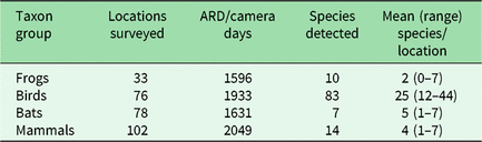
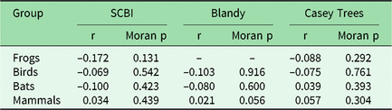
Our ARU and camera trap arrays were able to sample species’ presence data from 204 unique locations across the three sites, including 33 frog, 76 bird, 78 bat and 102 terrestrial mammal survey locations (Table 2). We have provided full species lists and accompanying numbers of observations for frogs (Supplementary Table S3), bats (Supplementary Table S4), birds (Supplementary Table S5) and terrestrial mammals (Supplementary Table S6) as supplementary information. Moran’s I test results suggested no significant spatial autocorrelation between species richness and the proximity of survey locations (Table 3).
Summary of acoustic recording device (ARD) and camera trap surveys with apparent species detected. The survey effort is summarized across survey sites as the number of days (for frogs, birds and mammals) or the number of nights (for bats).

Results of Moran’s I tests for spatial autocorrelation at each site for each target vertebrate group. Resulting p-values indicate that no significant relationship exists between species observed and the distance between sites.

‘–’ indicates too few sites sampled for testing.
SCBI = Smithsonian Conservation Biology Institute.
Scale and performance
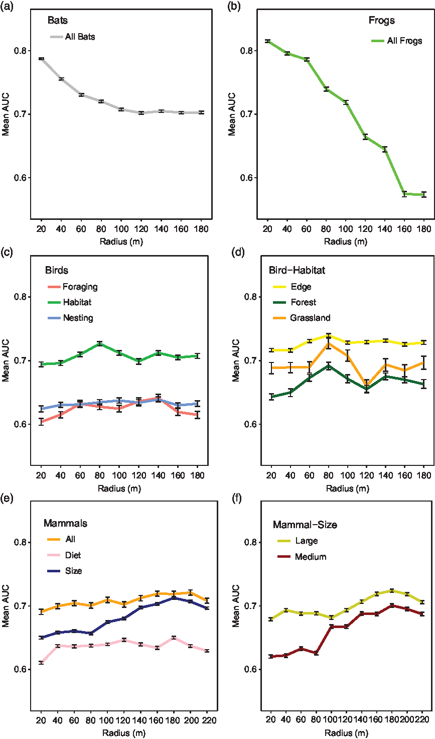
The performance of the frog and bat multi-species occupancy models varied widely depending on the measurement scale. The maximum mean AUC values for both frog and bat models indicated a spatial scale with a 20-m radius with no overlap in AUC CI at other scales. The resulting maximum mean AUC values for models at the optimal scale were 0.81 (CI = 0.81–0.82) for frogs and 0.79 (CI = 0.78–0.79) for bats (Fig. 2(a) & 2(b)). The optimal scale was approximately the same size as the home range of the wood frog, but the optimal scale for bats was significantly smaller than the home range of the big brown bat.
A summary table of area under the receiver operating characteristic curve (AUC) prediction scores at each scale tested for (a) bats, (b) frogs, (c & d) birds and (e & f) terrestrial mammals. Each point represents the mean AUC values with error bars indicating 95% credible intervals averaged for all groups and guilds.
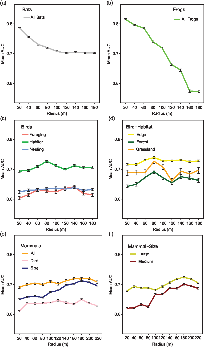
For birds, the model performance varied depending on both scale and guild. The mean AUC values were highest for the habitat guilds with a maximum mean AUC = 0.73 using an 80-m radius (CI = 0.72–0.73) (Fig. 2(c)). For the forest birds, the maximum mean AUC value resulted in a mean AUC value of 0.69 (CI = 0.69–0.70) (Fig. 2(d)). For the grassland birds, the optimal spatial scale resulted in a mean AUC of 0.73 (CI = 0.72–0.74) (Fig. 2(d)). For the edge species, the optimal spatial scale resulted in a mean AUC of 0.74 (CI = 0.73–0.74) (Fig. 2(d)). For these three habitat guilds, there was no overlap in the AUC CI at other scales. The mean AUC values of models ran with both the foraging (range: 0.60–0.64) and nest (range: 0.62–0.64) guilds were much lower than those of models for habitat guilds (Fig. 2(c)). The models associated with nesting and foraging classifications were dropped from further analysis due to their lower performance compared to the habitat models. The resulting optimal scale at 80 m was similar to the home range size of the two songbirds considered for comparison.
Terrestrial mammal model performance varied depending on both the measurement scale and the guild. There was no difference between the AUC results of 160-m, 180-m and 200-m measurement scales when modelling all species together (Fig. 2(e)). However, there were differences between these scales when modelling terrestrial mammal guilds based on body size and diet type. However, model selection for both large and small body-sized mammals resulted in maximum mean AUC values with a 180-m radius and mean AUC scores of 0.72 (CI = 0.72–0.73) and 0.70 (CI = 0.69–0.70), respectively, with no overlap in credible intervals at other scales (Fig. 2(f)). This optimal scale is significantly smaller than the home range of the coyote, but this scale is much larger than the home range of the eastern grey squirrel. The diet guilds performed worse than body-sized guilds (Fig. 2(e)) and were dropped from further analysis in this study.
Differences of scale
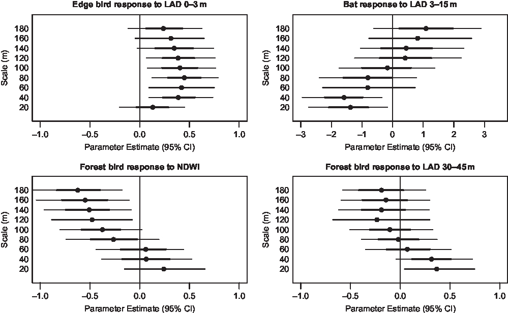
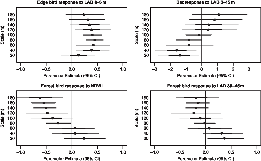
We investigated the strength and relationship of all model parameters at each scale. Many of these parameters were scale dependent, changing in magnitude and direction with increasing scale of measure. For example, when estimating bird species richness, LAD in the upper canopy resulted in a positive relationship, not overlapping zero with 20-m scaled measurements. However, as the measurement scale increased, the strength of this parameter was steadily reduced to zero with 80-m scaled measurements and shifted to a negative relationship at coarser scales. Another example resulted from estimating edge bird richness with a 20-m scaled measure of understory LAD. At this scale the parameter was not important, overlapping zero, but the relationship became significantly positive as the scale was increased to 80 m, and then decreasing in strength as the measurement scale increased towards 180 m. Many other covariates share this wavering trend between positive, neutral or negative relationships as the scale of measure is increased (Fig. 3).
Representative graphs of mean bat, edge bird and forest bird community parameters in terms of specific productivity and heterogeneity covariates across scales. Thick error bars indicate 50% credible intervals (CI) and thin error bars indicate 95% CI. LAD = leaf area density; NDWI = normalized difference water index.
Discussion
Using remote-sensing data to approximate species richness obtained by point surveys of animals is the primary means by which international metrics of vertebrate biodiversity will be measured (Proença et al. Reference Proença, Martin, Pereira, Fernandez, McRae and Belnap2017). Estimates of species richness rely on accurate species occurrences within a given area of interest. Matching point surveys to fine-scale habitat metrics are possible. However, we demonstrate that differences do exist in the strength and relationship of habitat metrics across a range of scales to accurately predict species occupancy, which is ultimately used for estimates of species richness. We identify optimal scales for local habitat heterogeneity and productivity metrics when predicting species richness, but the best scale is not always equivalent to the average home-range size of the species we considered as examples for each group.
For birds, the results from this study demonstrate that relatively small changes in scale are important considerations when modelling the relationships between the avian community and metrics of habitat heterogeneity and productivity. For example, avian forest species are positively associated with productivity covariates such as NDWI or LAD at smaller scales (20–60-m buffer areas), but the parameters associated with these measures shift to negative associations at coarser scales. Alternatively, other measures (i.e., upper-canopy LAD) shift towards negligible effect sizes with increasing scale for estimating forest guild richness. When using the 80-m optimal scale, forest birds were negatively related to NDWI and the effect of upper-canopy LAD was negligible, but if we had not evaluated a range of scales and only used a 20-m buffer, we would have come to opposite conclusions.
Similarly, measurement scale is an important consideration for modelling bat species richness. Community correlations shifted from positive to negative relationships and vice versa as the measurement scale increased. The strongest correlation observed indicates that richness is negatively related to increased vegetation density (LAD) from 3 to 15 m within the optimal 20-m buffer. However, if a coarser scale is used, bat richness results in a positive relationship with this metric. We know that bats can have large home-range sizes, such as the big brown bat mentioned earlier; thus, it is possible that coarser scales would perform better (i.e., >200-m buffer). However, if these scales were relevant, we would expect an increasing AUC score with scale, which is not the trend observed. One possible explanation for the importance of fine-scale metrics is habitat use, where some species occupy ‘beats’ within 100 m of roost sites for foraging once they have established a home range (Senior et al. Reference Senior, Butlin and Altringham2005). For bats, like birds, the scale at which the habitat is measured becomes critical for understanding the relationships between habitat variables and species richness.
Unlike for birds and bats, community relationships for frog species remain fairly consistent for each covariate regardless of scale. However, the overall negative trend in model performance with increasing measurement scale indicates that the parameter estimates at finer scales best represent frog occupancy for multiple species. The steep drop in model performance with scale suggests that high-resolution metrics should be used for modelling amphibians, since coarser remote-sensing metrics will likely miss the strength of these localized relationships.
In comparison, measurement scales are less influential for the terrestrial mammal community, as indicated by the weaker performance and small differences in AUC values between scales. This could be due in part to the larger differences in home-range size compared to other taxonomic groups. We acknowledge that we are not able to adequately test our hypothesis with terrestrial mammals, specifically larger mammals, because of large differences in home-range size between individual species, but we include this group in comparison to the results of other taxonomic groups. We were limited in our capacity to model scales larger than the home-range size for several of our mammal species, and thus a 220-m scale should not be considered an endpoint. It is possible that scales used in single-species occupancy models could correspond better with home-range size; however, the purpose of this study was to see whether optimal scales exist for different taxonomic groups in relation to species richness, and if so, how these scales relate back to the average home range of the group considered. We strongly recommend future studies with larger study areas in order to explore larger scales and investigate how these relationships might differ between individual species as well.
Optimal scales are important because measurements that are too coarse have led to incorrect assumptions and conclusions (McGarigal et al. Reference McGarigal, Wan, Zeller, Timm and Cushman2016). By using multiple taxonomic groups for this study, we show that home range may not always be the best indicator of optimal measurement scale. Drawing inferences from Johnson’s (Reference Johnson1980) framework, we find that the optimal scale of habitat heterogeneity and productivity metrics is equivalent to areas of second- and third-order habitat selection for a range of vertebrate taxa. Habitat metrics for taxonomic groups that utilize the entirety of their home range to satisfy life history requirements, such as birds and frogs, are best linked to second-order selection scales. Alternatively, habitat measures used for taxonomic groups that utilize specific areas more intensively, such as terrestrial mammals and bats, are better linked to third-order selection scales.
Conclusion
There is not a consistent optimal scale across taxonomic groups for linking common habitat metrics to estimates of species richness. General patterns show that scales equivalent to home-range size are better indicators of occupancy and richness for taxonomic groups regularly utilizing the entirety of their home range. For taxonomic groups that divide their home range into distinct areas of activity, the best scale may reflect the size of the foraging areas within a home range. Remotely sensed heterogeneity and productivity measures to predict species richness vary in power among functional taxonomic groups and are sensitive to issues of scale. Therefore, the same habitat measurement scale cannot be used to model all vertebrate taxa and should be carefully considered when setting conservation metrics across local or regional areas. These results should serve as a step towards scaling up new information to conservation metrics at regional or national levels.
Supplementary material
To view supplementary material for this article, please visit https://doi.org/10.1017/S0376892919000328.
Acknowledgements
Our group is indebted to the support and resources provided by the Smithsonian Conservation Biology Institute (SCBI), George Mason University (GMU) and the National Science Foundation (NSF). We thank Blandy Experimental Farm and Casey Tree Nursery for allowing us to use their property for surveys and the National Ecological Observation Network (NEON) for allowing us to pair survey sites with their ongoing research and for sharing survey designs and protocols. We also thank Joel Mota and Sarah Macey for their hard work and determination during fieldwork and recording analysis.
Financial support
This work was supported by a grant from the National Science Foundation (NSF) EAGER #1450318 and NSF Division of Emerging Frontiers award number EF #1823498, as well as the Smithsonian Conservation Biology Institute and George Mason University.
Conflict of interest
None.
Ethical standards
The authors assert that all procedures contributing to this work comply with applicable ethical standards relevant to Section 7009 of the America Creating Opportunities to Meaningfully Promote Excellence in Technology, Education, and Science Act implemented by the National Science Foundation as responsible conduct of research.