



1. Introduction
Buoyancy-driven natural-convection boundary layers on heated surfaces control heat exchange between solid boundaries and quiescent fluids, with their spatial structure and temporal evolution setting local and global heat-transfer rates (Gebhart et al. Reference Gebhart, Jaluria, Mahajan and Sammakia1988; Bejan Reference Bejan2013). Classical understanding has been developed largely for canonical geometries subject to isothermal or uniform-heat-flux conditions (Ostrach Reference Ostrach1988). Many practical configurations, however, involve curved surfaces exposed to circumferentially non-uniform heating, for which geometric curvature and spatially varying thermal forcing jointly determine the local buoyancy field. Examples include solar-receiver tubes in concentrating solar power systems, where irradiation is concentrated on one side of the tube while the opposite side is weakly heated (Rodríguez-Sánchez et al. Reference Rodríguez-Sánchez, Soria-Verdugo, Almendros-Ibáñez, Acosta-Iborra and Santana2014; Logie et al. Reference Logie, Pye and Coventry2018), and horizontal cryogenic propellant tanks in launch vehicles and hydrogen-fuelled aircraft, where solar irradiation and aerodynamic heating can generate circumferential temperature gradients (Verstraete et al. Reference Verstraete, Hendrick, Pilidis and Ramsden2010). Related configurations also occur in geophysical and environmental settings, including ice shelves and frozen pipes immersed in stratified ambients (Kerr & McConnochie Reference Kerr and McConnochie2015). Despite their prevalence, it remains an open question how the angular variation imposed by surface curvature interacts with that imposed by non-uniform wall temperature to shape both the transient growth and the steady boundary-layer state.
Because buoyancy is aligned with the principal flow direction, vertical-wall configurations have served as the canonical setting for the theory of natural-convection boundary layers. Analytical and similarity methods first characterised the steady laminar structure (Ostrach Reference Ostrach1952; Sparrow & Gregg Reference Sparrow and Gregg1956), followed by stability analyses of the leading-edge-generated disturbances on the developing boundary layer (Armfield & Patterson Reference Armfield and Patterson1992; Ke et al. Reference Ke, Williamson, Armfield, McBain and Norris2019) and simulations of the additional unsteady routes induced by cavity confinement (Xu et al. Reference Xu, Patterson and Lei2009b ; Gao et al. Reference Gao, Podvin, Sergent, Xin and Chergui2018). Scaling analysis, in particular, has extracted the essential parameter dependencies without full resolution of the governing equations: following Patterson & Imberger (Reference Patterson and Imberger1980), subsequent work quantified the Prandtl-number dependence and the role of thermal diffusion in the initiation of the flow under both isothermal (Lin et al. Reference Lin, Armfield and Patterson2007, Reference Lin, Armfield, Patterson and Lei2009; Lin & Armfield Reference Lin and Armfield2012) and isoflux (Armfield et al. Reference Armfield, Patterson and Lin2007; Lin et al. Reference Lin, Armfield and Patterson2008; Lin & Armfield Reference Lin and Armfield2020) conditions. Experiments have complemented these efforts, resolving the distinct transient stages (Patterson et al. Reference Patterson, Graham, Schöpf and Armfield2002; Xu et al. Reference Xu, Patterson and Lei2005) and the three-dimensional transition structures on vertical walls (Zhao et al. Reference Zhao, Lei and Patterson2015).
Spatial variation of the thermal forcing on vertical walls has also been studied. Sparrow & Gregg (Reference Sparrow and Gregg1958) showed that similarity solutions exist only for particular wall-temperature distributions, such as power-law or exponential forms, so that arbitrary variations preclude a classical similarity reduction. Scaling analysis has since been extended to linearly varying wall temperature on a semi-infinite plate (Liu Reference Liu2019), to a cooled sidewall driving an intrusion front in an open cavity (Liu Reference Liu2020) and to a linearly non-uniform heat flux (Liu & Zhu Reference Liu and Zhu2023), together spanning a broad range of Prandtl numbers. Further departures from uniform conditions include convective wall heating (Nie & Xu Reference Nie and Xu2019), time-dependent wall temperature (Lin & Armfield Reference Lin and Armfield2017) and heat flux (Lin & Armfield Reference Lin and Armfield2013) and non-instantaneous initiation (Patterson et al. Reference Patterson, Lei, Armfield and Lin2009), while in enclosed geometries spatially periodic heating can trigger instabilities that remain subcritical under uniform heating (Hossain & Floryan Reference Hossain and Floryan2013) and, combined with topography or slot inclination, generate net flows (Abtahi & Floryan Reference Abtahi and Floryan2017; Floryan et al. Reference Floryan, Baayoun, Panday and Bassom2022a , Reference Floryan, Wang, Panday and Bassomb ). These studies are, however, largely confined to flat walls or planar slots, leaving the interaction between non-uniform heating and surface curvature unresolved.
Natural convection on horizontal cylinders differs fundamentally from the vertical-wall case because the tangential component of buoyancy varies with azimuthal position. For a uniformly heated cylinder, this component scales as
 $g\beta (T_w-T_\infty )\sin \theta$
, driving an accelerating boundary layer from the lower stagnation point, with progressive thickening and eventual detachment into a buoyant plume near the upper pole. Here,
 $g$
is the magnitude of gravitational acceleration and
 $\beta$
is the thermal expansion coefficient.
 $T$
denotes temperature, with
 $T_w$
and
 $T_{\infty}$
representing the cylinder-wall and ambient-fluid temperatures, respectively. The angular coordinate
 $\theta$
is measured anticlockwise from the lower stagnation point. The steady structure of this boundary layer has been analysed using series-expansion and integral methods (Merk & Prins Reference Merk and Prins1953, Reference Merk and Prins1954; Merkin Reference Merkin1977), and the associated global heat-transfer rates have been incorporated into widely used Nusselt-number correlations (Churchill & Chu Reference Churchill and Chu1975; Morgan Reference Morgan1975). Recently, scaling analysis has been extended to the transient development of natural-convection boundary layers on heated horizontal cylinders under both isothermal and isoflux conditions, over a wide range of Prandtl numbers (Liu & Ren Reference Liu and Ren2021; Liu & Ma Reference Liu and Ma2024; Ma & Liu Reference Ma and Liu2024). In these studies, however, the wall temperature or heat flux is spatially uniform. In practical configurations, non-uniform thermal conditions arise naturally from circumferential variations in external heating, contact resistance or conjugate conduction effects, making spatially varying wall temperature a more representative boundary condition. When the wall temperature varies with angular position, the buoyancy field contains two coupled sources of angular dependence: the geometric
 $\sin \theta$
modulation intrinsic to the cylinder and the imposed circumferential variation of the thermal forcing. This coupling may alter the circumferential self-similarity that underpins existing scaling laws and Nusselt-number correlations, yet it has not been addressed systematically and forms the central problem of this study. The linear wall-temperature distribution adopted here is an idealised first-order representation of the smooth circumferential temperature gradients that may arise under one-sided or biased external heating, while retaining a single parameter that isolates the effect of thermal non-uniformity.
Motivated by this unresolved coupling, our study explores the transient natural-convection boundary layer on a horizontal cylinder whose wall temperature varies linearly with azimuthal position under Boussinesq conditions. A scaling analysis, validated against the present numerical simulations, is developed for the full evolution from the initial transient stage to the steady state. The initial regime is governed by diffusion-dominated growth and remains locally controlled, whereas the steady regime requires an energy-integral formulation that accounts for the cumulative influence of upstream buoyancy forcing. This distinction provides a unified framework for describing boundary-layer development under circumferentially non-uniform heating and for identifying when local buoyancy scaling fails. The resulting predictions are tested over the numerical dataset. The physical model and numerical method are presented in § 2. The initial and steady-stage scaling analyses are developed in §§ 3 and 4, respectively. The broader implications and limitations of the results are discussed in § 5, and the main findings are summarised in § 6.
Physical model and wall-temperature condition: (a) horizontal cylinder, coordinate system and boundary-layer structure; (b) dimensionless wall-temperature distributions for different values of the wall-temperature-gradient parameter
 $s$
, with fixed equatorial and mean wall-to-ambient temperature difference
 $\Delta T_0$
.

Figure 1. Long description
Panel A: A schematic diagram of a horizontal cylinder with a coordinate system and boundary-layer structure. The diagram shows a cylinder with radius R, surrounded by a boundary layer with thickness delta_T(θ) and delta_v(θ). The coordinate system includes radial (u_r) and angular (u_θ) velocity components, and the angle θ varies from 0 to π. The wall temperature T_w(θ) is indicated, with ambient temperature T∞ and pressure p∞ outside the boundary layer. Gravity g acts downward. Panel B: A line graph depicting dimensionless wall-temperature distributions for different values of the wall-temperature-gradient parameter s. The x-axis represents the dimensionless temperature difference (T_w(θ) - T∞)/ΔT0, and the y-axis represents the angle θ/π. The graph includes multiple lines for different values of s (0.0, 0.5, 1.0, 1.5, 2.0), showing how the wall temperature varies with the angle for each parameter value. The constant mean temperature line is also shown.
2. Problem formulation
2.1. Physical model and governing equations
We consider transient natural convection from a heated horizontal circular cylinder of diameter
 $D=0.4$
m and radius
 $R=D/2$
immersed in an initially quiescent, isothermal fluid. The cylinder is assumed to be sufficiently long such that end effects are negligible and the flow may be treated as two-dimensional. A polar-coordinate system
 $(r,\theta )$
is adopted with its origin at the cylinder centre, as shown in figure 1(a). The angular coordinate
 $\theta$
is measured from the lower stagnation point,
 $\theta =0$
, and increases anticlockwise towards the upper stagnation point,
 $\theta =\pi$
.
For
 $t\lt 0$
, the cylinder and the surrounding fluid are at rest and in thermal equilibrium at the ambient temperature
 $T_\infty$
. At
 $t=0$
, the cylinder surface is impulsively brought to a prescribed circumferentially non-uniform temperature distribution
 $T_w(\theta )$
, specified below. The fluid is Newtonian and incompressible, with constant kinematic viscosity
 $\nu$
and thermal diffusivity
 $\alpha$
. Density variations are retained only in the buoyancy term through the Boussinesq approximation (Gray & Giorgini Reference Gray and Giorgini1976; Patterson & Imberger Reference Patterson and Imberger1980; Ahlers et al. Reference Ahlers, Brown, Fontenele Araujo, Funfschilling, Grossmann and Lohse2006),
 $\rho \approx \rho _\infty [1-\beta (T-T_\infty )]$
, where
 $\rho _\infty$
is the reference density at
 $T_\infty$
and
 $\beta$
is the thermal expansion coefficient. Viscous dissipation and radiative heat transfer are neglected.
Gravity acts vertically downward,
 $\boldsymbol{g}=-g\hat {\boldsymbol{e}}_z$
. With
 $\theta$
measured from the bottom of the cylinder, its projections onto the polar basis are
 $ g_r=-g\cos \theta$
, and
 $g_\theta =g\sin \theta$
, where
 $g_r$
is positive in the outward radial direction and
 $g_\theta$
is positive in the direction of increasing
 $\theta$
. The buoyancy acceleration under the Boussinesq approximation is therefore
 $g\beta (T-T_\infty )(-\cos \theta \,\hat {\boldsymbol{e}}_r+\sin \theta \,\hat {\boldsymbol{e}}_\theta )$
. Thus the tangential component of buoyancy, proportional to
 $(T-T_\infty )\sin \theta$
, drives the boundary-layer motion along the cylinder surface, while the radial component is balanced primarily by the pressure field in the thin-layer limit.
To remove the hydrostatic contribution associated with the quiescent reference state, the total pressure is decomposed as
 \begin{align} p_{{total}} = p_s + p, \quad \boldsymbol{\nabla }\!{p}_s = \rho _\infty \boldsymbol{g}, \end{align}
where
 $p_s$
is the hydrostatic pressure for a fluid of uniform density
 $\rho _\infty$
, and
 $p$
is the perturbation pressure. Substitution of (2.1) together with the Boussinesq approximation into the Navier–Stokes equations eliminates the hydrostatic balance from the momentum equation. The resulting formulation is therefore written in terms of
 $p$
, with the departure of the density from
 $\rho _\infty$
appearing only through the buoyancy force.
Under these assumptions, the governing equations (Kuehn & Goldstein Reference Kuehn and Goldstein1980; Gebhart et al. Reference Gebhart, Jaluria, Mahajan and Sammakia1988; Bejan Reference Bejan2013) are written in terms of the perturbation pressure
 $p$
as
 \begin{align} \boldsymbol{\nabla }\boldsymbol{\cdot }\boldsymbol{u} &= 0,\end{align}
 \begin{align} \frac {\partial \boldsymbol{u}}{\partial t} + \boldsymbol{u}\boldsymbol{\cdot }\boldsymbol{\nabla }\boldsymbol{u} &= -\frac {1}{\rho _\infty }\boldsymbol{\nabla }\!{p} + \nu {\nabla} ^2 \boldsymbol{u} + g\beta (T-T_\infty ) \left ( -\cos \theta \,\hat {\boldsymbol{e}}_r + \sin \theta \,\hat {\boldsymbol{e}}_\theta \right ),\end{align}
 \begin{align} \frac {\partial T}{\partial t} + \boldsymbol{u}\boldsymbol{\cdot }\boldsymbol{\nabla }T &= \alpha {\nabla} ^2 T .\end{align}
Here,
 $\boldsymbol{u}=u_r\hat {\boldsymbol{e}}_r+u_\theta \hat {\boldsymbol{e}}_\theta$
is the velocity field and
 $p$
is the perturbation pressure introduced in (2.1). The expanded polar-coordinate form of (2.2)–(2.4) is given in Appendix A. In the scaling analysis below, the component form is used only to identify the dominant balances and the leading curvature contributions. In particular, the tangential component of (2.3) contains the buoyancy term
 $g\beta (T-T_\infty )\sin \theta$
, which drives the boundary-layer motion along the cylinder surface. This term couples the local thermal field to the geometric projection factor
 $\sin \theta$
, which vanishes at the lower and upper stagnation points and reaches its maximum geometric value at the equator. When the wall temperature also varies with
 $\theta$
, this geometric modulation is coupled to an imposed thermal modulation, distinguishing the present configuration from the uniformly heated cylinder.
The initial and boundary conditions are
 \begin{align} & t\lt 0\colon && \boldsymbol{u}=\boldsymbol{0}, && T=T_\infty && \text{for } r \geq R, \\[-12pt] \nonumber \end{align}
 \begin{align} & t\geq 0\colon && \boldsymbol{u}=\boldsymbol{0}, && T=T_w(\theta ) && \text{at } r=R, \\[-12pt] \nonumber \end{align}
 \begin{align} & && \boldsymbol{u}\to \boldsymbol{0}, && T\to T_\infty && \text{as } r\to \infty . \\[10pt] \nonumber \end{align}
The imposed wall temperature is symmetric about the vertical plane passing through the lower and upper stagnation points. The solution therefore satisfies left–right symmetry along
 $\theta =0$
and
 $\theta =\pi$
, where
 \begin{align} \frac {\partial u_r}{\partial \theta }=0, \quad u_\theta =0, \quad \frac {\partial T}{\partial \theta }=0 \quad \text{at } \theta =0,\pi . \end{align}
To isolate the effect of circumferential thermal non-uniformity from changes in the overall heating level, the wall temperature is prescribed as the simplest one-parameter departure from uniform heating that preserves the mean wall-to-ambient temperature difference. The linear distribution allows
 $s=0$
to recover uniform heating, while increasing
 $s$
systematically varies the circumferential temperature gradient. The distribution is written as
 \begin{align} T_w(\theta )=T_\infty +\Delta T_0 \left [ 1+s\left (\frac {\theta }{\pi }-\frac {1}{2}\right ) \right ]\!, \end{align}
where
 $\Delta T_0=T_w(\pi /2)-T_\infty$
is the reference temperature difference at the equator and is kept fixed for all values of
 $s$
. The dimensionless parameter
 $s$
measures the imposed circumferential temperature gradient
 \begin{align} s=\frac {\pi R}{\Delta T_0} \frac {\mathrm{d}T_w}{\mathrm{d}(R\theta )} =\frac {\pi R S}{\Delta T_0}, \end{align}
where
 $S=\mathrm{d}T_w/\mathrm{d}(R\theta )$
is the constant dimensional gradient along the arc length. A property of this linear form is that the mean wall-to-ambient temperature difference over
 $0\leq \theta \leq \pi$
 \begin{align} \frac {1}{\pi }\int _0^\pi [T_w(\theta )-T_\infty ]\,\mathrm{d}\theta = \Delta T_0 , \end{align}
is independent of
 $s$
. As shown in figure 1(b),
 $s=0$
recovers the uniformly heated cylinder,
 $T_w=T_\infty +\Delta T_0$
, whereas
 $s=2$
gives the largest monotonic stratification considered here, with
 $T_w(0)=T_\infty$
at the lower stagnation point and
 $T_w(\pi )=T_\infty +2\Delta T_0$
at the upper stagnation point. Values
 $s\gt 2$
would make
 $T_w\lt T_\infty$
near the lower stagnation point and locally reverse the sign of buoyancy. The present study therefore restricts attention to
 $0\leq s\leq 2$
, for which the wall-to-ambient temperature excess remains non-negative everywhere.
The local wall-to-ambient temperature difference is
 \begin{align} \Delta T(\theta )\equiv T_w(\theta )-T_\infty = \Delta T_0 \left [ 1+s\left (\frac {\theta }{\pi }-\frac {1}{2}\right ) \right ]\!. \end{align}
Combined with the geometric projection factor
 $\sin \theta$
, this temperature difference produces a tangential driving acceleration proportional to
 $\Delta T(\theta )\sin \theta$
. The problem, therefore, contains two coupled angular dependences: one imposed by the wall temperature and one imposed by the cylinder geometry.
The equations are non-dimensionalised using the cylinder diameter
 $D$
as the length scale, the velocity scale
 $U_0=\alpha Ra^{1/2}/D$
, the time scale
 $D/U_0=D^2/(\alpha Ra^{1/2})$
, the pressure scale
 $\rho _\infty U_0^2$
and the temperature scale
 $\Delta T_0$
. The velocity scale follows from the classical transient natural-convection balance between buoyancy and thermal diffusion (Patterson & Imberger Reference Patterson and Imberger1980; Lin et al. Reference Lin, Armfield and Patterson2007, Reference Lin, Armfield, Patterson and Lei2009; Liu Reference Liu2019). Introducing
 \begin{align} \boldsymbol{x}^*=\frac {\boldsymbol{x}}{D}, \quad \tau =\frac {t}{D/U_0}, \quad \boldsymbol{u}^*=\frac {\boldsymbol{u}}{U_0}, \quad p^*=\frac {p}{\rho _\infty U_0^2}, \quad \phi =\frac {T-T_\infty }{\Delta T_0}, \end{align}
and omitting asterisks hereafter, the dimensionless governing equations become
 \begin{align} \boldsymbol{\nabla }\boldsymbol{\cdot }\boldsymbol{u} &= 0, \\[-12pt] \nonumber \end{align}
 \begin{align} \frac {\partial \boldsymbol{u}}{\partial \tau } + \boldsymbol{u}\boldsymbol{\cdot }\boldsymbol{\nabla }\boldsymbol{u} &= -\boldsymbol{\nabla }\!{p} + \frac {Pr}{Ra^{1/2}}{\nabla} ^2\boldsymbol{u} + Pr\,\phi \left ( -\cos \theta \,\hat {\boldsymbol{e}}_r + \sin \theta \,\hat {\boldsymbol{e}}_\theta \right )\!, \\[-12pt] \nonumber \end{align}
 \begin{align} \frac {\partial \phi }{\partial \tau } + \boldsymbol{u}\boldsymbol{\cdot }\boldsymbol{\nabla }\phi &= \frac {1}{Ra^{1/2}}{\nabla} ^2 \phi . \\[10pt] \nonumber \end{align}
The dimensionless time is related to the Fourier number by
 $\tau =Fo\,Ra^{1/2}$
, where
 $ \textit{Fo}=\alpha t/D^2$
. The governing dimensionless groups are the Rayleigh and Prandtl numbers,
 \begin{align} Ra=\frac {g\beta \Delta T_0 D^3}{\nu \alpha }, \quad Pr=\frac {\nu }{\alpha }, \end{align}
along with the non-uniformity parameter
 $s$
defined in (2.10). The corresponding dimensionless wall temperature is
 \begin{align} \phi _w(\theta )=1+s\left (\frac {\theta }{\pi }-\frac {1}{2}\right )\!. \end{align}
Here,
 $ \textit{Ra}$
ranges from
 $10^6$
to
 $10^8$
,
 $ \textit{Pr}$
from
 $2$
to
 $100$
and
 $s$
from
 $0$
to
 $2$
. Since
 $ \textit{Pr}\gt 1$
throughout the parameter space, the thermal boundary layer is thinner than the velocity boundary layer, consistent with classical laminar natural-convection scaling. The largest Rayleigh number considered is
 $ \textit{Ra}=10^8$
. Previous studies of natural convection from horizontal cylinders report laminar boundary layers over this range (Rath & Dash Reference Rath and Dash2020), while simulations of related transient natural-convection boundary layers remain laminar beyond it (Lin & Armfield Reference Lin and Armfield1999; Xu et al. Reference Xu, Patterson and Lei2010). Consistent with these studies, the present computations show no persistent temporal oscillations, symmetry breaking or secondary flow structures after the transient adjustment. The results therefore characterise the laminar scaling regime of the two-dimensional problem. The complete set of governing parameters is summarised in table 1.
Non-dimensional parameter space for the simulations. Each
 $ \textit{Ra}$
is combined with all listed values of
 $ \textit{Pr}$
and
 $s$
, giving 120 cases. The Prandtl numbers are representative of common working fluids:
 $ \textit{Pr}=2$
and
 $7$
of hot and room-temperature water,
 $ \textit{Pr}=20$
of organic solvents such as alcohols and
 $ \textit{Pr}=50$
–
 $100$
of glycols, silicone oils and light lubricating oils.

Table 1. Long description
A table summarizing non-dimensional parameter space for simulations. The table has four columns and four data rows. Column headers are Case, Ra, Pr, and s. Row 1: Case 1-30, Ra 1 times 10 to the power of 6, Pr 2, 7, 20, 50, 70, 100, s 0, 0.5, 1.0, 1.5, 2.0. Row 2: Case 31-60, Ra 1 times 10 to the power of 7, Pr 2, 7, 20, 50, 70, 100, s 0, 0.5, 1.0, 1.5, 2.0. Row 3: Case 61-90, Ra 5 times 10 to the power of 7, Pr 2, 7, 20, 50, 70, 100, s 0, 0.5, 1.0, 1.5, 2.0. Row 4: Case 91-120, Ra 1 times 10 to the power of 8, Pr 2, 7, 20, 50, 70, 100, s 0, 0.5, 1.0, 1.5, 2.0.
The dimensional governing equations are solved by direct numerical simulation using a finite-volume method on a structured grid. Pressure–velocity coupling is handled with the semi-implicit method for pressure-linked equations pressure-correction procedure. Convective fluxes are discretised using the quadratic upwind interpolation for convective kinematics scheme for the momentum equations and a second-order upwind scheme for the energy equation, and time advancement is performed with a second-order implicit method. This numerical approach follows methods previously validated for natural-convection boundary layers (Xu et al. Reference Xu, Patterson and Lei2009a ; Nie & Xu Reference Nie and Xu2022; Jiang et al. Reference Jiang, Zhao, Carmeliet, Nie and Xu2024; Ma & Liu Reference Ma and Liu2025).
The computational domain is an annulus extending from the cylinder surface,
 $r=R$
, to an outer boundary at
 $R_\infty =10D$
. The far-field condition in (2.7) is imposed at
 $r=R_\infty$
using a pressure-outlet condition with zero normal velocity gradient; any inflow through this boundary is prescribed at the ambient temperature
 $T_\infty$
. Domain-size tests with
 $R_\infty =5D$
and
 $20D$
confirmed that the results are insensitive to the outer-boundary location. The domain is discretised using an O-type grid with
 $N_r\times N_\theta =360\times 600$
nodes. The radial spacing expands geometrically from the wall with a stretching ratio of
 $1.005$
, and the first-cell height satisfies
 $\Delta r_{\textit{min}}/D\leq 2.5\times 10^{-5}$
. This resolution provides at least 120 grid points across the thinnest thermal boundary layer encountered in the parameter space.
Grid and time-step independence are assessed at
 $ \textit{Ra}=10^8$
and
 $s=0$
, for which the largest Rayleigh number gives the thinnest boundary layer and hence the most stringent near-wall resolution requirement. The reference fluid is water,
 $ \textit{Pr}=7$
, and the tests are repeated at
 $ \textit{Pr}=100$
, for which
 $\delta _{vi}$
approaches
 $\delta _T$
and the velocity maximum approaches the thermal-layer edge, providing a stringent test of the near-wall velocity resolution. The results are shown in table 2. The surface-averaged Nusselt number
 $\overline {Nu}_s$
is used as the convergence metric because it depends directly on the wall-normal temperature gradient and is therefore sensitive to near-wall resolution while the steady thermal-layer thickness
 $\delta _{T,s}$
and maximum tangential velocity
 $u_{m,s}$
at
 $\theta =\pi /2$
are also reported. Refining and coarsening the grid from
 $288\times 480$
to
 $450\times 750$
at fixed time step changes
 $\overline {Nu}_s$
by less than
 $0.08\,\%$
, while varying the time step on the
 $360\times 600$
grid changes
 $\overline {Nu}_s$
by less than 0.06 %, with corresponding variations in
 $\delta _{T,s}$
and
 $u_{m,s}$
below
 $0.7\,\%$
. The grid
 $360\times 600$
with
 $\varDelta \tau =0.02$
is therefore used for all 120 cases listed in table 1. At each time step, the iterative residuals are reduced below
 $10^{-8}$
for the energy equation and
 $10^{-6}$
for the momentum equations.
Grid and time-step independence at
 $ \textit{Ra}=10^8$
and
 $s=0$
. Cases 1, 3, 5 and 6, 8, 10 test grid refinement at fixed
 $\Delta \tau$
, while cases 2–4 and 7–9 test time-step refinement at fixed resolution. The relative difference
 $\epsilon$
in
 $\overline {Nu}_s$
is computed with respect to case 3 for
 $ \textit{Pr}=7$
and case 8 for
 $ \textit{Pr}=100$
.

Table 2. Long description
The table has eight columns and ten data rows, grouped into two sections for Pr = 7 and Pr = 100. The columns are labeled as Case, N r x N theta, Delta tau, Delta r min / D x 10^5, delta T s, u m s, overbar N u s, and epsilon (percent). The table is divided into two sections based on Pr values: Pr = 7 and Pr = 100. Each row lists values for different cases, with Case numbers ranging from 1 to 10. The values in the columns represent various parameters assessed for grid and time-step independence. For Pr = 7, the cases are 1 to 5, and for Pr = 100, the cases are 6 to 10. The table provides detailed numerical data for each case, including N r x N theta, Delta tau, Delta r min / D x 10^5, delta T s, u m s, overbar N u s, and epsilon (percent).
The solver has been further verified for the uniform-heating case,
 $s=0$
, against the benchmark numerical solutions of Kuehn & Goldstein (Reference Kuehn and Goldstein1980) and the laminar correlation of Churchill & Chu (Reference Churchill and Chu1975). For the Kuehn–Goldstein benchmark at
 $ \textit{Pr}=0.7$
, the present surface-averaged Nusselt numbers differ by only
 $0.6$
%–
 $2.4\,\%$
over
 $10^4\leq Ra\leq 10^7$
, while the local Nusselt numbers at
 $ \textit{Ra}=10^7$
differ by
 $1.7$
%–
 $2.1\,\%$
. Over the present ranges
 $10^6\leq Ra\leq 10^8$
and
 $2\leq Pr\leq 100$
, the surface-averaged Nusselt numbers differ from the Churchill–Chu correlation by
 $1.8$
%–
 $4.7\,\%$
, with
 $R^2=0.999$
.
For consistency across all cases, the boundary-layer quantities used in the validation are extracted using fixed operational definitions. The thermal boundary-layer thickness
 $\delta _T$
is defined as the wall-normal distance from the cylinder surface at which
 $\phi =0.01$
. The inner viscous-layer thickness
 $\delta _{vi}$
is defined as the wall-normal location of the maximum tangential velocity, and
 $u_m$
is the value of this maximum. The steady quantities
 $\delta _{T,s}$
,
 $\delta _{vi,s}$
and
 $u_{m,s}$
are obtained from the corresponding fields after the transient adjustment has decayed. The onset Fourier number
 $ \textit{Fo}_s$
is determined from the intersection between the initial diffusive growth law and the steady thermal-layer thickness, consistent with (3.15).
3. Initial stage
Figure 2 illustrates the evolution of the dimensionless temperature field
 $\phi$
and tangential velocity
 $u_\theta$
for the uniformly heated case,
 $s=0$
, and the strongest stratification considered here,
 $s=2$
, at
 $ \textit{Ra}=10^6$
and
 $ \textit{Pr}=7$
. In each panel, the left half shows
 $\phi$
and the right half shows
 $u_\theta$
. Figure 2(a,b) corresponds to an early transient time,
 $\tau /\tau _s=0.4$
, where
 $\tau _s$
denotes the time at which the boundary layer first reaches its steady-state thickness, while figure 2(c,d) shows the corresponding steady states.
Early in the evolution, boundary-layer growth is dominated by radial diffusion, while buoyancy-driven convection remains subdominant. Consequently, the thermal-layer thickness is nearly unchanged between
 $s=0$
and
 $s=2$
: the diffusive front advances at a rate set by the thermal diffusivity, independent of the local wall-to-ambient temperature difference and hence of both
 $\theta$
and
 $s$
. The tangential velocity field, however, already reflects the imposed thermal asymmetry, with the region of largest
 $u_\theta$
displaced towards the upper hemisphere for
 $s=2$
, where the local buoyancy forcing is stronger. At steady state, the effect of non-uniform heating becomes much more pronounced. The
 $s=2$
case develops thinner thermal layers and larger tangential velocities in the upper hemisphere, indicating that the boundary layer is no longer controlled solely by local diffusion but by the cumulative influence of buoyancy along the upstream arc.
This contrast motivates separate scaling descriptions for the two stages. The initial regime is diffusion dominated and largely insensitive to
 $s$
in its thickness scaling, whereas the steady regime depends strongly on the imposed thermal redistribution. The steady-state regime is analysed in § 4; the remainder of this section focuses on the initial diffusion-dominated stage.
Initial and steady boundary-layer structures for uniform and non-uniform wall heating. Contours show the dimensionless temperature
 $\phi$
on the left half of each cylinder and the tangential velocity
 $u_\theta$
on the right half. (a,b) Correspond to the initial stage, and panels (c,d) to the steady state; (a,c) show
 $s=0$
, and (b,d) show
 $s=2$
.

3.1. Scaling analysis
The initial response is governed by a hierarchy set by
 $ \textit{Pr}\gtrsim O(1)$
. Under this condition, momentum diffuses over a larger wall-normal distance than heat, so the velocity boundary layer is thicker than the thermal boundary layer. The velocity field, therefore, develops a multi-region structure, while the thermal field is initially governed by radial diffusion. We first derive the thermal-layer scaling and then use it to obtain the velocity-layer scalings.
3.1.1. Thermal boundary-layer thickness
Immediately after the wall temperature is imposed, heat diffuses radially from the cylinder into the quiescent fluid, and a thermal boundary layer of thickness
 $\delta _T$
begins to grow. During this early stage, the induced velocity remains small, and convective transport in (2.16) is subdominant. The leading balance is therefore between local thermal storage and radial diffusion
 \begin{align} \frac {\partial \phi }{\partial \tau } \sim \frac {1}{Ra^{1/2}} \frac {1}{r}\frac {\partial }{\partial r} \left ( r\frac {\partial \phi }{\partial r} \right ). \end{align}
This balance may be reduced to its locally Cartesian form provided curvature and azimuthal conduction are asymptotically small. Expanding the radial diffusion operator gives
 $({1}/{r})\partial _r(r\partial _r\phi )=\partial _r^2\phi +r^{-1}\partial _r\phi$
. The ratio of the curvature correction to the leading radial diffusion term scales as
 \begin{align} \frac {r^{-1}\partial _r\phi }{\partial _r^2\phi } \sim \frac {\delta _T}{R}, \end{align}
which is small while
 $\delta _T\ll R$
. The azimuthal diffusion term is also subdominant. Even when
 $s\neq 0$
, the wall temperature varies over an arc length
 $O(R)$
, so azimuthal diffusion scales as
 $\phi _w/R^2$
, whereas radial diffusion scales as
 $\phi _w/\delta _T^2$
. Their ratio is therefore
 $O[(\delta _T/R)^2]\ll 1$
. Thus, during the initial stage, each angular station evolves to leading order as a one-dimensional radial conduction problem.
With these simplifications, (3.1) gives
 \begin{align} \frac {\phi _w(\theta )}{\tau } \sim \frac {1}{Ra^{1/2}} \frac {\phi _w(\theta )}{\delta _T^2}, \end{align}
where
 $\phi _w(\theta )$
is given by (2.18). The local wall temperature appears as a common factor and cancels, yielding
 \begin{align} \delta _T \sim Ra^{-1/4}\tau ^{1/2}=Fo^{1/2}, \end{align}
since
 $\tau =Fo\,Ra^{1/2}$
. This cancellation is central to the initial-stage dynamics: the propagation of the diffusive front is controlled by thermal diffusivity, not by the magnitude of the local wall-to-ambient temperature difference. Consequently, the leading-order thermal boundary-layer thickness is independent of both the angular position
 $\theta$
and the imposed non-uniformity parameter
 $s$
.
Schematic of the three-region boundary-layer structure for
 $ \textit{Pr}\gtrsim O(1)$
. The solid line denotes the dimensionless tangential velocity
 $u_\theta$
, and the dashed line denotes the dimensionless temperature
 $\phi$
, both plotted against the wall-normal coordinate
 $r{-}R$
. Region I is the inner viscous layer, region II is the buoyancy-active thermal layer and region III is the outer viscous layer.

3.1.2. Three-region boundary-layer structure
Within the thermal boundary layer, buoyancy accelerates the initially quiescent fluid. Viscous diffusion then transports this momentum farther from the wall, producing a velocity boundary layer of thickness
 $\delta _v$
that exceeds the thermal thickness
 $\delta _T$
for
 $ \textit{Pr}\gtrsim O(1)$
. The resulting structure, sketched in figure 3, consists of three regions. Region I is an inner viscous layer,
 $0\leq r-R\leq \delta _{vi}$
, in which buoyancy and viscous stresses are both active and the tangential velocity increases from zero at the wall to its maximum value
 $u_m$
at
 $r-R=\delta _{vi}$
. Region II,
 $\delta _{vi}\leq r-R\leq \delta _T$
, remains within the heated fluid and is therefore still subject to buoyancy forcing. Region III,
 $\delta _T\leq r-R\leq \delta _v$
, lies outside the thermal layer; buoyancy is negligible there and the motion is sustained by viscous diffusion of momentum from the buoyant region. In this outer viscous layer, the velocity decreases monotonically from
 $u_m$
to zero at
 $r-R=\delta _v$
and is approximated as quasi-linear for the scaling argument. This piecewise description provides the basis for the matching used below to determine
 $\delta _{vi}$
.
Before deriving the balances, it is useful to state the consistency requirement under which curvature-related inertial terms may be neglected. In the expanded polar-coordinate equations given in Appendix A, the centripetal term
 $u_\theta ^2/r$
in the radial momentum equation and the curvature coupling
 $u_r u_\theta /r$
in the tangential momentum equation scale as
 $O(u_m^2/R)$
. Comparing these terms with the inner-layer viscous stress,
 $ \textit{Pr}\,u_m/(Ra^{1/2}\delta _{vi}^2)$
, gives
 \begin{align} \frac {u_m^2/R}{Pr\,u_m/(Ra^{1/2}\delta _{vi}^2)} \sim \frac {u_m Ra^{1/2}\delta _{vi}^2}{Pr\,R}. \end{align}
The initial-stage scalings obtained below give
 $\delta _{vi}^2\sim \textit{Fo}$
and
 $u_m\sim Ra^{1/2}\textit{Fo}\,\mathcal{B}(\theta ;s)$
, up to
 $ \textit{Pr}$
-dependent prefactors. Substitution into (3.5) shows that the curvature-related inertial terms vanish as
 $ \textit{Fo}\to 0$
and remain subdominant within the diffusion-dominated interval
 $ \textit{Fo}\ll \textit{Fo}_s$
. The neglect of these terms is therefore an a posteriori consequence of the initial-stage scaling. The same conclusion follows from the thermal Péclet number,
 $ \textit{Pe}=u_m\delta _T/\alpha \sim Ra^{1/2}Fo^{3/2}$
, for which curvature corrections to convective transport scale as
 $ \textit{Pe}\,\delta _T/R\sim Ra^{1/2}Fo^2/R$
and vanish at early times. The leading-order initial-stage balances therefore neglect these curvature-related inertial contributions.
3.1.3. Matching of the inner and outer viscous layers
The buoyancy force has radial and tangential components. In the thin-layer limit, the radial component,
 $-Pr\, \phi \cos \theta$
, is balanced primarily by the radial pressure gradient and does not directly drive the boundary-layer motion. The tangential component,
 $ \textit{Pr}\,\phi \sin \theta$
, is therefore the leading driving term for the flow along the cylinder surface.
In the outer viscous layer, region III, the fluid lies outside the thermal layer and buoyancy is negligible. During the initial stage, convective inertia is also subdominant, so the tangential momentum balance reduces to local acceleration balanced by viscous diffusion
 \begin{align} \frac {u_\theta }{\tau } \sim \frac {Pr}{Ra^{1/2}} \frac {u_\theta }{\delta _v^2}. \end{align}
Hence,
 \begin{align} \delta _v \sim Pr^{1/2}Ra^{-1/4}\tau ^{1/2}. \end{align}
Using
 $\tau =Fo\,Ra^{1/2}$
and the thermal-layer result equation (3.4), this becomes
 \begin{align} \delta _v \sim Pr^{1/2}\delta _T . \end{align}
Thus, for
 $ \textit{Pr}\gtrsim O(1)$
, momentum diffuses beyond the thermal layer, establishing the hierarchy
 $\delta _{vi}\lt \delta _T\lt \delta _v$
.
The location of the velocity maximum,
 $\delta _{vi}$
, is obtained by matching the velocity scale across the inner viscous layer (region I) and the buoyancy-active layer (region II). Balancing buoyancy against viscous stress in each region and eliminating the common factors (Appendix B) yields the matching relation
 \begin{align} \delta _{vi}^2 \sim (\delta _T-\delta _{vi})(\delta _v-\delta _{vi}), \end{align}
whose solution,
 $\delta _{vi}\sim \delta _T\delta _v/(\delta _T+\delta _v)$
, combined with (3.8), gives
 \begin{align} \delta _{vi} \sim \frac {\delta _T}{1+Pr^{-1/2}} \sim \frac {Fo^{1/2}}{1+Pr^{-1/2}} . \end{align}
Thus, like
 $\delta _T$
, the inner viscous-layer thickness is independent of
 $\theta$
and
 $s$
during the initial stage. The factor
 $(1+Pr^{-1/2})^{-1}$
reflects the partitioning of momentum diffusion between the inner and outer viscous layers: as
 $ \textit{Pr}$
increases,
 $\delta _v/\delta _T$
increases and the velocity maximum moves towards the edge of the thermal layer, so that
 $\delta _{vi}\to \delta _T$
.
3.1.4. Maximum tangential velocity
The tangential buoyancy driving the initial motion is proportional to
 $ \textit{Pr}\,\phi _w(\theta )\sin \theta$
. We therefore define the local buoyancy modulation function
 \begin{align} \mathcal{B}(\theta ;s) \equiv \phi _w(\theta )\sin \theta = \left [1+s\left (\frac {\theta }{\pi }-\frac {1}{2}\right )\right ]\sin \theta . \end{align}
For
 $s=0$
,
 $\mathcal{B}=\sin \theta$
and the forcing is symmetric about
 $\theta =\pi /2$
. For
 $s\gt 0$
, the imposed wall temperature increases with
 $\theta$
, shifting the maximum of
 $\mathcal{B}$
into the upper hemisphere, consistent with the velocity field in figure 2(b). The angular position of strongest local buoyancy,
 $\theta ^*$
, obtained from
 $\partial \mathcal{B}/\partial \theta =0$
, therefore moves from the equator towards the upper stagnation point as
 $s$
increases, characterising the asymmetry introduced by the wall-temperature gradient. The governing condition, its unique root in
 $(\pi /2,\pi )$
and a closed-form approximation for
 $\theta ^*(s)$
with its accuracy over
 $0\leq s\leq 2$
are given in Appendix C.
The maximum tangential velocity occurs at the edge of the inner viscous layer,
 $r-R=\delta _{vi}$
. Using the region I balance (equation (B1)) and substituting
 $\delta _{vi}\sim Fo^{1/2}/(1+Pr^{-1/2})$
from (3.10) gives
 \begin{align} u_m \sim Ra^{1/2}\phi _w(\theta )\sin \theta \,\delta _{vi}^2 \sim \frac {Ra^{1/2}Fo}{(1+Pr^{-1/2})^2}\mathcal{B}(\theta ;s). \end{align}
Equation (3.12) shows that the initial velocity response is linear in time and local in
 $\theta$
. The factor
 $ \textit{Fo}$
arises because the viscous–buoyancy balance acts over an inner layer whose thickness grows as
 $ \textit{Fo}^{1/2}$
, so that
 $\delta _{vi}^2\sim \textit{Fo}$
. The angular dependence enters only through the instantaneous local buoyancy modulation
 $\mathcal{B}(\theta ;s)$
; neighbouring angular stations are not yet coupled by streamwise advection. This locality is a defining feature of the initial diffusion-dominated stage and breaks down as the thermal layer approaches its steady thickness, at which point the cumulative influence of upstream buoyancy must be accounted for, as discussed in § 4.
3.1.5. Wall heat flux
The initial-stage thermal thickness is independent of
 $\theta$
and
 $s$
, so the normalised wall heat transfer has the same leading-order scaling at all angular locations. The local Nusselt number is defined as
 \begin{align} Nu(\theta ,Fo) = -\frac {1}{\phi _w(\theta )} \left . \frac {\partial \phi }{\partial r} \right |_{r=R}. \end{align}
Since the wall-normal temperature gradient scales as
 $\partial \phi /\partial r|_{r=R}\sim \phi _w(\theta )/\delta _T$
, the local wall-temperature factor cancels. Thus,
 \begin{align} Nu(\theta ,Fo) \sim \overline {Nu}(Fo) \sim \frac {1}{\delta _T} \sim Fo^{-1/2}. \end{align}
To leading order, the initial heat-transfer response is therefore independent of both angular position and wall-temperature non-uniformity. The
 $ \textit{Fo}^{-1/2}$
dependence is the classical conduction-dominated response of an impulsively heated surface. Its collapse across different values of
 $s$
provides a direct numerical test of the initial-stage scaling, as shown in § 3.2.
3.1.6. Termination of the initial stage
The initial-stage scalings remain valid as long as thermal transport is dominated by radial diffusion. As time increases, the diffusive thickness
 $\delta _T\sim Fo^{1/2}$
grows until it becomes comparable to the local steady-state thermal thickness, denoted by
 $\delta _{T,s}(\theta )$
. Beyond this point, advective transport along the cylinder is no longer negligible, and the boundary layer adjusts towards the steady regime governed by the balance among buoyancy, viscous stress and streamwise heat transport. The local termination of the initial stage is therefore estimated from the matching condition
 \begin{align} \delta _T(\textit{Fo}_s) \sim \delta _{T,s}(\theta ), \end{align}
where
 $ \textit{Fo}_s(\theta ,s)$
is the Fourier number at which the diffusion-dominated stage ends at angular position
 $\theta$
. The steady-state thickness
 $\delta _{T,s}(\theta )$
and the resulting expression for
 $ \textit{Fo}_s$
are derived in § 4. The thermal transition time marks when
 $\delta _T$
reaches its steady thickness, whereas the momentum transition time marks the corresponding adjustment of
 $\delta _{vi}$
. These times are of the same order but need not coincide. Following previous scaling analyses of transient natural-convection boundary layers (Patterson & Imberger Reference Patterson and Imberger1980; Lin et al. Reference Lin, Armfield and Patterson2007; Lin & Armfield Reference Lin and Armfield2012),
 $ \textit{Fo}_s$
is defined here from the thermal field, which determines both the buoyancy forcing and the wall heat flux.
3.2. Numerical validation
The initial-stage scalings derived are tested against the 120 simulations listed in table 1, spanning
 $ \textit{Ra}\in [10^6,10^8]$
,
 $ \textit{Pr}\in [2,100]$
and
 $s\in [0,2]$
. For each case, boundary-layer quantities are extracted only over times satisfying
 $ \textit{Fo}\ll \textit{Fo}_s$
, so that the flow remains within the diffusion-dominated regime identified above. The validation is organised by increasing dynamical complexity: first the thermal field, then the velocity structure and finally the integrated heat transfer.
Figure 4 shows the thermal boundary-layer thickness
 $\delta _T$
as a function of
 $ \textit{Fo}^{1/2}$
for representative cases spanning the full range of
 $ \textit{Ra}$
,
 $ \textit{Pr}$
and
 $s$
. The data are sampled at multiple angular stations,
 $\theta \in [\pi /3,2\pi /3]$
, and at early times before the onset of steady-state adjustment. All points collapse onto a single linear trend
 \begin{align} \delta _T = 3.68\,Fo^{1/2}, \end{align}
confirming the scaling in (3.4) and its leading-order independence from
 $ \textit{Ra}$
,
 $ \textit{Pr}$
,
 $s$
and
 $\theta$
.
Initial-stage thermal boundary-layer thickness
 $\delta _T$
as a function of
 $ \textit{Fo}^{1/2}$
. Symbols denote numerical data for representative combinations of
 $ \textit{Ra}$
,
 $ \textit{Pr}$
and
 $s$
, sampled at
 $\theta \in [\pi /3,2\pi /3]$
. The solid line is the fit
 $\delta _T=3.68\,\textit{Fo}^{1/2}$
, and the shaded band denotes the 95 % confidence interval.

The fitted coefficient is close to 3.64 obtained from the one-dimensional transient-conduction solution for a semi-infinite medium,
 $\phi =\mathrm{erfc}(\eta /2)$
, when the thermal-layer edge is defined by
 $\phi =0.01$
. The difference is approximately 1 % and is consistent with the weak curvature correction of order
 $O(\delta _T/R)$
identified in § 3.1.1. The agreement confirms that, during the initial stage, the thermal field is governed primarily by local radial diffusion.
This collapse is examined further in figure 5 using radial temperature profiles. Figure 5(a) shows the dimensional temperature excess,
 $T-T_\infty$
, as a function of
 $r-D/2$
for ten cases covering two combinations of
 $(Ra,Pr)$
and five values of
 $s$
, sampled at several angular stations in
 $\theta \in [\pi /3,2\pi /3]$
and early times
 $ \textit{Fo}/\textit{Fo}_s\in [0.06,0.30]$
. The spread in dimensional coordinates reflects the different thermal and temporal scales of the cases. When the same profiles are plotted in similarity variables,
 $\phi$
versus
 $\eta =(r-D/2)/(\alpha t)^{1/2}$
, they collapse onto a single master curve, as shown in figure 5(b). The collapsed profile agrees closely with the analytical solution
 $\phi =\mathrm{erfc}(\eta /2)$
, and the thermal-layer edge lies within the narrow interval
 $3.64\leq \eta \leq 3.68$
. This agreement provides a direct validation of the one-dimensional diffusion approximation and confirms that the initial thermal-layer growth is insensitive to the local wall-temperature excess.
Initial-stage radial temperature profiles. (a) Dimensional temperature excess
 $T-T_\infty$
versus distance from the wall,
 $r-D/2$
, for representative values of
 $ \textit{Ra}$
,
 $ \textit{Pr}$
and
 $s$
. (b) Dimensionless temperature
 $\phi$
plotted against the diffusion similarity variable
 $\eta =(r-D/2)/(\alpha t)^{1/2}$
. The solid line denotes the analytical conduction solution
 $\phi =\mathrm{erfc}(\eta /2)$
, and the shaded band marks the thermal-layer edge.

Figure 5. Long description
Panel A: A line graph shows the dimensional temperature excess (T - T∞) in Kelvin on the vertical axis versus the distance from the wall (r - D/2) in meters on the horizontal axis. Multiple data series are represented with different symbols and colors, indicating various values of Ra, Pr, and s. The temperature excess decreases as the distance from the wall increases. Panel B: Another line graph plots the dimensionless temperature (ϕ) on the vertical axis against the diffusion similarity variable ((r - D/2)/(αt)^1/2) on the horizontal axis. The solid line represents the analytical conduction solution, and a shaded band marks the thermal-layer edge. Different symbols and colors represent various values of Ra, Pr, and s, showing how the dimensionless temperature decreases with the diffusion similarity variable.
The scaling of the inner viscous layer is tested in figure 6. The thickness
 $\delta _{vi}$
is plotted against the composite variable
 $ \textit{Fo}^{1/2}(1+Pr^{-1/2})^{-1}$
, as suggested by (3.10). The data, spanning
 $ \textit{Ra}\in [10^6,10^8]$
,
 $ \textit{Pr}\in [7,70]$
and
 $s\in [0,2]$
, align along a linear trend through the origin
 \begin{align} \delta _{vi} = 0.63\,\textit{Fo}^{1/2} \big(1+Pr^{-1/2} \big)^{-1}. \end{align}
This collapse confirms that the initial location of the velocity maximum is governed by the combined diffusive growth and Prandtl-number dependence predicted by the three-region scaling. The prefactor differs from that of
 $\delta _T$
because
 $\delta _{vi}$
is not the full thermal-layer thickness but the wall-normal location at which the tangential velocity reaches its maximum.
Initial-stage inner viscous-layer thickness
 $\delta _{vi}$
as a function of the composite variable
 $ \textit{Fo}^{1/2} (1+Pr^{-1/2})^{-1}$
. Symbols denote numerical data for representative values of
 $ \textit{Ra}$
,
 $ \textit{Pr}$
and
 $s$
. The solid line is the fit
 $\delta _{vi}=0.63\,Fo^{1/2}(1+Pr^{-1/2})^{-1}$
, and the shaded band denotes the 95 % confidence interval.

The complete velocity scaling is examined in figure 7. The leading-order prediction from ( 3.12) is
 \begin{align} u_m \sim Ra^{1/2}\textit{Fo}\,\mathcal{B}(\theta ;s) \big(1+Pr^{-1/2} \big)^{-2}. \end{align}
This scaling captures the primary dependence on
 $ \textit{Ra}$
,
 $ \textit{Fo}$
,
 $ \textit{Pr}$
and the local buoyancy modulation
 $\mathcal{B}(\theta ;s)$
, but it underpredicts the numerical values of
 $u_m$
as the initial stage progresses. The deviation is expected because (3.18) is based on a strictly local viscous–buoyancy balance, in which each angular station responds independently to the instantaneous buoyancy forcing and convective inertia is neglected. As the boundary layer develops, streamwise advection in the tangential momentum equation becomes finite. Momentum generated upstream is then transported along the cylinder surface and contributes to the local acceleration, producing velocities larger than those predicted by a purely local balance.
Initial-stage maximum tangential velocity
 $u_m$
scaled by the local viscous–buoyancy prediction with the convective correction factor
 $\mathcal{C}(Pr,Pe)$
. Symbols denote numerical data for representative values of
 $ \textit{Ra}$
,
 $ \textit{Pr}$
and
 $s$
. The solid line is the linear fit with
 $C_u=0.087$
, and the shaded band denotes the 95 % confidence interval.

Figure 7. Long description
A scatter plot depicting the relationship between the scaled maximum tangential velocity and a function of Rayleigh number, Prandtl number, and other parameters. The horizontal axis represents the function Ra^(1/2) * Fo * (1 + Pr^(-1/2))^(-2) * B(θ; s) * C(Pr, Pe) with no units specified. The vertical axis represents the scaled maximum tangential velocity (u_m) with no units specified. The plot includes several data points represented by different symbols, each corresponding to different values of Ra, Pr, and s. A solid line represents the linear fit with the equation u_m = 0.087 * Ra^(1/2) * Fo * (1 + Pr^(-1/2))^(-2) * B(θ; s) * C(Pr, Pe), and a shaded band denotes the 95 percent confidence interval.
This correction remains weak at the earliest times and becomes more apparent as the local Péclet number increases. Its magnitude also depends on
 $ \textit{Pr}$
: at larger
 $ \textit{Pr}$
, viscous diffusion damps advected momentum more rapidly, so the flow remains closer to the local viscous–buoyancy balance; at smaller
 $ \textit{Pr}$
, weaker viscous damping allows momentum generated upstream to persist over a longer arc length, increasing the local velocity. This finite-advection effect modifies the velocity amplitude but does not alter the leading-order thermal-layer scaling, which remains governed by radial diffusion, as shown in figures 4 and 5.
To account for this weak but systematic departure from the local prediction, we introduce the semi-empirical correction factor
 \begin{align} \mathcal{C}(Pr,Pe) = 1+1.25\,Pr^{-0.3}Pe^{0.18}, \end{align}
where
 $ \textit{Pe}$
is evaluated using the zeroth-order velocity scale in (3.18). The corrected velocity scaling is then
 \begin{align} u_m = C_u\,Ra^{1/2}Fo\, \mathcal{B}(\theta ;s) \big(1+Pr^{-1/2} \big)^{-2} \mathcal{C}(Pr,Pe), \end{align}
with
 $C_u=0.087$
obtained by least-squares regression over the cases shown in figure 7. The factor
 $\mathcal{C}(Pr,Pe)$
should be interpreted as a semi-empirical refinement of the leading-order local viscous–buoyancy scaling, not as a separate asymptotic law. The leading-order physics is contained in (3.18);
 $\mathcal{C}$
accounts for the residual finite-advection enhancement that appears as the initial stage approaches its termination. The positive exponent on
 $ \textit{Pe}$
reflects the increasing influence of convective transport as the boundary layer grows, whereas the negative exponent on
 $ \textit{Pr}$
represents stronger viscous damping of advected momentum in high-
 $ \textit{Pr}$
fluids. The fitted exponents therefore quantify the residual departure from locality over the present dataset and are not intended to describe a universal high-
 $ \textit{Pe}$
regime. Figure 7 shows that inclusion of
 $\mathcal{C}$
collapses the velocity data onto a single linear trend within the confidence band.
The three-region velocity structure is examined directly in figure 8. Figure 8(a) shows dimensionless profiles of
 $u_\theta$
plotted against
 $(r-D/2)/D$
for cases spanning
 $ \textit{Ra}\in [10^6,10^8]$
,
 $ \textit{Pr}\in [7,100]$
and
 $s\in [0,2]$
. The profiles are extracted during the initial stage,
 $ \textit{Fo}/\textit{Fo}_s\in [0.06,0.50]$
, at angular stations
 $\theta \in [\pi /3,2\pi /3]$
. In physical coordinates, the profiles differ in both magnitude and wall-normal extent, but each exhibits a distinct maximum within the boundary layer. When normalised by the local peak velocity
 $u_m$
and plotted against
 \begin{align} \eta _v=(r-D/2) \big(1+Pr^{-1/2} \big)(\alpha t)^{-1/2}, \end{align}
the profiles collapse onto a common curve, as shown in figure 8(b). The velocity maximum occurs at
 $\eta _v\simeq 0.63$
, consistent with the prefactor in (3.17). This location marks the edge of the inner viscous layer. Beyond the peak, the velocity decreases monotonically through the buoyancy-active layer and the outer viscous layer, supporting the three-region structure sketched in figure 3. Because
 $\delta _{vi}$
follows from the matching relation (3.9), in which the velocity scale cancels, its leading-order scaling is unaffected by the convective correction introduced in (3.20).
Initial-stage tangential velocity profiles. (a) Dimensionless velocity
 $u_\theta$
versus the wall-normal coordinate
 $(r-D/2)/D$
for representative values of
 $ \textit{Ra}$
,
 $ \textit{Pr}$
and
 $s$
. (b) Normalised velocity
 $u_\theta /u_m$
versus the similarity coordinate
 $\eta _v=(r-D/2)(1+Pr^{-1/2})(\alpha t)^{-1/2}$
. The dashed line marks the velocity maximum at
 $\eta _v\simeq 0.63$
, corresponding to the edge of the inner viscous layer.

Initial-stage angular distributions of boundary-layer quantities. (a) Thermal boundary-layer thickness
 $\delta _T$
versus
 $\theta$
, showing the nearly uniform circumferential growth; inset: polar representation. (b) Maximum tangential velocity
 $u_m$
versus
 $\theta$
, showing the shift of the velocity maximum with increasing
 $s$
; inset: polar representation. (c) Normalised velocity
 $u_m/u_{\textit{ref}}$
versus
 $\theta$
, where
 $u_{\textit{ref}}=u_m(\theta =\pi /2)$
. Symbols denote numerical data for representative values of
 $ \textit{Ra}$
and
 $ \textit{Pr}$
, and solid lines denote
 $\mathcal{B}(\theta ;s)/\mathcal{B}(\pi /2;s)$
.

Figure 9. Long description
Panel A: A line graph shows the thermal boundary-layer thickness versus theta, indicating nearly uniform circumferential growth. The inset provides a polar representation of the data. Panel B: Another line graph displays the maximum tangential velocity versus theta, highlighting the shift of the velocity maximum with increasing s. The inset also shows a polar representation. Panel C: A line graph presents the normalized velocity versus theta for different values of s, with symbols denoting numerical data and solid lines representing theoretical values.
The angular distributions of the boundary-layer quantities are examined in figure 9. Figure 9(a) shows that
 $\delta _T$
remains nearly uniform over
 $0\leq \theta \leq \pi$
at fixed time, in agreement with the initial-stage prediction (3.4). The corresponding polar representation forms nearly concentric contours, confirming that the thermal-layer growth is controlled primarily by radial diffusion rather than by the imposed angular variation of wall temperature. By contrast, figure 9(b) shows that the maximum tangential velocity
 $u_m$
varies strongly with
 $\theta$
. It vanishes at the two stagnation points, where the tangential component of buoyancy is zero, and reaches its maximum in the upper hemisphere when
 $s\gt 0$
. The polar representation highlights the resulting asymmetric acceleration of the boundary layer.
To isolate the angular dependence from the effects of
 $ \textit{Ra}$
,
 $ \textit{Pr}$
and
 $ \textit{Fo}$
, figure 9(c) normalises each profile by the equatorial value
 $u_{\textit{ref}}=u_m(\theta =\pi /2)$
. The normalised profiles collapse according to
 $s$
: cases with the same value of
 $s$
fall onto a common curve, independently of
 $ \textit{Ra}$
and
 $ \textit{Pr}$
. These curves agree closely with the theoretical angular modulation
 $\mathcal{B}(\theta ;s)/\mathcal{B}(\pi /2;s)$
, shown by the solid lines. This collapse demonstrates that, during the initial stage, the angular variation of the maximum tangential velocity is governed primarily by the local buoyancy modulation in (3.11), while the fluid properties and Rayleigh number determine only the amplitude through the prefactors in (3.20). The peak location shifts from
 $\theta \simeq \pi /2$
for
 $s=0$
to
 $\theta \simeq 2\pi /3$
for
 $s=2$
, in quantitative agreement with the values reported in table 4.
Figure 10 shows the circumferentially averaged Nusselt number
 $\overline {Nu}$
as a function of
 $ \textit{Fo}^{-1/2}$
for representative cases spanning the ranges of
 $ \textit{Ra}$
,
 $ \textit{Pr}$
and
 $s$
. The data follow a linear trend during the diffusion-dominated interval, confirming the prediction in (3.14)
 \begin{align} \overline {Nu} = 0.57\,Fo^{-1/2}. \end{align}
The fitted prefactor is in close agreement with the one-dimensional transient-conduction solution for a semi-infinite medium (Carslaw & Jaeger Reference Carslaw and Jaeger1959), which gives
 $ \textit{Nu}=(\pi Fo)^{-1/2}\simeq 0.564\,Fo^{-1/2}$
. The difference is approximately
 $1\,\%$
, consistent with the weak curvature correction of order
 $O(\delta _T/R)$
identified in § 3.1.1 and with the corresponding deviation observed in the thermal-layer thickness in figure 4. Data obtained at different values of
 $s$
collapse onto the same line, confirming that the imposed wall-temperature non-uniformity does not affect the leading-order heat-transfer scaling during the initial conduction-dominated stage. At smaller values of
 $ \textit{Fo}^{-1/2}$
, corresponding to later times, the data begin to fall below the linear trend as streamwise advection becomes increasingly important and the boundary layer approaches its steady state. This departure marks the termination of the initial regime and motivates the steady-state analysis developed in § 4.
Circumferentially averaged Nusselt number
 $\overline {Nu}$
as a function of
 $ \textit{Fo}^{-1/2}$
. Symbols denote numerical data for representative values of
 $ \textit{Ra}$
,
 $ \textit{Pr}$
and
 $s$
. The solid line is the initial-stage fit
 $\overline {Nu}=0.57\,Fo^{-1/2}$
, and the shaded band denotes the 95 % confidence interval. The grey region marks the transition to and onset of the steady value.

4. Steady stage
4.1. Scaling analysis
Beyond the initial conduction-dominated regime, tangential convection transports heat along the surface, radial diffusion is balanced by the convective renewal of upstream fluid and the thermal layer approaches a finite steady thickness
 $\delta _{T,s}(\theta )$
. This differs fundamentally from the initial stage of § 3.1: whereas each angular station then evolves locally through one-dimensional radial diffusion, the steady thickness at a given
 $\theta$
depends on the cumulative enthalpy flux from all upstream locations. The steady structure is therefore non-local in
 $\theta$
and requires an integral form of the energy balance.
The derivation obtains the velocity scale from a local viscous–buoyancy balance (§ 4.1.1), determines
 $\delta _{T,s}(\theta )$
from an energy-integral equation accounting for cumulative streamwise enthalpy transport (§ 4.1.2), generalises the Prandtl-number dependence through the distinct roles of
 $ \textit{Pr}$
in the momentum and energy balances (§ 4.1.3) and adds a first-order correction for the non-self-similar temperature profile induced by the streamwise wall-temperature variation (§ 4.1.4). The remaining quantities
 $\delta _{vi,s}$
,
 $u_{m,s}$
,
 $ \textit{Fo}_s$
,
 $ \textit{Nu}_s(\theta )$
and
 $\overline {Nu}_s$
then follow from
 $\delta _{T,s}$
(§ 4.1.5), and § 4.1.6 introduces a cumulative-buoyancy coordinate that collapses the circumferential velocity distribution.
4.1.1. Momentum balance
In the steady state, local acceleration is absent, and the dominant tangential momentum balance within the thermal layer is between viscous stress and buoyancy. The ratio of convective inertia to viscous diffusion in the tangential momentum equation scales as
 $U_s\delta _{T,s}^2Ra^{1/2}/(Pr R)$
, where
 $U_s$
is the characteristic tangential velocity and
 $\delta _{T,s}$
is the steady thermal-layer thickness. Using the leading-order estimates derived below,
 $U_s=O(1)$
and
 $\delta _{T,s}\sim Ra^{-1/4}$
, this ratio becomes
 $O(Pr^{-1})$
and is independent of
 $ \textit{Ra}$
. Thus, in the large-
 $ \textit{Pr}$
limit, convective inertia is asymptotically negligible. For finite
 $ \textit{Pr}$
, the residual inertial contribution is not necessarily pointwise negligible, but its effect is incorporated into the effective Rayleigh number
 $ \textit{Ra}_{\textit{eff}}$
introduced in § 4.1.3. The leading-order steady momentum balance is therefore written as
 \begin{align} \frac {Pr}{Ra^{1/2}} \frac {U_s}{\delta _{T,s}^2} \sim Pr\,\phi _w(\theta )\sin \theta . \end{align}
The factor
 $ \textit{Pr}$
appears in both the viscous and buoyancy terms and cancels algebraically, yielding
 \begin{align} U_s \sim Ra^{1/2}\,\phi _w(\theta )\sin \theta \,\delta _{T,s}^2 . \end{align}
Equation (4.2) shows that, at leading order, the velocity scale within the thermal layer is set by the local tangential buoyancy and by the square of the local thermal-layer thickness. The explicit dependence on
 $ \textit{Pr}$
enters only through finite-
 $ \textit{Pr}$
corrections to the balance, which are accounted for later through
 $ \textit{Ra}_{\textit{eff}}$
.
4.1.2. Energy-integral equation: thermal-history effect
A purely local balance of the steady energy equation,
 $U_s\phi _w/R\sim \phi _w/(Ra^{1/2}\delta _{T,s}^2)$
, gives
 $\delta _{T,s}\propto [\phi _w(\theta )\sin \theta ]^{-1/4}$
. This estimate is incomplete because it treats each angular station as if the boundary-layer fluid were generated locally, and therefore ignores the heat absorbed while the fluid is advected from the lower stagnation point to the observation angle. Since
 $\sin \theta$
is non-monotonic, the local estimate also predicts a reversal in the trend of
 $\delta _{T,s}$
beyond
 $\theta =\pi /2$
, producing a fold that is not observed in the simulations.
The missing ingredient is the thermal-history effect associated with the cumulative enthalpy flux in the boundary layer. To incorporate this effect, the steady energy equation is integrated across the thermal layer, from
 $r-R=0$
to
 $r-R=\delta _{T,s}$
. This gives the scaling relation
 \begin{align} \frac {\textrm{d}}{\mathrm{d}\theta } \int _0^{\delta _{T,s}} u_\theta \phi \,\mathrm{d}(r-R) \sim \frac {1}{Ra^{1/2}} \frac {\phi _w(\theta )}{\delta _{T,s}}, \end{align}
where the left-hand side represents the streamwise variation of the enthalpy flux and the right-hand side represents the wall-normal diffusive heat supply. Estimating the integral as
 $U_s\delta _{T,s}\phi _w$
and substituting the velocity scale in (4.2) motivates the definition of a dimensionless thermal-flux function
 \begin{align} \mathcal{F}(\theta ) \equiv U_s\delta _{T,s}\phi _w(\theta ) \sim Ra^{1/2}\delta _{T,s}^3\phi _w^2(\theta )\sin \theta . \end{align}
Eliminating
 $\delta _{T,s}$
between (4.3) and (4.4) yields a separable ordinary differential equation for
 $\mathcal{F}(\theta )$
, with the lower stagnation condition
 $\mathcal{F}(0)=0$
. The algebra is given in Appendix D; the resulting flux scaling is
 \begin{align} \mathcal{F}(\theta ) \sim Ra^{-1/4} \left [ \int _0^\theta \phi _w^{5/3}(\varphi ) \sin ^{1/3}\!\varphi \, \mathrm{d}\varphi \right ]^{3/4}. \end{align}
Substitution of (4.5) into (4.4) gives the steady thermal-layer thickness in the large-
 $ \textit{Pr}$
limit
 \begin{align} \delta _{T,s}(\theta ) \sim Ra^{-1/4} \frac {\displaystyle \left [ \int _0^\theta \phi _w^{5/3}(\varphi ) \sin ^{1/3}\!\varphi \, \mathrm{d}\varphi \right ]^{1/4}} {\phi _w^{2/3}(\theta )\sin ^{1/3}\!\theta }. \end{align}
Equation (4.6) contains two competing effects. The numerator is a cumulative upstream integral and increases monotonically with
 $\theta$
, representing the enthalpy absorbed by the boundary layer along the upstream arc. The denominator represents local buoyancy-driven thinning: where
 $\phi _w(\theta )\sin \theta$
is large, tangential convection is stronger and the thermal layer is compressed. This competition removes the unphysical fold produced by the purely local estimate and yields a thickness that reflects both upstream thermal history and local buoyancy forcing.
The limiting behaviour of (4.6) is consistent with the singular points of the problem. Near the lower stagnation point, for
 $s\lt 2$
,
 $\phi _w(0)=1-s/2\gt 0$
and the integrand behaves as
 $\varphi ^{1/3}$
; the ratio in (4.6) therefore remains finite. For
 $s=2$
,
 $\phi _w(\varphi )\simeq 2\varphi /\pi$
as
 $\varphi \to 0$
, and the integrand scales as
 $\varphi ^2$
, giving
 $\delta _{T,s}\sim \theta ^{-1/4}$
. This weak divergence reflects the local dominance of conduction where the imposed wall-to-ambient temperature difference vanishes. Near the upper stagnation point,
 $\sin \theta \to 0$
while the cumulative integral remains finite, so
 $\delta _{T,s}$
diverges and the thin-boundary-layer approximation breaks down as the flow enters the plume region. The scaling is therefore applied only away from this near-plume region, specifically for
 $\theta \lesssim 17\pi /18$
, which is also the range used for the steady-state numerical validation in § 4.2.
4.1.3. Prandtl-number dependence
The steady thermal-layer scaling in (4.6) contains
 $ \textit{Ra}$
but no explicit dependence on
 $ \textit{Pr}$
, because the Prandtl number cancels in the leading viscous–buoyancy balance (4.1). This cancellation is exact only in the asymptotic limit in which viscous resistance dominates the momentum balance. At finite
 $ \textit{Pr}$
, the momentum and energy equations retain different sensitivities to material properties, and this asymmetry must be incorporated into the steady-state scaling.
In the momentum equation, decreasing
 $ \textit{Pr}$
increases the relative importance of inertial resistance compared with viscous resistance. In the large-
 $ \textit{Pr}$
limit, the balance in (4.1) applies and the energy-integral analysis gives
 $\delta _{T,s}\propto Ra^{-1/4}$
. In the opposite inertial limit, the retarding mechanism is set by convective inertia rather than viscosity, so the momentum balance becomes
 $U_s^2/R\sim \phi _w(\theta )\sin \theta$
. Repeating the same integral argument then gives
 $\delta _{T,s}\propto (Ra\,Pr)^{-1/4}$
. These two limits have the same quarter-power structure but involve different combinations of Rayleigh numbers. A composite representation may therefore be introduced through an effective Rayleigh number
 \begin{align} Ra_{\textit{eff}} = \frac {Ra}{1+Pr^{-1}}, \end{align}
which recovers
 $ \textit{Ra}_{\textit{eff}}\to Ra$
for
 $ \textit{Pr}\gg 1$
and
 $ \textit{Ra}_{\textit{eff}}\to Ra\,Pr$
for
 $ \textit{Pr}\ll 1$
. The low-
 $ \textit{Pr}$
limit is used here only to motivate the composite interpolation between viscous- and inertia-limited momentum balances. Since the present simulations are restricted to
 $ \textit{Pr}\geq 2$
, the low-
 $ \textit{Pr}$
asymptote itself is not directly validated; rather, the numerical tests assess whether the resulting finite-
 $ \textit{Pr}$
correction improves collapse over the parameter range considered. Thus,
 $ \textit{Ra}_{\textit{eff}}$
is not introduced as an additional governing parameter, but as a compact interpolation between the two limiting momentum balances. Its adequacy over the present finite-
 $ \textit{Pr}$
range is assessed directly against the simulations in § 4.2.
The energy equation must be treated differently. The coefficient multiplying thermal diffusion in (2.16) remains
 $ \textit{Ra}^{-1/2}$
, because the thermal diffusivity is already contained in the definition of
 $ \textit{Ra}$
and is not altered by whether viscous or inertial resistance dominates the momentum balance. Thus, the momentum balance is modified through
 $ \textit{Ra}_{\textit{eff}}$
, whereas the diffusive term in the energy balance retains
 $ \textit{Ra}$
. This asymmetry propagates through the energy-integral formulation and gives a weaker Prandtl-number dependence than would be obtained by replacing
 $ \textit{Ra}$
by
 $ \textit{Ra}_{\textit{eff}}$
everywhere.
Writing
 $\varLambda =1+Pr^{-1}$
, the replacement
 $ \textit{Ra}\to Ra_{\textit{eff}}=Ra/\varLambda$
in the momentum balance introduces a factor
 $\varLambda ^{-1/2}$
into the velocity scale and therefore into the thermal-flux function. The wall-normal diffusive supply in (4.3), however, remains proportional to
 $ \textit{Ra}^{-1/2}$
. Carrying these factors through the same integral procedure used in § 4.1.2 yields a net correction
 $\varLambda ^{1/8}$
to the thermal-layer thickness. The resulting steady-state scaling is
 \begin{align} \delta _{T,s}(\theta ) \sim Ra^{-1/4}(1+Pr^{-1})^{1/8} \frac {\displaystyle \left [ \int _0^\theta \phi _w^{5/3}(\varphi ) \sin ^{1/3}\!\varphi \, \mathrm{d}\varphi \right ]^{1/4}} {\phi _w^{2/3}(\theta )\sin ^{1/3}\!\theta }. \end{align}
The exponent
 $1/8$
is smaller than the
 $1/4$
that would result from a symmetric replacement of
 $ \textit{Ra}$
by
 $ \textit{Ra}_{\textit{eff}}$
in both the momentum and energy equations. The reduction reflects the fact that the finite-
 $ \textit{Pr}$
correction enters through the momentum balance only, while the thermal diffusion term retains its original
 $ \textit{Ra}^{-1/2}$
dependence. The detailed algebra leading to (4.8) is given in Appendix D. For the present range,
 $ \textit{Pr}\geq 2$
, the factor
 $(1+Pr^{-1})^{1/8}$
varies only from approximately 1.05 to 1.00, indicating that the steady thermal-layer thickness is only weakly sensitive to
 $ \textit{Pr}$
over the parameter space considered.
4.1.4. Wall-temperature-gradient correction
The preceding analysis gives the leading-order steady thermal-layer scaling in (4.8). When the wall temperature varies along the surface, however, an additional correction is required because the wall-normal temperature profile is no longer strictly self-similar in
 $\theta$
. The energy-integral estimate in (4.3) assumes that the normalised wall gradient is independent of angular position. This assumption is exact for uniform wall temperature but becomes approximate when
 $s\gt 0$
.
To identify the correction, write the temperature field in the form
 $\phi (r-R,\theta )=\phi _w(\theta )\varTheta (\eta _T;\theta )$
, where
 $\eta _T=(r-R)/\delta _{T,s}$
is the local steady thermal-layer coordinate, with
 $\varTheta (0;\theta )=1$
and
 $\varTheta \to 0$
as
 $\eta _T\to \infty$
. The wall-normal temperature gradient is then
 \begin{align} \left . \frac {\partial \phi }{\partial r} \right |_{r=R} = \frac {\phi _w(\theta )}{\delta _{T,s}} \varTheta '(0;\theta ). \end{align}
For
 $s=0$
, the profile shape is self-similar and
 $\varTheta '(0;\theta )$
is independent of
 $\theta$
. For
 $s\gt 0$
, fluid arriving at angular position
 $\theta$
has been advected from upstream locations where the wall temperature was lower. The near-wall fluid is therefore cooler than would be predicted by a locally self-similar profile based only on
 $\phi _w(\theta )$
, which steepens the wall-normal temperature gradient. Consequently, using a
 $\theta$
-independent value of
 $\varTheta '(0)$
underestimates the local wall heat flux and overpredicts
 $\delta _{T,s}$
.
The magnitude of this profile distortion is characterised by comparing the upstream-averaged wall temperature
 \begin{align} \bar {\phi }_w(\theta ) = \frac {1}{\theta } \int _0^\theta \phi _w(\varphi )\,\mathrm{d}\varphi = 1+s\left (\frac {\theta }{2\pi }-\frac {1}{2}\right )\!, \end{align}
with the local value
 $\phi _w(\theta )$
. When
 $\bar {\phi }_w(\theta )\lt \phi _w(\theta )$
, the boundary-layer fluid carries a thermal history associated with a cooler upstream wall, and the local wall gradient is enhanced relative to the self-similar estimate. This effect is incorporated through the correction factor
 \begin{align} \varPhi (\theta ) = \left [ \frac {\bar {\phi }_w(\theta )} {\phi _w(\theta )} \right ]^{1/4} \!. \end{align}
The factor
 $\varPhi$
is therefore a first-order profile-shape correction rather than a closed similarity solution. Its exponent follows from the quarter-power sensitivity of the steady natural-convection thickness to the effective thermal forcing, and its adequacy is assessed a posteriori through the collapse of the steady-state data. Thus, the enhanced wall gradient associated with a cooler upstream thermal history acts to reduce the predicted thermal-layer thickness by the factor
 $\varPhi (\theta )$
. For
 $s=0$
,
 $\bar {\phi }_w=\phi _w=1$
and
 $\varPhi \equiv 1$
, so the correction vanishes identically. For the present range
 $0\leq s\leq 2$
, the correction remains modest, with
 $|\varPhi -1|\lesssim 0.16$
, and is therefore interpreted as a first-order adjustment to the leading-order integral scaling. Its effectiveness is assessed in § 4.2, where inclusion of
 $\varPhi$
collapses the steady thermal-layer data across all values of
 $s$
.
4.1.5. Unified scaling and derived quantities
Combining the Prandtl-number correction in (4.8) with the wall-temperature-gradient correction in (4.11) gives the unified scaling for the steady thermal-layer thickness
 \begin{align} \delta _{T,s}(\theta ) = C_{\delta ,s}\, Ra^{-1/4}(1+Pr^{-1})^{1/8} \frac {\displaystyle \left [ \int _0^\theta \phi _w^{5/3}(\varphi ) \sin ^{1/3}\!\varphi \, \mathrm{d}\varphi \right ]^{1/4}} {\phi _w^{2/3}(\theta )\sin ^{1/3}\!\theta } \left [ \frac {\bar {\phi }_w(\theta )}{\phi _w(\theta )} \right ]^{1/4}. \end{align}
Here,
 $C_{\delta ,s}$
is a proportionality constant determined from the numerical data in § 4.2. For compactness, the right-hand side of (4.12) without
 $C_{\delta ,s}$
is denoted by
 $\xi _{\delta _{T,s}}$
; analogous scaling variables
 $\xi _{\delta _{vi,s}}$
,
 $\xi _{u_{m,s}}$
,
 $\xi _{\textit{Fo}_s}$
and
 $\xi _{\overline {Nu}_s}$
are introduced below for the derived quantities. The structure of (4.12) reflects three distinct contributions: the global forcing scale
 $ \textit{Ra}^{-1/4}$
, with a weak finite-
 $ \textit{Pr}$
correction arising from the asymmetry between the momentum and energy balances; the cumulative thermal-history factor, which balances upstream enthalpy accumulation against local buoyancy-driven thinning; and the profile-shape correction
 $\varPhi$
, which accounts for the enhanced near-wall-temperature gradient induced by streamwise-increasing wall temperature.
The remaining steady-state quantities follow from
 $\delta _{T,s}$
together with the structural relations established for the initial-stage boundary layer. The three-region velocity structure persists in the steady state, so the inner viscous-layer thickness is obtained by applying the matching relation equation (3.9) to the steady thermal-layer thickness. This gives
 \begin{align} \delta _{vi,s}(\theta ) = C_{vi,s}\, \frac {Ra^{-1/4}(1+Pr^{-1})^{1/8}} {1+Pr^{-1/2}} \frac {\displaystyle \left [ \int _0^\theta \phi _w^{5/3}(\varphi ) \sin ^{1/3}\!\varphi \, \mathrm{d}\varphi \right ]^{1/4}} {\phi _w^{2/3}(\theta )\sin ^{1/3}\!\theta } \left [ \frac {\bar {\phi }_w(\theta )}{\phi _w(\theta )} \right ]^{1/4}. \end{align}
Thus
 $\delta _{vi,s}$
has the same angular dependence as
 $\delta _{T,s}$
. The two thicknesses differ only through the factor
 $(1+Pr^{-1/2})^{-1}$
, which represents the partition of momentum diffusion between the inner and outer viscous layers, and through the fitted constant
 $C_{vi,s}$
.
The viscous–buoyancy balance in (4.2) gives
 $u_{m,s}\sim Ra^{1/2}\phi _w(\theta )\sin \theta \,\delta _{T,s}^2$
. For finite
 $ \textit{Pr}$
, the momentum balance is evaluated using
 $ \textit{Ra}_{\textit{eff}}=Ra/(1+Pr^{-1})$
, so the buoyancy-driven velocity scale acquires the factor
 $(1+Pr^{-1})^{-1/2}$
relative to the large-
 $ \textit{Pr}$
limit. Substituting the steady thermal-layer thickness from (4.12) then gives a cancellation of the explicit Rayleigh-number dependence: the factor
 $ \textit{Ra}^{1/2}$
from the momentum balance is exactly offset by the factor
 $ \textit{Ra}^{-1/2}$
from
 $\delta _{T,s}^2$
. Thus, the dimensionless steady velocity is independent of
 $ \textit{Ra}$
, consistent with the choice of velocity scale
 $U_0=\alpha Ra^{1/2}/D$
.
The Prandtl-number dependence follows from two contributions. The squared thermal-layer thickness contributes
 $(1+Pr^{-1})^{1/4}$
, whereas the effective Rayleigh-number correction in the momentum balance contributes
 $(1+Pr^{-1})^{-1/2}$
. The net factor is therefore
 $(1+Pr^{-1})^{-1/4}$
, giving
 \begin{align} u_{m,s}(\theta ) = C_{u,s}\, \big(1+Pr^{-1} \big)^{-1/4} \frac { \sin ^{1/3}\!\theta \displaystyle \left [ \int _0^\theta \phi _w^{5/3}(\varphi ) \sin ^{1/3}\!\varphi \, \mathrm{d}\varphi \right ]^{1/2}} {\phi _w^{1/3}(\theta )} \left [ \frac {\bar {\phi }_w(\theta )}{\phi _w(\theta )} \right ]^{1/2}. \end{align}
The weak negative exponent indicates that the dimensionless steady velocity is nearly independent of
 $ \textit{Pr}$
for
 $ \textit{Pr}\gg 1$
and decreases mildly as
 $ \textit{Pr}$
is reduced. This trend is consistent with the increasing role of inertial resistance at a lower Prandtl number.
The initial stage terminates when the transient thermal thickness reaches the local steady-state thickness, as defined by (3.15). Since
 $\delta _T\sim Fo^{1/2}$
during the initial regime, this condition gives
 $ \textit{Fo}_s\sim \delta _{T,s}^2$
. Substituting (4.12) yields
 \begin{align} \textit{Fo}_s(\theta ) = C_{\textit{Fo},s}\, Ra^{-1/2} \big(1+Pr^{-1} \big)^{1/4} \frac {\displaystyle \left [ \int _0^\theta \phi _w^{5/3}(\varphi ) \sin ^{1/3}\!\varphi \, \mathrm{d}\varphi \right ]^{1/2}} {\phi _w^{4/3}(\theta )\sin ^{2/3}\!\theta } \left [ \frac {\bar {\phi }_w(\theta )}{\phi _w(\theta )} \right ]^{1/2}, \end{align}
where
 $C_{Fo,s}$
is determined from the numerical data in § 4.2. The onset time decreases where the local buoyancy forcing is stronger, because enhanced tangential convection arrests the diffusive growth at a thinner steady thermal layer.
The local steady Nusselt number scales as
 $ \textit{Nu}_s(\theta )\sim 1/\delta _{T,s}$
. For non-uniform wall heating, the circumferentially averaged Nusselt number must be weighted by the local wall-to-ambient temperature excess to represent the total heat transfer. Since the mean wall-to-ambient temperature difference is
 $\Delta T_0$
for all
 $s$
, as shown in (2.11), the mean Nusselt number may be written as
 \begin{align} \overline {Nu}_s = \frac {1}{\pi } \int _0^\pi Nu_s(\theta )\,\phi _w(\theta )\, \mathrm{d}\theta . \end{align}
Substituting the local scaling from the base integral result (4.8) gives
 \begin{align} \overline {Nu}_s \propto \frac {Ra^{1/4} \big(1+Pr^{-1} \big)^{-1/8}}{\pi } \int _0^\pi \frac { \phi _w^{5/3}(\theta )\sin ^{1/3}\!\theta } {\left [ \displaystyle \int _0^\theta \phi _w^{5/3}(\varphi ) \sin ^{1/3}\!\varphi \, \mathrm{d}\varphi \right ]^{1/4}} \,\mathrm{d}\theta . \end{align}
Introducing
 \begin{align} \mathcal{I}(\theta ) = \int _0^\theta \phi _w^{5/3}(\varphi ) \sin ^{1/3}\!\varphi \, \mathrm{d}\varphi , \end{align}
the numerator in the integrand of (4.17) is
 $\mathrm{d}\mathcal{I}/\mathrm{d}\theta$
. Hence the integral reduces to
 $\int _0^\pi \mathcal{I}^{-1/4}\,\mathrm{d}\mathcal{I} =(4/3)\mathcal{I}(\pi )^{3/4}$
. The effect of non-uniform heating can therefore be isolated through the wall-temperature distribution factor
 \begin{align} \varPsi (s) = \left [ \frac {\displaystyle \int _0^\pi \phi _w^{5/3}(\varphi ) \sin ^{1/3}\!\varphi \, \mathrm{d}\varphi } {\displaystyle \int _0^\pi \sin ^{1/3}\!\varphi \, \mathrm{d}\varphi } \right ]^{3/4}, \end{align}
where the normalisation ensures
 $\varPsi (0)=1$
. The steady mean Nusselt-number scaling becomes
 \begin{align} \overline {Nu}_s = C_{\overline {Nu},s}\, Ra^{1/4} \big(1+Pr^{-1} \big)^{-1/8}\varPsi (s), \end{align}
with
 $C_{\overline {Nu},s}$
determined from the numerical data in § 4.2.
Equation (4.20) has two important implications. First, the profile-shape correction
 $\varPhi$
does not appear explicitly in the mean Nusselt-number scaling. The derivation of
 $\overline {Nu}_s$
uses the base integral scaling (equation (4.8)), because the local deviations introduced by
 $\varPhi$
are of opposite sign over different portions of the surface and largely cancel under circumferential integration. The correction is therefore important for the local thickness
 $\delta _{T,s}(\theta )$
and local quantities derived from it, but it has only a secondary effect on the global heat-transfer rate.
Second,
 $\varPsi (s)\geq 1$
for all
 $s\gt 0$
. To see this, define the probability measure
 \begin{align} \mathrm{d}\mu (\varphi ) = \frac {\sin ^{1/3}\!\varphi \,\mathrm{d}\varphi } {\displaystyle \int _0^\pi \sin ^{1/3}\!\varphi '\,\mathrm{d}\varphi '} \quad \text{on } [0,\pi ]. \end{align}
Because
 $\sin ^{1/3}\!\varphi$
is symmetric about
 $\pi /2$
, whereas
 $\varphi /\pi -1/2$
is antisymmetric, the weighted mean of the wall temperature satisfies
 \begin{align} \langle \phi _w\rangle _\mu = \int _0^\pi \phi _w(\varphi )\,\mathrm{d}\mu (\varphi ) = 1 \quad \text{for } 0\leq s\leq 2 . \end{align}
This is the weighted analogue of the mean-temperature constraint in (2.11). Since
 $x^{5/3}$
is convex for
 $x\geq 0$
, Jensen’s inequality gives
 \begin{align} \big\langle \phi _w^{5/3} \big\rangle _\mu \geq \langle \phi _w\rangle _\mu ^{5/3} = 1 . \end{align}
It follows that
 \begin{align} \varPsi (s) = \big\langle \phi _w^{5/3} \big\rangle _\mu ^{3/4} \geq 1 . \end{align}
Thus, circumferential non-uniformity increases the mean heat-transfer scaling relative to the uniformly heated case with the same mean wall-to-ambient temperature difference. Physically, the superlinear
 $5/3$
buoyancy weighting amplifies the contribution of the hotter hemisphere more than it reduces the contribution of the cooler hemisphere. The analytical evaluation of
 $\varPsi (s)$
is provided in Appendix D.
Table 3 summarises the steady-state scalings derived above. The table separates the dependence on
 $ \textit{Ra}$
,
 $ \textit{Pr}$
, angular position and the thermal correction factors, and therefore provides a compact reference for the validation presented in § 4.2.
Summary of the steady-state scaling exponents. Here,
 $\mathcal{I}(\theta )=\int _0^\theta \phi _w^{5/3}(\varphi )\sin ^{1/3}\!\varphi \,\mathrm{d}\varphi$
. The inner viscous-layer thickness
 $\delta _{vi,s}$
carries an additional factor
 $(1+Pr^{-1/2})^{-1}$
from the inner/outer viscous-layer matching relation (3.9); see (4.13) for the complete expression.

Table 3. Long description
A table with six rows and five columns. The columns are labeled Quantity, Ra, (1 + Pr^-1), Angular dependence, and Thermal correction. The rows are labeled with different quantities and their corresponding values. Row 1: Quantity: δ_T,s; Ra: -1/4; (1 + Pr^-1): +1/8; Angular dependence: I^1/4/(φ_w^2/3 sin^1/3θ); Thermal correction: Φ. Row 2: Quantity: δ_vi,s^*; Ra: -1/4; (1 + Pr^-1): +1/8; Angular dependence: I^1/4/(φ_w^2/3 sin^1/3θ); Thermal correction: Φ. Row 3: Quantity: u_m,s; Ra: 0; (1 + Pr^-1): -1/4; Angular dependence: sin^1/3θ I^1/2/φ_w^1/3; Thermal correction: Φ^2. Row 4: Quantity: Fo_s; Ra: -1/2; (1 + Pr^-1): +1/4; Angular dependence: I^1/2/(φ_w^4/3 sin^2/3θ); Thermal correction: Φ^2. Row 5: Quantity: overbar Nu_s; Ra: +1/4; (1 + Pr^-1): -1/8; Angular dependence: —; Thermal correction: Ψ(s).
4.1.6. Cumulative-buoyancy coordinate
The scaling in (4.14) predicts the magnitude of
 $u_{m,s}$
at each angular station, but it does not by itself identify the coordinate in which the circumferential velocity distributions become self-similar. During the initial stage, the velocity response is local: each angular station responds primarily to the local tangential buoyancy
 $\phi _w(\theta )\sin \theta$
. In the steady state, this locality is lost because momentum and heat are transported along the cylinder surface. The velocity at a given angle therefore depends not only on the local buoyancy but also on the cumulative forcing experienced by the boundary-layer fluid along the upstream arc. For
 $s\gt 0$
, this cumulative forcing is redistributed toward the upper hemisphere, causing the velocity maximum to shift upward.
The angular coordinate
 $\theta$
measures arc length, but the dynamically relevant variable is the accumulated tangential buoyancy. We therefore introduce the cumulative-buoyancy coordinate
 \begin{align} f(\theta ,s) = \frac {I(\theta ,s)}{I(\pi ,s)}, \quad I(\theta ,s) = \int _0^\theta \phi _w(\varphi )\sin \varphi \, \mathrm{d}\varphi , \end{align}
where
 $I(\theta ,s)$
is the integrated tangential buoyancy forcing from the lower stagnation point to
 $\theta$
. Substituting
 $\phi _w(\varphi )=1+s(\varphi /\pi -1/2)$
gives
 \begin{align} I(\theta ,s) = \left (1-\frac {s}{2}\right )(1-\cos \theta ) + \frac {s}{\pi } \left ( \sin \theta -\theta \cos \theta \right ). \end{align}
At the upper stagnation point, this expression gives
 $I(\pi ,s)=2$
for all
 $s$
. Thus the total integrated tangential buoyancy from bottom to top is independent of the imposed wall-temperature gradient; changing
 $s$
only redistributes where this forcing is applied along the surface. The coordinate
 $f\in [0,1]$
accounts for this redistribution by stretching regions where the accumulated buoyancy grows slowly and compressing regions where it grows rapidly.
When the steady maximum velocity is normalised by its peak value and plotted against
 $f(\theta ,s)$
, the profiles for different
 $ \textit{Ra}$
,
 $ \textit{Pr}$
and
 $s$
collapse onto a common curve. This collapse indicates that the steady circumferential velocity distribution is governed by the fraction of the total tangential buoyancy accumulated along the upstream path, rather than by the geometric angle alone. The coordinate
 $f$
therefore provides a global similarity variable for the steady-state velocity field under non-uniform wall heating.
Transient evolution of the thermal boundary-layer thickness. (a) Value of
 $\delta _T$
versus
 $ \textit{Fo}$
for six representative cases, showing initial conductive growth, transient overshoot and relaxation to the steady plateau. (b) Normalised thickness
 $\delta _T/\delta _{T,s}$
versus
 $(Fo/\textit{Fo}_s)^{1/2}$
. Dashed lines indicate
 $\delta _T/\delta _{T,s}=1$
and
 $ \textit{Fo}=\textit{Fo}_s$
.

4.2. Numerical validation
The steady-stage scalings derived in § 4.1 are tested against the numerical dataset listed in table 1. For each case, boundary-layer quantities are extracted after the transient adjustment has decayed and the solution has reached a steady state. The validation first considers the time evolution linking the initial and steady regimes, and then examines the individual steady-state quantities in the order in which they were derived: the thermal boundary-layer thickness, the inner viscous-layer thickness, the velocity structure, the onset Fourier number and the mean Nusselt number.
Figure 11(a) shows the temporal evolution of the thermal boundary-layer thickness
 $\delta _T$
as a function of
 $ \textit{Fo}$
for six representative cases. The selected cases span the range of steady thicknesses and transition times observed across the parameter space. Each trajectory exhibits the same sequence: initial growth proportional to
 $ \textit{Fo}^{1/2}$
, corresponding to radial conduction; a transient overshoot as tangential convection becomes comparable to diffusion; and relaxation to a steady plateau once wall-normal diffusion and streamwise convective transport equilibrate.
When the same data are normalised using the steady thickness
 $\delta _{T,s}$
from (4.12) and the onset Fourier number
 $ \textit{Fo}_s$
from (4.15), all trajectories collapse onto a single curve, as shown in figure 11(b). For
 $(Fo/\textit{Fo}_s)^{1/2}\lt 1$
, the data follow the conduction prediction
 $\delta _T/\delta _{T,s}=(Fo/\textit{Fo}_s)^{1/2}$
. The transition occurs near
 $(Fo/\textit{Fo}_s)^{1/2}=1$
, confirming that
 $ \textit{Fo}_s$
captures the local termination of the initial stage. At later times, the overshoot reaches
 $\delta _T/\delta _{T,s}\simeq 1.3$
before relaxing to unity. This collapse simultaneously validates the initial diffusive growth, the steady thickness scaling and the onset-time estimate.
Figure 12 compares the measured steady thermal-layer thickness
 $\delta _{T,s}$
with the scaling variable
 $\xi _{\delta _{T,s}}$
defined from (4.12). Data are included for all 120 cases and for angular positions
 $\theta \in [\pi /18,17\pi /18]$
. The uppermost near-plume region is excluded because the thin-layer approximation breaks down as
 $\theta \to \pi$
, as discussed in § 4.1.2. The data collapse onto the linear relation
 \begin{align} \delta _{T,s} = 3.41\,\xi _{\delta _{T,s}}, \end{align}
with
 $R^2=0.998$
. This agreement confirms the combined effects represented in (4.12): the
 $ \textit{Ra}^{-1/4}$
scaling with the weak
 $(1+Pr^{-1})^{1/8}$
correction, the cumulative thermal-history integral and the wall-temperature-gradient correction
 $\varPhi$
.
Steady thermal boundary-layer thickness
 $\delta _{T,s}$
as a function of the scaling variable
 $\xi _{\delta _{T,s}}$
from (4.12). Symbols denote data for all simulated values of
 $ \textit{Ra}$
,
 $ \textit{Pr}$
and
 $s$
, sampled over
 $\theta \in [\pi /18,17\pi /18]$
. The solid line is the fit
 $\delta _{T,s}=3.41\,\xi _{\delta _{T,s}}$
with
 $R^2=0.998$
, and the shaded band denotes the 95 % confidence interval.

Figure 12. Long description
A line graph depicting the steady thermal boundary-layer thickness as a function of the scaling variable. The horizontal axis represents the scaling variable, while the vertical axis represents the thermal boundary-layer thickness. Various symbols denote data points for different simulated values of Ra, Pr, and s. A solid line represents the fit with a specific equation, and a shaded band indicates the 95 percent confidence interval. The data points and the fit line show a positive correlation between the scaling variable and the thermal boundary-layer thickness.
Figure 13 tests the steady inner viscous-layer scaling in (4.13). The measured values of
 $\delta _{vi,s}$
collapse against the corresponding scaling variable according to
 \begin{align} \delta _{vi,s} = 2.05\,\xi _{\delta _{vi,s}}, \end{align}
with
 $R^2=0.998$
. This agreement confirms that the three-region velocity structure persists in the steady state and that the inner/outer viscous-layer matching relation, including the factor
 $(1+Pr^{-1/2})^{-1}$
, remains appropriate once the boundary layer has adjusted to the steady convective regime.
Steady inner viscous-layer thickness
 $\delta _{vi,s}$
as a function of the scaling variable
 $\xi _{\delta _{vi,s}}$
from (4.13). Symbols denote data for all simulated values of
 $ \textit{Ra}$
,
 $ \textit{Pr}$
and
 $s$
, sampled over
 $\theta \in [\pi /18,17\pi /18]$
. The solid line is the fit
 $\delta _{vi,s}=2.05\,\xi _{\delta _{vi,s}}$
with
 $R^2=0.998$
, and the shaded band denotes the 95 % confidence interval.

Figure 14 examines the corresponding steady velocity profiles. Figure 14(a) shows
 $u_{\theta ,s}$
as a function of
 $(r-D/2)/D$
for representative cases spanning
 $ \textit{Ra}\in [10^6,10^8]$
,
 $ \textit{Pr}\in [7,70]$
and
 $s\in [0,1.5]$
, extracted at angular stations
 $\theta \in [\pi /3,2\pi /3]$
. The profiles exhibit a distinct maximum within the boundary layer but differ substantially in both magnitude and radial extent. When normalised by the local peak velocity
 $u_{m,s}$
and plotted against the steady similarity coordinate
 \begin{align} \eta _{vi,s} = \frac {r-D/2}{\xi _{\delta _{vi,s}}}, \end{align}
the profiles collapse onto a common curve, as shown in figure 14(b). The maximum occurs at
 $\eta _{vi,s}\simeq 2.05$
, consistent with the prefactor in (4.28). This location marks the edge of the inner viscous layer and supports the persistence of the matched inner/outer velocity structure in the steady regime.
Steady tangential velocity profiles. (a) Dimensionless velocity
 $u_{\theta ,s}$
versus the wall-normal coordinate
 $(r-D/2)/D$
for representative values of
 $ \textit{Ra}$
,
 $ \textit{Pr}$
and
 $s$
. (b) Normalised velocity
 $u_{\theta ,s}/u_{m,s}$
versus the steady similarity coordinate
 $\eta _{vi,s}=(r-D/2)/\xi _{\delta _{vi,s}}$
. The dashed line marks the velocity maximum at
 $\eta _{vi,s}\simeq 2.05$
, corresponding to the edge of the inner viscous layer.

Figure 14. Long description
Panel A: A line graph shows dimensionless velocity (u_θ,s) on the vertical axis against the wall-normal coordinate ((r-D/2)/D) on the horizontal axis. Multiple data series are represented using different symbols and colors, indicating various values of Ra, Pr, and s. Panel B: Another line graph displays normalized velocity (u_θ,s/u_m,s) on the vertical axis against the steady similarity coordinate (η_vi,s) on the horizontal axis. The graph includes a dashed line marking the velocity maximum at η_vi,s = 2.05, corresponding to the edge of the inner viscous layer. Different symbols and colors represent various values of Ra, Pr, and s, with annotations for θ = π/3, π/2, and 2π/3.
Steady maximum tangential velocity. (a) Value of
 $u_{m,s}$
versus the scaling variable
 $\xi _{u_{m,s}}$
from (4.14); the solid line is
 $u_{m,s}=0.62\,\xi _{u_{m,s}}$
. (b) Normalised velocity
 $u_{m,s}/u_{m,s}(\theta ^*)$
versus
 $\theta$
, showing the shift of the peak toward the upper hemisphere as
 $s$
increases. (c) Same data plotted against the cumulative-buoyancy coordinate
 $f(\theta ,s)$
from (4.25), showing a collapse.

The steady maximum velocity scaling is tested in figure 15(a). The measured values of
 $u_{m,s}$
collapse against the scaling variable
 $\xi _{u_{m,s}}$
from (4.14) according to
 \begin{align} u_{m,s} = 0.62\,\xi _{u_{m,s}}, \end{align}
confirming that the dimensionless velocity is independent of
 $ \textit{Ra}$
, depends only weakly on
 $ \textit{Pr}$
through the factor
 $(1+Pr^{-1})^{-1/4}$
and inherits its angular structure from the cumulative thermal-history integral.
The circumferential distribution of the steady maximum velocity is shown in figure 15(b, c). When
 $u_{m,s}$
is normalised by its peak value and plotted against the geometric angle
 $\theta$
, the profiles do not collapse across
 $s$
; instead, the peak shifts progressively towards the upper hemisphere as the wall-temperature gradient increases. This behaviour contrasts with the initial stage, in which the velocity distribution is locally governed by
 $\mathcal{B}(\theta ;s)$
. Replotting the same data against the cumulative-buoyancy coordinate
 $f(\theta ,s)$
from (4.25) collapses the profiles onto a common curve, as shown in figure 15(c). This collapse confirms that the steady circumferential velocity distribution is controlled by the accumulated upstream tangential buoyancy rather than by the geometric coordinate alone.
The onset-time scaling is tested in figure 16. The measured values of
 $ \textit{Fo}_s$
collapse against the scaling variable
 $\xi _{\textit{Fo}_s}$
from (4.15) according to
 \begin{align} \textit{Fo}_s = 0.22\,\xi _{\textit{Fo}_s}, \end{align}
with
 $R^2=0.995$
. This agreement provides an independent check of the matching condition
 $ \textit{Fo}_s\sim \delta _{T,s}^2$
and confirms that the angular and Prandtl-number dependences in (4.15) correctly capture the transition from the initial diffusion-dominated stage to the steady convective regime.
Onset Fourier number
 $ \textit{Fo}_s$
as a function of the scaling variable
 $\xi _{\textit{Fo}_s}$
from (4.15). Symbols denote data for all simulated values of
 $ \textit{Ra}$
,
 $ \textit{Pr}$
and
 $s$
. The solid line is the fit
 $ \textit{Fo}_s=0.22\,\xi _{\textit{Fo}_s}$
with
 $R^2=0.995$
, and the shaded band denotes the 95 % confidence interval.

Figure 16. Long description
Scatter plot of the Fourier number Fo_s characterising the onset of steady-state adjustment against its scaling variable ξ_{Fo_s}. Symbols show simulation data for different Ra, Pr and s. The solid line is the fit Fo_s = 0.22 ξ_{Fo_s}, with R^2 = 0.995. The shaded band denotes the 95% confidence interval.
The steady mean heat-transfer scaling is tested in figure 17. The data collapse according to
 \begin{align} \overline {Nu}_s = 0.53\,\xi _{\overline {Nu}_s}, \end{align}
where
 $\xi _{\overline {Nu}_s}=Ra^{1/4}(1+Pr^{-1})^{-1/8}\varPsi (s)$
follows from (4.20). The collapse validates both the classical
 $ \textit{Ra}^{1/4}$
dependence, the weak finite-
 $ \textit{Pr}$
correction and the wall-temperature distribution factor
 $\varPsi (s)$
. It also supports the use of the base integral scaling for the global heat transfer: the profile-shape correction
 $\varPhi$
, while important for local thickness predictions, does not enter the leading-order circumferentially averaged Nusselt number because its local effects largely cancel under integration.
Steady mean Nusselt number
 $\overline {Nu}_s$
as a function of the scaling variable
 $\xi _{\overline {Nu}_s}=Ra^{1/4}(1+Pr^{-1})^{-1/8}\varPsi (s)$
from (4.20). Symbols denote data for all simulated values of
 $ \textit{Ra}$
,
 $ \textit{Pr}$
and
 $s$
. The solid line is the fit
 $\overline {Nu}_s=0.53\,\xi _{\overline {Nu}_s}$
, and the shaded band denotes the 95 % confidence interval.

5. Discussion
This study shows how a circumferential wall-temperature gradient modifies natural-convection boundary layers on a curved surface by introducing a distinction between the local initial response and the non-local steady state. Immediately after heating, the thermal field is controlled by radial diffusion. The local wall-temperature amplitude enters the leading-order energy balance as a common factor and cancels, so the thermal thickness and local Nusselt number follow the classical conduction scalings independently of angular position and wall-temperature-gradient parameter. The velocity field, however, responds directly to the tangential buoyancy projection. Thus, even while the thermal layer remains nearly circumferentially uniform, the velocity field already reflects the imposed thermal asymmetry.
At steady state, the classical local view of the boundary layer breaks down. Fluid reaching a given angular station has already exchanged heat with the wall along the upstream arc, so the boundary layer retains a memory of the thermal forcing encountered during its ascent. This thermal-history effect explains why a scaling based only on the local buoyancy
 $\phi _w(\theta )\sin \theta$
fails. The energy-integral formulation accounts for this non-locality by combining cumulative upstream heat absorption with local buoyancy-driven thinning. This competition removes the unphysical behaviour predicted by a purely local scaling near and above the equator and provides the physical basis for the steady thermal-layer scaling in (4.12).
The wall-temperature-gradient correction
 $\varPhi$
highlights a second departure from classical similarity. When the wall temperature increases along the direction of motion, fluid advected from cooler upstream locations encounters a hotter wall. The near-wall-temperature profile is then steeper than that implied by a locally self-similar profile. This effect improves the prediction of local quantities, including the steady thermal thickness and quantities derived from it, but it does not enter the leading-order mean Nusselt-number scaling. Thus, local boundary-layer structure and global heat transfer are not controlled by identical measures of the wall-temperature distribution.
The Prandtl-number dependence also reflects the distinction between momentum and thermal transport. The leading viscous–buoyancy balance gives a thermal thickness independent of
 $ \textit{Pr}$
, but finite-
 $ \textit{Pr}$
effects enter through inertial resistance in the momentum equation. The energy equation, by contrast, retains its original thermal-diffusion scaling. This asymmetry gives the weak correction
 $(1+Pr^{-1})^{1/8}$
in the steady thermal thickness and the corresponding inverse factor in the mean Nusselt number. The small magnitude of this correction over
 $ \textit{Pr}\geq 2$
explains why the steady thermal thickness is only weakly sensitive to fluid properties across the present parameter range, while still producing a measurable improvement in data collapse.
The cumulative-buoyancy coordinate provides a physical interpretation of the steady velocity distribution. The geometric angle
 $\theta$
measures arc length, but the steady flow is organised by the tangential buoyancy accumulated by a fluid element along its upstream path. The coordinate
 $f(\theta ,s)$
therefore reparametrises the surface by cumulative forcing rather than by geometry alone. The collapse of normalised velocity profiles indicates that the steady circumferential velocity distribution is controlled by the fraction of total tangential buoyancy work already supplied to the boundary layer. This explains why profiles that separate when plotted against
 $\theta$
become self-similar when plotted against
 $f$
.
For global heat transfer, the effect of non-uniform heating is contained in the distribution factor
 $\varPsi (s)$
. Because the buoyancy-weighted contribution of the wall temperature scales superlinearly, the hotter portion of the cylinder contributes more strongly to the total heat transfer than the cooler portion detracts from it. Consequently,
 $\varPsi (s)\geq 1$
for the family of wall-temperature distributions considered here, even though the mean wall-to-ambient temperature difference is fixed. Circumferential redistribution of the same total thermal forcing can therefore enhance the mean Nusselt number.
This enhancement, and the non-local structure that accompanies it, have direct bearing on curved surfaces subject to one-sided heating. Because
 $\varPsi (s)\geq 1$
, such asymmetry can raise the circumferentially averaged heat transfer relative to uniform heating at the same mean wall-to-ambient temperature difference, so that classical isothermal correlations underestimate it, as exemplified by concentrating solar-receiver tubes irradiated on one side. The non-local structure is equally consequential: since the state at a given angular station depends on the cumulative upstream heating rather than on the local wall temperature, the peak wall temperature and the plume-detachment location cannot be inferred from the local thermal load alone, which bears on local wall temperatures and boil-off in asymmetrically heated cryogenic tanks. The cumulative-buoyancy coordinate
 $f(\theta ,s)$
thus offers a compact way to organise heat-transfer data for curved surfaces under non-uniform heating.
The analysis is limited to a laminar, two-dimensional boundary-layer regime. Over the parameter range considered, the simulations remain smooth and steady after the transient adjustment, but transition, three-dimensional instability and the unsteady plume dynamics are outside the scope of the study. The thin-layer scaling also breaks down near the upper stagnation point, where the boundary layer feeds into the buoyant plume. Further comparison with independent numerical or experimental data would provide an additional assessment of the proposed scaling relations. Although a linear wall-temperature profile is used here to isolate the effect of circumferential non-uniformity, the integral framework can be extended to more general prescribed wall-temperature distributions by redefining the cumulative thermal-history and distribution factors.
6. Conclusions
We investigated transient natural convection from a horizontal cylinder with a linearly varying wall temperature using scaling analysis and direct numerical simulations for
 $10^6\leq Ra\leq 10^8$
,
 $2\leq Pr\leq 100$
and
 $0\leq s\leq 2$
. The computations remain two-dimensional, smooth and steady after the transient adjustment, and the analysis is therefore restricted to the laminar boundary-layer regime.
The initial stage is governed by radial conduction. The thermal thickness grows as
 $ \textit{Fo}^{1/2}$
and the local Nusselt number decays as
 $ \textit{Fo}^{-1/2}$
, independently of angular position and wall-temperature non-uniformity. This independence results from the cancellation of the local wall-temperature amplitude in the leading energy balance. In contrast, the velocity field responds to the local buoyancy modulation
 $\mathcal{B}(\theta ;s)=\phi _w(\theta )\sin \theta$
, so the location of strongest acceleration shifts toward the upper hemisphere as the wall-temperature gradient increases. The simulations confirm the predicted three-region velocity structure and the associated scaling of the inner viscous-layer thickness.
At steady state, the boundary layer becomes non-local in angle. The steady thermal thickness is described by the unified scaling in (4.12), which combines the classical
 $ \textit{Ra}^{-1/4}$
dependence, a weak finite-
 $ \textit{Pr}$
correction, the cumulative thermal-history integral and the wall-temperature-gradient correction
 $\varPhi$
. This scaling captures the balance between upstream enthalpy accumulation and local buoyancy-driven thinning, while accounting for the steeper near-wall-temperature gradients produced by streamwise-increasing wall temperature. The same framework yields the scalings for the steady inner viscous-layer thickness, the maximum tangential velocity and the transition time, all of which are validated against numerical data.
The steady circumferential velocity distribution is organised by cumulative buoyancy rather than by the geometric coordinate alone. The coordinate
 $f(\theta ,s)$
, defined as the fraction of total upstream tangential buoyancy accumulated along the surface, collapses normalised velocity profiles across
 $ \textit{Ra}$
,
 $ \textit{Pr}$
and
 $s$
. This result shows that the steady velocity field is controlled by the history of buoyancy forcing experienced by the boundary-layer fluid.
The global heat transfer is described by the mean Nusselt-number scaling in (4.20). The distribution factor
 $\varPsi (s)$
quantifies the effect of circumferential temperature redistribution at fixed mean wall-to-ambient temperature difference and satisfies
 $\varPsi (s)\geq 1$
. The enhancement arises because the hotter hemisphere contributes disproportionately to the buoyancy-weighted heat transfer. These results show that natural convection from non-uniformly heated cylinders is governed by the combined effects of local buoyancy, upstream thermal history and wall-temperature-gradient-induced profile distortion.
Future work will examine how these mechanisms are modified by additional physical complexity, including more general prescribed non-negative circumferential heating profiles, conjugate conduction within the cylinder wall, finite-length and three-dimensional effects and the onset of unsteady or transitional plume dynamics at higher Rayleigh numbers. Cases involving local buoyancy reversal or mixed heating and cooling would require an extension of the present formulation.
Funding
This research received no specific grant from any funding agency, commercial or not-for-profit sectors.
Declaration of interests
The authors report no conflict of interest.
Appendix A. Polar-coordinate form of the governing equations
For completeness, we provide the expanded polar-coordinate form of the governing equations (Batchelor Reference Batchelor1967) used to identify the dominant balances in the scaling analysis. With
 $\boldsymbol{u}=u_r\hat {\boldsymbol{e}}_r+u_\theta \hat {\boldsymbol{e}}_\theta$
, the incompressibility condition is
 \begin{align} \frac {1}{r}\frac {\partial (r u_r)}{\partial r} + \frac {1}{r}\frac {\partial u_\theta }{\partial \theta } = 0 . \end{align}
The radial and tangential momentum equations, written in terms of the perturbation pressure
 $p$
, are
 \begin{align} \frac {\partial u_r}{\partial t} + u_r \frac {\partial u_r}{\partial r} + \frac {u_\theta }{r}\frac {\partial u_r}{\partial \theta } - \frac {u_\theta ^2}{r} & = -\frac {1}{\rho _\infty }\frac {\partial p}{\partial r} + \nu \left ( {\nabla} ^2 u_r - \frac {u_r}{r^2} - \frac {2}{r^2}\frac {\partial u_\theta }{\partial \theta } \right ) \nonumber \\[5pt]& \quad - g\beta (T-T_\infty )\cos \theta , \end{align}
and
 \begin{align} \frac {\partial u_\theta }{\partial t} + u_r \frac {\partial u_\theta }{\partial r} + \frac {u_\theta }{r}\frac {\partial u_\theta }{\partial \theta } + \frac {u_r u_\theta }{r} & = -\frac {1}{\rho _\infty r}\frac {\partial p}{\partial \theta } + \nu \left ({\nabla} ^2 u_\theta - \frac {u_\theta }{r^2} + \frac {2}{r^2}\frac {\partial u_r}{\partial \theta } \right ) \nonumber \\[5pt]& \quad + g\beta (T-T_\infty )\sin \theta . \end{align}
The temperature field satisfies
 \begin{align} \frac {\partial T}{\partial t} + u_r \frac {\partial T}{\partial r} + \frac {u_\theta }{r}\frac {\partial T}{\partial \theta } = \alpha {\nabla} ^2 T , \end{align}
where the scalar Laplacian is
 \begin{align} {\nabla} ^2 \equiv \frac {1}{r}\frac {\partial }{\partial r} \left (r\frac {\partial }{\partial r}\right ) + \frac {1}{r^2}\frac {\partial ^2}{\partial \theta ^2}. \end{align}
In (A3), the term
 $g\beta (T-T_\infty )\sin \theta$
is the tangential buoyancy component responsible for driving the boundary-layer flow along the cylinder surface. The curvature-related inertial terms,
 $-u_\theta ^2/r$
in (A2) and
 $u_r u_\theta /r$
in (A3), are retained here for completeness but are shown in the scaling analysis to be subdominant during the initial diffusion-dominated stage.
Appendix B. Matching of the inner and outer viscous layers in the initial stage
The matching relation (3.9) is obtained as follows. In the inner viscous layer (region I), buoyancy and viscous stress balance within a distance
 $\delta _{vi}$
from the wall, and the tangential momentum balance gives
 \begin{align} \frac {Pr}{Ra^{1/2}}\frac {u_m}{\delta _{vi}^2} \sim Pr\,\phi _w(\theta )\sin \theta , \quad \text{i.e.}\quad u_m \sim Ra^{1/2}\phi _w(\theta )\sin \theta \,\delta _{vi}^2 . \end{align}
In the buoyancy-active layer (region II), the fluid remains heated while the velocity gradient is controlled by the viscous connection to the outer layer. Integrating the viscous–buoyancy balance across
 $\delta _{vi}\leq r-R\leq \delta _T$
 \begin{align} \int _{\delta _{vi}}^{\delta _T} \frac {Pr}{Ra^{1/2}}\frac {\partial ^2 u_\theta }{\partial r^2}\,\mathrm{d}r \sim \int _{\delta _{vi}}^{\delta _T} Pr\,\phi _w(\theta )\sin \theta \,\mathrm{d}r , \end{align}
and using that the velocity gradient vanishes at
 $r-R=\delta _{vi}$
(the local maximum) while at
 $r-R=\delta _T$
it is estimated as
 $u_m/(\delta _v-\delta _{vi})$
, consistent with the quasi-linear decay in region III, gives
 \begin{align} & \frac {Pr}{Ra^{1/2}}\frac {u_m}{\delta _v-\delta _{vi}} \sim Pr\,\phi _w(\theta )\sin \theta \,(\delta _T-\delta _{vi}), \nonumber \\ & \text{i.e.}\qquad u_m \sim Ra^{1/2}\phi _w(\theta )\sin \theta \,(\delta _T-\delta _{vi})(\delta _v-\delta _{vi}). \end{align}
Combining (B1) and (B3) eliminates
 $u_m$
,
 $ \textit{Ra}$
,
 $\phi _w(\theta )$
and
 $\sin \theta$
, giving the matching relation (3.9), whose solution is
 $\delta _{vi}\sim \delta _T\delta _v/(\delta _T+\delta _v)$
.
Peak angular location
 $\theta ^*$
of the buoyancy modulation function
 $\mathcal{B}(\theta ;s)$
for
 $0\leq s\leq 2$
.
 $\theta ^*_{{exact}}$
is the numerical root of (C3),
 $\theta ^*_{\textit{approx}}$
is the closed-form approximation (C5) and
 $\Delta \theta ^*=\theta ^*_{\textit{approx}}-\theta ^*_{{exact}}$
. All angles are in radians.

Table 4. Long description
The table has six columns and five data rows, plus a header row. The columns are labeled s, θ*_exact, θ*_approx, Δθ*, |Δθ*|/θ*_exact (%), and θ*_exact/π. The rows present numerical values for these columns. Row 1: s, 0, 1.5708, 1.5708, 0, 0, 0.5000. Row 2: s, 0.5, 1.7249, 1.7261, 0.0012, 0.07, 0.5486. Row 3: s, 1.0, 1.8548, 1.8621, 0.0073, 0.39, 0.5907. Row 4: s, 1.5, 1.9544, 1.9716, 0.0172, 0.88, 0.6220. Row 5: s, 2.0, 2.0288, 2.0570, 0.0282, 1.39, 0.6459
Appendix C. Peak location of the local buoyancy modulation
The local buoyancy modulation introduced in (3.11) is
 \begin{align} \mathcal{B}(\theta ;s)=\left [1+s\left (\frac {\theta }{\pi }-\frac {1}{2}\right )\right ]\sin \theta . \end{align}
For
 $s\gt 0$
, the peak location
 $\theta ^*$
satisfies
 \begin{align} \cos \theta \left [1+s\left (\frac {\theta }{\pi }-\frac {1}{2}\right )\right ]+\frac {s}{\pi }\sin \theta =0 . \end{align}
Dividing by
 $\cos \theta$
for
 $\theta \in (\pi /2,\pi )$
gives the implicit relation
 \begin{align} \tan \theta +\theta =\frac {\pi }{2}-\frac {\pi }{s}. \end{align}
The function
 $h(\theta )=\tan \theta +\theta$
is strictly increasing on
 $(\pi /2,\pi )$
because
 $h'(\theta )=\sec ^2\theta +1\gt 0$
. Hence, (C3) has a unique root in this interval, which moves monotonically into the upper hemisphere as
 $s$
increases. A useful closed-form approximation is obtained by writing
 $\theta ^*=\pi /2+\varepsilon$
, with
 $\varepsilon \in (0,\pi /2)$
, and using
 $\sin (\pi /2+\varepsilon )\approx 1$
and
 $\cos (\pi /2+\varepsilon )\approx -\varepsilon$
in (C2). Retaining terms through
 $O(\varepsilon ^2)$
gives
 \begin{align} -\varepsilon \left (1+\frac {s}{\pi }\varepsilon \right )+\frac {s}{\pi }=0 . \end{align}
The positive root is
 \begin{align} \varepsilon \approx \frac {-1+\sqrt {1+4(s/\pi )^2}}{2(s/\pi )}, \quad \theta ^* \approx \frac {\pi }{2}+\varepsilon . \end{align}
Table 4 compares this approximation with the numerical root of (C3) over the range
 $0\leq s\leq 2$
. The approximation remains within
 $1.5\,\%$
of the exact value over the considered parameter range.
Appendix D. Derivation of the steady-state scaling laws
This appendix provides the detailed algebraic steps omitted from § 4.1. Throughout,
 $\mathcal{I}(\theta ) = \int _0^\theta \phi _w^{5/3}(\varphi )\,\sin ^{1/3}\!\varphi \;\mathrm{d}\varphi$
denotes the cumulative integral defined in § 4.1.5.
D.1 Energy-integral ordinary differential equation and its solution
Inverting (4.4) for
 $\delta _{T,s}$
and substituting into the right-hand side of (4.3)
 \begin{align} \delta _{T,s} = \left ( \frac {\mathcal{F}}{Ra^{1/2}\,\phi _w^2\sin \theta } \right )^{\!1/3}, \\[-28pt] \nonumber \end{align}
 \begin{align} \frac {\mathrm{d}\mathcal{F}}{\mathrm{d}\theta } \sim \frac {1}{Ra^{1/2}}\,\phi _w \left ( \frac {Ra^{1/2}\,\phi _w^2\sin \theta }{\mathcal{F}} \right )^{\!1/3} = Ra^{-1/3}\, \frac {\phi _w^{5/3}\,\sin ^{1/3}\!\theta } {\mathcal{F}^{1/3}}. \\[0pt] \nonumber \end{align}
Separating variables and integrating from
 $\theta = 0$
(where
 $\mathcal{F} = 0$
)
 \begin{align} \tfrac {3}{4}\mathcal{F}^{4/3} \sim Ra^{-1/3}\,\mathcal{I}(\theta ), \end{align}
which gives (4.5). Substituting into (D1) and collecting powers of
 $ \textit{Ra}$
 \begin{align} \delta _{T,s} \sim \left ( \frac {Ra^{-1/4}\,\mathcal{I}^{3/4}} {Ra^{1/2}\,\phi _w^2\sin \theta } \right )^{\!1/3} = Ra^{-1/4}\, \frac {\mathcal{I}^{1/4}} {\phi _w^{2/3}\,\sin ^{1/3}\!\theta }, \end{align}
recovering (4.6).
D.2 Asymmetric Prandtl-number correction
When
 $ \textit{Pr}$
is finite,
 $ \textit{Ra}$
in the momentum equation (4.1) is replaced by
 $ \textit{Ra}_{\textit{eff}} = Ra/(1+Pr^{-1})$
, while the energy equation retains the original
 $ \textit{Ra}$
. Denoting
 $\varLambda = 1 + Pr^{-1}$
, the modified flux function equation (4.4) becomes
 \begin{align} \mathcal{F} \sim Ra^{1/2}\varLambda ^{-1/2}\,\delta _{T,s}^3\, \phi _w^2\sin \theta . \end{align}
Inverting:
 \begin{align} \delta _{T,s} \sim \left ( \frac {\mathcal{F}\,\varLambda ^{1/2}} {Ra^{1/2}\,\phi _w^2\sin \theta } \right )^{\!1/3}. \end{align}
The energy equation right-hand side is unchanged (
 $1/Ra^{1/2}$
retained)
 \begin{align} \frac {\mathrm{d}\mathcal{F}}{\mathrm{d}\theta } \sim Ra^{-1/3}\varLambda ^{-1/6}\, \frac {\phi _w^{5/3}\,\sin ^{1/3}\!\theta } {\mathcal{F}^{1/3}}. \end{align}
Integrating
 \begin{align} \mathcal{F} \sim Ra^{-1/4}\varLambda ^{-1/8}\,\mathcal{I}^{3/4}. \end{align}
Substituting into (D6)
 \begin{align} \delta _{T,s} \sim \left ( \frac {Ra^{-1/4}\varLambda ^{-1/8}\boldsymbol{\cdot }\varLambda ^{1/2}} {Ra^{1/2}\,\phi _w^2\sin \theta } \right )^{\!1/3}\mathcal{I}^{1/4} = Ra^{-1/4}\varLambda ^{1/8}\, \frac {\mathcal{I}^{1/4}} {\phi _w^{2/3}\,\sin ^{1/3}\!\theta }, \end{align}
confirming (4.8).
The velocity scale follows from
 $U_s = \mathcal{F}/ (\delta _{T,s}\,\phi _w)$
 \begin{align} U_s \sim \frac {Ra^{-1/4}\varLambda ^{-1/8}\,\mathcal{I}^{3/4}} {Ra^{-1/4}\varLambda ^{1/8}\, \dfrac {\mathcal{I}^{1/4}} {\phi _w^{2/3}\sin ^{1/3}\!\theta } \boldsymbol{\cdot }\phi _w} = \varLambda ^{-1/4}\, \frac {\sin ^{1/3}\!\theta \,\mathcal{I}^{1/2}} {\phi _w^{1/3}}, \end{align}
confirming (4.14) with
 $ \textit{Ra}$
absent.
D.3 Evaluation of the distribution factor
 $\varPsi (s)$

Numerical evaluation of the distribution factor
 $\varPsi (s)$
for the linear wall-temperature profile
 $\phi _w(\varphi )=1+s(\varphi /\pi -1/2)$
. Here,
 $\mathcal{I}(\pi ;s)$
is obtained by adaptive quadrature to ten significant figures and rounded here to four decimal places; the enhancement column reports
 $100(\varPsi -1)$
.

Table 5. Long description
The table has five columns and five data rows, plus a header row. The columns are labeled s, I(π;s), I(π;s)/I(π;0), Ψ(s), and Enhancement (%). The rows present numerical values for different values of s. Row 1: s, 0.0; I(π;s), 2.5871; I(π;s)/I(π;0), 1.0000; Ψ(s), 1.0000; Enhancement (%), 0.00. Row 2: s, 0.5; I(π;s), 2.6111; I(π;s)/I(π;0), 1.0093; Ψ(s), 1.0070; Enhancement (%), 0.70. Row 3: s, 1.0; I(π;s), 2.6836; I(π;s)/I(π;0), 1.0373; Ψ(s), 1.0278; Enhancement (%), 2.78. Row 4: s, 1.5; I(π;s), 2.8058; I(π;s)/I(π;0), 1.0845; Ψ(s), 1.0627; Enhancement (%), 6.27. Row 5: s, 2.0; I(π;s), 2.9805; I(π;s)/I(π;0), 1.1521; Ψ(s), 1.1120; Enhancement (%), 11.20.
The distribution factor defined in (4.19) can be written as
 \begin{align} \varPsi (s)=\left [\frac {\mathcal{I}(\pi ;s)}{\mathcal{I}(\pi ;0)}\right ]^{3/4}, \quad \mathcal{I}(\pi ;s)=\int _0^\pi \phi _w^{5/3}(\varphi )\,\sin ^{1/3}\!\varphi \,\mathrm{d}\varphi , \end{align}
where the explicit
 $s$
-dependence of the cumulative integral is retained for this appendix. The reference value at
 $s=0$
admits a closed form through the standard beta-function identity
 \begin{align} \mathcal{I}(\pi ;0) =\int _0^\pi \sin ^{1/3}\!\varphi \,\mathrm{d}\varphi =\sqrt {\pi }\,\frac {\varGamma (2/3)}{\varGamma (7/6)} \approx 2.5871. \end{align}
For
 $s\neq 0$
, the numerator does not admit an elementary closed form, but it can be reduced to a convergent power series in
 $s$
. The substitution
 $\varphi =\pi /2+u$
, with
 $u\in [-\pi /2,\pi /2]$
, gives
 $\phi _w(\varphi )=1+su/\pi$
and
 $\sin \varphi =\cos u$
, so that
 \begin{align} \mathcal{I}(\pi ;s) &=\int _{-\pi /2}^{\pi /2} \Big (1+\frac {su}{\pi }\Big )^{5/3}\cos ^{1/3}\!u\,\mathrm{d}u \nonumber \\[4pt] &=\int _0^{\pi /2} \Big [\Big (1+\frac {su}{\pi }\Big )^{5/3} +\Big (1-\frac {su}{\pi }\Big )^{5/3}\Big ] \cos ^{1/3}\!u\,\mathrm{d}u, \end{align}
where the second equality exploits the evenness of
 $\cos ^{1/3}\!u$
to eliminate odd powers of
 $su/\pi$
. Binomial expansion of the bracket yields
 \begin{align} \mathcal{I}(\pi ;s) =2\sum _{n=0}^{\infty }\binom {5/3}{2n} \left (\frac {s}{\pi }\right )^{\!2n}\! J_n, \quad J_n=\int _0^{\pi /2}\!u^{2n}\cos ^{1/3}\!u\,\mathrm{d}u. \end{align}
The leading moments are
 $J_0=( 1/2)\sqrt {\pi }\,\varGamma (2/3)/\varGamma (7/6)\approx 1.2935$
,
 $J_1\approx 0.8528$
and
 $J_2\approx 1.1029$
, with binomial weights
 $\binom {5/3}{0}=1$
,
 $\binom {5/3}{2}=5/9$
and
 $\binom {5/3}{4}=5/243$
. The series (D14) converges for
 $0\leq s\leq 2$
; the limiting case
 $s=2$
corresponds to argument
 $1$
in the binomial expansion at
 $u=\pi /2$
, where the partial sums approach
 $2^{5/3}$
by Abel’s theorem. Truncation at
 $n=3$
reproduces
 $\varPsi (s)$
to within
 $5\times 10^{-4}$
over the entire range; truncation at
 $n=4$
reproduces the quadrature values listed below to within
 $10^{-4}$
.
Direct numerical quadrature of (D11) gives the values in table 5.
 $\varPsi (s)$
increases monotonically with
 $\varPsi (s)\geq 1$
, in agreement with the Jensen-inequality argument in § 4.1.5, and the maximum amplification at
 $s=2$
amounts to roughly
 $11\,\%$
. Thus, at fixed mean wall-to-ambient temperature difference, circumferential redistribution of the same total thermal forcing produces a quantitatively modest enhancement of the mean heat transfer; the leading-order
 $ \textit{Ra}^{1/4}$
scaling continues to set its overall magnitude.


 s
 ΔT0
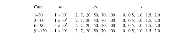
 Ra
 Pr
 s
 Pr=2
 7
 Pr=20
 Pr=50
 100
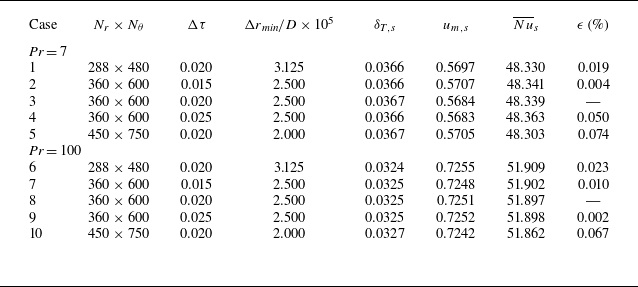
 Ra=108
 s=0
 Δτ
 ϵ
 Nu¯s
 Pr=7
 Pr=100

 ϕ
 uθ
 s=0
 s=2
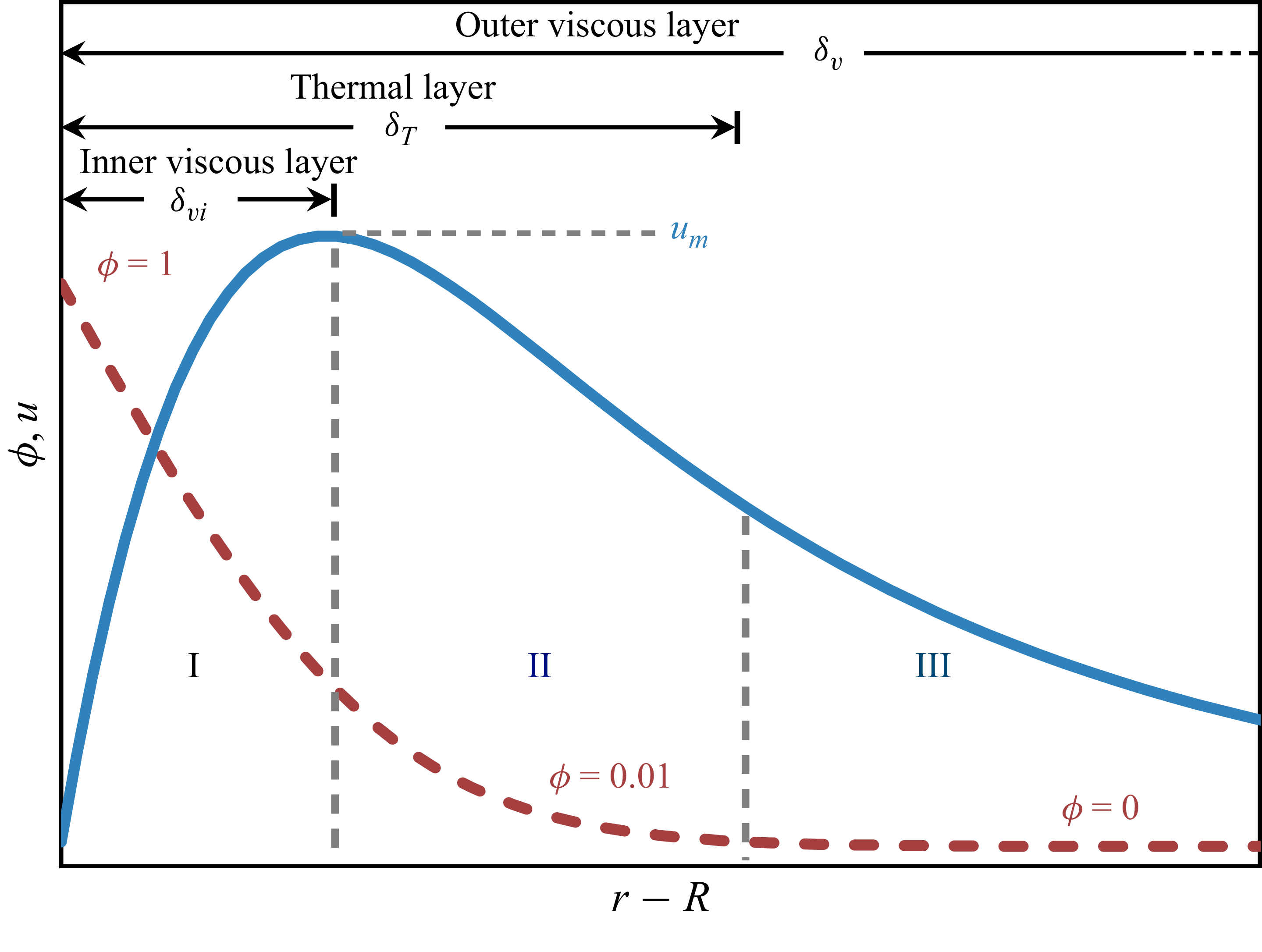
 Pr≳O(1)
 uθ
 ϕ
 r−R

 δT
 Fo1/2
 Ra
 Pr
 s
 θ∈[π/3,2π/3]
 δT=3.68Fo1/2

 T−T∞
 r−D/2
 Ra
 Pr
 s
 ϕ
 η=(r−D/2)/(αt)1/2
 ϕ=erfc(η/2)

 δvi
 Fo1/2(1+Pr−1/2)−1
 Ra
 Pr
 s
 δvi=0.63Fo1/2(1+Pr−1/2)−1

 um
 C(Pr,Pe)
 Ra
 Pr
 s
 Cu=0.087

 uθ
 (r−D/2)/D
 Ra
 Pr
 s
 uθ/um
 ηv=(r−D/2)(1+Pr−1/2)(αt)−1/2
 ηv≃0.63

 δT
 θ
 um
 θ
 s
 um/uref
 θ
 uref=um(θ=π/2)
 Ra
 Pr
 B(θ;s)/B(π/2;s)

 Nu¯
 Fo−1/2
 Ra
 Pr
 s
 Nu¯=0.57Fo−1/2
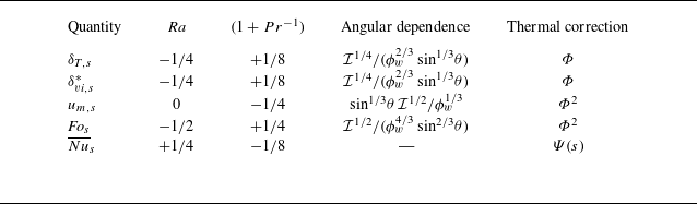
 I(θ)=∫0θϕw5/3(φ)sin1/3φdφ
 δvi,s
 (1+Pr−1/2)−1

 δT
 Fo
 δT/δT,s
 (Fo/Fos)1/2
 δT/δT,s=1
 Fo=Fos

 δT,s
 ξδT,s
 Ra
 Pr
 s
 θ∈[π/18,17π/18]
 δT,s=3.41ξδT,s
 R2=0.998

 δvi,s
 ξδvi,s
 Ra
 Pr
 s
 θ∈[π/18,17π/18]
 δvi,s=2.05ξδvi,s
 R2=0.998

 uθ,s
 (r−D/2)/D
 Ra
 Pr
 s
 uθ,s/um,s
 ηvi,s=(r−D/2)/ξδvi,s
 ηvi,s≃2.05

 um,s
 ξum,s
 um,s=0.62ξum,s
 um,s/um,s(θ∗)
 θ
 s
 f(θ,s)

 Fos
 ξFos
 Ra
 Pr
 s
 Fos=0.22ξFos
 R2=0.995

 Nu¯s
 ξNu¯s=Ra1/4(1+Pr−1)−1/8Ψ(s)
 Ra
 Pr
 s
 Nu¯s=0.53ξNu¯s
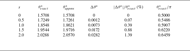
 θ∗
 B(θ;s)
 0≤s≤2
 θexact∗
 θapprox∗
 Δθ∗=θapprox∗−θexact∗
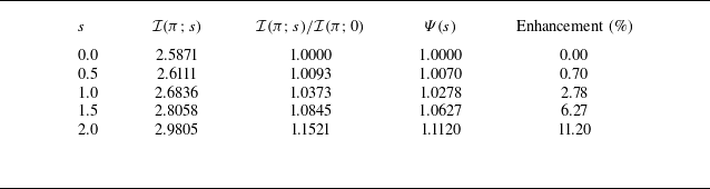
 Ψ(s)
 ϕw(φ)=1+s(φ/π−1/2)
 I(π;s)
 100(Ψ−1)


