1. Introduction

In theoretical population biology, the magnitude and direction of change in population structure are predicted and explained by the distribution of trait fitnesses. But what are trait fitnesses? This question has been the subject of a considerable amount of debate in recent years. The majority opinion is that trait fitness is a causal property. Fitness is (or measures) the propensity of a trait type to change in relative frequency in a population. Accordingly, fitness distribution is a causal propensity of a population: its tendency to undergo selective change. Natural selection, it seems to follow, is a population-level causal process; it is that process caused, and measured, by fitness distribution. Natural selection explanations, then, are causal explanations in that they cite causes of population change. The alternative interpretation is that fitness is a mere statistical, noncausal property of trait types, so fitness distribution is a statistical, noncausal property of a population (Matthen and Ariew Reference Matthen and Ariew2002; Walsh, Lewens, and Ariew Reference Walsh, Lewens and Ariew2002; Walsh Reference Walsh2007). Fitness distribution explains but does not cause the changes in a population undergoing natural selection. This statistical interpretation has been the subject of a considerable amount of comment, mostly negative. My objective is to offer it some support.

I survey three current, competing interpretations of natural selection explanations—the Two-Factor Model, the Single-Factor Model, and the Statistical Interpretation—each of which offers a distinctive account of fitness. The principal commitment shared by the first two interpretations and shed by the Statistical Interpretation is that fitness is a causal property. In fact, these interpretations represent a nested hierarchy of decreasing causal commitment; each one in the list takes on the causal commitments of its successor, plus some extra. My argument involves simply stripping away layers of excess causal commitment. This process of metaphysical divestment terminates at the Statistical Interpretation. Fitness is a noncausal, statistical property of a trait type.

2. Fitness, Variance, and Population Size

Philosophical discussions of fitness often seek to ground trait fitness in the causal capacities of individual organisms (Mills and Beatty Reference Mills and Beatty1979; Sober Reference Sober1984; Bouchard and Rosenberg Reference Bouchard and Rosenberg2004; Rosenberg Reference Rosenberg2006). For example, the fitness of a trait is thought of as the mean (or mean and variance) of the fitnesses of individuals possessing that trait. This approach fosters a very intuitively appealing picture of the explanatory role of fitness. A trait's tendency to change in a population (its fitness) is inherited from the capacities of those individuals that possess the trait. Trait fitness, then, is a sort of summation, or generalization, of the causal contributions of a trait type to the survival and reproduction of the individuals that possess it (Brandon and Beatty Reference Brandon and Beatty1984; Beatty and Finsen Reference Beatty, Finsen and Ruse1989; Beatty Reference Beatty, Keller and Lloyd1992; Haug Reference Haug2007). It is a short step from here to the thesis that trait fitness is itself a causal property of a trait type.

Early models of population dynamics represented the fitness of a trait as the average reproductive output of individuals with the trait. This measure of fitness ignores dispersion around the mean, and it employs the idealizing assumption of infinite population size. Biologists have long known, however, that treating trait fitness in this way has distorting effects: “simply examining the means of all fitness components and applying the classical ideas of selection in finite populations will not be sufficient to make decisions regarding the relative fitnesses of genotypes” (Gillespie Reference Gillespie1975, 410). The reason is that stochastic variation in reproductive output and population size have systematic effects on population dynamics. A number of studies demonstrate that temporal variation in reproductive output has significant implications for change in trait structure of a population (Karlin and Liberman Reference Karlin and Liberman1974; Levikson and Karlin Reference Levikson and Karlin1975; Gillespie Reference Gillespie1977; Orr Reference Orr2007). Where reproductive output varies over time, the fitness of a trait is a function of its mean and variance: “it is well known that when the fitnesses of alleles fluctuate through time natural selection will typically ‘choose’ the allele that shows the best trade-off between average fitness and variance in fitness” (Orr Reference Orr2007, 2997). In such cases, the geometric mean of reproductive output, rather than arithmetic mean, is a more accurate estimate of trait fitness. For a given arithmetic mean, geometric mean decreases as a function of increasing variance (Stearns Reference Stearns2000). The biological (Slatkin Reference Slatkin1974; Stearns Reference Stearns2000) and the philosophical (Beatty and Finsen Reference Beatty, Finsen and Ruse1989; Sober Reference Sober, Singh, Krimbas, Paul and Beatty2001) implications of temporal variation in reproductive output have been discussed widely.

There is another way in which stochastic variation in reproductive output contributes to fitness whose implications, I believe, have not been adequately explored. Gillespie (Reference Gillespie1974, Reference Gillespie1975) demonstrates that where reproductive output varies within generations, variance makes a distinctive contribution to fitness: “the two main properties of the action of selection on the within-generation component of variance in offspring number [are]: (1) Lowering the variance in offspring number will increase the fitness of a genotype. (2) The strength of selection for the variance component is inversely proportional to the population size” (Gillespie Reference Gillespie1974, 602). In the limiting case, where population size is constant, Gillespie tells us that the best measure of fitness of a trait, i, is

(where $\mu _{i}$ is mean reproductive output of i, $\sigma ^{2}_{i}$ is the variance in reproductive output of i within a generation, and n is the population size), “a quantity which depends upon the population size” (604).Footnote ¹

This particular measure of fitness will become important below (sec. 5), but for now the message to carry forward is that both variance in reproductive output and population size are contributory factors in the tendency of a trait to change its relative frequency in a population. These two effects interact; the effect of variance on fitness decreases as an inverse function of population size.

The incorporation of variance and population size into the measure of a trait's fitness does not entail that the fitness value assigned to a trait type is not a summation of the casual contributions of the trait's tokens (Bouchard and Rosenberg Reference Bouchard and Rosenberg2004). But it does entail that trait fitness is not a causal property. By extension, trait fitness distribution is not a cause of population change. Consequently, explanations of population change that cite trait fitness distribution do not cite the causes of population change. At least that is what I intend to argue.

3. Two-Factor Model

Any interpretation of evolutionary explanations must give a satisfactory account of the relation between selection and drift. Selection and drift are discrete, discernible, complementary effects. Selection is the expected population change given the fitness distribution; drift is deviation from expectation. They are independent; selection can occur without drift, drift can occur without selection, or the two can occur in combination. The Two-Factor Model is an attempt to represent this relation utilizing the distinction between process and product. According to the Two-Factor Model, selection and drift are distinguishable as effects (products) because they are, respectively, the consequences of two discrete, composable, proprietary processes (also known as ‘selection’ and ‘drift’; Sober Reference Sober1984; Reference Sober2008, 195ff.; Millstein Reference Millstein2002; Stephens Reference Stephens2004; Shapiro and Sober Reference Shapiro, Sober, Wolters and Machamer2007).Footnote ² They are discrete in the sense that the conditions required for selection to act in a population are wholly different from those conditions required for drift (Brandon Reference Brandon2005). One set of conditions can hold without the other. They are composable in the sense that population change is the consequence of the distinct contributions of selection and drift combined. Finally, selection and drift are proprietary in the sense that what it is for a population change to be selection-the-effect is simply for it to be caused by selection-the-process and similarly, mutatis mutandis, for drift.

Sober (Reference Sober1984) introduces an analogy between selection and drift on the one hand and forces in classical mechanics on the other that illustrates the salient features of the Two-Factor Model. Newtonian forces are the paradigm of discrete, composable causes. The net force acting on a body is the sum of the distinct forces acting severally, each of which could act independently of the others. Newtonian mechanics offers a way of decomposing this net cause into component causes. While this Newtonian analogy has drawn extensive criticism—selection and drift are not literally forces—it retains a certain heuristic value. Stephens (Reference Stephens2004) defends the Newtonian analogy in the following way: “Evolutionary theory is analogous to Newtonian mechanics in many ways. In particular it makes perfect sense to think of selection, mutation, migration and drift as causes since they are factors that make a difference. … Furthermore these causal factors can often combine in Newtonian ways, with one factor canceling out or augmenting the effect of another” (568; emphasis in original).

Support for the analogy comes from the observation that the putative processes of selection and drift are distinct difference makers. Each bears a different invariance relation to population change. The amount of selection in a population varies as a function of the degree of variation in fitness. The amount of drift varies as a function of population size (Stephens Reference Stephens2004). So, it looks as though we have two independently measurable, composable causes of population change: selection and drift. “We view selection and drift as distinct processes whose magnitudes are represented by distinct population parameters (fitnesses on the one hand, effective population size on the other)” (Shapiro and Sober Reference Shapiro, Sober, Wolters and Machamer2007, 261). This is the crux of the Two-Factor Model. It is a simple, compelling idea, and it has considerable currency among philosophers of biology (Stephens Reference Stephens2004; Reisman and Forber Reference Reisman and Forber2005; Millstein Reference Millstein2006; Abrams Reference Abrams2007b; Shapiro and Sober Reference Shapiro, Sober, Wolters and Machamer2007; Lewens Reference Lewens2009).

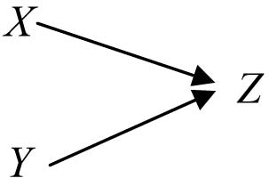
Recent work on interventionist approaches to causation, at first blush, appears to bear out the Two-Factor Model. On the interventionist approach, manipulability is the mark of a cause (Woodward Reference Woodward2003). A factor, X, is a genuine cause of some effect, Z, only if an intervention that changes the value of X (i.e., manipulating it) would bring about a systematic change in the value of Z. A two-factor causal model might be depicted as in figure 1. In the figure, X and Y are causes of Z just if there is a change-relating invariance relation between X and Z and a different invariance relation between Y and Z, and interventions on X and Y each bring about a change in the value of Z (Woodward Reference Woodward2003). Where X and Y are probabilistic causes, the following equation expresses the causal relations of the system:

In (2), aX and bY represent the functional relation between X and Z and Y and Z, respectively; they give us the expected values of Z given the values of X and Y;Footnote ³ U is the error term.

Figure 1.

Diagram of a two-factor causal model.

Reisman and Forber (Reference Reisman and Forber2005) argue that this sort of model fits the relation between selection (X), drift (Y), and population change (Z) perfectly. Manipulating fitness distribution alters the expected outcome of population change. Manipulating population size changes the likelihood of the outcome of selection diverging from expectation.

The authors illustrate this claim with a series of experiments performed by Dobzhansky and Pavlovsky (Reference Dobzhansky and Pavlovsky1957) in which population size is manipulated. Reisman and Forber show that these interventions have distinct, discernible effects on population change, precisely the effects predicted by the two-factor causal model. Manipulating fitness distributions is also a commonplace evolutionary experiment. It too leads to precisely the sort of differences in population change that the Two-Factor Model predicts. Shapiro and Sober strongly endorse the argument from manipulability: “If you intervene on fitness values while holding fixed population size, this will be associated with a change in the probability of different trait frequencies in the next generation. And the same is true if you intervene on population size and hold fixed the fitnesses” (Reference Shapiro, Sober, Wolters and Machamer2007, 261). Lewens concurs: “Since both the selection and drift can be manipulated in ways that have systematic impacts on population outcomes, both selection and drift are causes” (2009, 8).

The Two-Factor Model, then, looks to be on firm footing, but it has two significant flaws. The first is that it misapplies the interventionist criterion for causes. The second is that it fails in its principal objective, to capture the required distinction between selection and drift as effects. The account of trait fitness given above brings both of these deficiencies into focus.

Demonstrating an invariance relation between X and Z on the one hand and Y and Z on the other is not sufficient to confirm the Two-Factor Model depicted in figure 1. In addition, these relations also need to be modular (Woodward Reference Woodward2002, Reference Woodward2003). “If we make the … plausible assumption that a necessary condition for two mechanisms to be distinct is that it be possible (in principle) to interfere with the operation of one without interfering with the operation of the other and vice versa, we have a justification for requiring that systems of equations that fully and correctly represent a causal structure should be modular” (Woodward Reference Woodward2003, 48). Formally, modularity is a property of a system of equations (Woodward Reference Woodward2003). The equation that describes the Two-Factor Model in figure 1, equation (2),

is modular if and only if we can intervene only on the value of Y without altering the value of X; conversely, we can intervene only on the value of X without altering the value of Y. The terms X and Y are discrete causes of the value of Z only if (2) is modular.

The conception of fitness given above demonstrates that where X is fitness distribution (the putative cause of selection) and Y is population size (the putative cause of drift), equation (2) is not modular. The reason is fairly obvious. Fitness is a function of mean reproductive output, variance, and population size. Manipulating population size (Y) affects fitness distribution (X). Given two traits with the same mean reproductive output ($\mu _{i}$) but different variance, their fitnesses will diverge if we decrease population size and converge if we increase population size. Thus, a manipulation of population size (Y) is eo ipso a manipulation of fitness distribution (X). This is no mere aberrant case; wherever there is variation among the trait fitnesses, intervening on population size will change the fitness distribution.Footnote ⁴ Consequently, equation (2) is not modular. The relation between fitness distribution (the putative mechanism of selection) and population size (the putative mechanism of drift) cannot be as depicted in figure 1. Selection and drift are not discrete causes of population change as the Two-Factor Model contends.

Clearly the experiments cited by Reisman and Forber (Reference Reisman and Forber2005) demonstrate that manipulating population size has consequences for the kind and degree of population change. But the experiments do not show that fitness distribution and population size can be manipulated independently. Thus the experiments cited by Reisman and Forber do not support the Two-Factor Model.

The failure of modularity has two sorts of adverse implications for the Two-Factor Model. First, it demonstrates that the Two-Factor Model fails on its own terms. It fails to represent selection and drift as discrete, independent causes of population change. They are not discrete because the putative mechanism of drift (population size) is a determinant of the mechanism of selection (fitness distribution). They are not independent in the sense that wherever there is variation in trait fitnesses, one cannot intervene on drift without also affecting the process of selection.

Second, the Two-Factor Model also fails to fulfill the principal desideratum of any interpretation of evolutionary explanations. It fails to distinguish between selection and drift as effects. As characterized by the Two-Factor Model, selection and drift the effects are distinguished by being (respectively) the products of proprietary processes of selection and drift. But, given the contribution of population size to fitness distribution, one can bring about a change in selection-the-effect by manipulating population size, the putative mechanism of drift-the-process. It is an unfortunate consequence of the Two-Factor Model that drift-the-process causes selection-the-effect.

There is a simpler, more obvious objection to the Two-Factor Model that does not rely on the interventionist conception of causation or any particular account of fitness. On any causal interpretation, the relation between fitness distribution, however it is characterized, and population change is a probabilistic one. In the above model it is written as

(eq. [2]), where $aX$ is the functional relation between fitness distribution and population change, Z, and U is the error term. The concept of drift was introduced into evolutionary theory precisely to play the role of the error term (Wright Reference Wright1931). If drift is to have a role in this model, then priority and common usage demand that it be assigned the role of the error term, U, and not $bY$. The extra term in the Two-Factor Model, $bY$, is completely otiose.

The same considerations apply equally to any variant of the Two-Factor Model. Millstein (Reference Millstein2002, Reference Millstein2006), for example, proposes that there are two distinct kinds of population-level causal processes, discriminate sampling and indiscriminate sampling.Footnote ⁵ Discriminate sampling—selection—occurs when individuals with variant trait types in a population vary in their propensity to be ‘sampled’ (i.e., to survive or reproduce). Indiscriminate sampling—drift—occurs when individuals of different trait types do not differ in their propensity to be sampled. Discriminate sampling is a probabilistic cause, on this view, so selection is a probabilistic cause. The equation that describes the relation between selection and population change needs an error term. The traditional role assigned to drift is that of the error term. So even if there is a separate process of indiscriminate sampling, it is not drift (Brandon Reference Brandon2005).

The distinguishing feature of the Two-Factor Model is that it represents drift as a distinct cause of population change, independent from selection. But this is a misconstrual. Drift was only ever intended as error. In a probabilistic causal model, error is not an additional cause. Not only is positing a separate causal term for drift superfluous, it is misleading.

4. Single-Factor Model

This suggests an alternative causal interpretation. The Single-Factor Model takes fitness distribution to be a probabilistic propensity of a population (Ramsey and Brandon Reference Ramsey, Brandon, Ruse and Hull2007), but drift is not a separate cause; it is just error.Footnote ⁶ “Drift is any deviation from the expected levels due to sampling error. Selection is differential survival and reproduction that is due to … expected differences in reproductive success” (Brandon Reference Brandon2005, 168–69). Certainly the Single-Factor Model observes the intended usage of the concept of drift while preserving the presumed causal role of selection. The Single-Factor Model has other virtues, too; another analogy serves to highlight them.

4.1. The Regression Analogy

Where the Two-Factor Model explicitly draws an analogy with Newtonian mechanics, the Single-Factor Model suggests another, more germane analogy for the relation between trait fitness distribution, drift, and population change. The relation between population change and fitness distribution is relevantly like the relation between the ‘response’ and ‘explanatory’ variables in a linear regression.Footnote ⁷ A linear regression equation of the form

describes a line through the scatter of points that plot the values of two variables, y and x, against each other. In (3), y is the response variable, x is the explanatory variable, a describes the slope of the regression line, and b is the y intercept. (Hereafter, I shall assume that b passes through the origin and drop the b term.) The regression line minimizes the sum of the errors (squared) along the y axis. It is the line that best represents the dependence of y on x.

For any given point i in the scatter plot, the y-value can be thought of as composed of two values:

where $ax_{i}$ is the expected value generated by the functional relation between y and x, and $\varepsilon _{i}$ is the divergence of $y_{i}$ from the expected value—that is to say, error. The relations between change in a given population, fitness distribution, and drift are analogous to those between $y_{i}$, $ax_{i}$, and $\varepsilon _{i}$, respectively. The $ax_{i}$ term represents the effect of fitness distribution on population change: ‘selection’ in a word. This relation generates an expected outcome for population change. The difference between this expected outcome and the observed, $y_{i}$, is $\varepsilon _{i}$—drift.

The analogy captures certain important features of the relation between selection and drift in a way that the Two-Factor Model signally failed to do. Under certain plausible assumptions, the functional relation in a regression, $ax_{i}$, makes no prediction about the direction or magnitude of $\varepsilon _{i}$ (and of course the converse relation holds). The expected outcome, $ax_{i}$, and error, $\varepsilon _{i}$, are thus independent in the same way that selection and drift are said to be. The regression analogy also captures a further important feature of drift. As noted, there is a predictable relation between the magnitude of drift and population size. Drift is larger in small populations.Footnote ⁸ This is to be expected if drift is the sort of statistical error we find in regression analyses. Statistical error increases with decreasing sample size. But there is no temptation to think of this relation as causing a particular error value. When an individual value, $y_{i}$, deviates from the expected outcome, $ax_{i}$, one does not think of the error, $\varepsilon _{i}$, as being caused by the sample size.

It is tempting to think of the equation that describes the value of $y_{i}$ in a regression relation,

as an instance of the single-factor probabilistic causal relation

This is the essence of the Single-Factor Model. Fitness distribution is a probabilistic cause of population change. Drift is the error term.

5. Simpson's Paradox

Simpson's paradox is one of the potential pitfalls of inferring causes from probabilistic relations.Footnote ¹⁰ It occurs when for some putative cause C and its effect E,

Yet, for some exhaustive division of the population into subpopulations, $F_{1},\,\ldots, \,F_{n}$, for each subpopulation, $F_{i}$,

The reversal of probabilistic inequalities in (5) and (6) is known as a ‘Simpson's reversal’. Simpson's reversal is a benign, workaday probabilistic phenomenon. It causes difficulties only when we attempt to draw causal inferences from the probabilistic inequalities.

It is easy to illustrate the discomfiture that Simpson's reversal, like the one found in (5) and (6), can introduce into causal reasoning. Consider the Paradox of the Perplexing Painkiller. A series of drug trials suggest that, in the population overall, the probability of recovering from a headache, E, is raised by treatment with some new analgesic drug, C, as in (5). The results also show that when the test sample is divided up according to sex, the probability of nontreated patients recovering is higher than the probability of treated patients recovering for both men and women, as per (6). A physician attempting to use these results in her clinical practice would encounter some peculiar problems. If a patient comes into her clinic complaining of the ailment and the physician does not know the sex of the patient, then she should treat her patient as a representative of the population as a whole, in which case the results suggest that she should administer the drug (by [5]). At the same time, she knows that the patient is either male or female; if the patient is male, she should not administer the drug (by [6]), and if the patient is female, she should not administer the drug either (by [6]). So, on the one hand, what the physician does not know about her patient changes her view on the effectiveness of the drug. At the same time she knows (from [6]) that what she does not know is irrelevant to the effectiveness of the drug. Something has gone wrong. Our physician has an incoherent set of causal beliefs. She is embroiled in a Simpson's paradox.

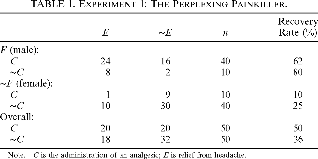
Pearl (Reference Pearl2000) offers an example illustrating how this sort of Simpson's reversal can arise and how the paradox can be resolved. Table 1 gives some hypothetical results from the problematic drug trials adapted from his discussion. There is clearly a reversal of probabilistic inequalities here, as can be seen by comparing the recovery rates in the subpopulations (F, ∼F) and overall.

Table 1.Experiment 1: The Perplexing Painkiller

	E	∼E	n	Recovery Rate (%)
F (male):
C	24	16	40	62
∼C	8	2	10	80
∼F (female):
C	1	9	10	10
∼C	10	30	40	25
Overall:
C	20	20	50	50
∼C	18	32	50	36

Note.—C is the administration of an analgesic; E is relief from headache.

One of the causes of the reversal is the inequality among the sample sizes between treatments. In experiment 1, treated males (40) made up 40% of the sample, and untreated males made up 10%; untreated females constitute a further 40%, and treated females account for only 10%. Overall recovery rates are skewed by the fact that 80% of those who took the drug probably would have recovered whether they had or not and 80% of those who did not take the drug probably would not have recovered either way. Had sample sizes been equal between cells, then assuming the recovery rates shown in the table, the overall recovery rates would have been $C=27\% $, $\sim C=53\% $—no reversal. Sample bias seems to be a prevalent problem in meta-analyses of drug trial statistics. A study can inoculate itself against an unwanted Simpson's reversal by ensuring that sample sizes are constant between treatments (Hanley et al. Reference Hanley, Thériault, Reintjes and Boer2000).

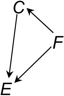
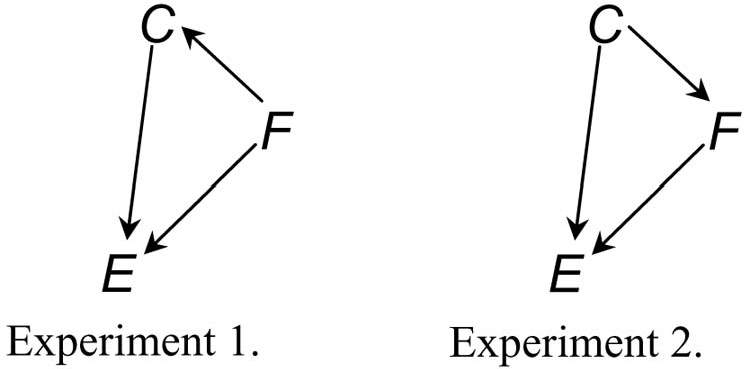
Still, this prophylactic measure is not always available. In cases in which the reversal of probabilistic inequalities does occur, we need a procedure for deciding which probabilities can be interpreted as causal and which cannot. Pearl (Reference Pearl2000) tells us that we can use auxiliary information about the causal structure of the experiment as a guide. For example, we know a few things about sex and drugs, such as that taking an analgesic typically does not cause one's sex. So being a member of F or ∼F is causally independent of the treatment, C. But being male or female can have consequences for the probability of undergoing treatment. In this experiment, males are more likely than females to undergo treatment: $P(C\vert F) =.64> P(C\vert \sim F) =.20$. Sex can also have consequences for the likelihood of recovery. Table 1 shows that males are more likely to recover than females whether or not they take the drug: $P(E\vert F) =.60 > P(E\vert \sim F) =.22$. Pearl depicts the causal structure of this experiment as in figure 2. The property that distinguishes the subpopulations has independent consequences for both the probability of C and the $P(E\vert C) $. The term F is a confounding factor. The ‘overall’ result fails to take this into account. Pearl suggests that we should consider the overall result, $P(E\vert C) =.50> P(E\vert \sim C) =.36$, a statistical artifact. We should infer that this drug does not relieve the affliction in the population overall.

Figure 2.

The causal relations between treatment with an analgesic, C, sex, F, and recovery from headache, E, in experiment 1.

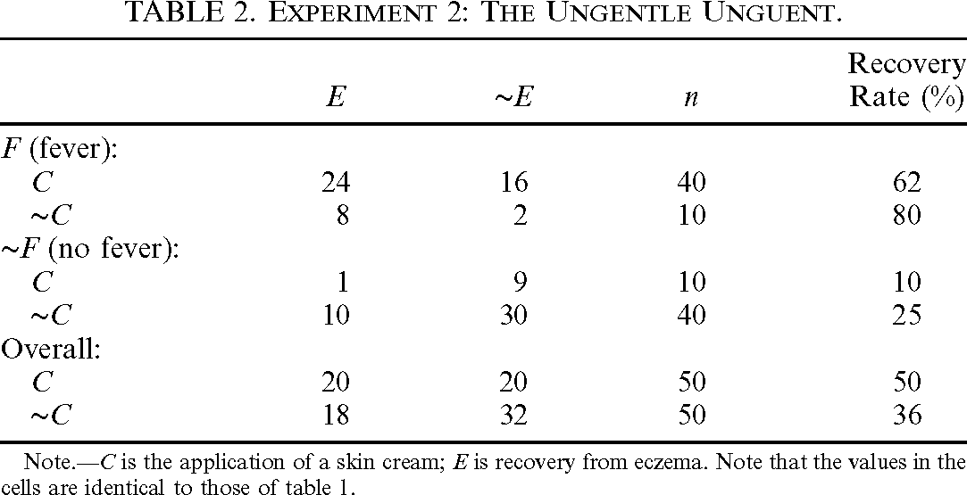
The moral to be drawn from this story is not that whenever there is a Simpson's reversal the overall effect is an artifact. Nor is it that wherever there is a Simpson's reversal some of the probabilistic relations must be noncausal. A minor change to the above example demonstrates this. Consider the unparadoxical case of the Ungentle Unguent. We are testing the efficacy of a skin cream (C) as a cure for eczema (E). We find that some of the treated subjects develop a fever (F), more than we would expect. The results are given in table 2.

Table 2.Experiment 2: The Ungentle Unguent

	E	∼E	n	Recovery Rate (%)
F (fever):
C	24	16	40	62
∼C	8	2	10	80
∼F (no fever):
C	1	9	10	10
∼C	10	30	40	25
Overall:
C	20	20	50	50
∼C	18	32	50	36

Note.—C is the application of a skin cream; E is recovery from eczema. Note that the values in the cells are identical to those of table 1.

The results are exactly as they were in the analgesic experiment. Nevertheless, we should not conclude from this experiment that the overall result is a statistical artifact, as we did in experiment 1. The difference between experiment 1 and experiment 2 resides in the relation between F and C. In each experiment, the relation is expressed as

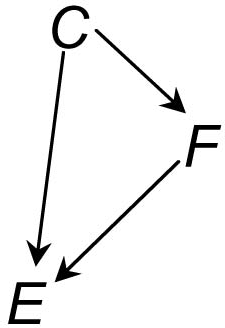
But whereas in experiment 1 the relation is not causal, in experiment 2 it is at least plausible to suppose that it is. Administering the cream, C, causes fever, F. In experiment 2, the treatment, C, changes the distribution of the subpopulations, F. It causes some subjects to be in subpopulation F who would not otherwise be there. The treatment causes fever, and fever independently raises the chances of recovery, E. The causal structure should be depicted as in figure 3. The overall result is not an artifact. It represents the amalgam of two distinct causal paths from C to E. The physician faced with these test results should administer the drug. She knows that it stands a reasonable chance of working, albeit through the ungentle means of inducing a fever.

Figure 3.

The causal relation between skin cream, C, fever, F, and relief from eczema, E, in experiment 2.

This scenario is similar to one discussed by Cartwright (Reference Cartwright1979) in which smoking (C) raises the chances of heart disease (∼E) in those who exercise (F) and those who do not (∼F). Yet smoking is positively correlated with exercise, and exercise prevents heart disease. It is reasonable in these cases to interpret both the within-group effect and the overall effect as expressive of causal relations between C and E. Simpson's reversal occurs in these cases, but there is nothing paradoxical about interpreting all the conditional probabilities as representing causal relations.

The difference between the pathological cases of Simpson's reversal (experiment 1) and the benign ones (experiment 2) is entirely extrastatistical; it resides in their causal structures. One lesson to be learned is that conditional probabilities alone do not give us causal structure (Cartwright Reference Cartwright1994). Another is that the indiscriminate interpretation of conditional probabilities as causal relations can lead to incoherence.

The Sure Thing Principle. It would help us to avoid the incoherences if we knew why the pathological cases are paradoxical and why we so easily succumb to them. Pearl (Reference Pearl2000) attributes our susceptibility to the paradoxes to a generalized human—perhaps, better, a ‘Humean’—psychological proclivity to interpret the probabilities in the ‘calculus of proportions’ by default as probabilities in the ‘calculus of causes’: “humans are generally oblivious to rates and proportions … and … constantly search for causal relations. … Once people interpret proportions as causal relations, they continue to process those relations by causal calculus and not by the calculus of proportions. … Were our minds governed by the calculus of proportions, … Simpson's paradox would never have generated the attention that it did” (181). The principal difference between the ‘calculus of causes’ and the ‘calculus of proportions’ is that the reversal of probabilistic inequalities is consistent with the calculus of proportions and sometimes inconsistent with the calculus of causes. More precisely, the calculus of causes is constrained by the Sure Thing Principle.

When causal inferences violate STP, we have an incoherent set of causal beliefs. This is readily apparent in the Paradox of the Perplexing Painkiller (experiment 1). Here, an action, C (administering the drug), that increases the probability of nonrecovery, ∼E, in each subpopulation decreases it overall. Interpreting the probabilities in the Ungentle Unguent (experiment 2) example as causal relations, however, is consistent with STP. STP is not violated by experiment 2 because the proviso is not met: administering the treatment, C, changes the distribution of the subpopulations, F (by raising the chances of fever). A quick comparison of figures 2 and 3 confirms the difference (in fig. 4).

Figure 4.

Experiment 1: ‘the Perplexing Painkiller’. F is causally independent of C. The action C does not affect the distribution of the subpopulations, F and ∼F. Experiment 2: ‘the Ungentle Unguent’. F is causally dependent on C. The action C changes the distribution of the subpopulations, F and ∼F.

STP gives us a procedure for diagnosing and remedying cases of Simpson's paradox. The diagnostic procedure goes as follows. We ask (i) “is there a reversal of probabilistic inequalities?” (first clause of STP) and (ii) “is the proviso upheld?” (second clause of STP). If the answers to questions i and ii are both “yes,” we have a violation of STP. Interpreting the probabilities as causal relations will yield an incoherent set of causal commitments. Some of the conditional probabilities must be noncausal.

With a little extrastatistical or causal information, Simpson's paradoxes can generally be resolved. Equalizing the treatment sample sizes or attending to the causal structure of the experiment can usually direct us toward a coherent causal interpretation. It is conceivable, however, that for some Simpson's reversals there is no plausible causal interpretation of the probabilities that is consistent with STP. In such a circumstance, there is no coherent causal interpretation to be had. I believe that this kind of scenario can be constructed for the causal interpretation of fitness.

6. Simpson Meets Gillespie

We saw from the Gillespie account of fitness that where there is within-generation variation in reproductive output, fitness is a function of mean and variance of reproductive output and population size. In the case of populations of constant size, fitness is to be estimated as

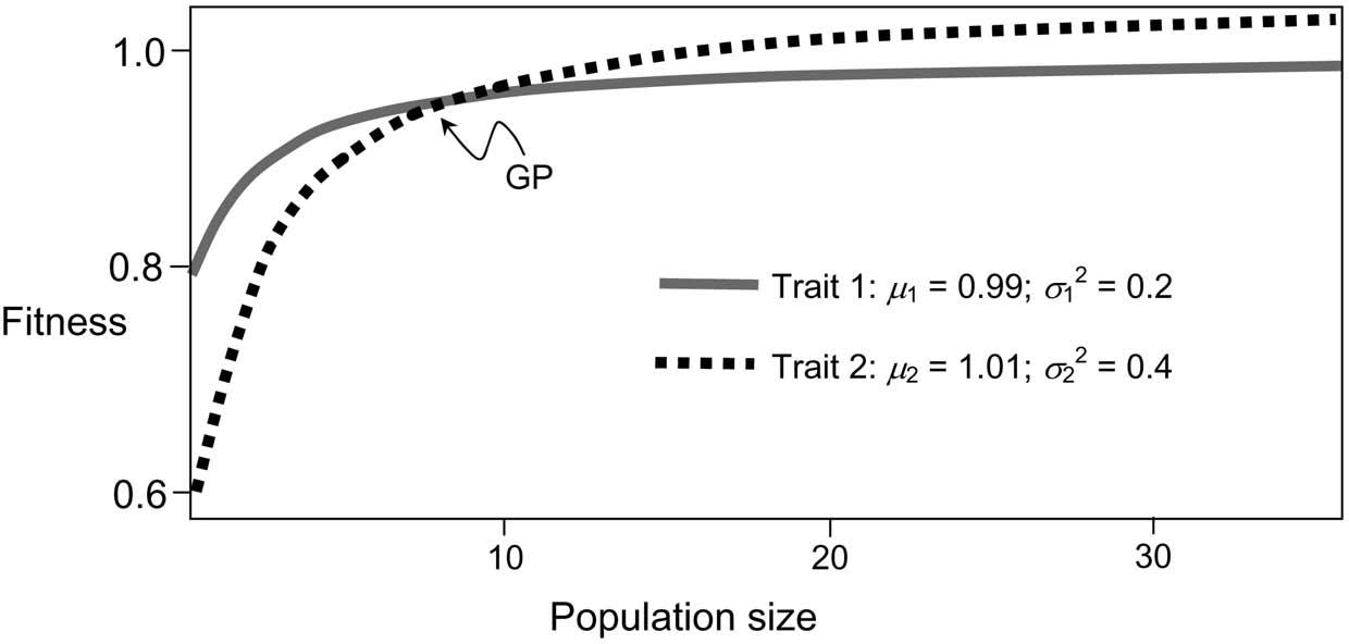
(Gillespie Reference Gillespie1975, Reference Gillespie1977). The following model illustrates the significance of the influence of size and variance on fitness. Let the distribution of reproductive outputs be as follows:Footnote ¹¹

The fitnesses of traits 1 and 2 can be plotted against population size as in figure 5. I call GP the ‘Gillespie Point’; it is the population size ($n=10$) at which $w_{1}=w_{2}$. Below the Gillespie Point, trait 1 is fitter than trait 2; above it, trait 2 is fitter than trait 1.

Figure 5.

Fitness as a function of population size (for within-generation variation in reproductive output).

Suppose that we have a homogeneous population, characterized as in figure 4, comprising 14 subpopulations of six individuals each, in such a way that each has individuals of both trait 1 and trait 2. In each of these subpopulations, i, the fitness of trait 1 exceeds that of trait 2:

As long as the distributions of reproductive outputs (the $\mu _{i}$'s and $\sigma ^{2}_{i}$'s) in the population overall are representative of the subpopulations, in each subpopulation, it will be more likely that trait 1 increases in frequency relative to trait 2 than vice versa. We are impelled to say that in each subpopulation there is selection for trait 1 over trait 2. In the population overall, however, the fitness of trait 2 exceeds that of trait 1:

There is selection for trait 2 over trait 1.

Clearly, (8) and (9) constitute a Simpson's reversal. To illustrate this, we adopt our previous notation: let E be trait 2 increases and C be the within-population fitness distribution ($w_{1}> w_{2}$). Let ∼C be the null hypothesis—H₀: $w_{1}\leq w_{2}$—and let the $F_{i}$'s be the subpopulations:Footnote ¹²

Here I have stipulated, by analogy with the medical experiments, that the overall population is the aggregate of the subpopulations, but it is worth noting that any way of composing the populations out of subpopulations of $n\leq 10$ (in which it makes sense to assign fitnesses to both traits) will produce the same reversal.

It is important to note that it is irrelevant to the example quite how the subdivision of the populations is achieved. The subpopulations might be isolated from one another by barriers. By the same token, they might just be replicates of the same experimental setup or simply just a redescription of the population. It is legitimate for biologists to investigate the dynamics of whole populations and their subpopulations, howsoever the latter are demarcated.

The causal interpretation of fitness enjoins us to read the probabilistic relation between fitness distribution and population change as causal. When the fitness of trait 1 exceeds the fitness of trait 2, expressions (10) and (11), there is an ensemble-level causal process—selection—that causes trait 1 to grow faster than trait 2. The causal interpretation of fitness, then, is committed to saying that within each subpopulation selection (probabilistically) causes trait 1 to increase relative to trait 2. But the aggregate of these subpopulation causes causes trait 2 to increase relative to trait 1. This looks like a Simpson's paradox. Even if perchance it isn’t, it is definitely a prima facie violation of STP. An action C (selection of trait 1 over trait 2) that raises the probability of some effect E (the preponderance of trait 1 over trait 2) in each subpopulation lowers the probability of E overall.

The causal interpretation has some work to do. There are two options. The first is to explain away either the subpopulation probabilities or the overall probability as an artifact, as was done in the Paradox of the Perplexing Painkiller. The second is to demonstrate that there is no violation of STP after all, as we did in the case of the Ungentle Unguent.

The first strategy looks hopeless; the usual remedies provide no relief here. For example, the reversal cannot be attributed to skewed sample sizes. The subpopulations are all the same size. Thus there is no ‘illegitimate averaging’ across unequal treatments.Footnote ¹³ Nor can it be argued that there is a differential effect of subpopulation membership, F, on the value of C as there was in the Perplexing Painkiller case (see table 1 and fig. 1). In that instance, the reversal is attributable to the fact that the property that distinguishes F (being male) raises the probability of C, E, and $E\vert C$, whereas the property that distinguishes ∼F (being female) lowers $P(C) $, $P(E) $, and $P(C\vert E) $. But our biological population is relevantly different in three respects. First, there is no difference in the value of the putative causal parameter, C, between subpopulations. So the reversal of probabilistic inequalities cannot be attributed to some independent causal factor that differentially affects C in each treatment. Second, the only plausible property of subpopulations, F, that could influence fitness distribution, C, is subpopulation size. Subpopulation size does have an influence on C, but this relation is constitutive, not causal. As we saw in section 3, intervening on population size does not cause a change in fitness distribution; it just is a change in fitness distribution. Third, it is incoherent to suppose that the effect of subpopulation size on fitness distribution is causal, on pain of incurring another violation of STP. If F (dividing the population into equal subpopulations) raises the chances of C in every subpopulation equally and C raises the chances of E in each subpopulation, then F raises the chances of E in each subpopulation. So F raises the chances of trait 1 increasing over trait 2 in each subpopulation, expressions (10) and (11), but lowers chances of trait 1 increasing over trait 2 overall, expression (12). This is yet another violation of STP.

This is disanalogous to the Paradoxical Painkiller experiment, in which F (being male) raises the recovery rate in all subpopulations (both treated, C, and nontreated, ∼C) and raises the recovery rate overall: no Simpson's reversal here. This is why it is coherent to interpret being male as a cause of recovery in experiment 1 but incoherent to interpret subpopulation membership as a cause of population change. The upshot is that one cannot salvage the causal interpretation by explaining away the reversal of fitness inequalities as a statistical artifact.

More important, however, we should not want to explain away the reversal of fitness inequalities. There is nothing spurious about either the subpopulation fitness distribution or the overall population distribution. For any subpopulation of $n< 10$, trait 1 really is more likely to increase relative to trait 2. In the population overall, trait 2 really is more likely to increase relative to trait 1. It may not be entirely clear how this is possible. It occurs because at small population sizes trait 2 loses out to trait 1 more frequently than it wins. But because the mean of trait 2 is higher, when it increases with respect to trait 1, it tends to do so by a greater margin than when it decreases relative to trait 1. Aggregating trait 2's frequent, small ‘losses’ and infrequent, large ‘wins’, we get more trait 2's than trait 1's overall but more subpopulations in which trait 1 increases relative to trait 2.Footnote ¹⁴ This outcome is correctly predicted by the subpopulation fitnesses and the overall fitnesses. There is nothing pathological about the reversal of probabilistic inequalities.

The challenge for the causal view of fitness, then, is to articulate a coherent interpretation in which, within each subpopulation, fitness distribution causes trait 1 to increase over trait 2; yet in the population overall, fitness distribution causes trait 2 to increase over trait 1.

One strategy for relieving the Simpson's paradox is to invoke the proviso stated in STP: namely, “provided that the action does not change the distribution of the subpopulations” (Pearl Reference Pearl2000, 181; emphasis added).Footnote ¹⁵ If the proviso is not met, the Sure Thing Principle is not violated. In that case, interpreting the reversal of probabilistic inequalities as a reversal of causal relations is consistent with STP. But this defense of the causal interpretation of fitness is futile. The proviso is clearly upheld. Fitness distribution within the subpopulations, C, does not change subpopulation size, F. The relation between fitness and population size is not analogous to the relation between applying the cream, C, and fever, F, in the Ungentle Unguent example or the relation between smoking, C, and exercise, F, in Cartwright's (Reference Cartwright1979) scenario. In the biological example, C does not cause E by causing some intermediate effect F. The proviso offers no succor to the causal interpretation.

The only strategy remaining to the causal interpretation is to posit two distinct (types of) selection processes: one that operates within subpopulations (call it ‘selection_w’) and another that operates across the population overall (call it ‘selection_o’). The first tends to cause trait 1 to increase in frequency relative to trait 2. The second tends to increase the frequency of trait 2 relative to trait 1.Footnote ¹⁶ Here the defender of the causal interpretation must make a choice: either the process of selection in the population overall is independent of the processes of selection occurring within the subpopulations or it isn’t. If the within-group and overall causes are independent, then there should be no worries about violations of STP. Unfortunately, selection_o is not independent of selection_w. If it were, we could manipulate selection_o while leaving selection_w unchanged. But this is impossible. Any intervention on the overall fitness distribution (selection_o) is an intervention on some within-group fitness distribution.Footnote ¹⁷ That in turn affects selection_w. So selection_o supervenes on selection_w: selection_o is just the aggregate of the selection_w's.Footnote ¹⁸ If selection_o and selection_w are causes, then their relationship is subject to the Sure Thing Principle. But in our model they violate the Sure Thing Principle. So they cannot both be causes.

The upshot is that in our Gillespie model, interpreting the conditional probabilities in the calculus of causes induces an inconsistent set of causal commitments. There is no causal interpretation of the fitness distributions that does justice to their explanatory role and is consistent with the Sure Thing Principle. Consequently, interpreting fitness distributions as causes leads to an incoherent set of causal commitments.

It is perfectly coherent, however, to interpret the probabilistic relation between fitness distribution and population change in the calculus of proportions. Fitness distributions correlate with, but do not cause, the population changes they explain. Interpreting fitnesses as mere statistical correlations has the distinct advantage of allowing us to hold on to all the genuinely explanatory probability relations. It allows us to maintain consistently that within each subpopulation, trait 1 is likely to increase over trait 2, (10) and (11), but in the population overall, trait 2 is likely to increase over trait 1, (12). Any other interpretation of the probabilities fails to do justice to the predictive and explanatory roles of fitness.

Not only should this result relieve us of any lingering inclination to interpret fitness, and the explanations it figures in, along the lines of the Two-Factor Model, it should put paid to the Single-Factor Model too. The feature of that model that distinguishes it from the Statistical Interpretation is that the Single-Factor Model interprets the relation between fitness distribution and population change as causal, whereas the Statistical Interpretation takes it to be a mere statistical correlation. Given the flaws of the Two-Factor and Single-Factor models, the only candidate left standing is the Statistical Interpretation. It is the interpretation that remains after the excess causal commitments of, first, the Two-Factor Model and then the Single-Factor Model are stripped away. These extra commitments are mere metaphysical excrescences and should be removed from our interpretation of evolutionary theory.

7. Conclusion

If the argument above is correct, fitness distribution explains but does not cause population change. In essence, the argument is that three theses constitute an inconsistent triad. These are (i) the conception of fitness in which variance and population size play a role, (ii) the Sure Thing Principle, and (iii) the causal interpretation of trait fitness. My claim is that iii, the causal interpretation of trait fitness, is the culprit. No doubt this conclusion will be uncongenial to some. Anyone seeking to resist the conclusion might choose instead to deny either i, the conception of fitness, or ii, the Sure Thing Principle. But these are drastic measures and are distinctly unpalatable.

The fitness concept I have employed is not so easy to gainsay. There is ample empirical evidence and theoretical support for the thesis that variance in reproductive output and population size have systematic effects on population dynamics in the way I have described (Gillespie Reference Gillespie1974, Reference Gillespie1975, Reference Gillespie1977; Karlin and Liberman Reference Karlin and Liberman1974). Denying the contribution of variance and population size to fitness would constitute an ad hoc revision of well-confirmed scientific practice.

Similarly, the cost of repudiating ii, the Sure Thing Principle, is inordinately high. STP is thought to capture a deep-seated feature of our common intuitions about causation. It is also a direct consequence of the intuitions that motivate the interventionist approach to causation (Pearl Reference Pearl2000). So one could not, on the one hand, appeal to the interventionist accounts of causation, as many causal theorists have done, while denying STP. Furthermore, STP plays a pivotal role in guiding causal inferences. Compliance with STP allows us to distinguish the pathological cases of Simpson's reversal from the benign ones. The repudiation of STP would adversely affect our ability to make reliable causal inferences from statistical data. If one is faced with the inconsistent triad, the most prudent course of action is to deny iii, the causal interpretation of trait fitness. As we have seen, the arguments adduced for it are weak. It is certainly not a sure thing.

If trait fitness is a statistical correlate and not a cause of population change, then explanations that cite it are noncausal, statistical explanations. I suspect that the causal interpretation derives much of its appeal from the intuition that to explain an occurrence one must cite its causes (Salmon Reference Salmon1984). If only causes explain and fitness distribution is not a cause, then one might be tempted to conclude that fitness distribution does not explain.Footnote ¹⁹ Little, however, aside from philosophical prejudice, supports this view. Biologists appear to use fitness distribution as an explanatory concept, and it appears adequate to the task. Fitness offers us an account of why one trait changes in frequency relative to another, why one population's trajectory differs from another, even why population size has a systematic effect on population dynamics. Denying that trait fitness distribution genuinely explains requires a drastic, ad hoc revision of scientists’ explanatory practices.

If the statistical interpretation of evolutionary explanations is correct and biologists’ use of fitness is genuinely explanatory, then the dictum that only causes explain must be wrong. Demonstrating the intuition to be mistaken is one thing—a counterexample suffices. Showing why it is wrong is quite another. I take the principal challenge facing the Statistical Interpretation of evolutionary theory to be that of providing an account of how a merely statistical, noncausal property of an ensemble can explain its dynamics.