1. Introduction
Stopping problems are often used to model dynamic decision-making tasks, such as option pricing, irreversible investment, market entry, and job search, and are widely applied in finance, economics, and statistics. In a classical optimal stopping problem, at each instant the agent makes a choice between stopping (and receiving an instantaneous payoff) and continuing (and receiving a discounted payoff in the future). Under optimising behaviour the agent will stop if the stopping value is at least as large as the continuation value. Typically, optimal strategies are of threshold form, and the stopping time is the first time the underlying process reaches some set. Unfortunately this form of predicted behaviour does not match empirical patterns of behaviour and does not explain the stochastic behaviours displayed in financial markets and in laboratory experiments. In practice investors are seen to sell identical assets at different price levels; further, in the laboratory there is strong evidence that agents performing identical decision-making tasks repeatedly make different choices; see Agranov and Ortoleva [Reference Agranov and Ortoleva1] and Strack and Viefers [Reference Strack and Viefers17].
Several models have been developed to explain such stochastic choice behaviours, including models of random utility, models of bounded rationality, and models of multiple valuations (see Gul and Pesendorfer [Reference Gul and Pesendorfer7], Cerreia-Vioglio, Dillenberger, and Ortoleva [Reference Cerreia-Vioglio, Dillenberger and Ortoleva2], and Fudenberg, Iijima, and Strzalecki [Reference Fudenberg, Iijima and Strzalecki6]). There may be many reasons why agents do not make an unequivocal best choice when choosing between stopping and continuing. For example, they may be unable to precisely evaluate the value of continuing (or alternatively have imprecise information about the value of stopping), they may be unable to put their stopping decision into practice (they may wish to sell, but find no buyer), or they may have an ulterior motive for not choosing the apparently best option (perhaps they delay sale to learn more about alternative outcomes). Our goal in this paper is to build a dynamic, continuous-time model of stopping in which the agent does not always take the best choice. Instead, in our model the probability of stopping is not zero–one but rather depends on the relative values of the immediate receipts g and the perceived continuation value c.
There are two immediate issues which we must address in devising our model. First, we must decide how to define the continuation value, and second, we must account for the fact that if at each instant an agent has a positive probability of stopping, then since in a continuous-time model there are an uncountable number of stopping opportunities, it follows that in any small interval the agent will stop immediately.
Our inspiration is a paper by Strack and Viefers [Reference Strack and Viefers17], who analysed a stopping decision under a randomised stopping rule. They took as the perceived continuation value the value under the classical optimal stopping rule. This situation models an agent who can determine the optimal stopping rule but cannot ensure that the optimal rule is followed exactly; such an agent is not sophisticated enough to allow for the fact that their future self will not behave optimally. The innovation in this paper is that we introduce a new type of randomised stopping in which the perceived continuation value is calculated based on the fact that stopping will be determined by the randomised rule. This models an agent who is aware that their future self is not able to stop optimally, but rather stops with a randomised rule, and who values the problem accordingly. This definition introduces non-linear feedback into the valuation problem.
To deal with the second issue we begin by constraining the agent to stop at one of a countable number of times, namely the event times of an independent Poisson process. This idea has been widely used in both the applied probability literature and the finance literature. Optimal stopping problems in which stopping is only possible at event times of a Poisson process have been studied previously by Dupuis and Wang [Reference Dupuis and Wang5] and Lempa [Reference Lempa10]. In corporate finance, Lange, Ralph, and Støre [Reference Lange, Ralph and Støre9] considered a problem in real options of this form. They interpreted the fact that agents cannot stop, or in their context exercise an option, as a liquidity constraint. Menaldi and Robin [Reference Menaldi and Robin12] studied problems in which the candidate stopping times are generated by processes with more general inter-arrival times. Further, Liang and Wei [Reference Liang and Wei11] considered an optimal switching problem where switching is only possible at event times of a Poisson process, and Rogers and Zane [Reference Rogers and Zane15] studied an optimal portfolio problem in which the investor is only permitted to rebalance their portfolio at event times of a Poisson process. For our purposes the memoryless property of the Poisson process is crucial in allowing us to conclude that the value function is a Markovian function of the state process, which keeps the analysis tractable.
We solve the randomised stopping problem for different specifications of the continuation value. We also give various alternative characterisations of the solution including a stochastic representation and a representation as the solution of linear growth of an ordinary differential equation. When the continuation value is the true value of the problem, the resulting equations have a feedback form.
One interesting feature of the solutions is that the impact of increasing opportunities to stop may be ambiguous. In some regions stopping is desirable, whereas in other regions stopping may be undesirable. Since there is a positive probability of stopping wherever the objective function is positive, the value function can be reduced (locally) by an increase in the number of opportunities to stop.
Our final set of findings concerns the case in which the rate of the Poisson process describing opportunities to stop increases to infinity. We show that is possible to choose the stopping probability in such a way that the problem has a non-degenerate limit. Then we give a description of a continuous-time stopping problem for which the value function solves the identical equation to the aforementioned limiting problem. This newly introduced problem involves stopping at the first event time of an inhomogeneous stopping time with rate depending on the ratio of the instantaneous stopping value to the continuation value, and is a candidate for a continuous-time model with randomised stopping in the spirit of Strack and Viefers [Reference Strack and Viefers17].
2. Problem specification
Let  $X=(X_t)_{t\geq0}$
be a time-homogeneous, continuous, real-valued, strong-Markov stochastic process with initial value
 $X_0=x$
, living on a filtered probability space
 $(\Omega, {\mathcal F},{\mathbb P}, {\mathbb F}=\{{\mathcal F}_t \}) $
which satisfies the usual conditions. Let
 $g\colon {\mathbb R} \mapsto {\mathbb R}_+$
be a (measurable) payoff function (satisfying suitable growth conditions, so that the problem is well-posed) and let
 $\beta$
be a strictly positive discount factor. The value function
 $w=w(x)$
of the classical discounted optimal stopping problem is defined as
 \begin{equation}w(x) = \underset{\tau \in {\mathcal T}}{\sup} {\mathbb E}^x[{\mathrm{e}}^{-\beta \tau} g(X_\tau) ] {,}\end{equation}
where  ${\mathcal T}$
is the set of all
 ${\mathbb F}$
-stopping times, and
 $\beta$
is the impatience factor.
Now consider a constrained optimal stopping problem in which stopping can only occur at the event times  $\{ T^\lambda_n \}_{n \geq 1}$
of an independent Poisson process of rate
 $\lambda$
. (We assume that the probability space is rich enough to carry a Poisson process which is independent of X, and to carry any other random variables which we wish to define.) The value function is now given by
 \begin{equation}h(x) = h^\lambda(x) = \underset{\tau \in {\mathcal T}^\lambda}{\sup} {\mathbb E}^x[{\mathrm{e}}^{-\beta \tau} g(X_\tau) ] {,}\end{equation}
where  ${\mathcal T}^\lambda$
is the set of all stopping times taking values in the event times of the Poisson process. (We expect that as
 $\lambda$
increases then
 $\lim h^\lambda(x) = w(x)$
, but note that some regularity conditions are required on g for this result to be true; for example it fails if X is Brownian motion and
 $g(x) = I_{ \{x = 0 \} }$
, for then
 $w(0)=1>0=h^\lambda(0)$
for all
 $\lambda$
.)
Let  $\hat{{\mathcal T}}_0^\lambda$
be the set of stopping times taking values in
 $\{ 0 \} \cup \{ T^\lambda_n \}_{n \geq 1}$
. Let
 $V^{\lambda,h^\lambda} = V^h$
be the value of the optimal stopping problem, conditional on there being an event of the Poisson process at time 0. Then we have
 \begin{equation}{V^h}(x) = {V}^{\lambda,h^\lambda}(x) = \underset{\tau \in \hat{{\mathcal T}}^\lambda_0}{\sup} {\mathbb E}^x[{\mathrm{e}}^{-\beta \tau} g(X_\tau) ]= \max \{ g(x), h^\lambda(x)\}.\end{equation}
Further, by conditioning on the first event time of the Poisson process, we have
 \begin{equation}h^\lambda(x) = {\mathbb E}^x \biggl[ \int_0^\infty {\mathrm{d}} t \lambda {\mathrm{e}}^{-\lambda t} {\mathrm{e}}^{-\beta t} V^h(X_t) \biggr].\end{equation}
Substituting (3) into (4) gives an expression for  $h^\lambda$
in feedback form:
 \begin{equation}h^\lambda(x) = {\mathbb E}^x \biggl[ \int_0^\infty {\mathrm{d}} t \lambda {\mathrm{e}}^{-(\lambda+\beta) t} \{ g(X_t) \vee h^\lambda(X_t) \} \biggr].\end{equation}
Dupuis and Wang [Reference Dupuis and Wang5] discussed the solution of (2) and wrote down expressions for  $h^\lambda$
and the continuation region in the case where X is exponential Brownian motion and g is a call payoff.
Now consider the stopping problem under a randomised stopping rule. We assume that stopping can only occur at event times of a Poisson process. In the approach of Dupuis and Wang the agent chooses whether or not to stop at each Poisson event time. In our approach the agent has no input into whether stopping occurs; instead stopping occurs with a probability  $p=p(X_t)$
which depends on the value of immediate stopping
 $g=g(X_t)$
and on the perceived value of continuing
 $c=c(X_t)$
. As described in the Introduction, there are several candidates for the perceived continuation value: it might be the value of the unconstrained optimal stopping problem, or the value of the constrained optimal stopping problem where stopping is only possible at the event times of a Poisson process, or for a self-aware agent it might be the true value of the stopping problem under the randomised rule. For a fixed choice of continuation value
 $c=c(\!\cdot\!)$
, we suppose there is a map
 $\Gamma\colon {\mathbb R}_+ \times {\mathbb R}_+ \mapsto [0, 1]$
such that the probability of stopping is
 $p(X_t) = \Gamma(g(X_t), c(X_t))$
. For example, we might take
 $\Gamma(g,c) = {{g}/{(g+c)}}$
or
 $\Gamma(g,c) = F_Z(g-c)$
, where
 $F_Z$
is the cumulative distribution function of a random variable Z. In the first case, the probability of stopping is an increasing function of the ratio
 $g/c$
of the value of stopping and the value of continuing, and in the second case it is an increasing function of the difference
 $g-c$
.
We can formalise the stopping rule as follows. Let  $(U_n)_{n \geq 1}$
be a sequence of independent and identically distributed standard uniform random variables, which are also independent of X and the Poisson process. Then, at the nth event time of the Poisson process, the conditional probability of stopping is
 \[ {\mathbb P}\big( U_n \leq \Gamma\big(g\big(X_{T^\lambda_n}\big),c\big(X_{T^\lambda_n}\big)\big)\mid X_{T^\lambda_n}\big) = \Gamma\big(g\big(X_{T^\lambda_n}\big),c\big(X_{T^\lambda_n}\big)\big). \]
Define  $\tau_{G^c} = T^\lambda_N$
, where
 \[ N = \min \big\{ n \colon U_n \leq \Gamma\big(g\big(X_{T^\lambda_n}\big),c\big(X_{T^\lambda_n}\big)\big) \big\}. \]
Then the value of the randomised stopping problem is
 \begin{equation}G^c(x) = {\mathbb E}^x[ {\mathrm{e}}^{- \beta \tau_{G^c}} g(X_{\tau_{G^c}})] .\end{equation}
By analogy with the previous case, we have a second formulation for  $G^c$
in feedback form based on two equations which relate the value
 $G=G^c$
of the game to the value
 $V=V^c$
of the game conditional on there being an event of the Poisson process at time zero. First, we have
 $V^c(x) = \Upsilon^c(g(x),c(x),G^c(x))$
, where
 \begin{equation}\Upsilon^c(g,c,G) = \Gamma(g,c) g + (1- \Gamma(g,c)) G = G + \Gamma(g,c) (g - G)\end{equation}
is the expected value of the game at an instant when there is a stopping opportunity, assuming the payoff from immediate stopping is g, the value of continuing is G, and the probability of continuing is  $\Gamma(g,c)$
, where c is the perceived value of continuing. (This is consistent with agents whose valuations are based on expectation. More generally, the set-up may use other valuation rules based on, for example, a concave utility function.) Second, integrating against the time of the first event of the Poisson process, and by analogy with (5),
 \begin{align}G^c(x) & = {\mathbb E}^x \biggl[ \int_0^\infty {\mathrm{d}} t \lambda {\mathrm{e}}^{-\lambda t} {\mathrm{e}}^{-\beta t} V^c(X_t) \biggr] = \int_0^\infty {\mathrm{d}} t \lambda {\mathrm{e}}^{-(\beta + \lambda) t} {\mathbb E}^x [ \Upsilon^c(g(X_t),c(X_t),G^c(X_t)) ] .\end{align}
This equation, together with (7), can be used to determine  $G^c$
.
One way to characterise w is via the variational inequality  $\max \{ {\mathcal L} w - \beta w , g - w \} = 0$
, where
 ${\mathcal L} = {\mathcal L}^X$
is the generator of X. Similarly we have
 ${\mathcal L} h^\lambda - \beta h^\lambda + \lambda(g - h^\lambda)^+ = 0$
. The corresponding representation for
 $G=G^c$
is
 \begin{equation} {\mathcal L} G^c - (\beta+\lambda) G^c + \lambda V^c = {\mathcal L} G^c - \beta G^c + \lambda \Gamma(g,c)(g-G^c) =0 . \end{equation}
There are several possible choices for the perceived continuation value c. We may take the value of the classical optimal stopping problem w as in Strack and Viefers [Reference Strack and Viefers17]. Or, given that stopping is only allowed at event times of the Poisson process, we can take  $c=h^\lambda$
. The novelty in this paper is that we consider the case of a sophisticated agent whose probability of stopping depends on the true continuation value and who takes
 $c = G$
. For each candidate continuation value, (8) reduces to an ordinary differential equation (ODE) for
 $G^c$
in feedback form, but if
 $c=G$
then the equation becomes non-linear.
Our main interpretation is to think of opportunities to stop occurring at the event times of the Poisson process of rate  $\lambda$
, and then these opportunities being taken with probability
 $\Gamma(g,c)$
. However, an alternative interpretation is to assume that the non-unit probability of stopping acts to thin the Poisson process. Then stopping occurs at the first event time of a inhomogeneous Poisson process with rate
 $\lambda \Gamma(g,c)$
.
2.1. The base case
Within the general set-up described above we will mainly work with the following specification.
For the Markov process X we take exponential Brownian motion started at x:
 \[ \dfrac{{\mathrm{d}} X_t}{X_t} = \mu \,{\mathrm{d}} t + \sigma \,{\mathrm{d}} W_t{,}\quad X_0 =x. \]
Then X has generator  ${\mathcal L} = {\mathcal L}^X$
given by
 \[ {\mathcal L} f = \dfrac{1}{2} x^2 \sigma^2 f'' + \mu x f'. \]
We assume the payoff function g is continuous, non-negative, has at most linear growth, and satisfies  $g(0)=0$
. Our main example is the American call payoff
 $g(x)=(x-K)^+$
, which, without loss of generality, we may take to have unit strike
 $K=1$
. We will also consider the linear payoff
 $g(x)=x$
. For well-posedness of the classical optimal stopping problem we need
 $\beta > \mu$
, and we assume this parameter restriction throughout.
For the probability of stopping map  $\Gamma$
we take
 $\Gamma(g,c) = {{g}/{(g+c)}}$
as the base case, although later we consider
 $\Gamma_\xi(g,c) = {{g}/{(g+ \xi c)}}$
for some weighting parameter
 $\xi$
. Our theory also applies to
 $\Gamma$
of the form
 $\Gamma(g,c) = F_Z(g-c)$
, where
 $F_Z$
is the cumulative distribution function of a non-negative random variable Z with density f satisfying
 $f(z) \leq z^{-1}$
.
As a motivation for the choice  $\Gamma(g,c) = {{g}/{(g+c)}}$
, and indeed of randomised stopping, suppose the investor is faced with stopping with reward g or continuing with potential reward c. Suppose, however, that there is (multiplicative) measurement error in calculating the rewards so that the investor bases his decision on values
 $\tilde{g}$
and
 $\tilde{c}$
, where
 $\tilde{g}= g Z^g$
,
 $\tilde{c}=cZ^c$
and
 $\{Z^g,Z^c\}$
are a pair of independent (of everything) exponential random variables each with unit rate. Suppose the agent makes a rational decision based on the measured values, in the sense that she stops if
 $\tilde{g}\geq \tilde{c}$
. Then the probability of stopping is
 \[ {\mathbb P}(\tilde{g} \geq \tilde{c}) = {\mathbb P}\biggl(Z^g > Z^c \dfrac{c}{g}\biggr) = \dfrac{g}{g+c} = \Gamma(g,c). \]
For each choice of c we have three alternative representations of the value function, via (6), (8), and (9). In the next section we concentrate on the existence and uniqueness of solutions to (8) and (9) and the extent to which solutions of the stochastic integral equation or of the differential equation can be identified with solutions of the problem (6) with randomised stopping. Then, in Sections 4 and 5, we consider solutions to the problem for particular choices of payoff function. First we consider the case  $g(x)=x$
when analytic solutions are available. Then we present numerical solutions to the problem when
 $g(x)=(x-K)^+$
with
 $K=1$
.
In Section 6 we consider what happens in the limit as  $\lambda$
gets large. We show how we can obtain a sensible limit if we consider
 $\Gamma_\xi$
and let
 $\xi$
tend to infinity at an appropriate rate. In this way we obtain a specification for a continuous-time, randomised stopping problem which is non-degenerate. Proofs and technical results are given in the Appendix.
In what follows, although we will allow for fairly general g and  $\Gamma$
(at least until we consider numerical results) we will always assume that X is exponential Brownian motion. In principle the analysis can be extended to other time-homogeneous diffusions, in the same way that Lempa [Reference Lempa10] extended the work of Dupuis and Wang [Reference Dupuis and Wang5]. The two main issues in such an extension are to determine sufficient conditions on g for the value function w to have linear growth (or to replace linear growth with an appropriate analogue) and to deal with the different possible boundary behaviours of the diffusion.
3. The stochastic and differential equation representations
The value of the randomised stopping problem is bounded above by the value of the optimal stopping problem (1). Since g is of linear growth (and the discount factor is larger than the mean growth rate by hypothesis), w grows at most linearly. Hence, also, the solution  $G^c$
is also of linear growth.
We have three representations of the problem, for each of the three perceived continuation values  $c \in \{w, h^\lambda, G \}$
.
Problem 1. (Stopping time formulation (STF))
 \[ G^c(x) = {\mathbb E}^x\big[ {\mathrm{e}}^{- \beta \tau_{G^c}} g\big(X_{\tau_{G^c}}\big)\big]{,} \]
where  $\tau_{G^c} = T^\lambda_N$
and
 \[ N = \min \big\{ n \colon U_n \leq \Gamma\big(g\big(X_{T^\lambda_n}\big), c\big(X_{T^\lambda_n}\big)\big)\big\}. \]
Problem 2. (Stochastic formulation with feedback (SFF)) $G^c$
is of linear growth and solves
 \begin{equation}G^c(x) = {\mathbb E}^x \biggl[ \int_0^\infty {\mathrm{d}} t \lambda {\mathrm{e}}^{-(\lambda+\beta) t}\{ \Gamma(g(X_t), c(X_t))g(X_t) + (1 - \Gamma(g(X_t), c(X_t))) G^c(X_t) \} \biggr],\end{equation}
subject to  $G^c(0)=0$
.
Problem 3. (Ordinary differential equation formulation (ODEF)) $G^c$
is of linear growth and solves
 \begin{equation}{\mathcal L} G^c - \beta G^c + \lambda [ \Gamma(g(X_t), c(X_t))(g(X_t) - G^c(X_t)) ] = 0,\end{equation}
subject to  $G^c(0)=0$
.
The first goal is to understand the extent to which there are unique solutions to these problems, and the extent to which they may be identified with one another. When  $c=w$
or
 $c=h$
, we do not need to restrict
 $\Gamma$
. However, when
 $c=G$
we will impose some extra conditions.
Hypothesis 1.  $\Gamma(g,f) g + (1-\Gamma(g,f))f$
is Lipschitz in f with Lipschitz constant 1.
It is easy to see that if  $\Gamma(g,c) = {{g}/{(g+c)}}$
, then
 \[\dfrac{\partial}{\partial f} [\Gamma(g,f) g + (1-\Gamma(g,f))f] = 1 - 2 \dfrac{g^2}{(g+f)^2} \in (-1,1).\]
Similarly, if
 \[\Gamma(g,c) = F_Z(g-c)\quad\text{and}\quad\dfrac{{\mathrm{d}}}{{\mathrm{d}} y} [yF_Z(y)] \in (0,2),\]
for example if Z is a non-negative random variable with density  $f(z) \leq z^{-1}$
on
 ${\mathbb R}^+$
, then
 $\Gamma$
satisfies Hypothesis 1.
The main result is as follows.
Theorem 1. Suppose  $c \in \{w,h\}$
or
 $c=G$
and
 $\Gamma$
satisfies Hypothesis 1. Then the solution to any one of the three formulations is the unique solution to all of them.
The proof of Theorem 1 is to be found in the Appendix.
Note that there will be solutions of (10) and (11) which are not of linear growth. These solutions might be identified with bubbles in the sense of Scheinkman and Xiong [Reference Scheinkman and Xiong16]. They correspond to solutions of Problems 2 and 3 which involve internally consistent valuations where the agent’s current over-valuation of the solution is justified by an over-valuation at future candidate stopping times also. However, they do not have a representation as a solution of the stopping time formulation. We will not be concerned with such solutions.
4. Linear payoffs
In this section we suppose  $g(x)=x$
. Then in the classical optimal stopping problem it is always optimal to exercise immediately, and
 $w(x)=x$
. For the problem in which exercise times are restricted to event times of a Poisson process, we find
 $h^\lambda(x) = \rho x$
, where
 \[\rho = \dfrac{\lambda}{\lambda + \beta - \mu} \in (0,1).\]
There are three possible forms for the value of the randomised stopping problem, depending on which version of the perceived continuation value we use. Using  $\Gamma(g,c) = {{g}/{(g+c)}}$
, (11) can be rewritten as
 \begin{equation}{\mathcal L} G - (\beta + \lambda) G + \lambda \dfrac{g^2 + cG}{g+c} = 0.\end{equation}
4.1.  $c=w$

If the perceived continuation value is the value of the classical optimal stopping problem, and if the stopping probability is  $\Gamma(g,w) = {{g}/{(g+w)}}$
, then we find from (12) that
 $G^w(x) = \psi^w x$
, where
 $\psi^w$
solves
 \begin{equation*}\mu \psi x - (\beta+ \lambda) \psi x + \lambda \dfrac{ ( 1+ \psi ) x^2 }{2x} =0 .\end{equation*}
We find  $ \psi^w = {{\rho}/{(2-\rho)}}. $
4.2.
$c=h^\lambda$

If the perceived continuation value is the value of the optimal stopping problem with stopping times constrained to lie in the set of event times of the Poisson process, then  $G^h(x) = \psi^h x$
, where
 $\psi^h$
solves
 \begin{equation*}\mu \psi x - (\beta+ \lambda) \psi x + \lambda \dfrac{ ( 1+ \rho \psi ) x^2 }{(1+\rho)x} =0 .\end{equation*}
We find  $ \psi^h = {{\rho}/{(1 + \rho - \rho^2)}} . $
4.3.
$c=G$

If the perceived continuation value is the value of the problem with randomised stopping, then  $G^h(x) = \psi^G x$
, where
 $\psi^G$
solves
 \begin{equation}\mu \psi x - (\beta+ \lambda) \psi x + \lambda \dfrac{ ( 1+ \psi^2 ) x^2 }{(1+\psi)x} =0 {.}\end{equation}
We find
 \[ \psi^G = \sqrt{ \dfrac{1}{4(1-\rho)^2} + \dfrac{\rho}{1-\rho} } - \dfrac{1}{2(1-\rho)} ,\]
where we take the larger root of (13) as this root lies in (0, 1).
4.4. Discussion
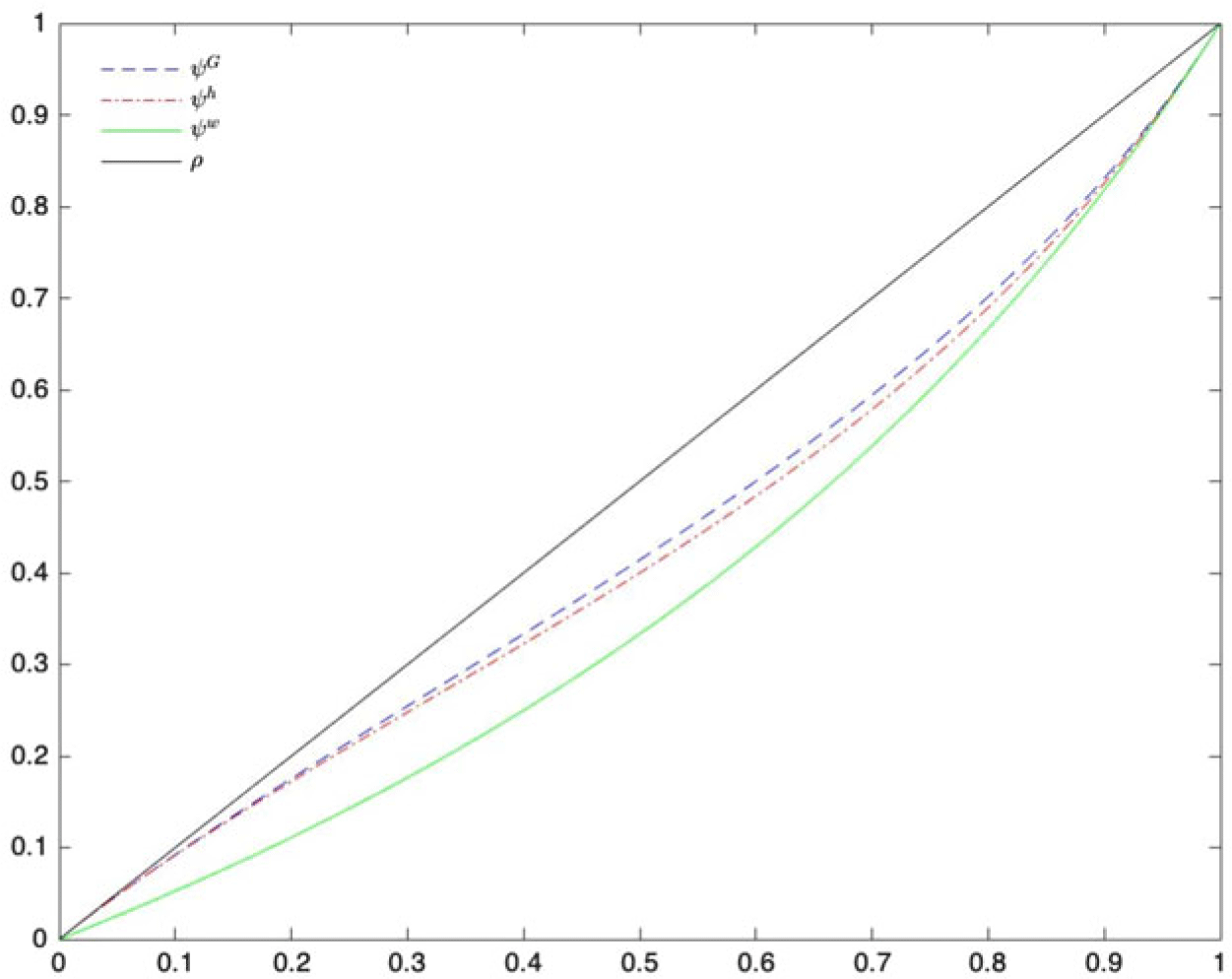
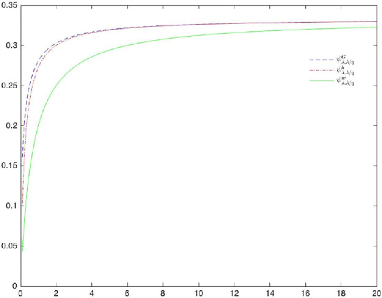
We will explain in the discussion why  $\rho> \psi^G > \psi^h > \psi^w$
, and this is confirmed graphically in Figure 1.
A plot of  $\psi^w$
,
 $\psi^h$
, and
 $\psi^G$
as functions of
 $\rho$
, as well as the line
 $y(\rho) = \rho$
. Note that for
 $g(x)=x$
we have
 $h^\lambda(x) = \rho x$
and
 $G^c(x) = \psi^c x$
.

First observe that as  ${\mathcal T}_\lambda \subset {\mathcal T}$
we must have
 $h^\lambda \leq w$
, and since
 $h^\lambda$
is optimal for stopping at event times of the Poisson process we must have
 $G^c < h^\lambda$
.
In the problem with a linear payoff it is always optimal to stop as soon as possible, both in the classical optimal stopping problem, and in the stopping problem in which stopping times are restricted to be event times of the Poisson process. This remains true in the randomised stopping problem, to the extent that the problem value is maximised if the probability of stopping is maximised. Since the probability of stopping  ${{g}/{(g+c)}}$
is maximised when c is minimised, it follows from the inequalities
 $G^c < h^\lambda < w$
that the value functions have order
 $G^G > G^h > G^w$
. Hence
 $\psi^G > \psi^h > \psi^w$
. Further, all these valuations are dominated by the case of optimal stopping where stopping times are constrained to be event times of the Poisson process, and so
 $\psi^G < \rho$
.
For all specifications of continuation value,  $\psi^c$
has limiting values
 \[\psi^c(0+)=0 \quad\text{and}\quad \psi^c(1-)=1.\]
When  $\lambda$
is very small,
 $T_1=T^\lambda_1$
is likely to be large,
 ${\mathrm{e}}^{-\beta T_1}{X_{T_1}}$
is small with large probability, and the value function is small. Conversely, if
 $\beta - \mu$
is small,
 ${\mathbb E}[{\mathrm{e}}^{-\beta T^\lambda_k}{X_{T^\lambda_k}}]$
is close to unity. Although the agent would benefit most from stopping at each and every opportunity, the losses from not stopping are not great.
Note that  $\psi^c$
is increasing in
 $\rho$
for each
 $c \in \{w,h,G\}$
. This corresponds to the value function being increasing in
 $\lambda$
. Consider first the case
 $c=w$
. As
 $\lambda$
increases, there are more chances to stop. Since w does not depend on
 $\lambda$
, the probability of stopping, conditional on an opportunity to stop, does not depend on
 $\lambda$
. Hence a simple coupling argument gives that as
 $\lambda$
increases the stopping time gets smaller and therefore the value function increases. Now consider the case
 $c=h$
. As
 $\lambda$
increases, there are more opportunities to stop. However,
 $h^\lambda$
is increasing in
 $\lambda$
, and so at each opportunity to stop the agent is less likely to stop. This second factor is less significant than the first, and overall the rate of stopping
 $\lambda \Gamma(x, h^\lambda (x))$
goes up. Hence
 $\psi^h$
is increasing in
 $\lambda$
. Finally suppose
 $c=G$
. Again, increasing
 $\lambda$
increases the stopping opportunities, which has the impact of increasing the value function. However, this reduces the probability of stopping, which has the effect of reducing the size of any increase in value function, but not to the extent of preventing overall increases.
5. Call payoffs
Our goal in this section is to move beyond linear payoffs to call payoffs. In particular we will assume  $g(x) = (x-K)^+$
. By a scaling argument it is possible to reduce the case of general strike to unit strike, and in all our numerical examples we will assume
 $K=1$
, but for the present we allow general K.
Standard arguments give an explicit formulae for w, namely
 \begin{equation*}w(x)=\begin{cases}\dfrac{L^*}{\theta} \biggl( \dfrac{x}{L^*} \biggr)^\theta & x
< L^* {,}\\ \\[-6pt] g(x) & x\geq L^*, \\\end{cases}\end{equation*}
where  $L^*= ({{\theta}/{(\theta-1)}}) K$
and
 $\theta>1$
is given by
 \begin{equation}\theta =\biggl(\dfrac{1}{2}-\dfrac{\mu}{\sigma^2} \biggr)+\sqrt{\biggl(\dfrac{1}{2}-\dfrac{\mu}{\sigma^2}\biggr)^2+\dfrac{2\beta}{\sigma^2}}.\end{equation}
We can solve for  $h^\lambda$
by noting that it is optimal to stop at
 $(t,X_t)$
if and only if there is an event of the Poisson process and
 $h(X_t)\leq (X_t-K)$
. We expect that there is a critical value
 $L^\lambda$
such that it is optimal to stop at
 $(t,X_t)$
if and only if
 $X_t>L^\lambda$
. Then we have
 ${\mathcal L} G = \beta G$
for
 $x \leq L^\lambda$
and
 ${\mathcal L} G -(\beta+\lambda) G + \lambda g(x)=0$
for
 $x \geq L^\lambda$
. We have value matching and smooth fit at
 $x=L^\lambda$
, and from the fact that
 $L^\lambda$
separates the stopping and continuation regions, we have
 $G(L^\lambda) =g(L^\lambda) = (L^\lambda - K)^+$
. We find
 \begin{equation}h^\lambda(x) = h(x)=\begin{cases}C x^{\theta} & x
< L^\lambda,\\ \rho x -\dfrac{\lambda K}{\lambda +\beta}+ C_1 x^{\gamma} & x\geq L^\lambda,\\\end{cases}\end{equation}
where
 \begin{equation*} \gamma=\biggl(\dfrac{1}{2}-\dfrac{\mu}{\sigma^2} \biggr)- \sqrt{\biggl(\dfrac{1}{2}-\dfrac{\mu}{\sigma^2}\biggr)^2+\dfrac{2(\beta+\lambda)}{\sigma^2}}\end{equation*}
(note that  $\gamma<0$
), and
 \begin{align*}L^\lambda & = \dfrac{\lambda+\beta - \mu}{\lambda+\beta} \dfrac{ \gamma }{\gamma-1} \dfrac{\theta }{\theta -1}K,\\[3pt] C & = \dfrac{\lambda}{\lambda+\beta} \dfrac{\gamma}{\gamma-\theta} \dfrac{1}{\theta-1} K (L^\lambda)^{-\theta}{,} \\[3pt] C_1 & = \dfrac{\lambda}{\lambda+\beta} \dfrac{\theta}{\gamma-\theta} \dfrac{1}{\gamma-1} K (L^\lambda)^{-\gamma}.\end{align*}
Note that  $\lim_{\lambda \uparrow \infty} \gamma = - \infty$
and thus
 $\lim_{\lambda \uparrow \infty} L^\lambda = L^*$
. Note further that
 \[\lim_{\lambda \uparrow \infty} C = \dfrac{1}{\theta-1} K (L^*)^{-\theta} = \dfrac{1}{\theta}(L^*)^{1-\theta}{,}\]
where we use  $L^* = ({{\theta}/{(\theta - 1)}}) K$
and similarly
 $\lim_{\lambda \uparrow \infty} C_1 = 0$
. Moreover,
 $C_1 x^\gamma \rightarrow 0$
for fixed x, and hence
 $\lim_{\lambda \uparrow \infty} h^\lambda(x) = w(x)$
.
5.1.
$\boldsymbol{c=w}$

The first randomised stopping problem we consider is for the case where the continuation value is the value of the problem with no restrictions on the exercise time.
Recall that  $L^* = ({{\theta}/{(\theta-1)}}) K$
. Then
 $G^w$
satisfies
 \begin{align}\mathcal{L}G^w - \beta G^w =0{,} \quad x \in (0,K), \end{align}
 \begin{align} \mathcal{L}G^w -(\beta + \lambda) G^w + \lambda \dfrac{g^2+ wG^w}{g+w}=0{,}\quad x\in[K,L^*), \end{align}
 \begin{align} \mathcal{L}G^w - \biggl(\beta + \dfrac{\lambda}{2}\biggr) G^w+ \dfrac{\lambda }{2} g=0{,}\quad x \in [L^*,\infty). \end{align}
Note that when  $g=0$
the ODE in (17) reduces to the ODE in (16), and so the first two cases might simply be combined. However, in describing the construction of the solution it is convenient to divide
 $(0,L^*)$
into two regions.
The general solution to (16) is
 \[G^w(x) = B_1 x^{\theta} + B_2 x^{\theta_2},\]
where  $\theta$
is given by (14) and
 $\theta_2<0$
is given by
 \begin{equation*} \theta_2=\biggl(\dfrac{1}{2}-\dfrac{\mu}{\sigma^2} \biggr)-\sqrt{\biggl(\dfrac{1}{2}-\dfrac{\mu}{\sigma^2}\biggr)^2+\dfrac{2\beta}{\sigma^2}} .\end{equation*}
From the boundary condition  $G^w(0+)=0$
we must have
 $B_2=0$
.
Similarly, the general solution to  $\mathcal{L}G - (\beta + {{\lambda}/{2}})G=0$
is given by
 $G(x) = B_3 x^{\alpha_+} + B_4 x^{\alpha_-}$
, where
 $\alpha_+>1$
and
 $\alpha_-<0$
are given by
 \[\alpha_{\pm}=\biggl(\dfrac{1}{2}-\dfrac{\mu}{\sigma^2} \biggr) \pm\sqrt{\biggl(\dfrac{1}{2}-\dfrac{\mu}{\sigma^2}\biggr)^2+\dfrac{2\beta+\lambda}{\sigma^2}}.\]
A particular solution to (18) is given by
 \[G(x) = \dfrac{\lambda}{\lambda + 2 \beta -2\mu} x -\dfrac{\lambda K}{\lambda + 2\beta}= \dfrac{\rho}{2-\rho} x -\dfrac{\lambda K}{\lambda +2 \beta}{.}\]
Since the solution  $G^w$
we want is of linear growth rate, we require
 $B_3=0$
, and it follows that, for
 $x \in (L^*,\infty)$
,
 \begin{equation}G^w(x) = \psi^w x -\dfrac{\lambda}{\lambda +2 \beta} K + B_4 x^{\alpha_-},\end{equation}
for a constant  $B_4$
to be determined.
The goal is to construct a  $C^2$
solution for
 $G=G^w$
on
 $(0,\infty)$
. Fix a solution for G on (0, K) by fixing
 $B_1$
. We can use value matching and smooth fit at K to give values for G and G’ at K and hence to construct a (numerical) solution to (17) on
 $[K,L^*)$
. Value matching at
 $L^*$
can be used to construct a solution to (18) on
 $(L^*,\infty)$
, and in particular to fix
 $B_4$
in (19). In general there will be no first-order smooth fit at
 $L^*$
. However, by adjusting
 $B_1$
we can construct a solution which is
 $C^1$
at K and
 $L^*$
and hence
 $C^1$
on
 $(0,\infty)$
. This is the solution we want.
Note that if we set  $g=0$
at
 $x=K$
then (17) reduces to (16), and if we set
 $g=w$
at
 $x=L^*$
then (17) reduces to (18). As a result, if we have a solution which is
 $C^1$
at K and
 $L^*$
, then the second derivatives also match at these points, and our
 $C^1$
solution is actually
 $C^2$
.
5.2.
$\boldsymbol{c=h}$

Now suppose we take as the continuation value the value of the game under optimal stopping when the stopping opportunities are the event times of a Poisson process, rate  $\lambda$
. We have that
 $G^h$
satisfies
 \begin{equation}\mathcal{L}G^h - (\beta + \lambda) G^h + \lambda \dfrac{g^2+ hG^h}{g+ h}=0 , \quad x\in (0, \infty),\end{equation}
where h is given by (15). Note that g changes form at K and  $h^\lambda$
changes form at
 $L^\lambda$
, so that (20) can usefully be split into three regions. As in the previous case, the boundary condition at
 $0+$
is such that the solution on (0,K] takes the form
 $G^h(x) = D x^{\theta}$
for some constant D. Temporarily fixing D, value matching and first-order smooth fit at K allows us to construct a solution on
 $[K,\infty)$
. We want the solution for which
 $\lim {{G^h(x)}/{x}} = \psi^h$
; we adjust D until this is the case. Again, since g and
 $h^\lambda$
are continuous at K and
 $L^\lambda$
, the
 $C^1$
solution from (20) is automatically
 $C^2$
.
5.3.
$\boldsymbol{c=G}$

We distinguish between the two regions for (11):
 \begin{align} \mathcal{L}G - \beta G =0, \quad x \in (0,K){,} \end{align}
 \begin{align} \mathcal{L}G - (\beta + \lambda) G + \lambda \dfrac{g^2+ G^2}{g+ G}=0 , x\in[K,\infty). \end{align}
The general solution to (21) on (0,K) is given by  $G(x)= E x^{\theta}$
for some constant E. Fixing E and using value matching and first-order smooth fit, we can construct (numerically) a
 $C^1$
solution for G on
 $(0,\infty)$
. Finally, we can adjust E until we obtain a solution with linear growth which satisfies
 $ \lim_{x \rightarrow \infty} ({{G(x)}/{x}}) = \psi^G$
.
5.4. Comparison of the different solutions
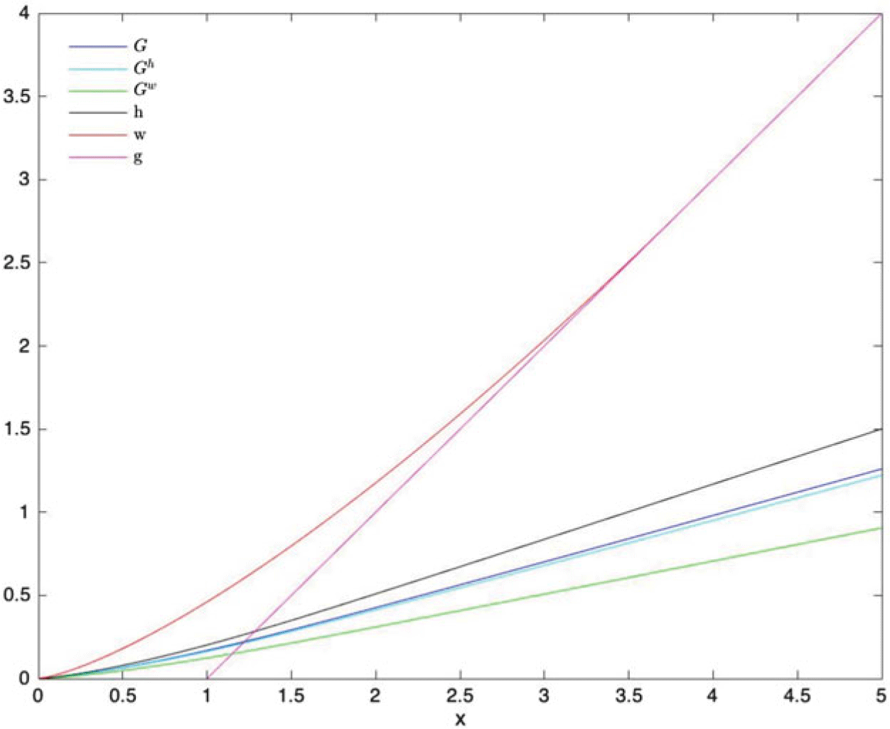
Figure 2 plots the various value functions w,  $h=h^\lambda$
,
 $G^w$
,
 $G^h$
, and
 $G^G$
together with the payoff
 $g(x)=(x-1)^+$
. Here w is the largest of the value functions, reflecting the fact that stopping is unrestricted and optimal. Next largest is h, which involves optimal stopping from the event times of the Poisson process: optimality means that
 $h \geq \max \{G^w, G^h, G^G\}$
.
The value functions depicted are based on the parameter set  $(\beta,\mu,\sigma,K,\lambda) =(5,3,2,1,1)$
; the curved lines are the value functions (g is piecewise linear) and
 $w>h>G^G> G^h>G^w$
always holds.

Since  $w>h$
, when we compare the stopping probability for randomised stopping under continuation value w compared with that of h, we expect to stop less frequently. In general, discounting means that above and not too close to the strike it is beneficial to stop sooner. Hence
 $G^h>G^w$
. (Below the strike
 $g\equiv 0$
, and the probability of stopping is zero. Just above the strike, stopping is more common for
 $c=h$
than for
 $c=w$
, and stopping is sub-optimal in this case; nonetheless, this regime is small and
 $G^h>G^w$
.)
Similar reasoning justifies why  $G^G<h$
leads to
 $G^G>G^h$
. From Figure 2 we see that
 $h-G \ll w-h$
, and from this we expect that
 $G^G-G^h \ll G^h- G^w$
, where by
 $\ll$
we mean much smaller than in a qualitative sense. Again the evidence from Figure 2 supports this conclusion.
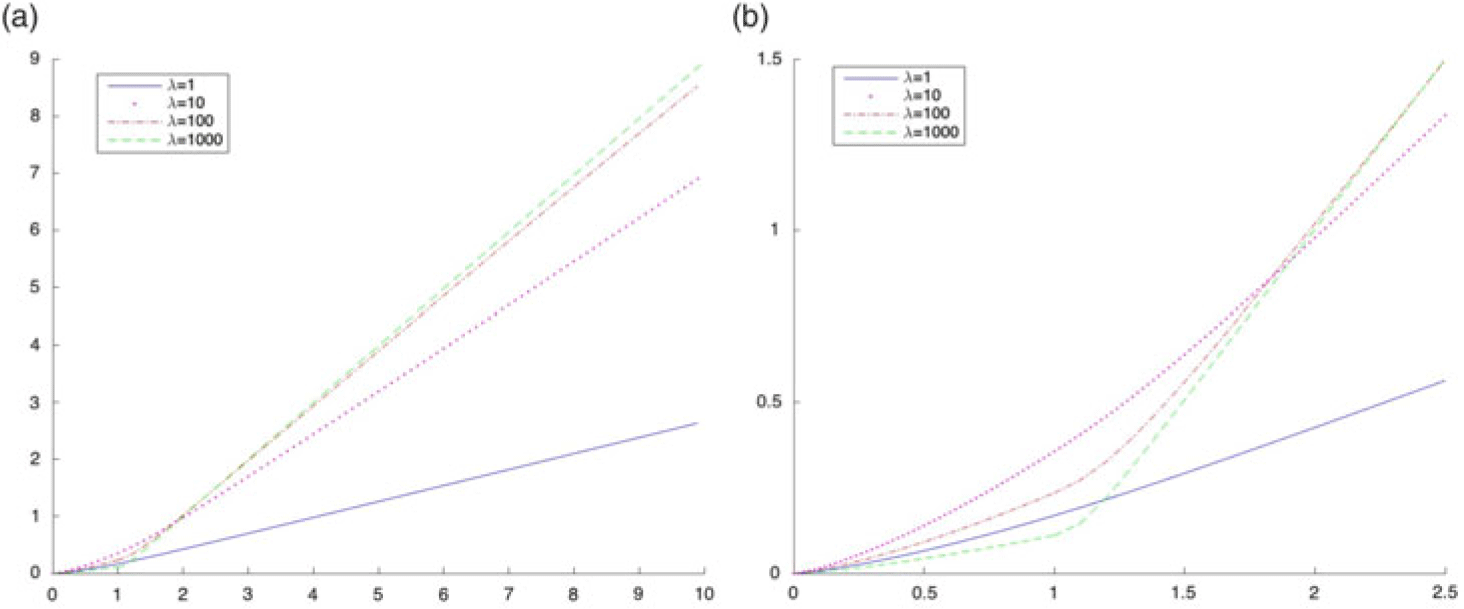
Figure 3 shows the impact of increased stopping opportunities and shows the value function as a function of x for various values of  $\lambda$
. Surprisingly, in general the value function is non-monotonic in
 $\lambda$
. For large values of x (see panel (a)) we have that
 $G^G(x)$
is monotonic in
 $\lambda$
: for large x it is always optimal to stop and hence more stopping opportunities are beneficial (recall that asymptotically
 ${{G^G(x)}/{x}} \rightarrow \psi^G$
and
 $\psi^G$
is monotonic in
 $\lambda$
: see Figure 1). However, this monotonicity does not propagate to all values of x. For x close to the strike (see panel (b)) the value function is non-monotonic. This reflects the multiple impacts of increasing
 $\lambda$
: it increases the stopping opportunities and hence also the rate of stopping, but near the strike, since stopping is worse than continuing, more stopping can reduce the value function. Overall, the impact of increasing the rate stopping opportunities is ambiguous.
Plot of the value functions when  $\lambda =1$
,
 $\lambda=10$
,
 $\lambda=100$
, and
 $\lambda=1000$
, respectively: (a)
 $G^G$
as a function of
 $\lambda$
; (b) close-up near
 $K=1$
. In (a) the value functions are seen to be increasing in
 $\lambda$
at least for large x. In (b) we see that this monotonicity does not hold for
 $\lambda$
near the strike. Other parameters are
 $(\beta,\mu,\sigma,K) = (5,3,2,1)$
.

6. Towards a model of continuous stopping
6.1. Modification of the randomising stopping rule
If we assume that the probability of stopping (conditional on an event of the Poisson process) is a constant  $p>0$
, independent of
 $X_t$
(which is the case when the payoff is linear or equivalently when the strike price K is 0), then the time of stopping is an exponentially distributed random variable with rate
 $p\lambda$
. Then, as opportunities to stop come faster and faster
 $(\lambda \rightarrow \infty)$
, the time of stopping converges to 0, almost surely. Without modification to our model, if stopping opportunities become more and more frequent, then in the limit the randomising stopping rule will be degenerate and will involve stopping immediately wherever
 $g>0$
.
In order to avoid this degenerate limit we consider biasing the continuation probability towards continuing: we modify the stopping probability (previously  $\Gamma(g,c) = {{g}/{(g+c)}}$
) to
 \[\Gamma_\xi = \Gamma_\xi(g,c) = \dfrac{g}{g+\xi c} .\]
As in Section 4, in the case of linear payoffs we can derive exact expressions for the value function: these take the form  $V^c_\xi(x) = \psi^c_{\lambda,\xi} x$
, where
 \begin{align}\psi^G_{\lambda,\xi} = - \dfrac{1}{2\xi(1-\rho)} + \sqrt{\dfrac{1}{4\xi^2(1-\rho)^2} + \dfrac{\rho}{\xi(1-\rho)}}, \end{align}
 \begin{equation} \hspace*{-115pt}\psi^h_{\lambda,\xi} = \dfrac{\rho}{1+\xi \rho - \xi \rho^2},\hfill \end{equation}
 \begin{equation} \hspace*{-125pt}\psi^w_{\lambda,\xi} = \dfrac{\rho}{1+\xi - \xi \rho }.\hfill\end{equation}
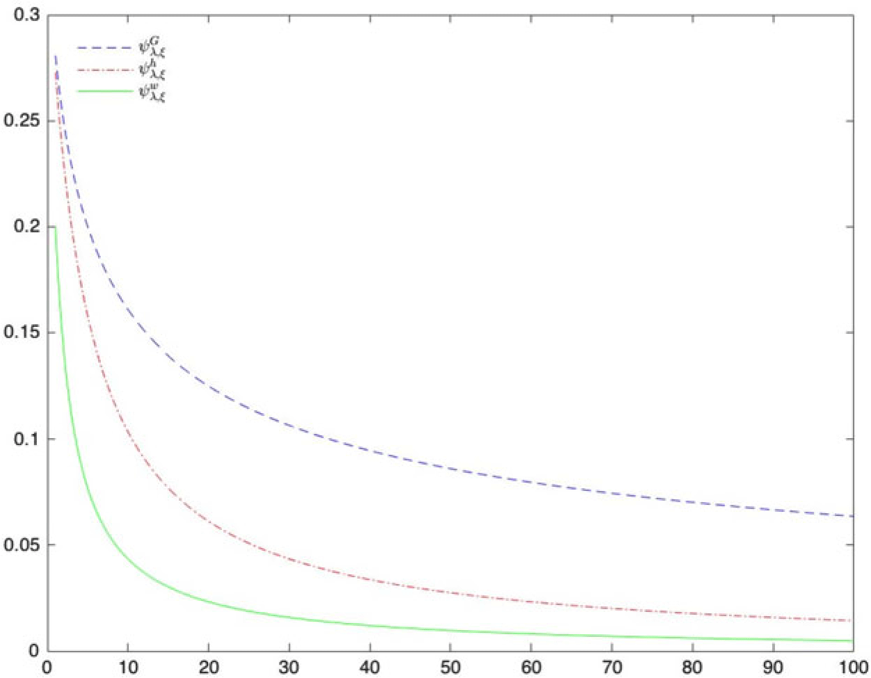
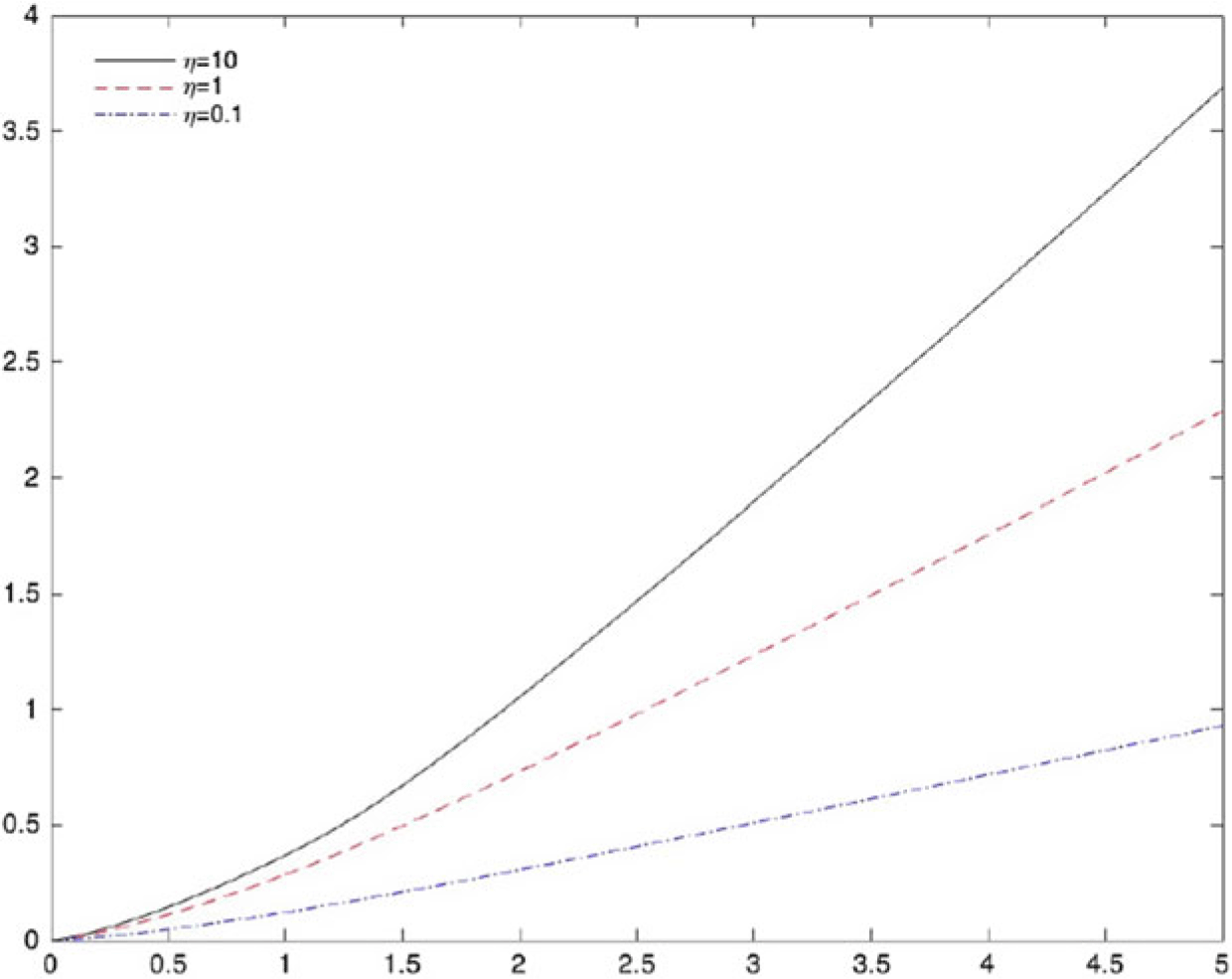
Figure 4 shows the impact of varying  $\xi$
. We can see that the values of linear payoffs are decreasing in
 $\xi$
. Increasing
 $\xi$
decreases the probability of stopping for all cases, and since stopping is optimal everywhere, discounting reduces the value of the payoff. Hence
 $\psi^c_{\lambda,\xi}$
is decreasing in
 $\xi$
for
 $c \in \{w,h,G \}$
. Moreover, since
 $G < h < w$
we find
 $\psi^G_{\lambda,\xi} > \psi^h_{\lambda,\xi} > \psi^w_{\lambda,\xi}$
.
 $(\beta,\mu,\sigma,\lambda) =(5,3,2,1)$
: plots of
 $\psi^G_{\lambda,\xi}$
,
 $\psi^h_{\lambda,\xi}$
, and
 $\psi^w_{\lambda,\xi}$
as functions of
 $\xi$
.

6.2. Making
$\xi$
dependent on
$\lambda$


Now we consider the impact of varying  $\lambda$
and
 $\xi$
in a systematic manner. Suppose
 $c(x)= \kappa g(x)$
for some constant
 $\kappa$
(for example, if
 $g(x)=x$
we find
 $c(x) = \kappa x$
for some
 $\kappa$
). Then
 $\Gamma_\xi(g,c) = {{1}/{(1 + \xi \kappa)}}$
is independent of x, and the rate of stopping is
 ${{\lambda}/{(1 + \kappa \xi)}}$
. We want to choose
 $\lambda \uparrow \infty$
,
 $\xi \uparrow \infty$
in such a way that the rate of stopping converges to a non-trivial rate. In particular, we want to choose
 $\xi = \xi(\lambda)$
such that
 $\lim_{\lambda \uparrow \infty} {{\lambda}/{(1 + \kappa \xi(\lambda))}}$
exists in
 $(0,\infty)$
. Then, as opportunities to stop (from the Poisson process) become universal, the probability of stopping (in a fixed and finite time interval
 $[0,T_\epsilon]$
) converges to a probability in (0, 1).
Motivated by this heuristic, we take  $\xi = {{\lambda}/{\eta}}$
for
 $\eta \in (0,\infty)$
. Then
 \[\lambda \Gamma(g,c) = \dfrac{\eta \lambda g}{\eta g + \lambda c}.\]
In Figure 5 we plot  $\psi^c_{\lambda, {\lambda}/{\eta}}$
as a function of
 $\eta$
for
 $c \in \{w,h,G \}$
. We see that as
 $\eta$
increases
 $\psi^c_{\lambda,\lambda/\eta}$
increases. Moreover,
 $\psi^G_{\lambda,\lambda/\eta} > \psi^h_{\lambda,\lambda/\eta} > \psi^w_{\lambda,\lambda/\eta}$
, and the first two are almost indistinguishable for even moderately large values of
 $\eta$
.
 $\psi^c_{\lambda,\lambda/\eta}$
as a function of
 $\eta$
;
 $(\beta,\mu,\sigma,\lambda) =(5,3,2,1)$
.

Our main interest is in fixing  $\eta$
and letting both
 $\lambda$
and
 $\xi = {{\lambda}/{\eta}}$
get large. The values of
 $\psi^c$
are plotted as functions of
 $\lambda$
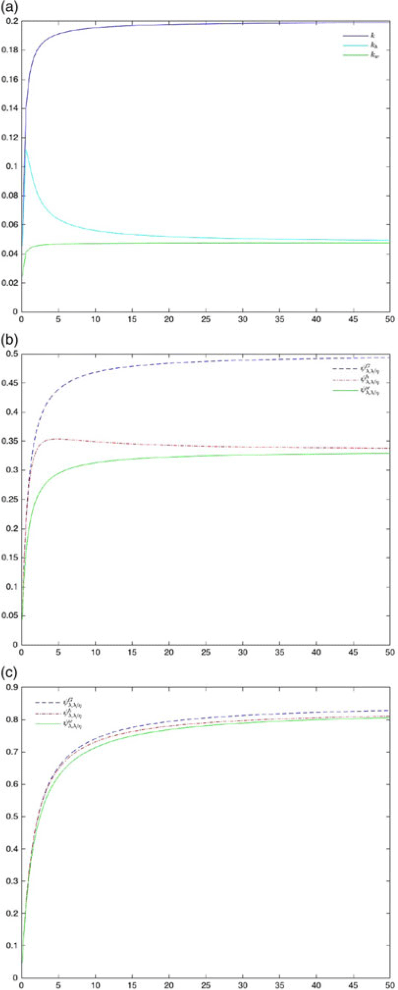
in Figure 6. Again we see
 $\psi^G_{\lambda,\lambda/\eta} > \psi^h_{\lambda,\lambda/\eta} > \psi^w_{\lambda,\lambda/\eta}$
. We also have that
 $\psi^h_{\lambda, {\lambda}/{\eta}}$
and
 $\psi^w_{\lambda, {\lambda}/{\eta}}$
converge to the same limit. This is because as
 $\lambda$
increases to infinity
 $h^\lambda$
converges to w, and so the continuation value is the same for these two specifications. However, this is a limiting result, and when
 $\lambda$
is small or moderate,
 $\psi^h_{\lambda,\lambda/\eta}$
is closer to
 $\psi^G_{\lambda,\lambda/\eta}$
than
 $\psi^w_{\lambda,\lambda/\eta}$
, recovering the result of Section 5.4.
(a)  $\psi^G_{\lambda,\lambda/\eta}(\lambda)$
,
 $\eta=01$
; (b)
 $\psi^G_{\lambda,\lambda/\eta}(\lambda)$
,
 $\eta=1$
; (c)
 $\psi^G_{\lambda,\lambda/\eta}(\lambda)$
,
 $\eta=10$
. Under the new randomising stopping rule
 $\Gamma_\xi$
for
 $\xi = \lambda/\eta$
, letting
 $\lambda$
get large (for fixed
 $\eta$
) does not lead to the degenerate case of stopping immediately. Instead we find
 $\lim_{\lambda \uparrow \infty} \psi^G_{\lambda,\lambda/\eta} < 1$
, corresponding to the fact that in the limit stopping occurs at a finite rate.

Recall the definitions of  $\psi^c_{\lambda,\xi}$
in (23)–(25) and consider
 $\lim_{\lambda \uparrow \infty} \psi^c_{\lambda,{\lambda}/{\eta}}$
. Define
 \begin{align}k^*_w = \lim_{\lambda \uparrow \infty} \psi^w_{\lambda,{\lambda}/{\eta}} & = \dfrac{\eta}{\eta+\beta-\mu}{,} \end{align}
 \begin{align}k^*_h = \lim_{\lambda \uparrow \infty} \psi^h_{\lambda,{\lambda}/{\eta}} & = \dfrac{\eta}{\eta+\beta-\mu}{,} \end{align}
 \begin{align}k^*_G = \lim_{\lambda \uparrow \infty} \psi^G_{\lambda,{\lambda}/{\eta}} & = -\dfrac{\eta}{2(\beta-\mu)} + \sqrt{\dfrac{\eta^2}{4(\beta-\mu)^2}+ \dfrac{\eta}{\beta-\mu}}{.}\end{align}
Then  $k^*_c$
describes the value function (in the limit of large
 $\lambda$
) for linear payoffs in the sense that for
 $g(x)=x$
,
 $\lim_{\lambda \uparrow \infty} V^c_{\lambda, \lambda/\eta}(x) = k^*_c x$
. By letting
 $\lambda$
and
 $\xi$
tend to infinity simultaneously we have obtained a non-degenerate limit. The limiting case
 $\lambda=\infty$
corresponds to a continuous flow of stopping opportunities, but with a non-trivial probability of stopping in each fixed interval [0,T]. In particular,
 $G^\lambda = G^{\lambda,\xi = \lambda/\eta,c}$
solves
 \[0 = \{ {\mathcal L} G^\lambda - \beta G^\lambda + \lambda \Gamma_{\lambda/\eta} (g,c) (g-G^\lambda) \} = {\mathcal L} G^\lambda - \beta G^\lambda + \lambda \dfrac{\eta g (g-G^\lambda)}{\eta g+\lambda c}.\]
Assuming  $G^c_\eta = \lim_{\lambda \uparrow \infty} G^{\lambda,\xi = \lambda/\eta,c}$
exists and that we can swap the order of taking limits and differentiation, we obtain that
 $G^c_\eta$
solves
 \begin{equation} {\mathcal L} G^c_\eta - \beta G^c_\eta + \eta \dfrac{g}{c} ( {g} - {G^c_\eta} ) = 0.\end{equation}
For the case where the strike price is 0 (i.e.  $g(x)=x$
), the above ODE can be solved analytically and the solution is given by
 $G^c_\eta (x) = k_c^* x$
with
 $k_c^* $
given by (26)–(28).
6.3. Alternative formulation of the limiting case
In this section we propose a problem in continuous time in which the value function solves the same equation as that derived in the previous section, and hence represents a candidate continuous-time randomised stopping problem.
Suppose stopping opportunities occur as events of a time-inhomogeneous Poisson process with rate  $\Lambda^c_\eta=\Lambda^c_\eta(x)$
, where
 \begin{equation*} {\Lambda}^c_\eta (x)= \dfrac{ \eta g(x)}{c(x)}{,} \end{equation*}
and that the option is exercised at every stopping opportunity. Here, as always, c is the continuation value, and in this model the rate of stopping depends on the ratio of the instantaneous payoff to the continuation value. Note that we identify stopping opportunities via an inhomogeneous Poisson process rather than by thinning a homogeneous Poisson process of rate  $\lambda$
, hence it makes sense to consider
 $c \in \{w,G\}$
but not
 $c=h^\lambda$
.
The expected discounted reward from stopping can be represented via the stochastic formulation
 \begin{equation}G^c_\eta(x) = {\mathbb E}^x \biggl[ \int^\infty_0 \Lambda^c_\eta(X_t) {\mathrm{e}}^{- \int^t_0 \Lambda^c_\eta(X_s)\,{\mathrm{d}} s} {\mathrm{e}}^{-\beta t} g(X_t) \,{\mathrm{d}} t \biggr].\end{equation}
By analogy with the results in the previous section we assume that (30) has a unique solution, and that this solution is the unique solution of linear growth to the ordinary differential equation
 \begin{equation} {\mathcal L} G(x)- [ \beta + \Lambda(x)] G(x ) + {\Lambda}(x)g(x) =0.\end{equation}
Substituting for  ${\Lambda}$
in (31) we find that G solves (29). (This justifies why we have used the same notation
 $G=G^c_\eta$
for the value function in both Section 6.2 and this section.) Thus we have another interpretation for the continuous case
 $(\lambda \rightarrow \infty)$
under the biased randomising stopping rule
 $\Gamma_{\xi = \lambda/\eta}$
. This agent is employing a strategy of stopping at the first event time of an inhomogeneous Poisson process with rate
 \[\Lambda^c_\eta(X_t)=\dfrac{\eta g(X_t)}{c(X_t)}.\]
6.3.1. Linear payoffs
If  $g(x)=x$
then it is always optimal to exercise immediately and
 $w(x)=x$
. Then, in the case
 $c=w$
it follows from trying the candidate
 $G(x)=kx$
in (31) that
 $G^w_\eta(x) = k^*_w x$
, where
 $k^*_w$
is given by (26). Similarly, in the case
 $c=G$
we find
 $G^G_\eta(x) = k^*_G x$
, where
 $k^*_G$
is given by (28).
Since  $G^G_\eta(x) < w(x)$
we find
 $\Lambda^G_\eta(\!\cdot\!) > \Lambda^w_\eta(\!\cdot\!)$
, and hence when the continuation value is given by G we stop sooner than when the continuation value is given by w. This explains why
 $G^G > G^w$
, or equivalently
 $k^*_G > k^*_w$
.
6.3.2. Call payoffs
Now we suppose  $g(x)=(x-1)^+$
and consider numerical solutions of (31). The solutions
 $G^G_\eta$
and
 $G^w_\eta$
are increasing and convex in x and satisfy
 \[\lim_{x \rightarrow \infty} \dfrac{G^c_\eta(x)}{x} = k^*_c.\]
Furthermore (see Figure 7),  $G^G_\eta$
is increasing in
 $\eta$
. This is because, certainly when x is large, it is advantageous to stop, and the stopping rate increases as
 $\eta$
increases. The picture for
 $G^w$
as a function of
 $\eta$
is very similar.
 $(\beta,\mu,\sigma) =(5,3,2)$
.
 $G^G_\eta$
as a function of
 $\eta$
. We see that
 $G^G_\eta$
is increasing in
 $\eta$
. We find a similar picture for
 $G^w_\eta$
.

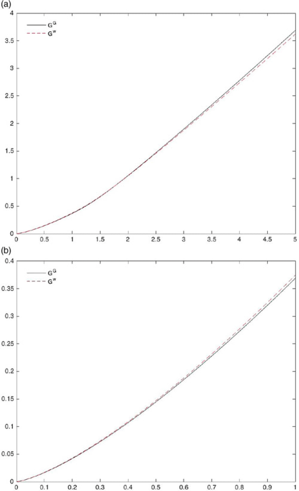
In Figure 8 we compare  $G^G_\eta$
with
 $G^w_\eta$
. When
 $\eta = 0.1$
or
 $\eta = 1.0$
we find
 $G^G(x)>G^w(x)$
for all values of x. However, when
 $\eta = 10$
there is no universal relationship between
 $G^G_\eta$
and
 $G^w_\eta$
. We still find that
 $G^G_\eta(x)>G^w_\eta(x)$
for large x, but for small x the inequality is reversed. As we have found elsewhere, the feedback element implicit in the definition of
 $G^G$
means that an increased value function increases the stopping rate, which can lower the value function in the region where g is small and stopping is not beneficial.
 $(\beta,\mu,\sigma) =(5,3,2)$
. A comparison of the value functions
 $G^G_\eta$
and
 $G^w_\eta$
when
 $\eta = 10$
. Over most of the range we find
 $G^G_\eta>G^w_\eta$
, and this is true in the limit of large x. However, for small x (see panel (b), which focuses on small x), we find that
 $G^G_\eta < G^w_\eta$
.

Appendix A. Proof of Theorem 1
We prove Theorem 1 via a series of auxiliary results. In particular, we show the following.
• If
$f^{\mathrm{STF}}$
is the solution of the stopping time formulation then
$f^{\mathrm{STF}}$
solves (10).• If
$f^{\mathrm{SFF}}$
is of polynomial growth and solves (10) then it also solves (11).• If
$f^{\mathrm{ODEF}}$
is of linear growth and solves (11) then it also solves (10).• There is a unique solution to the SFF problem.


When  $c=w$
or
 $c=h$
it is clear that there is a unique solution under the stopping time formulation, and in those cases Theorem 1 follows immediately from these results. When
 $c=G$
, in order to complete the proof of Theorem 1 we need an additional result (Lemma A.2) to say that a solution of Problem 2 also solves Problem 1.
Proof. As discussed at the start of Section 3, since the payoff function is bounded by a linear function, so are w,  $h^\lambda$
, and the solution to Problem 1. Let
 ${{\mathcal T}}^\lambda_t$
be the set of stopping times taking values in the event times of the Poisson process which are greater than t, and let
 $\hat{{\mathcal T}}^\lambda_t$
be the set of stopping times taking values in the union of
 $\{t\}$
and the event times of the Poisson process which are greater than t. (Then, for example, a stopping time
 $\sigma \in \hat{{\mathcal T}}^\lambda_0$
can either take the value 0 or the event time of the Poisson process.) Allowing stopping times in
 $\hat{{\mathcal T}}^\lambda_0$
is equivalent to allowing immediate exercise.
Then, conditioning on the first event time  $T_1$
of the Poisson process and using the strong Markov property,
 \begin{align*}G^c(x) & = {\mathbb E}^x \biggl[ \int_0^\infty {\mathrm{d}} t \lambda {\mathrm{e}}^{-\lambda t} {\mathbb E}^x[ {\mathrm{e}}^{-\beta \tau_G }g(X_{\tau_G}) \mid T_1=t, X_t ] \biggr] \\[2pt] & = \int_0^\infty {\mathrm{d}} t \lambda {\mathrm{e}}^{-(\beta+\lambda) t} {\mathbb E}^x \Bigl[ \Gamma(g(X_t),c(X_t)) g(X_t) \\[2pt] &
\quad\, + ( 1 - \Gamma(g(X_t),c(X_t)) ) {\mathbb E}^{X_t}\big[ {\mathrm{e}}^{-\beta (\tau_G-t)}g(X_{\tau_G})\mid \tau_G>t\big] \Bigr] \\[2pt] & = \int_0^\infty {\mathrm{d}} t \lambda {\mathrm{e}}^{-(\beta+\lambda)t} {\mathbb E}^x [ \Gamma(g(X_t),c(X_t)) g(X_t) + ( 1 - \Gamma(g(X_t),c(X_t)) ) G^c(X_t) ] .\end{align*}
Finally, note that we can write  $X_t = xX^{(1)}_t$
, where
 $X^{(1)}$
is exponential Brownian motion with drift
 $\mu$
, volatility
 $\sigma$
, and initial value
 $X^{(1)}_0=1$
. It follows from dominated convergence and the continuity of g that
 $G^c(0)=0$
.
Recall that
 \[N= \min \{ n \colon U_n \leq \Gamma(g(X_{T^\lambda_n}),c(X_{T^\lambda_n})) \}\quad\text{and}\quad \tau_{G^c} = T^\lambda_N.\]
By hypothesis we have that  $f= G^c$
solves
 \begin{align*}f(x) & = {\mathbb E}^x \biggl[ \int_0^\infty {\mathrm{d}} t \lambda {\mathrm{e}}^{-(\beta + \lambda)t} \{ \Gamma(g(X_t),c(X_t)) g(X_t) + (1- \Gamma(g(X_t),c(X_t)))f(X_t) \} \biggr] \\[2pt]
& = {\mathbb E}^x \Big[ {\mathrm{e}}^{-\beta {T^\lambda_1}} \Big\{ \Gamma\big(g\big(X_{T^\lambda_1}\big),c\big(X_{T^\lambda_1}\big)\big) g\big(X_{T^\lambda_1}\big) + \big(1- \Gamma\big(g\big(X_{T^\lambda_1}\big),c\big(X_{T^\lambda_1}\big)\big)\big)f\big(X_{T^\lambda_1}\big) \Big\} \Big] \\[2pt]
&= {\mathbb E}^x \Big[ {\mathrm{e}}^{-\beta {T^\lambda_1}} \Big\{ {\mathbb P}\big(U_1 \leq \Gamma\big(g\big(X_{T^\lambda_1}\big),c\big(X_{T^\lambda_1}\big)\big) g\big(X_{T^\lambda_1}\big)\big) \\[2pt] &
\quad\, + {\mathbb P}\big(U_1 > \Gamma\big(g\big(X_{T^\lambda_1}\big),c\big(X_{T^\lambda_1}\big)\big)\big)f\big(X_{T^\lambda_1}\big) \Big\} \Big] \\[2pt]
& = {\mathbb E}^x \Big[ {\mathrm{e}}^{-\beta {T^\lambda_1}} \Big\{ I_{\{ N=1 \} } g\big(X_{T^\lambda_1}\big) + I_{ \{ N>1 \} }f\big(X_{T^\lambda_1}\big) \Big\} \Big].\end{align*}
Similarly, on  $N>n$
,
 \[ f\big(X_{T^\lambda_{n}}\big) = {\mathbb E} \Big[ {\mathrm{e}}^{-\beta \big(T^\lambda_{n+1} - {T^\lambda_n}\big)} \Big\{ I_{\{ N=n+1 \} } g\big(X_{T^\lambda_{n+1}}\big) + I_{ \{ N>n+1 \} }f\big(X_{T^\lambda_{n+1}}\big) \Big\} \mid {\mathcal F}_{T^\lambda_{n}} \Big]. \]
Hence
 \[ f(x) = {\mathbb E}^x \Biggl[ \sum_{k=1}^n {\mathrm{e}}^{-\beta {T^\lambda_k}} I_{\{ N=k \} } g\big(X_{T^\lambda_k}\big) + {\mathrm{e}}^{-\beta T^\lambda_n} I_{ \{ N>n \} }f\big(X_{T^\lambda_n}\big) \Biggr] . \]
Letting n tend to infinity and using that f is of linear growth and 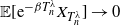 ${\mathbb E}[{\mathrm{e}}^{-\beta T^\lambda_n}X_{T^\lambda_n}] \rightarrow 0$
, we have
 \begin{align*} \hspace*{24pt} f(x) = {\mathbb E}^x \Biggl[ \sum_{k=1}^\infty {\mathrm{e}}^{-\beta {T^\lambda_k}} I_{\{ N=k \} } g\big(X_{T^\lambda_k}\big) \Biggr] ={\mathbb E}^x \Big[ {\mathrm{e}}^{-\beta T^\lambda_{N}} g\big(X_{T^\lambda_{N}}\big)\Big] = {\mathbb E}^x \big[ {\mathrm{e}}^{-\beta \tau_{G^c}} g(X_{\tau_{G^c}})\big]. \hspace*{28pt}\Box\end{align*}


Proof. It is a classical result (see e.g. Petrovski [Reference Petrovski13, Chapter 3.18] or Karatzas and Shreve [Reference Karatzas and Shreve8, page 254]) that if  $F\colon {\mathbb R}_+ \rightarrow {\mathbb R}_+$
is Borel-measurable and satisfies
 \[\int_0^\infty {\mathrm{e}}^{-a(\ln x)^2} F(x) d(\ln x)
< \infty\quad\text{for some $a>0$,}\]
then  $u^F$
is
 $C^\infty$
, where
 $u^F(t,x)$
is defined by
 \[u^F(t,x) = {\mathbb E}^x[F(X_t)] =\int^\infty_0 F(y) P(t; x,y) \,{\mathrm{d}} y\]
and  $P(t;x,y)$
is the transition density of a geometric Brownian motion.
Recall that  $G=G^c$
is of linear growth. Then
 $V=V^c$
, which is the weighted average of two functions of linear growth, is also of linear growth. In particular,
 $u^{V}$
is
 $C^\infty$
. Then
 \[ G(x) = {\mathbb E}^x \biggl[ \int^\infty_0 {\mathrm{e}}^{-\beta t} \lambda {\mathrm{e}}^{-\lambda t} V(X_t) \,{\mathrm{d}} t \biggr] = \int^\infty_0 \lambda {\mathrm{e}}^{-(\beta + \lambda) t} u^{V}(t,x) \,{\mathrm{d}} t\]
is also  $C^\infty$
. Furthermore, we can obtain bounds on the derivatives of G (see e.g. the proof of Problem 4.3.1 in Karatzas and Shreve [Reference Karatzas and Shreve8, page 277]) and it follows that, for example,
 \[ {\mathbb E}^x[X |G'(X)|] + {\mathbb E}^x[ X^2 | G''(X) |]
< C_0 + C_1 x. \]
Now we show that G solves (11). We follow Pham [Reference Pham14, page 43]. For  $\delta > 0$
, writing
 $t=s+\delta$
, we have
 \begin{align} G(x) & ={\mathbb E}^x \biggl[ \int^\delta_{t=0} \lambda {\mathrm{e}}^{-(\beta+\lambda) t} V(X_t) \,{\mathrm{d}} t \biggr] + {\mathbb E}^x \biggl[ {\mathbb E} \biggl[ \int_{s=0} ^\infty \lambda {\mathrm{e}}^{- (\beta+\lambda) (s+\delta)} V(X_{s+\delta}) \,{\mathrm{d}} s \mid {\mathcal F}_{\delta} \biggr] \biggr] \notag \\[2pt] & ={\mathbb E}^x \biggl[ \int^\delta _0 \lambda {\mathrm{e}}^{-(\beta+\lambda) t} V(X_t) \,{\mathrm{d}} t \biggr] + {\mathbb E}^x [ {\mathrm{e}}^{- (\beta+\lambda) \delta} G(X_\delta) ] .\end{align}
Let
 \[\tau_n = \inf \biggl\{ u\colon X_u \notin \biggl( \dfrac{x}{n}, nx \biggr) \biggr\}.\]
Since G is of class  $C^\infty$
, we apply Itô’s formula to
 ${\mathrm{e}}^{- (\beta+\lambda) t } G(X_t) $
to obtain
 \begin{align*}& {\mathrm{e}}^{- (\beta+\lambda) (\delta \wedge \tau_n)} G(X_{\delta\wedge \tau_n}) \\* & \quad = G(x) + \int^{\delta \wedge \tau_n}_0 {\mathrm{e}}^{- (\beta+\lambda)s} [{\mathcal L} G - (\beta + \lambda) G](X_s) \,{\mathrm{d}} s + \int^{\delta \wedge \tau_n}_0 {\mathrm{e}}^{- (\beta+\lambda)s} \sigma X_s G'(X_s) \,{\mathrm{d}} W_s \end{align*}
and hence
 \[ {\mathbb E}^x [ {\mathrm{e}}^{- (\beta+\lambda) (\delta \wedge \tau_n) } G(X_{\delta \wedge \tau_n}) ] = G(x) + {\mathbb E}^x \biggl[ \int^{\delta \wedge \tau_n}_0 {\mathrm{e}}^{- (\beta+\lambda)s} [{\mathcal L} G - (\beta + \lambda) G](X_s) \,{\mathrm{d}} s \biggr] . \]
Letting n tend to infinity and using the bounds on  ${\mathbb E}^x[X |G'(X)|]$
and
 ${\mathbb E}^x[ X^2 | G''(X) |]$
, by dominated and monotone convergence,
 \[ {\mathbb E}^x [ {\mathrm{e}}^{- (\beta+\lambda) \delta} G(X_{\delta}) ] = G(x) + {\mathbb E}^x \biggl[ \int^{\delta}_0 {\mathrm{e}}^{- (\beta+\lambda)s} [{\mathcal L} G - (\beta + \lambda) G](X_s) \,{\mathrm{d}} s \biggr] . \]
Plugging the above equation back into (A1), we get
 \[ G(x) = {\mathbb E}^x \biggl[ \int^\delta _0 \lambda {\mathrm{e}}^{-(\beta+\lambda) t} V(X_t) \,{\mathrm{d}} t + G(x) + \int^\delta_0 {\mathrm{e}}^{- (\beta+\lambda)s} [{\mathcal L} G - (\beta + \lambda) G](X_s) \,{\mathrm{d}} s \biggr] \]
and it follows that
 \begin{equation} 0 = {\mathbb E}^x \biggl[ \int^\delta_0 {\mathrm{e}}^{- (\beta+\lambda)s} [{\mathcal L} G - (\beta + \lambda) G + \lambda V ](X_s) \,{\mathrm{d}} s \biggr] .\end{equation}
Let
 \[J(s) = {\mathbb E}^x[ {\mathrm{e}}^{- (\beta+\lambda)s} \{ {\mathcal L} G - (\beta + \lambda) G + \lambda V \}(X_s)]\]
and note that J is continuous on  $[0,\infty)$
. Dividing both sides of (A2) by
 $\delta$
and sending
 $\delta$
to 0, we conclude from the mean-value theorem that there exists
 $\delta_n \downarrow 0$
such that
 $J(\delta_n)=0$
. Then, by continuity of J we conclude
 $J(0)=0$
, or equivalently
 $ {\mathcal L} G - (\beta + \lambda) G + \lambda V = 0. $
Setting
 $V = \Gamma(g,c)g + (1 - \Gamma(g,c))G$
, we find
 ${\mathcal L} G - \beta G + \lambda \Gamma(g,c) (g-G) = 0$
.
Lemma A.4. Suppose  $f=f(x,h)$
is continuous and of at most linear growth, suppose
 $\epsilon > \mu$
, and consider the ODE
 \begin{equation} {\mathcal L} H(x)- \epsilon H(x) + f(x,H(x)) =0.\end{equation}
Suppose H is a solution to (A3) of at most linear growth. Then H has the probabilistic representation
 \begin{equation} H(x) = {\mathbb E}^x \biggl[\int^\infty_0 {\mathrm{e}}^{-\epsilon t} f(X_t, H(X_t)) \,{\mathrm{d}} t \biggr] .\end{equation}
Proof. We have
 \[ H'' = \dfrac{2}{\sigma^2 x^2} \{ - \mu x H' + \epsilon H - f(x,H) \} \]
so that H is  $C^2$
. Then, applying Itô’s formula to
 ${\mathrm{e}}^{-\epsilon t} H(X_t)$
, we have
 \begin{align*}& {\mathrm{e}}^{-\epsilon ( t \land \tau_n )} H(X_{t \land \tau_n}) = H(x) + \int^{t \land \tau_n}_0 {\mathrm{e}}^{-\epsilon s} [{\mathcal L} H(X_s) - \epsilon H(X_s) ] \,{\mathrm{d}} s + \int^{t \land \tau_n}_0 {\mathrm{e}}^{-\epsilon s} H'(X_s) \sigma X_s \,{\mathrm{d}} W_s {,} \end{align*}
where, as before,
 \[\tau_n := \inf \biggl\{ u>0\colon X_u \notin \biggl(\dfrac{x}{n}, nx\biggr)\biggr\}.\]
Since the stopped stochastic integral is a martingale, taking expectations on both sides and using (A3), we get
 \begin{equation*}{\mathbb E}^x [ {\mathrm{e}}^{-\epsilon ( t \land \tau_n )} H(X_{t \land \tau_n}) ] = H(x) - {\mathbb E}^x \biggl[ \int^{t \land \tau_n}_0 {\mathrm{e}}^{-\epsilon s} f(X_s,H(X_s)) \,{\mathrm{d}} s \biggr] {.}\end{equation*}
Using the properties of exponential Brownian motion to conclude that  ${\mathbb E}^x[ \sup_{s \leq t} X_s ]< Cx$
for some C, sending n to infinity, and using dominated convergence and the assumed linear growth of H,
 \begin{equation*}{\mathbb E}^x [ {\mathrm{e}}^{-\epsilon t } H(X_{t}) ] = H(x) - {\mathbb E}^x \biggl[ \int^{t}_0 {\mathrm{e}}^{-\epsilon s} f(X_s,H(X_s)) \,{\mathrm{d}} s \biggr] .\end{equation*}
Then, since H is of linear growth and  $\epsilon > \mu$
, sending t to infinity we conclude
 \begin{align*}0 = \underset{t \rightarrow \infty }{\lim} {\mathbb E}^x [ {\mathrm{e}}^{-\epsilon t } H(X_{t}) ] & = H(x) - \underset{t \rightarrow \infty }{\lim}{\mathbb E}^x \biggl[ \int^{t}_0 {\mathrm{e}}^{-\epsilon s} f(X_s,H(X_s) \,{\mathrm{d}} s \biggr] \\[3pt]& = H(x) - {\mathbb E}^x \biggl[ \int^{\infty }_0 {\mathrm{e}}^{-\epsilon s} f(X_s,H(X_s)) \,{\mathrm{d}} s \biggr]. \end{align*}
Thus H admits probabilistic representation (A4).
Now, taking  $\epsilon = \lambda+ \beta$
,
 $H=G^c$
, and
 \[f(x,h)= \lambda \Upsilon^c(g(x),c(x),h) = \lambda \{ \Gamma(g(x),c(x))g(x) + (1-\Gamma(g(x),c(x))h \} {,}\]
we conclude
 \[G^c(x) = {\mathbb E}^x \biggl[ \int_0^\infty \lambda {\mathrm{e}}^{-(\lambda+\beta)t} \Upsilon^c(g(X_t), c(X_t), G^c(X_t)) \,{\mathrm{d}} t \biggr].\]
Proposition A.1. Suppose  $c \in \{ w, h^\lambda\}$
or
 $c=G$
and
 $\Gamma$
satisfies Hypothesis 1. Then there exists a unique
 $G=G^c$
which has the probabilistic representation (10), is of class
 $\mathcal{C}^2$
, and satisfies a linear growth condition.
Proof. Let (M,d) denote the metric space
 \begin{align*}M & = \{ f \colon (0,\infty) \mapsto (0,\infty), f \in C^2, 0< f(x)
< \kappa x\ \mbox{for some}\ \kappa \in {\mathbb R}_+\}, \\[3pt]d(H_1,H_2) & = \underset{x \in (0,\infty)}{\sup} \biggl| \dfrac{H_1(x)-H_2(x)}{x} \biggr|.\end{align*}
For c a perceived continuation value, define  $T^c\colon M \mapsto M$
by
 \[ T^c(F)(x) = {\mathbb E}^x\biggl[ \int^\infty_0 {\mathrm{e}}^{-(\beta+\lambda)t} \lambda ( \Gamma(g(X_t), c(X_t))g(X_t) + [1-\Gamma(g(X_t), c(X_t))]F(X_t) ) \,{\mathrm{d}} t \biggr].\]
To see that  $T^c(F) \in M$
, note first that
 $T^c(F)>0$
and
 $T^c(F)$
is of class
 $\mathcal{C}^2$
by Lemma A.3. Second, since g and F are of linear growth and
 $0 \leq \Gamma(g,c)g + (1 - \Gamma(g,c))F \leq {g+F}$
,
 \[0
< T^c(F)(x) \leq {\mathbb E}^x\biggl[ \int^\infty_0 \lambda {\mathrm{e}}^{-(\beta+\lambda)t} [ F(X_t ) + g(X_t) ] \,{\mathrm{d}} t \biggr] \leq \tilde{\kappa} x {,}\]
where  $\tilde{\kappa}$
is some positive constant.
Next, we show that  $T^c$
is a contraction mapping. Then, by the Banach fixed point theorem there exists a unique function
 $m \in M$
such that
 $T^c(m)=m$
. Thus there is a unique solution to Problem 2.
There are three cases to consider, namely  $c = w$
,
 $c=h^\lambda$
, and
 $c=G$
. For
 $c=w$
and
 $c=h^\lambda$
, we have
 \begin{align*} |\Gamma(g,c)g + (1-\Gamma(g,c))H_1 - \{\Gamma(g,c)g + (1-\Gamma(g,c))H_2\}| & = (1-\Gamma(g,c))|H_1-H_2| \notag \\* &\leq |H_1-H_2|.\end{align*}
Similarly, when  $c=G$
, Hypothesis 1 gives that
 \[ |\Gamma(g,H_1)g + (1-\Gamma(g,H_1))H_1 - \{ \Gamma(g,H_2)g + (1-\Gamma(g,H_2))H_2 \}| \leq |H_1-H_2|. \]
Then, in all cases
 \begin{align*}| T^c(H_1)(x)- T^c(H_2)(x) |& \leq \int^\infty_0 {\mathrm{e}}^{-(\beta+\lambda)t} \lambda {\mathbb E}^x \biggl[ X_t \biggl| \dfrac{H_1 - H_2}{X_t} \biggr| \biggr] \,{\mathrm{d}} t \\[3pt]&\leq d(H_1,H_2) \lambda \int^\infty_0 {\mathrm{e}}^{-(\beta+\lambda)t} {\mathbb E}^x [ X_t ] \,{\mathrm{d}} t \\[3pt]&= \rho d(H_1,H_2) x,\end{align*}
so that  $d(T^c(H_1),T^c(H_2)) \leq \rho d(H_1,H_2)$
and
 $T^c$
is a contraction as required.