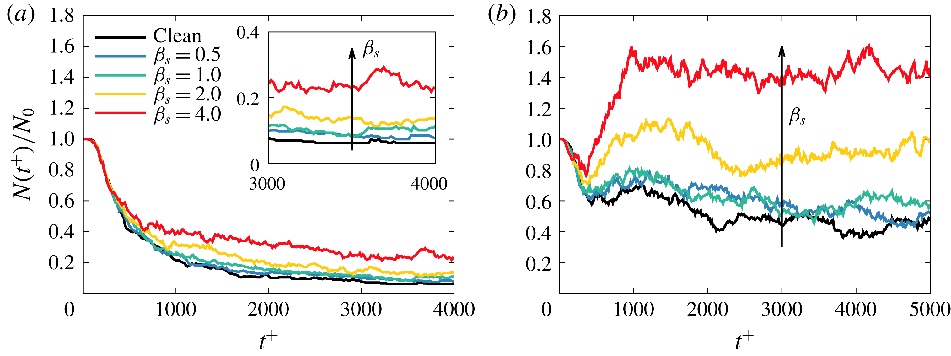
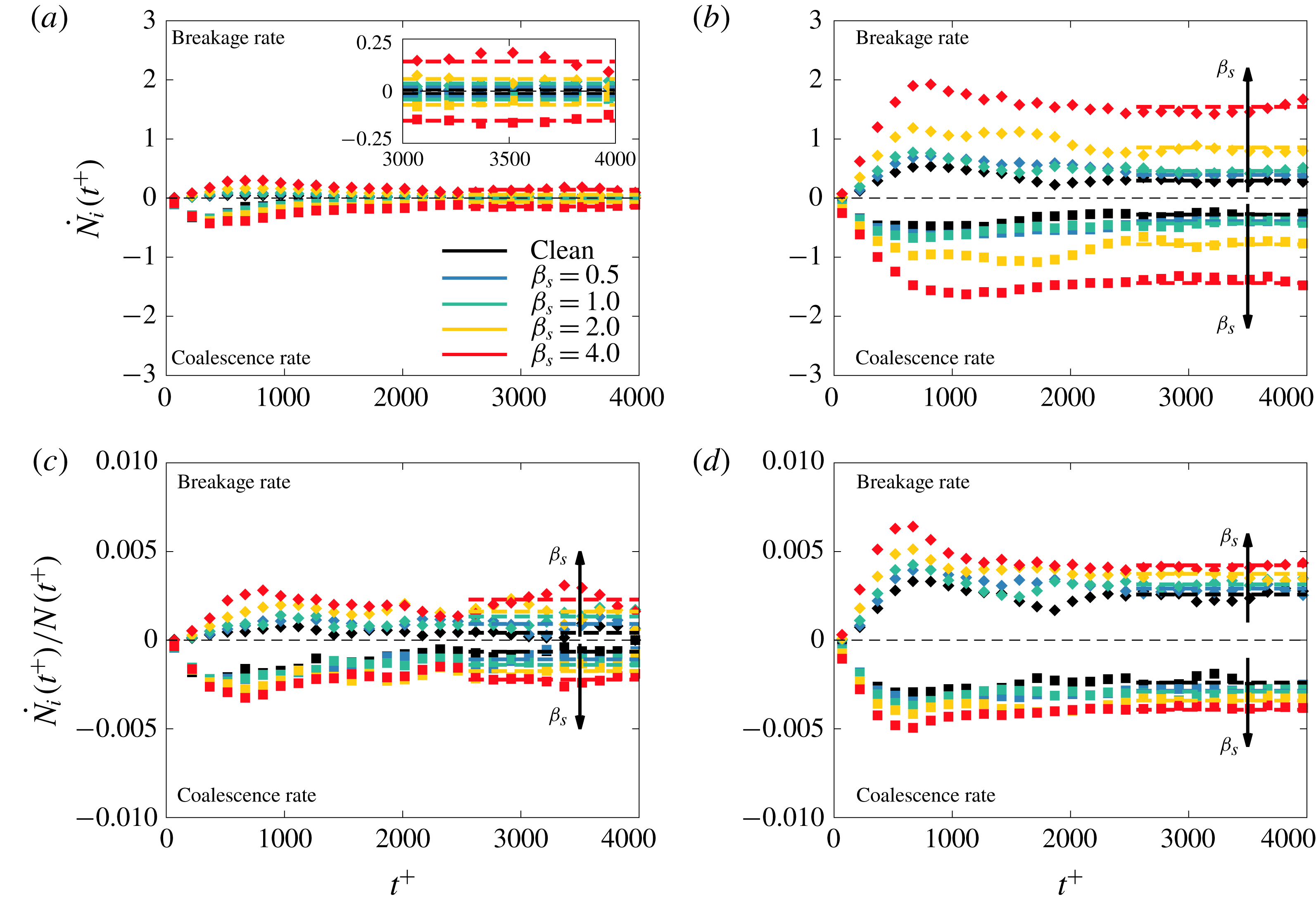
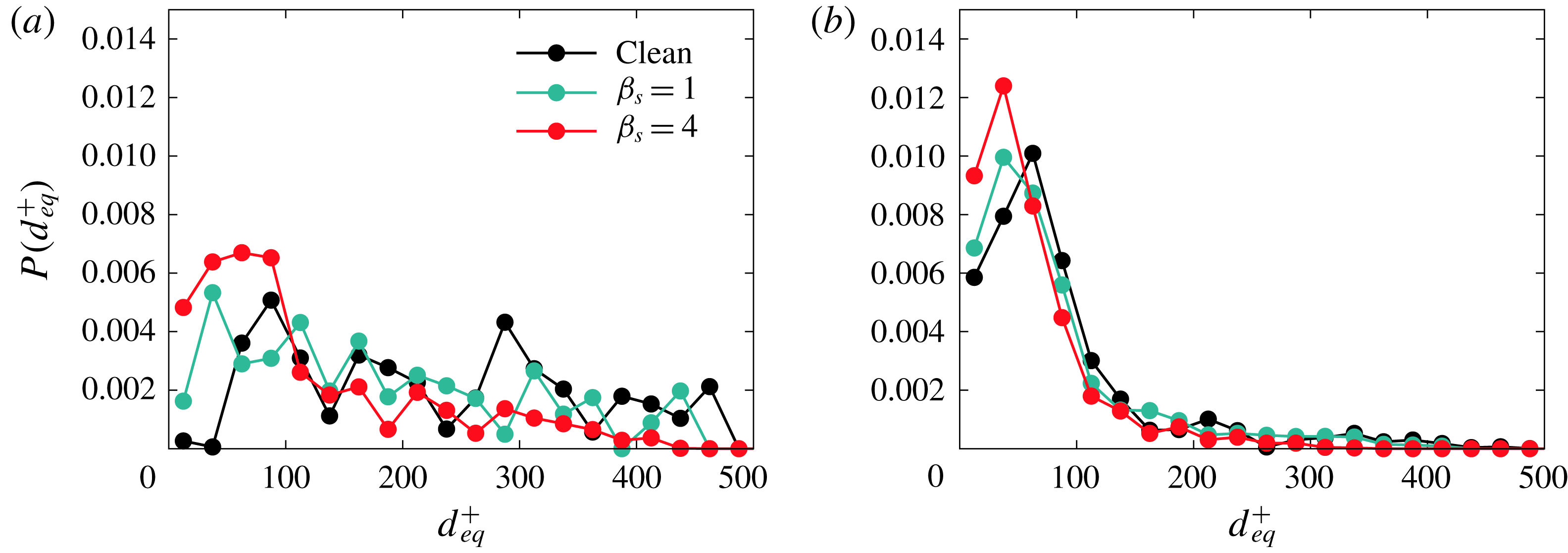
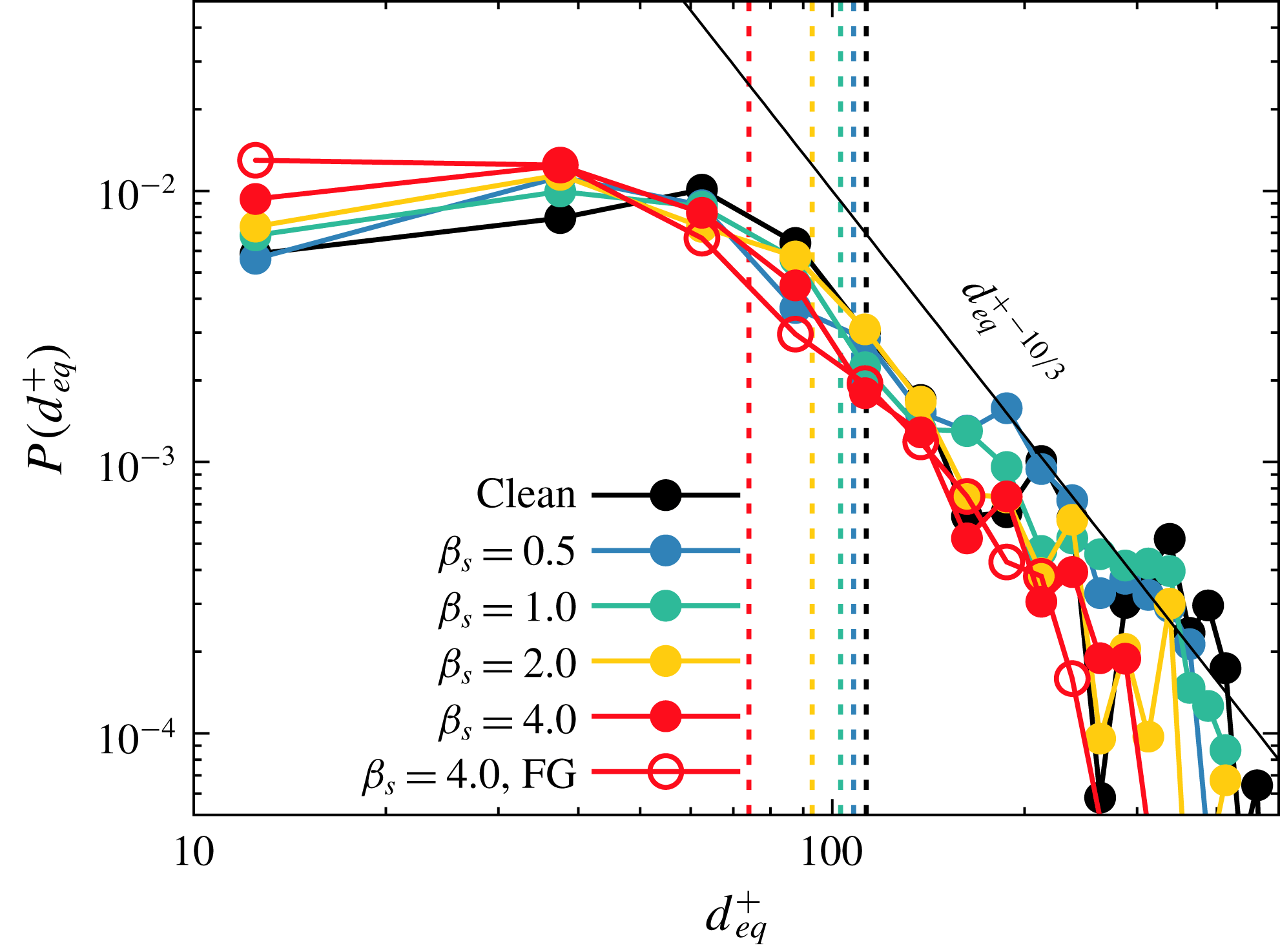
1 Introduction
The accurate prediction of momentum, heat and mass transfer through an interface is a fundamental problem in a wide range of industrial applications and in nature (Kralova & Sjöblom Reference Kralova and Sjöblom2009; Rosen & Kunjappu Reference Rosen and Kunjappu2012; Pereira et al. Reference Pereira, Ashton, Sabbaghzadeh, Shutler and Upstill-Goddard2018). Mathematical models and empirical correlations based on macroscopic observables, such as shape and extension of the interface, are often used to estimate these transfer rates (Kiyomi & Fumitake Reference Kiyomi and Fumitake1974; Kelly & Kazimi Reference Kelly and Kazimi1982; Delhaye & Bricard Reference Delhaye and Bricard1994); these correlations, though mostly tuned on experimental data, can often provide a first estimate of transfer rates. To improve the accuracy of these predictions and to gain a better comprehension of the underlying physics, the development of numerical tools capable of performing high-fidelity simulations is highly desirable, and perhaps possible to achieve these days.
In this paper, we focus on the simulation of breakage, coalescence and ultimately the size distribution of surfactant-laden droplets in turbulent flow. This problem is characterized by a physics acting at many different scales: from the molecular scale of the interface, to the Kolmogorov scale and up to the largest problem scales. Today’s computational methods can handle a scale separation of about three or four orders of magnitude between large and small turbulence scales, but the scale separation between interfacial phenomena and the smallest turbulence scales is about another five orders of magnitude. Naturally, in these types of problems, it is impossible to set the numerical resolution to the interfacial scale: there is not enough computational power available. Therefore, in the recent past, several numerical techniques have been developed to overcome the multiscale aspects of this problem. Broadly speaking, these methods can be categorized as interface-tracking methods and interface-capturing methods. Interface-tracking methods rely on the advection of a set of Lagrangian marker points, which define the instantaneous position of the interface. These methods proved to be excellent in the simulation of droplets and bubbles in turbulence (Lu & Tryggvason Reference Lu and Tryggvason2008) and, recently, their capability has been extended to model surfactant-laden droplets (Lu, Muradoglu & Tryggvason Reference Lu, Muradoglu and Tryggvason2017) and coalescing interfaces (Lu & Tryggvason Reference Lu and Tryggvason2018). The downside of these methods, however, is that closure models are needed to capture interface interactions (e.g. coalescence) and complex re-meshing algorithms are required to describe the interfacial dynamics. The other category, interface-capturing methods, includes several types of approach, such as the volume of fluid method (Hirt & Nichols Reference Hirt and Nichols1981), the level-set method (Fedkiw et al. Reference Fedkiw, Aslam, Merriman and Osher1999), the lattice Boltzmann method (Shan & Chen Reference Shan and Chen1993; He, Chen & Zhang Reference He, Chen and Zhang1999) and the phase-field method (Anderson, McFadden & Wheeler Reference Anderson, McFadden and Wheeler1998; Jacqmin Reference Jacqmin1999). We refer the reader to Scardovelli & Zaleski (Reference Scardovelli and Zaleski1999) for a review of the volume of fluid method, to Gibou, Fedkiw & Osher (Reference Gibou, Fedkiw and Osher2018) for the level-set method and to Chen & Doolen (Reference Chen and Doolen1998) for lattice-Boltzmann-based methods. Interested readers can find in Scarbolo et al. (Reference Scarbolo, Molin, Perlekar, Sbragaglia, Soldati and Toschi2013) a benchmark comparison between lattice Boltzmann and phase-field methods.
In this work, we exploit the phase-field method (Anderson et al. Reference Anderson, McFadden and Wheeler1998; Jacqmin Reference Jacqmin1999), which is characterized by a strong physical foundation: the method is indeed the natural extension of the van der Waals theory of critical phenomena (van der Waals Reference van der Waals1979), and its thermodynamic derivation, which is rigorous for near-critical mixtures, allowing the description of interface creation, breakage and merging in a physically grounded framework. In the framework of the phase-field method, a scalar order parameter (phase field) describes the local concentration of the two phases; the order parameter has a constant value in the bulk of each phase, and undergoes a smooth transition across a thin interfacial layer. The spatial and temporal evolution of the order parameter is governed by a Cahn–Hilliard equation (Cahn & Hilliard Reference Cahn and Hilliard1958, Reference Cahn and Hilliard1959a ,Reference Cahn and Hilliard b ), which builds on a chemical potential derived from a free energy functional.
Most previous investigations of the interactions between large droplets and turbulence have been based on pure fluids (Elghobashi Reference Elghobashi2019) with only a few works (Skartlien, Sollum & Schumann Reference Skartlien, Sollum and Schumann2013; Lu et al. Reference Lu, Muradoglu and Tryggvason2017) considering also the presence of surface-active agents (surfactants). However, real applications are always characterized by the presence of impurities or surfactants, which locally modify the surface tension value. Surfactant molecules are amphiphilic, so they have polar heads and non-polar tails. Amphiphilic molecules tend to accumulate at interfaces, where they produce a local decrease of the surface tension. The description of surfactants and of their effects on the multiphase flow adds further complexity to the problem: an additional variable, the surfactant concentration, has to be computed over a deformable, topologically changing and ever-moving interface. Only a few numerical methods capable of describing the dynamics of surfactant-laden interfaces have been proposed. In particular, extensions to the methods previously presented for surfactant-free multiphase flows have been developed in recent years for the front-tracking method (Muradoglu & Tryggvason Reference Muradoglu and Tryggvason2014; Lu et al. Reference Lu, Muradoglu and Tryggvason2017), immersed boundary method (Lai, Tseng & Huang Reference Lai, Tseng and Huang2008, Reference Lai, Tseng and Huang2010), volume of fluid method (Renardy, Renardy & Cristini Reference Renardy, Renardy and Cristini2002; James & Lowengrub Reference James and Lowengrub2004), level-set method (Xu & Zhao Reference Xu and Zhao2003; Xu et al. Reference Xu, Zhilin, Lowengrub and Zhao2006; Piedfert et al. Reference Piedfert, Lalanne, Masbernat and Risso2018), lattice Boltzmann method (Farhat et al. Reference Farhat, Celiker, Singh and Lee2011; Liu et al. Reference Liu, Ba, Wu, Li, Xi and Zhang2018) and phase-field method (Komura & Kodama Reference Komura and Kodama1997; Engblom et al. Reference Engblom, Do-Quang, Amberg and Tornberg2013). In the framework of the phase-field method, the presence of a soluble surfactant can be considered by introducing an additional order parameter, which describes the surfactant concentration in the entire domain. In particular, this scalar variable is uniform in the bulk of the two phases and reaches its maximum value at the interface (where surfactant molecules accumulate preferentially). With respect to other available approaches, the phase-field framework allows for the description of surfactant dynamics (including also adsorption/desorption phenomena) by adding an extra order parameter and, in general, allows one to avoid complex re-meshing algorithms when dealing with topological changes.
In this work, we employ a two-order-parameter formulation of the phase-field method (Engblom et al.
Reference Engblom, Do-Quang, Amberg and Tornberg2013; Yun, Li & Kim Reference Yun, Li and Kim2014; Soligo, Roccon & Soldati Reference Soligo, Roccon and Soldati2019a
) to describe the dynamics of a surfactant-laden system. A first order parameter, the phase field
 $\unicode[STIX]{x1D719}$
, describes the dispersed phase morphology, while a second order parameter
 $\unicode[STIX]{x1D713}$
describes the surfactant concentration in the entire system. The phase-field method is coupled with direct numerical simulation of turbulence to study the behaviour of a swarm of surfactant-laden droplets in a turbulent channel flow at a constant shear Reynolds number. Specifically, we consider droplets characterized by two different values of surface tension (clean interface), set with the Weber number (ratio between inertial and surface tension forces), and four different surfactant strengths, set with the elasticity number (parameter that quantifies the magnitude of surface tension reduction produced by the surfactant). To obtain a complete benchmark, we also consider two clean (surfactant-free) systems in which surface tension is constant. Our results indicate that the addition of a soluble surfactant strongly modifies the morphology of the dispersed phase, especially when stronger surfactants (larger elasticity numbers) are considered. Using quantitative statistics and qualitative physical insights, we are able to describe the distribution of the surfactant over the interface of the droplets and to characterize the modifications produced by the surfactant in the number of droplets, coalescence and breakage rates, and droplet size distribution (DSD).
The paper is organized as follows. First, the governing equations and the numerical method are presented in § 2. The outcome of the simulations is presented in § 3; in the first part the effects of the Weber and elasticity numbers on the surfactant concentration are detailed, while in the second part we focus on their effect on the morphology of the dispersed phase, analysing the droplet population balance and the DSD. Lastly, conclusions are drawn in § 4.
2 Methodology
The dynamics of the multiphase turbulent flow is described with direct numerical simulation of the Navier–Stokes equations coupled with a modified phase-field method used in a two-order-parameter formulation (Komura & Kodama Reference Komura and Kodama1997; Engblom et al. Reference Engblom, Do-Quang, Amberg and Tornberg2013; Yun et al. Reference Yun, Li and Kim2014; Soligo et al. Reference Soligo, Roccon and Soldati2019a ). The Navier–Stokes equations, suitably modified to account for the presence of a surfactant-laden interface, describe the flow field while the phase-field method is used to compute the morphology of the dispersed phase and the surfactant concentration.
2.1 Computational modelling of interface morphology and surfactant concentration
In the framework of the phase-field method, two scalar order parameters are used to describe the dispersed-phase morphology and the surfactant concentration. A first order parameter, the phase field,
 $\unicode[STIX]{x1D719}$
, describes the interface shape and position. The phase field has a uniform value in the bulk of each phase and undergoes a smooth transition across the thin interfacial layer. A second order parameter,
 $\unicode[STIX]{x1D713}$
, is used to describe the surfactant concentration (Laradji et al.
Reference Laradji, Guo, Grant and Zuckermann1992; Komura & Kodama Reference Komura and Kodama1997). The surfactant concentration has a low uniform value in the bulk of the two phases, while at the interface it reaches its maximum value. Indeed, surfactant molecules, because of their amphiphilic nature (hydrophobic tails and hydrophilic heads), preferentially accumulate at the interface. The phase field and the surfactant concentration dynamics are described by two Cahn–Hilliard-like equations, which in dimensionless form (see appendix A for details) read as
 $$\begin{eqnarray}\displaystyle & \displaystyle \frac{\unicode[STIX]{x2202}\unicode[STIX]{x1D719}}{\unicode[STIX]{x2202}t}+\boldsymbol{u}\boldsymbol{\cdot }\unicode[STIX]{x1D735}\unicode[STIX]{x1D719}=\frac{1}{Pe_{\unicode[STIX]{x1D719}}}\unicode[STIX]{x1D6FB}^{2}\unicode[STIX]{x1D707}_{\unicode[STIX]{x1D719}}+f_{p}, & \displaystyle\end{eqnarray}$$
 $$\begin{eqnarray}\displaystyle & \displaystyle \frac{\unicode[STIX]{x2202}\unicode[STIX]{x1D713}}{\unicode[STIX]{x2202}t}+\boldsymbol{u}\boldsymbol{\cdot }\unicode[STIX]{x1D735}\unicode[STIX]{x1D713}=\frac{1}{Pe_{\unicode[STIX]{x1D713}}}\unicode[STIX]{x1D735}\boldsymbol{\cdot }[\unicode[STIX]{x1D713}(1-\unicode[STIX]{x1D713})\unicode[STIX]{x1D735}\unicode[STIX]{x1D707}_{\unicode[STIX]{x1D713}}], & \displaystyle\end{eqnarray}$$
where
 $\boldsymbol{u}=(u,v,w)$
is the velocity field,
 $Pe_{\unicode[STIX]{x1D719}}$
and
 $Pe_{\unicode[STIX]{x1D713}}$
are the phase-field and the surfactant Péclet numbers and
 $\unicode[STIX]{x1D707}_{\unicode[STIX]{x1D719}}$
and
 $\unicode[STIX]{x1D707}_{\unicode[STIX]{x1D713}}$
are the respective chemical potentials. The two Péclet numbers are defined as follows:
 $$\begin{eqnarray}Pe_{\unicode[STIX]{x1D719}}=\frac{u_{\unicode[STIX]{x1D70F}}h}{{\mathcal{M}}_{\unicode[STIX]{x1D719}}\unicode[STIX]{x1D6FD}},\quad Pe_{\unicode[STIX]{x1D713}}=\frac{u_{\unicode[STIX]{x1D70F}}h\unicode[STIX]{x1D6FC}}{{\mathcal{M}}_{\unicode[STIX]{x1D713}}\unicode[STIX]{x1D6FD}^{2}},\end{eqnarray}$$
where
 $u_{\unicode[STIX]{x1D70F}}$
is the friction velocity,
 $h$
the channel half-height,
 ${\mathcal{M}}_{\unicode[STIX]{x1D719}}$
and
 ${\mathcal{M}}_{\unicode[STIX]{x1D713}}$
, respectively, the phase-field and the surfactant mobilities and
 $\unicode[STIX]{x1D6FC}$
and
 $\unicode[STIX]{x1D6FD}$
positive constants (see appendix A). These two dimensionless parameters represent the ratio between the diffusive time scale,
 $h^{2}/({\mathcal{M}}_{\unicode[STIX]{x1D719},\unicode[STIX]{x1D713}}\unicode[STIX]{x1D6FD}^{2})$
, and the convective time scale,
 $h/u_{\unicode[STIX]{x1D70F}}$
. The term
 $f_{p}$
is the penalty flux of the profile-corrected formulation of the phase-field method (Li, Choi & Kim Reference Li, Choi and Kim2016; Zhang & Ye Reference Zhang and Ye2017; Soligo, Roccon & Soldati Reference Soligo, Roccon and Soldati2019b
). The adoption of this formulation allows for a better conservation of the interfacial profile and to overcome some drawbacks (e.g. mass leakage among the phases, coarsening and misrepresentation of the interfacial profile) present in the standard formulation of the phase-field method (Yue, Zhou & Feng Reference Yue, Zhou and Feng2007; Li et al.
Reference Li, Choi and Kim2016). The penalty flux is defined as follows (Li et al.
Reference Li, Choi and Kim2016):
 $$\begin{eqnarray}f_{p}=\frac{\unicode[STIX]{x1D706}}{Pe_{\unicode[STIX]{x1D719}}}\left[\unicode[STIX]{x1D6FB}^{2}\unicode[STIX]{x1D719}-\frac{1}{\sqrt{2}Ch}\unicode[STIX]{x1D735}\boldsymbol{\cdot }\left((1-\unicode[STIX]{x1D719}^{2})\frac{\unicode[STIX]{x1D735}\unicode[STIX]{x1D719}}{|\unicode[STIX]{x1D735}\unicode[STIX]{x1D719}|}\right)\right],\end{eqnarray}$$
where the numerical parameter
 $\unicode[STIX]{x1D706}$
is set via a suitable scaling (Soligo et al.
Reference Soligo, Roccon and Soldati2019b
).
The expression of the chemical potentials
 $\unicode[STIX]{x1D707}_{\unicode[STIX]{x1D719}}$
and
 $\unicode[STIX]{x1D707}_{\unicode[STIX]{x1D713}}$
is derived considering a two-order-parameter Ginzburg–Landau free energy functional,
 ${\mathcal{F}}[\unicode[STIX]{x1D719},\unicode[STIX]{x1D735}\unicode[STIX]{x1D719},\unicode[STIX]{x1D713}]$
. The functional is composed of the sum of five different contributions:
 $$\begin{eqnarray}{\mathcal{F}}[\unicode[STIX]{x1D719},\unicode[STIX]{x1D735}\unicode[STIX]{x1D719},\unicode[STIX]{x1D713}]=\int _{\unicode[STIX]{x1D6FA}}(f_{0}+f_{m}+f_{\unicode[STIX]{x1D713}}+f_{1}+f_{b})\,\text{d}\unicode[STIX]{x1D6FA},\end{eqnarray}$$
where
 $\unicode[STIX]{x1D6FA}$
is the domain considered. The various contributions to the free energy functional are defined as
 $$\begin{eqnarray}\displaystyle & \displaystyle f_{0}={\textstyle \frac{1}{4}}(\unicode[STIX]{x1D719}-1)^{2}(\unicode[STIX]{x1D719}+1)^{2}, & \displaystyle\end{eqnarray}$$
 $$\begin{eqnarray}\displaystyle & \displaystyle f_{m}=\frac{Ch^{2}}{2}|\unicode[STIX]{x1D735}\unicode[STIX]{x1D719}|^{2}\,, & \displaystyle\end{eqnarray}$$
 $$\begin{eqnarray}\displaystyle & \displaystyle f_{\unicode[STIX]{x1D713}}=Pi[\unicode[STIX]{x1D713}\log \unicode[STIX]{x1D713}+(1-\unicode[STIX]{x1D713})\log (1-\unicode[STIX]{x1D713})], & \displaystyle\end{eqnarray}$$
 $$\begin{eqnarray}\displaystyle & \displaystyle f_{1}=-{\textstyle \frac{1}{2}}\unicode[STIX]{x1D713}(1-\unicode[STIX]{x1D719}^{2})^{2}, & \displaystyle\end{eqnarray}$$
 $$\begin{eqnarray}\displaystyle & \displaystyle f_{b}=\frac{1}{2E_{x}}\unicode[STIX]{x1D719}^{2}\unicode[STIX]{x1D713}. & \displaystyle\end{eqnarray}$$
The first two terms,
 $f_{0}$
and
 $f_{m}$
, are functions of the phase field only; their expression matches exactly that used in the analysis of clean systems (Scarbolo, Bianco & Soldati Reference Scarbolo, Bianco and Soldati2015; Roccon et al.
Reference Roccon, De Paoli, Zonta and Soldati2017; Roccon, Zonta & Soldati Reference Roccon, Zonta and Soldati2019). The term
 $f_{0}$
describes the phobic behaviour of the two fluids: a double-well potential (whose minima correspond to the two pure phases) accounts for the tendency of the system to separate into pure phases. The interfacial term,
 $f_{m}$
, accounts for the energy stored in the interfacial layer (i.e. the surface tension). The Cahn number,
 $Ch=\unicode[STIX]{x1D709}/h$
, is the ratio between the interface length scale,
 $\unicode[STIX]{x1D709}=\sqrt{\unicode[STIX]{x1D705}/\unicode[STIX]{x1D6FD}}$
, and the problem length scale,
 $h$
, while
 $\unicode[STIX]{x1D705}$
is a positive constant (see appendix A). The Cahn number sets the thickness of the thin interfacial layer. The three latter terms describe the surfactant dynamics. The entropy term,
 $f_{\unicode[STIX]{x1D713}}$
, describes the entropy decrease obtained when the surfactant uniformly distributes in the entire domain. The temperature-dependent parameter,
 $Pi=\unicode[STIX]{x1D705}T\unicode[STIX]{x1D6FC}/\unicode[STIX]{x1D6FD}^{2}$
, defines the surfactant diffusivity; larger values of
 $Pi$
(higher temperatures) promote a more uniform surfactant distribution in all the domain. This term strictly bounds the surfactant concentration between
 $\unicode[STIX]{x1D713}=0$
(absence of surfactant) and
 $\unicode[STIX]{x1D713}=1$
(saturation of surfactant). The surfactant adsorption term,
 $f_{1}$
, accounts for the amphiphilic behaviour and favours the collection of surfactant molecules at the interface. The contribution of the adsorption term is important at the interface, while it vanishes in the bulk of the two phases. The last contribution,
 $f_{b}$
, controls the solubility of the surfactant in the bulk of the two phases. This term has negligible contribution at the interface, while it is more effective in the bulk of the phases. The surfactant solubility parameter,
 $E_{x}=\unicode[STIX]{x1D6FD}/w_{b}$
, defines the solubility of the surfactant: larger values of
 $E_{x}$
correspond to a greater solubility of the surfactant in the bulk regions. For a complete description of all the various quantities, see appendix A.
The expressions of the two chemical potentials,
 $\unicode[STIX]{x1D707}_{\unicode[STIX]{x1D719}}$
and
 $\unicode[STIX]{x1D707}_{\unicode[STIX]{x1D713}}$
, are obtained by taking the variational derivative of the free energy functional with respect to each order parameter:
 $$\begin{eqnarray}\displaystyle & \displaystyle \unicode[STIX]{x1D707}_{\unicode[STIX]{x1D719}}=\frac{\unicode[STIX]{x1D6FF}{\mathcal{F}}[\unicode[STIX]{x1D719},\unicode[STIX]{x1D735}\unicode[STIX]{x1D719},\unicode[STIX]{x1D713}]}{\unicode[STIX]{x1D6FF}\unicode[STIX]{x1D719}}=\unicode[STIX]{x1D719}^{3}-\unicode[STIX]{x1D719}-Ch^{2}\unicode[STIX]{x1D6FB}^{2}\unicode[STIX]{x1D719}+\underbrace{Ch^{2}(\unicode[STIX]{x1D713}\unicode[STIX]{x1D6FB}^{2}\unicode[STIX]{x1D719}+\unicode[STIX]{x1D735}\unicode[STIX]{x1D713}\boldsymbol{\cdot }\unicode[STIX]{x1D735}\unicode[STIX]{x1D719})+\frac{1}{E_{x}}\unicode[STIX]{x1D719}\unicode[STIX]{x1D713}}_{C_{\unicode[STIX]{x1D719}\unicode[STIX]{x1D713}}},\qquad & \displaystyle\end{eqnarray}$$
 $$\begin{eqnarray}\displaystyle & \displaystyle \unicode[STIX]{x1D707}_{\unicode[STIX]{x1D713}}=\frac{\unicode[STIX]{x1D6FF}{\mathcal{F}}[\unicode[STIX]{x1D719},\unicode[STIX]{x1D735}\unicode[STIX]{x1D719},\unicode[STIX]{x1D713}]}{\unicode[STIX]{x1D6FF}\unicode[STIX]{x1D713}}=Pi\log \left(\frac{\unicode[STIX]{x1D713}}{1-\unicode[STIX]{x1D713}}\right)-\frac{(1-\unicode[STIX]{x1D719}^{2})^{2}}{2}+\frac{\unicode[STIX]{x1D719}^{2}}{2E_{x}}. & \displaystyle\end{eqnarray}$$
The term
 $C_{\unicode[STIX]{x1D719}\unicode[STIX]{x1D713}}$
may lead to an unphysical behaviour of the thin interfacial layer: to restore the correct interfacial behaviour,
 $C_{\unicode[STIX]{x1D719}\unicode[STIX]{x1D713}}$
has been neglected according to Yun et al. (Reference Yun, Li and Kim2014), and, therefore, surface tension forces are computed using a geometrical approach (Popinet Reference Popinet2018), which relies on the phase field to compute the interface curvature, together with an equation of state (EOS) describing the surfactant effect on surface tension (Yun et al.
Reference Yun, Li and Kim2014). This approach, compared to the thermodynamical one (Laradji et al.
Reference Laradji, Guo, Grant and Zuckermann1992; Engblom et al.
Reference Engblom, Do-Quang, Amberg and Tornberg2013), improves the flexibility of the method since surfactant action on surface tension is completely customizable via the surface tension EOS. From the expression of the chemical potentials, the equilibrium profiles for the two order parameters can be derived; at equilibrium,
 $\unicode[STIX]{x1D707}_{\unicode[STIX]{x1D719}}$
and
 $\unicode[STIX]{x1D707}_{\unicode[STIX]{x1D713}}$
are uniform in the entire domain, and therefore
 $$\begin{eqnarray}\unicode[STIX]{x1D735}\unicode[STIX]{x1D707}_{\unicode[STIX]{x1D719}}=\mathbf{0},\quad \unicode[STIX]{x1D735}\unicode[STIX]{x1D707}_{\unicode[STIX]{x1D713}}=\mathbf{0}.\end{eqnarray}$$
Considering a planar interface located at
 $x=0$
(where
 $x$
is the direction normal to the interface), an analytic solution can be derived for both of the order parameters
 $$\begin{eqnarray}\unicode[STIX]{x1D719}(s)=\tanh \left(\frac{s}{\sqrt{2}Ch}\right),\end{eqnarray}$$
 $$\begin{eqnarray}\unicode[STIX]{x1D713}(\unicode[STIX]{x1D719})=\frac{\unicode[STIX]{x1D713}_{b}}{\unicode[STIX]{x1D713}_{b}+\unicode[STIX]{x1D713}_{c}(\unicode[STIX]{x1D719})(1-\unicode[STIX]{x1D713}_{b})},\end{eqnarray}$$
where
 $s$
is the coordinate normal to the interface. The auxiliary variable,
 $\unicode[STIX]{x1D713}_{c}$
, is a function of the phase field, and it is defined as follows:
 $$\begin{eqnarray}\unicode[STIX]{x1D713}_{c}(\unicode[STIX]{x1D719})=\exp \left[-\frac{1-\unicode[STIX]{x1D719}^{2}}{2Pi}\left(1-\unicode[STIX]{x1D719}^{2}+\frac{1}{E_{x}}\right)\right].\end{eqnarray}$$
The phase field is uniform in the bulk of the two phases (
 $\unicode[STIX]{x1D719}\pm 1$
) and it undergoes a smooth transition following a hyperbolic tangent profile across the interface. Similarly, the surfactant concentration is uniform in the bulk of the two phases (surfactant bulk concentration,
 $\unicode[STIX]{x1D713}_{b}$
) and reaches its maximum value at the interface (peak value,
 $\unicode[STIX]{x1D713}_{0}$
). The peak value
 $\unicode[STIX]{x1D713}_{0}$
is influenced by the surfactant parameters
 $Pi$
and
 $E_{x}$
, and by the surfactant bulk concentration,
 $\unicode[STIX]{x1D713}_{b}$
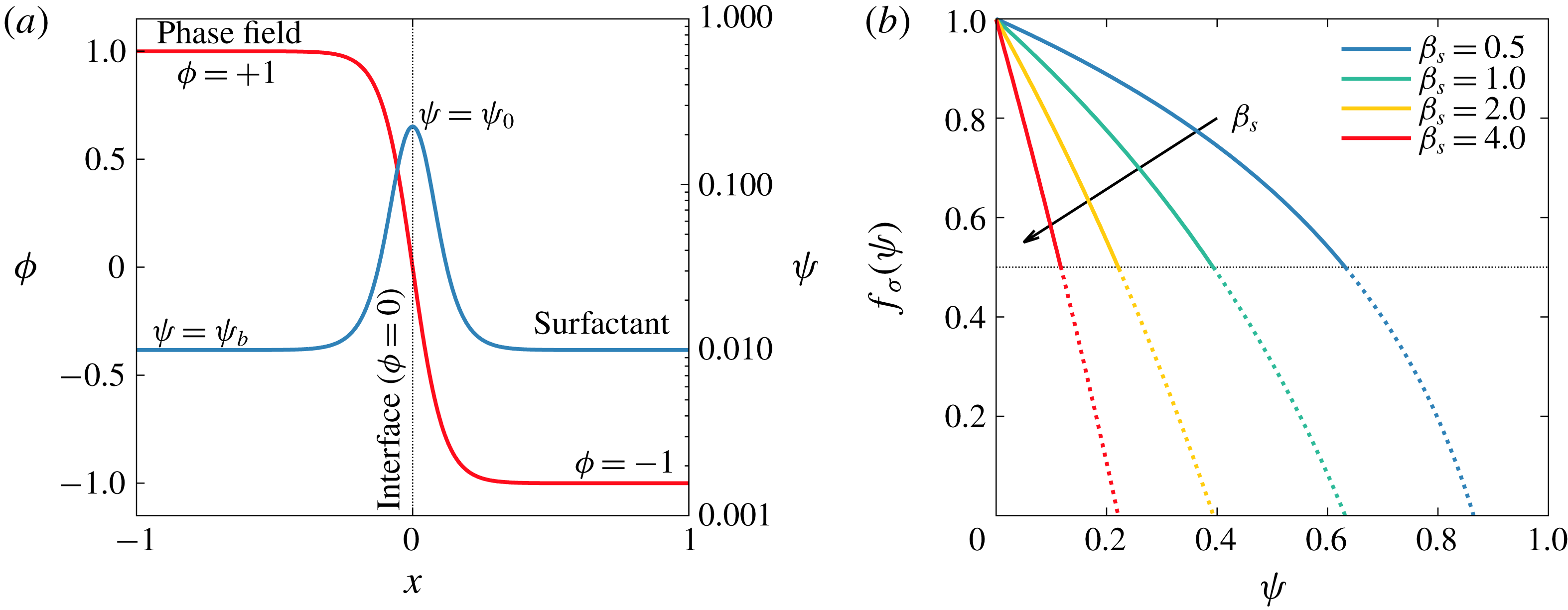
, as indicated by (2.11)–(2.12). The two equilibrium profiles are shown in figure 1(a): the phase field is shown in red (linear scale on the left-hand axis), while the surfactant concentration is shown in blue (logarithmic scale on the right-hand axis).
(a) Equilibrium profiles for the phase field (red, linear scale on the left-hand axis) and for the surfactant concentration (blue, logarithmic scale on the right-hand axis). The phase field is uniform in the bulk (
 $\unicode[STIX]{x1D719}=\pm 1$
) and undergoes a smooth transition following a hyperbolic tangent profile across the interface. The surfactant concentration is uniform in the bulk (
 $\unicode[STIX]{x1D713}=\unicode[STIX]{x1D713}_{b}$
) and reaches its peak at the interface (
 $\unicode[STIX]{x1D713}=\unicode[STIX]{x1D713}_{0}$
). (b) Modified Langmuir EOS for different elasticity numbers
 $\unicode[STIX]{x1D6FD}_{s}$
. A stronger surfactant (larger
 $\unicode[STIX]{x1D6FD}_{s}$
) introduces a considerable surface tension reduction even for low concentrations. The surface tension decrease is bounded to
 $f_{\unicode[STIX]{x1D70E}}=0.5$
(thin dashed black line). Indeed, according to experiments, surface tension does not decrease below this threshold (roughly).

2.2 Hydrodynamics
To describe the hydrodynamics of the multiphase system, the phase field and the surfactant concentration transport equations have been coupled with the Navier–Stokes equations. The presence of a surfactant-laden interface and of the accompanying forces are accounted for by introducing an interfacial term in the Navier–Stokes equations. Here, surface tension forces are calculated adopting a geometrical approach (Yun et al.
Reference Yun, Li and Kim2014): the curvature of the interface is calculated using the Korteweg tensor (Korteweg Reference Korteweg1901) while an EOS is used to describe the surface tension reduction produced by the surfactant. In this work, to focus on the effects of the surfactant, we consider two phases with matched density (
 $\unicode[STIX]{x1D70C}=\unicode[STIX]{x1D70C}_{1}=\unicode[STIX]{x1D70C}_{2}$
) and viscosity (
 $\unicode[STIX]{x1D707}=\unicode[STIX]{x1D707}_{1}=\unicode[STIX]{x1D707}_{2}$
). With these assumptions, the continuity and Navier–Stokes equations result in
 $$\begin{eqnarray}\unicode[STIX]{x1D735}\boldsymbol{\cdot }\boldsymbol{u}=0,\end{eqnarray}$$
 $$\begin{eqnarray}\frac{\unicode[STIX]{x2202}\boldsymbol{u}}{\unicode[STIX]{x2202}t}+\boldsymbol{u}\boldsymbol{\cdot }\unicode[STIX]{x1D735}\boldsymbol{u}=-\unicode[STIX]{x1D735}p+\frac{1}{Re_{\unicode[STIX]{x1D70F}}}\unicode[STIX]{x1D6FB}^{2}\boldsymbol{u}+\frac{3}{\sqrt{8}}\frac{Ch}{We}\unicode[STIX]{x1D735}\boldsymbol{\cdot }[f_{\unicode[STIX]{x1D70E}}(\unicode[STIX]{x1D713})\unicode[STIX]{x1D64F}_{c}],\end{eqnarray}$$
where
 $\boldsymbol{u}=(u,v,w)$
is the velocity field,
 $\unicode[STIX]{x1D735}p$
is the pressure gradient (including also the mean pressure gradient that drives the flow; see Soldati & Banerjee (Reference Soldati and Banerjee1998)),
 $\unicode[STIX]{x1D64F}_{c}=|\unicode[STIX]{x1D735}\unicode[STIX]{x1D719}|^{2}\boldsymbol{I}-\unicode[STIX]{x1D735}\unicode[STIX]{x1D719}\otimes \unicode[STIX]{x1D735}\unicode[STIX]{x1D719}$
is the Korteweg tensor and
 $f_{\unicode[STIX]{x1D70E}}(\unicode[STIX]{x1D713})$
is the surface tension EOS (Chang & Franses Reference Chang and Franses1995; Bazhlekov, Anderson & Meijer Reference Bazhlekov, Anderson and Meijer2006). The last term, which includes the Korteweg tensor and the surface tension EOS, accounts for the interfacial forces induced by the surfactant-laden interface on the flow. This term can be split in a component normal to the interface (capillary) and one tangential to the interface (Marangoni):
 $$\begin{eqnarray}\unicode[STIX]{x1D735}\boldsymbol{\cdot }[f_{\unicode[STIX]{x1D70E}}(\unicode[STIX]{x1D713})\unicode[STIX]{x1D64F}_{c}]=\underbrace{f_{\unicode[STIX]{x1D70E}}(\unicode[STIX]{x1D713})\unicode[STIX]{x1D735}\boldsymbol{\cdot }\unicode[STIX]{x1D64F}_{c}}_{Normal~(capillary)}+\underbrace{\unicode[STIX]{x1D735}f_{\unicode[STIX]{x1D70E}}(\unicode[STIX]{x1D713})\boldsymbol{\cdot }\unicode[STIX]{x1D64F}_{c}\,}_{Tangential~(Marangoni)}\!.\end{eqnarray}$$
When surface tension is constant, the Marangoni contribution vanishes, leaving only the capillary (normal) contribution.
The dimensionless groups appearing in (2.14) are the shear Reynolds number and the Weber number. The Reynolds number,
 $Re_{\unicode[STIX]{x1D70F}}=\unicode[STIX]{x1D70C}u_{\unicode[STIX]{x1D70F}}h/\unicode[STIX]{x1D707}$
, is the ratio between inertial and viscous forces, where
 $u_{\unicode[STIX]{x1D70F}}=\sqrt{\unicode[STIX]{x1D70F}_{w}/\unicode[STIX]{x1D70C}}$
is the friction velocity,
 $\unicode[STIX]{x1D70F}_{w}$
the mean wall-shear stress,
 $\unicode[STIX]{x1D70C}$
the density,
 $\unicode[STIX]{x1D707}$
the viscosity and
 $h$
the channel half-height. The Weber number,
 $We=\unicode[STIX]{x1D70C}u_{\unicode[STIX]{x1D70F}}^{2}h/\unicode[STIX]{x1D70E}_{0}$
, is the ratio between inertial and surface tension forces and it is computed using as a reference the surface tension of a clean interface,
 $\unicode[STIX]{x1D70E}_{0}$
.
The EOS adopted in this work is a modified version of the Langmuir EOS. While at low surfactant concentrations the original Langmuir EOS well follows the experimental measurements, there are experimental evidences for liquid–liquid (López-Díaz, García-Mateos & Velázquez Reference López-Díaz, García-Mateos and Velázquez2006; Ju et al. Reference Ju, Jiang, Geng, Wang and Zhang2017) and gas–liquid (Chang & Franses Reference Chang and Franses1995) systems showing that surface tension never decreases below about 30 % to 60 % of the clean interface surface tension for any surfactant concentration. This is a consequence of the saturation of the interface: once a monolayer of surfactant molecules is formed over the interface, no more surfactant can collect there and, thus, surface tension remains constant (Porter Reference Porter1991, p. 26). The Langmuir EOS, however, predicts an unbounded surface tension decrease for increasing surfactant concentrations. Thus, we use a modified EOS, in which the minimum surface tension value was set to half the clean interface surface tension; while this value was arbitrarily chosen, it was selected within the range of measured values (Chang & Franses Reference Chang and Franses1995; López-Díaz et al. Reference López-Díaz, García-Mateos and Velázquez2006; Ju et al. Reference Ju, Jiang, Geng, Wang and Zhang2017). The modified Langmuir EOS adopted in this work is
 $$\begin{eqnarray}f_{\unicode[STIX]{x1D70E}}(\unicode[STIX]{x1D713})=\frac{\unicode[STIX]{x1D70E}(\unicode[STIX]{x1D713})}{\unicode[STIX]{x1D70E}_{0}}=\max \left[\underbrace{1+\unicode[STIX]{x1D6FD}_{s}\log \left(1-\unicode[STIX]{x1D713}\right)}_{Langmuir\,EOS},0.5\right],\end{eqnarray}$$
where
 $\unicode[STIX]{x1D70E}(\unicode[STIX]{x1D713})$
is the dimensional surface tension of the surfactant-laden interface and
 $\unicode[STIX]{x1D6FD}_{s}=RT\unicode[STIX]{x1D713}_{\infty }/\unicode[STIX]{x1D70E}_{0}$
is the elasticity number,
 $R$
being the ideal gas constant,
 $T$
the absolute temperature and
 $\unicode[STIX]{x1D713}_{\infty }$
the maximum surfactant packing concentration. The elasticity number quantifies the surfactant strength: for a fixed surfactant concentration, a higher surface tension reduction can be obtained with a stronger surfactant (higher
 $\unicode[STIX]{x1D6FD}_{s}$
). The profiles of the EOS for the different elasticity numbers considered in this work are reported in figure 1(b).
The limitation on the minimum surface tension that can be reached influences also the Marangoni stresses, which are produced by surface tension gradients and vanish whenever the surface tension is uniform along the interface. Beside Marangoni stresses, surfactant accumulation at the interface produces an effect, called interface viscosity, which contributes to immobilizing the interface (Langevin Reference Langevin2014; Elfring, Leal & Squires Reference Elfring, Leal and Squires2016). This effect, which becomes important only when surfactant accumulation at the interface reaches saturation conditions, has been here neglected as we adopt a soluble surfactant (Langevin Reference Langevin2014).
2.3 Numerical simulation of breakage and coalescence: current limitations
The object of this section is to analyse to what extent current methodologies adopted to simulate breakage and coalescence phenomena can tell us about the real physics, and, more specifically, what they cannot tell us. One of the most challenging aspects that has to be tackled in turbulent multiphase flows is the description of the topological modifications of the interface (i.e. coalescence and breakage). A fully resolved simulation of these phenomena would require resolving all the scales, from the molecular scale of the interface (Rekvig & Frenkel Reference Rekvig and Frenkel2007; Sreehari et al. Reference Sreehari, Borg, Chubynsky, Sprittles and Reese2019) up to the largest scales of the flow. Such a simulation, however, is way beyond the capabilities of any existing supercomputing infrastructure. The usual choice is to avoid resolving the small interfacial scales and find a way to approximate their dynamics on a much larger scale. In particular, here we limit the resolved range to the scales of turbulence: from the Kolmogorov length scale up to the problem size. Thus, phenomena occurring at scales smaller than the Kolmogorov scale are smeared out on the smallest resolved scale. In the following the various stages of a breakage and of a coalescence event will be detailed, particularly focusing on their multiscale character. This description will be the starting ground to assess the reliability of the numerical description of topological changes of the interface.
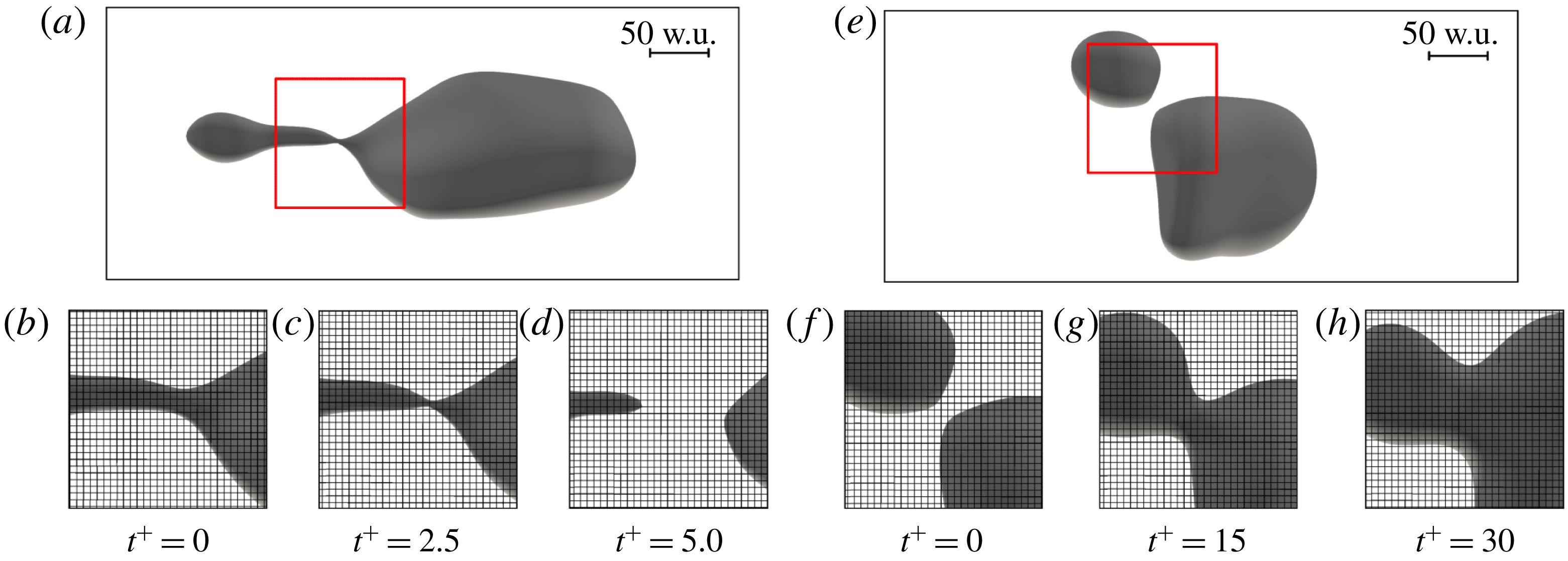
From the physical viewpoint, a breakage event can be divided into several stages (Notz & Basaran Reference Notz and Basaran2004). (i) Thread formation: the shear stresses stretch the droplet and a ligament is formed. (ii) Pinch-off: the thread elongates and capillary instabilities pinch off the ligament (neck formation). (iii) Thread breaking: the liquid thread breaks at the pinch-off and the newly formed droplets separate. Upon separation, surface tension reshapes the droplets and the threads are retracted. Overall, breakage is a very quick phenomenon that can be well approximated without resolving the dynamics at the molecular scale; there is evidence that the Navier–Stokes equations alone provide an adequate description of a breakage event (Eggers Reference Eggers1995). In addition, the small time scale of a breakage limits the impact of the approximation on the overall dynamics of the flow (Herrmann Reference Herrmann2011; Lu & Tryggvason Reference Lu and Tryggvason2018, Reference Lu and Tryggvason2019). Therefore, regardless of the methodology used, the description of breakages on turbulence-resolved grids is considered to be rather accurate, although in the pinch-off region the high curvature of the interface may not be perfectly resolved. Breakage events are implicitly described in interface-capturing methods (Hirt & Nichols Reference Hirt and Nichols1981; Jacqmin Reference Jacqmin1999; Sethian Reference Sethian1999), while interface-tracking methods require explicit extra efforts, which turn into the identification of suitable closure models to manage the connectivity of the marker points (Tryggvason et al. Reference Tryggvason, Bunner, Esmaeeli, Juric, Tauber, Han, Nas and Jan2001; Tryggvason, Scardovelli & Zaleski Reference Tryggvason, Scardovelli and Zaleski2011). In figure 2(a–d) we report the current numerical simulation of a breakage event, together with the computational grid and the length scale in wall units. In figure 2(b–d) the different stages of the breakage are reported with the running time of the simulation. Although the grid resolution is sufficient to resolve the Kolmogorov length scale of the turbulent flow (see § 2.5) and corresponds to a considerable computational effort, it is clear from the time sequence that the physical phenomena occur at length scales smaller than the grid resolution. As discussed before, however, the breakage occurs on a very short time scale (see figure 2 c,d), so that we expect a rather good numerical representation of this phenomenon.
Time sequence of a breakage event (b–d) and of a coalescence event (f–h). The breakage refers to the droplet reported in (a) while the coalescence refers to the droplets reported in (e). Time increases from left to right; the snapshots referring to the breakage event are captured every
 $\unicode[STIX]{x0394}t^{+}=2.5$
while those referring to the coalescence event every
 $\unicode[STIX]{x0394}t^{+}=15$
. Panels show a small portion of the domain in the
 $x$
–
 $y$
plane. Considering the breakage event, the thin thread becomes progressively thinner (b,c) and subsequently breaks (e). Conversely, considering the coalescence event, after the initial approach (f), the thin liquid film drains, a bridge is formed and the two droplets merge (g); finally surface tension forces reshape the droplet (h). As a reference, the computational grid employed (which has a spacing
 $\unicode[STIX]{x0394}x^{+}=3.68$
wall units (w.u.) and
 $\unicode[STIX]{x0394}y^{+}=3.68$
w.u.) is also reported. A red box (a,e) identifies the region of the domain reported in the smaller panels (b–d,f–h).

The dynamics of a coalescence event is more complex compared to that of a breakage. It is influenced by phenomena occurring at very small length scales (order of the molecular scale) and it occurs on larger time scales. From the physical viewpoint, the coalescence process can be divided into the following stages (Kamp, Villwock & Kraume Reference Kamp, Villwock and Kraume2017). (i) Approach: the two droplets approach each other. (ii) drainage: the thin liquid film between the droplets starts to drain. (iii) Coalescence: small-scale interactions lead to the rupture of the thin liquid film and to the formation of a coalescence bridge. (iv) Reshaping: surface tension forces reshape the droplet. Considering the small scales involved in film drainage and rupture, the description of a coalescence event in numerical simulations is extremely challenging. In addition, the physical mechanisms driving film rupture are still being investigated (Chen et al. Reference Chen, Kuhl, Tadmor, Lin and Israelachvili2004; Rekvig & Frenkel Reference Rekvig and Frenkel2007; Sreehari et al. Reference Sreehari, Borg, Chubynsky, Sprittles and Reese2019), and a correct prediction of the time required for film rupture cannot be explicitly obtained (Kamp et al. Reference Kamp, Villwock and Kraume2017). Therefore, a part of the physics involved in the coalescence process cannot be resolved or included in the two-phase flow numerical simulations. Current numerical simulations rely on different approaches to describe and/or model coalescence: closure models are required in interface-tracking methods (Tryggvason et al. Reference Tryggvason, Bunner, Esmaeeli, Juric, Tauber, Han, Nas and Jan2001; Lu & Tryggvason Reference Lu and Tryggvason2018, Reference Lu and Tryggvason2019), while coalescence is implicitly handled in interface-capturing methods, where two separate interfaces merge when they are closer than the grid resolution (Dodd & Ferrante Reference Dodd and Ferrante2016; Rosti, De Vita & Brandt Reference Rosti, De Vita and Brandt2019a ; Rosti et al. Reference Rosti, Ge, Jain, Dodd and Brandt2019b ). The current literature standpoint is that, regardless of the specific approach employed to describe coalescence, numerical simulations fail to describe physical coalescence, with this inaccuracy referred to as numerical coalescence. For all interface-capturing approaches, numerical coalescence over-predicts physical coalescence. Numerical coalescence for the interface-tracking methods depends on the parameters of the coalescence models used. Which is the best method to circumvent the issues produced by numerical coalescence is still debated: currently some numerical methods exploit film drainage models (Kwakkel, Breugem & Boersma Reference Kwakkel, Breugem and Boersma2013). These models, however, are based on strong simplifications (e.g. laminar flow of the film, flat or imposed interface shape, etc.), which might not be fully representative of the real configuration (Charles & Mason Reference Charles and Mason1960; Allan, Charles & Mason Reference Allan, Charles and Mason1961) and require the use of ad hoc tuned parameters. In figure 2(e–h) we report the numerical simulation of a coalescence event, together with the computational grid and the length scale in wall units. The different stages of the coalescence are reported with the simulation running time in figure 2(f–h). Considering the grid employed, it is clear that the approach (figure 2 f), the film drainage, the coalescence bridge formation (figure 2 g) and the reshaping (figure 2 h) stages can be accurately resolved, while film rupture (not shown here) is approximated on a much larger scale.
In the simulations presented in this work, we decided to maintain the method based on its thermodynamic foundations, without using any coalescence or breakage models. However, to examine the influence of numerical coalescence on the obtained results, we performed an assessment on a much finer grid with twice the number of points in all directions (i.e.
 $N_{x}\times N_{y}\times N_{z}=2048\times 1024\times 1025$
). The use of a refined grid allows for the use of a halved thickness of the thin interfacial transition layer (i.e. a halved Cahn number) and at the same time allows one to mitigate the effect of the numerical coalescence on the results obtained. A comparison of the results obtained on the two grids (coarse:
 $N_{x}\times N_{y}\times N_{z}=1024\times 512\times 513$
; fine:
 $N_{x}\times N_{y}\times N_{z}=2048\times 1024\times 1025$
) seems to suggest that it is possible to obtain fairly consistent results only slightly influenced by the grid resolution. This fairly good convergence of the results is achieved also because of the adoption a proper scaling between the mobility (Péclet number) and the thickness of the thin interfacial layer (Yue, Zhou & Feng Reference Yue, Zhou and Feng2010; Magaletti et al.
Reference Magaletti, Picano, Chinappi, Marino and Casciola2013). For the sake of a complete discussion of this point, we anticipate here some details of §§ 3.6 and 3.8. We find that coalescence and breakage rates obtained with the two grids differ by no more than 10 %; we also observe that the resulting DSDs almost overlap. The simulations here presented seem a fair approximation of the two-phase flow system from the macroscopic point of view (e.g. dispersed-phase morphology, coalescence and breakage rates, surfactant distribution). However, we ought to underline that a main shortcoming of these simulations – based on a continuum description of the system – is that the molecular-scale physics governing the drainage and rupture (Kamp et al.
Reference Kamp, Villwock and Kraume2017) cannot be simulated. Thus, these simulations cannot be used to extract microscopic information concerning film rupture and the role played by the surfactant molecules in such a process. Clearly, the importance of including the full physics (and the way in which it is modeled and included) cannot be estimated a priori on a quantitative basis, and this is still an important open research question.
2.4 Numerical method
The governing equations (2.1), (2.2)–(2.13) and (2.14) have been solved in a closed-channel geometry using a pseudo-spectral method (Hussaini & Zang Reference Hussaini and Zang1987; Canuto et al.
Reference Canuto, Hussaini, Quarteroni and Zang1988; Peyret Reference Peyret2002). In particular, the equations are discretized using Fourier series along the streamwise and spanwise directions (
 $x$
and
 $y$
) and Chebyshev polynomials along the wall-normal direction (
 $z$
). All the unknowns (velocity
 $\boldsymbol{u}$
, phase field
 $\unicode[STIX]{x1D719}$
and surfactant concentration
 $\unicode[STIX]{x1D713}$
) and their respective governing equations are Eulerian and are solved on the same Cartesian grid.
The governing equations are advanced in time using an implicit–explicit scheme. The linear diffusive term of the equations is integrated using an implicit scheme, while the nonlinear part is integrated using an explicit scheme. For the the Navier–Stokes equations, an Adams–Bashforth scheme is used for the nonlinear part while a Crank–Nicolson scheme is used for the linear term. For the Cahn–Hilliard-like equations, the nonlinear terms are time-discretized using an Adams–Bashforth algorithm while linear terms are discretized using an implicit Euler algorithm. The adoption of the implicit Euler scheme allows for the damping of unphysical high-frequency oscillations that could arise from the steep gradients present in the Cahn–Hilliard equations (Badalassi, Ceniceros & Banerjee Reference Badalassi, Ceniceros and Banerjee2003; Yue et al. Reference Yue, Feng, Liu and Shen2004).
In this scheme, the Navier–Stokes equations are not directly solved but are rewritten in the so-called velocity–vorticity formulation: instead of three second-order equations for each component of the velocity, a fourth-order equation for the wall-normal component of the velocity and a second-order equation for the wall-normal component of the vorticity
 $\unicode[STIX]{x1D714}_{z}$
are obtained (Kim, Moin & Moser Reference Kim, Moin and Moser1987; Speziale Reference Speziale1987). The phase field and the surfactant concentration transport equations are directly solved in their original formulation. Further details of the method can be found in Soligo et al. (Reference Soligo, Roccon and Soldati2019a
,Reference Soligo, Roccon and Soldati
b
).
The system of transport equations is completed by a set of suitable boundary conditions. For the Navier–Stokes equations a no-slip boundary condition is imposed at the two walls at
 $z=\pm 1$
:
 $$\begin{eqnarray}\boldsymbol{u}(z=\pm 1)=\mathbf{0}.\end{eqnarray}$$
For the phase field, the surfactant concentration and the respective chemical potentials, no-flux boundary conditions are enforced at the two walls. This is formally equivalent to imposing the following boundary conditions:
 $$\begin{eqnarray}\frac{\unicode[STIX]{x2202}\unicode[STIX]{x1D719}}{\unicode[STIX]{x2202}z}(z=\pm 1)=0,\quad \frac{\unicode[STIX]{x2202}^{3}\unicode[STIX]{x1D719}}{\unicode[STIX]{x2202}z^{3}}(z=\pm 1)=0,\quad \frac{\unicode[STIX]{x2202}\unicode[STIX]{x1D713}}{\unicode[STIX]{x2202}z}(z=\pm 1)=0.\end{eqnarray}$$
Along the streamwise and spanwise directions (
 $x$
and
 $y$
), periodic boundary conditions are implicitly imposed (Fourier discretization) on all variables. The adoption of these boundary conditions leads to the conservation of both phase field and surfactant concentration over time:
 $$\begin{eqnarray}\frac{\unicode[STIX]{x2202}}{\unicode[STIX]{x2202}t}\int _{\unicode[STIX]{x1D6FA}}\unicode[STIX]{x1D719}\,\text{d}\unicode[STIX]{x1D6FA}=0,\quad \frac{\unicode[STIX]{x2202}}{\unicode[STIX]{x2202}t}\int _{\unicode[STIX]{x1D6FA}}\unicode[STIX]{x1D713}\,\text{d}\unicode[STIX]{x1D6FA}=0.\end{eqnarray}$$
As a consequence, the total mass of the two phases and of the surfactant concentration is conserved. Despite this, mass conservation of each of the two phases,
 $\unicode[STIX]{x1D719}=+1$
and
 $\unicode[STIX]{x1D719}=-1$
, is not guaranteed (Yue et al.
Reference Yue, Zhou and Feng2007; Soligo et al.
Reference Soligo, Roccon and Soldati2019b
) and some small leakages between the phases may occur. In the cases presented here, because of the adoption of the profile-corrected formulation (Li et al.
Reference Li, Choi and Kim2016; Soligo et al.
Reference Soligo, Roccon and Soldati2019b
), mass leakages occur only during the initial transient; the total mass loss of the dispersed phase reaches at most 8 % in the worst case. This issue is linked with the initial condition adopted and will be discussed in more detail in the next section.
2.5 Simulation set-up
The computational domain is a closed channel with dimensions
 $L_{x}\times L_{y}\times L_{z}=4\unicode[STIX]{x03C0}h\times 2\unicode[STIX]{x03C0}h\times 2h$
corresponding to
 $L_{x}^{+}\times L_{y}^{+}\times L_{z}^{+}=3770\times 1885\times 600$
wall units (see appendix B for details on the wall units scaling). Equations are discretized on a grid with
 $N_{x}\times N_{y}\times N_{z}=1024\times 512\times 513$
collocation points. The simulations are performed at a fixed shear Reynolds number of
 $Re_{\unicode[STIX]{x1D70F}}=300$
. We consider two values of the surface tension, corresponding to
 $We=1.50$
and
 $We=3.00$
. The selected surface tension values match those commonly found in oil–water mixtures (Than et al.
Reference Than, Preziosi, Joseph and Arney1988). To analyse the effects introduced by the surfactant, for each surface tension value (Weber number), we test four different surfactants, characterized by increasing elasticity numbers (i.e. increasing surfactant strength). In particular, we consider the following elasticity numbers:
 $\unicode[STIX]{x1D6FD}_{s}=0.50$
(weaker surfactant),
 $\unicode[STIX]{x1D6FD}_{s}=1.00$
,
 $\unicode[STIX]{x1D6FD}_{s}=2.00$
and
 $\unicode[STIX]{x1D6FD}_{s}=4.00$
(stronger surfactant). In all these cases the total amount of surfactant is kept fixed (set with the surfactant bulk concentration,
 $\unicode[STIX]{x1D713}_{b}$
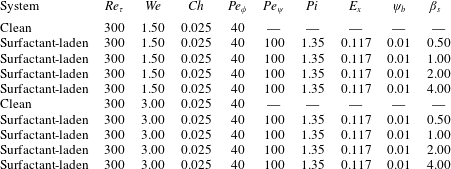
). Overall, we performed a total of 10 simulations: a clean system and four surfactant-laden systems for each Weber number; refer to table 1 for an overview of the parameters considered.
Summary of the parameters used for the different cases examined. For each Weber number, one clean (surfactant free) and four surfactant-laden systems have been considered. The surfactant-laden systems differ in the value of the elasticity number, which spans the range from
 $\unicode[STIX]{x1D6FD}_{s}=0.50$
(weaker surfactant) to
 $\unicode[STIX]{x1D6FD}_{s}=4.00$
(stronger surfactant).

The Cahn number has been set to
 $Ch=0.025$
: this value has been chosen according to the grid resolution as it allows for the accurate description of the steep gradients present at the interface. The phase field Péclet number,
 $Pe_{\unicode[STIX]{x1D719}}$
, has been set to
 $Pe_{\unicode[STIX]{x1D719}}=1/Ch=40$
, in order to respect the guidelines given in Yue et al. (Reference Yue, Zhou and Feng2010) and Magaletti et al. (Reference Magaletti, Picano, Chinappi, Marino and Casciola2013), which, for increasing grid resolutions, allows convergence to the sharp interface limit. The choice of these two parameters is crucial and, as will be discussed in § 3.8, the adoption of the scaling
 $Pe_{\unicode[STIX]{x1D719}}\propto Ch^{-1}$
guarantees the convergence of the results. Clearly, on increasing the grid resolution (and thus the computational cost), smaller Cahn numbers can be adopted and the dynamics of smaller droplets can be captured. However, the dynamics of the larger droplets (droplets large enough to be described with the current grid resolutions) is almost unchanged. Finally, the penalty flux parameter has been set to
 $\unicode[STIX]{x1D706}=2.5$
following the indications given by Li et al. (Reference Li, Choi and Kim2016) and Soligo et al. (Reference Soligo, Roccon and Soldati2019b
).
For the surfactant, the bulk concentration was kept fixed in all cases to
 $\unicode[STIX]{x1D713}_{b}=0.01$
. The Péclet number has been set to
 $Pe_{\unicode[STIX]{x1D713}}=100$
; this value can be considered representative of the behaviour of non-ionic and anionic surfactants in aqueous solutions (Weinheimer, Fennell & Cussler Reference Weinheimer, Fennell and Cussler1981). The temperature-dependent parameter has been set to
 $Pi=1.35$
and the surfactant solubility parameter to
 $E_{x}=0.117$
. These values have been set according to previous work of Engblom et al. (Reference Engblom, Do-Quang, Amberg and Tornberg2013). Despite these two parameters having a physical relevance, their effect is not investigated here for reasons of simplicity. However, it can be anticipated that for smaller
 $E_{x}$
and/or larger
 $Pi$
(stronger adsorption and diffusion), we expect a more uniform surfactant concentration due to enhanced diffusion.
At the beginning of the simulations, a regular array of 256 spherical droplets with diameter
 $d=0.4h$
(corresponding to
 $d^{+}=120$
wall units) is initialized in a fully developed turbulent channel flow; this flow field is obtained from a preliminary direct numerical simulation of a single-phase flow at
 $Re_{\unicode[STIX]{x1D70F}}=300$
. With this configuration, the dispersed-phase volume fraction
 $\unicode[STIX]{x1D6F7}=V_{d}/(V_{c}+V_{d})$
(
 $V_{d}$
and
 $V_{c}$
being the volume of the dispersed and carrier phases, respectively) is
 $\unicode[STIX]{x1D6F7}\simeq 5.4\,\%$
; the same volume fraction was used in previous works (Scarbolo et al.
Reference Scarbolo, Bianco and Soldati2015; Scarbolo, Bianco & Soldati Reference Scarbolo, Bianco and Soldati2016). The phase field and the surfactant concentration are initialized with their respective equilibrium profiles: the phase field is constant in the bulk of the phases (
 $\unicode[STIX]{x1D719}=+1$
in the droplets and
 $\unicode[STIX]{x1D719}=-1$
in the carrier fluid) and undergoes a smooth transition across the thin interfacial layer. Similarly, the surfactant concentration is uniform in the bulk of the two phases (
 $\unicode[STIX]{x1D713}=\unicode[STIX]{x1D713}_{b}$
) and reaches its peak value at the interface (
 $\unicode[STIX]{x1D713}=\unicode[STIX]{x1D713}_{0}$
). At the beginning of the simulation, turbulent fluctuations of the undisturbed flow field strongly perturb the phase-field interfacial profile, leading to a reduction of the mass of the dispersed phase. After this initial transient, during which the flow field and the phase field couple together, the mass of each phase remains constant over time.
Before proceeding, we justify the initial condition chosen for the phase field, which may seem unrealistic, since a swarm of spherical droplets is suddenly appearing in a single-phase flow field. To prove its consistency and to guarantee the independence of the results from the selected initial condition, we performed further preliminary simulations (not reported here) in which different initial conditions were considered, such as, for instance, the injection of a liquid sheet at the channel centre. All the different initial conditions tested achieve the same statistically steady results, indicating that memory of the initial condition is completely lost after an initial transient. In addition, the initial condition we chose requires a shorter time to reach a steady-state configuration with respect to the other initial conditions tested. For these reasons and to better compare our results with previous works (Scarbolo et al. Reference Scarbolo, Bianco and Soldati2015, Reference Scarbolo, Bianco and Soldati2016; Roccon et al. Reference Roccon, De Paoli, Zonta and Soldati2017), the presented initial condition (regular array of spherical droplets) has been employed here.
3 Results
We characterize the behaviour of the multiphase system from both qualitative and quantitative viewpoints so as to obtain a physically grounded understanding of the outcome of the competition among inertial forces, viscous forces and surface tension forces. After describing on a qualitative basis the steady state of the system, for each of the examined cases we characterize the surfactant concentration over the droplet interface by computing its probability density function (PDF) and by studying the influence of the droplet size on its distribution. Then, we focus on the modifications produced by the surfactant dynamics on the dispersed phase morphology, which we characterize using macroscopic indicators, such as the number of droplets and their breakage and coalescence rates. Finally, we analyse the resulting DSD and we compare it with the theoretical scaling developed by Garrett, Li & Farmer (Reference Garrett, Li and Farmer2000). A detailed description of turbulence modifications produced by the presence of a swarm of droplets is beyond the scope of this work and will be investigated in the future. However, we can anticipate that, as reported in previous works (Scarbolo et al.
Reference Scarbolo, Bianco and Soldati2016; Roccon et al.
Reference Roccon, De Paoli, Zonta and Soldati2017), a slight increase of the flow rate (
 $\simeq 1\,\%$
) is observed for all cases considered (simulations are performed with a constant pressure gradient driving the flow).
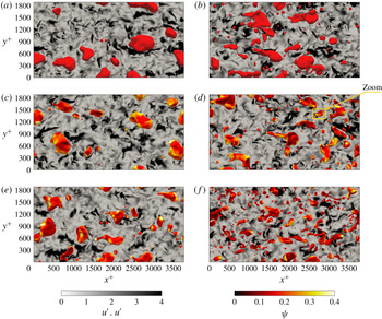
Top view of the steady-state configuration (
 $t^{+}=3750$
) attained by six different cases: (a,c,e)
 $We=1.50$
; (b,d,f)
 $We=3.00$
. (a,b) Clean cases; (c,d)
 $\unicode[STIX]{x1D6FD}_{s}=1.00$
; (e,f)
 $\unicode[STIX]{x1D6FD}_{s}=4.00$
. In each panel, the interface of the droplets (iso-contour
 $\unicode[STIX]{x1D719}=0$
) is coloured in red for the clean cases (a,b) and by the surfactant concentration for the surfactant-laden cases (c–f): red identifies regions with a low concentration, while white identifies regions with a high concentration. In the background, an
 $x^{+}$
–
 $y^{+}$
plane located at
 $z^{+}=0$
(centre of the channel) shows the magnitude of the velocity fluctuations,
 $\boldsymbol{u}^{\prime }\boldsymbol{\cdot }\boldsymbol{u}^{\prime }$
. In (d), a yellow box highlights the sample droplet used in the following to present the interaction between shear stresses and Marangoni stresses (see figure 5).

3.1 Qualitative behaviour of multiphase flow
After the release of the droplets in the turbulent channel flow (
 $t^{+}=0$
), each single droplet starts to interact with the background turbulence and with the neighbouring droplets. In this initial transient, droplets are deformed by the action of the shear stress, and coalescence and breakage phenomena start to take place. At the same time, surfactant is redistributed according to the local flow field and to the dispersed phase morphology (number and shape of the droplets). After this transient, memory of the initial condition is lost and the multiphase flow reaches a statistically steady configuration. This new configuration is shown in figure 3 for six different combinations of the parameters at
 $t^{+}=3750$
. Panel (a,c,e) refers to
 $We=1.50$
and (b,d,f) to
 $We=3.00$
. Each row corresponds to a different elasticity number: clean (a,b),
 $\unicode[STIX]{x1D6FD}_{s}=1.00$
(c,d) and
 $\unicode[STIX]{x1D6FD}_{s}=4.00$
(e,f). The system configuration is displayed showing all the droplets in the top half of the channel, identified by the iso-contour
 $\unicode[STIX]{x1D719}=0$
(interface); for the surfactant-laden cases (c–f), the interface is coloured by the surfactant concentration. In addition, to give a qualitative overview of the modifications induced in the carrier fluid turbulence by the dispersed phase, the magnitude of the velocity fluctuations,
 $\boldsymbol{u}^{\prime }\boldsymbol{\cdot }\boldsymbol{u}^{\prime }$
, on an
 $x^{+}$
–
 $y^{+}$
plane located at the channel centre (
 $z^{+}=0$
) is reported in greyscale (white, low; black, high).
From these qualitative pictures, we can make two important observations: the different combinations of the Weber and elasticity numbers have a strong impact on the dispersed-phase morphology and the surfactant distribution over the interface of the droplets is non-uniform. In particular, analysing the surfactant concentration, we observe that larger droplets exhibit a highly non-uniform surfactant distribution while for smaller droplets the distribution tends to be more uniform. In addition, we observe also the presence of small regions that exhibit high surfactant concentrations (bright yellow/white regions). Turning to the dispersed-phase morphology, we can clearly notice the effect of the Weber and elasticity numbers. Specifically, for both Weber numbers, an increase of the elasticity number leads to the formation of smaller droplets and to the consequent increase of the number of droplets and of the total interfacial area. The typical droplet size reduces as either the elasticity number or the Weber number is increased: a reduction of the surface tension weakens surface tension forces and promotes larger curvature values and, eventually, droplet breakage. Finally, we can observe some qualitative differences from the map of the velocity fluctuation magnitude: for
 $We=1.50$
(a,c,e), regions characterized by large velocity fluctuations are more elongated and cover a significant area, while for
 $We=3.00$
(b,d,f) these regions are smaller and more fragmented. This difference can be better appreciated comparing the two extreme cases: figures 3(a) and 3(f).
3.2 Shear stresses, Marangoni stresses and breakage/coalescence of droplets
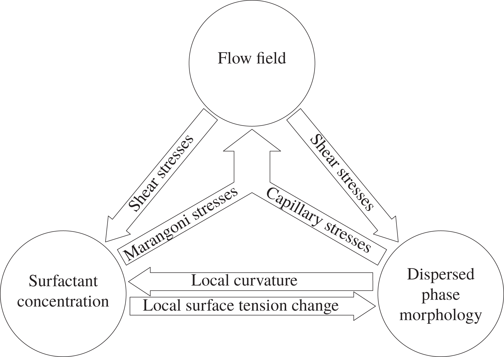
Before proceeding with a more quantitative characterization of the results, it is worth briefly describing the complex interactions among the flow, the interface and the local surfactant concentration. These interactions, which are graphically summarized in figure 4, are deeply interconnected and the contribution of each single factor (flow, interface and surfactant) cannot be disentangled easily. We start by considering the action of the turbulent flow on the phase field (dispersed-phase morphology) and on the surfactant concentration. The turbulent flow, with the associated shear stresses, transports surfactant over the interface, depleting some regions of surfactant and accumulating it in others (top to bottom-left arrow). In addition, the shear stresses directly influence the dispersed phase morphology: strong shear stresses deform the interface and promote breakage of the droplets (top to bottom-right arrow). In turn, the surfactant-laden interface generates stresses according to the local dispersed-phase morphology and surfactant concentration (bottom to top arrows). These stresses modify the local flow field and shear stresses, which in turn affect the merging, breaking and stretching of the interface and the surfactant distribution. For instance, Marangoni stresses (tangential to the interface) help in preventing coalescence, since they hinder the drainage of the liquid film separating the droplets (Dai & Leal Reference Dai and Leal2008; Soligo et al. Reference Soligo, Roccon and Soldati2019a ). In a similar way, the modifications of the local flow field produced by Marangoni stresses are crucial in the breakage of droplets (Stone & Leal Reference Stone and Leal1990) and in the pinch-off of liquid threads (Kamat et al. Reference Kamat, Wagoner, Thete and Basaran2018).
Graphical representation of the main interactions among flow field, dispersed-phase morphology and surfactant concentration. On the one hand, the shear stresses produced by the flow field affect the dispersed-phase morphology and the surfactant distribution (top to bottom arrows). On the other hand, capillary and Marangoni stresses influence the local flow field (bottom to top arrows). Then, also the dispersed-phase morphology and the surfactant concentration mutually interact: the surfactant distribution locally reduces surface tension and increases the interface deformability (left to right arrow). This effect is reflected in the interface morphology and dynamics, which in turn affect the surfactant distribution (right to left arrow).

The surfactant distribution and the dispersed-phase morphology are closely linked together. In particular, the interface deformation (stretching and compression) favours the accumulation or dilution of surfactant and thus leads to a change in the local surfactant concentration (right to left arrow). In addition, the interface curvature influences the adsorption of surfactant from the bulk towards the interface and vice versa (Hsu, Chang & Lin Reference Hsu, Chang and Lin2000; Eggleton, Tsai & Stebe Reference Eggleton, Tsai and Stebe2001). The resulting surfactant distribution, in turn, influences the local curvature: surfactant increases the interface deformability (lower surface tension) and, as a consequence, large curvature values are favoured by high surfactant concentrations (left to right arrow).
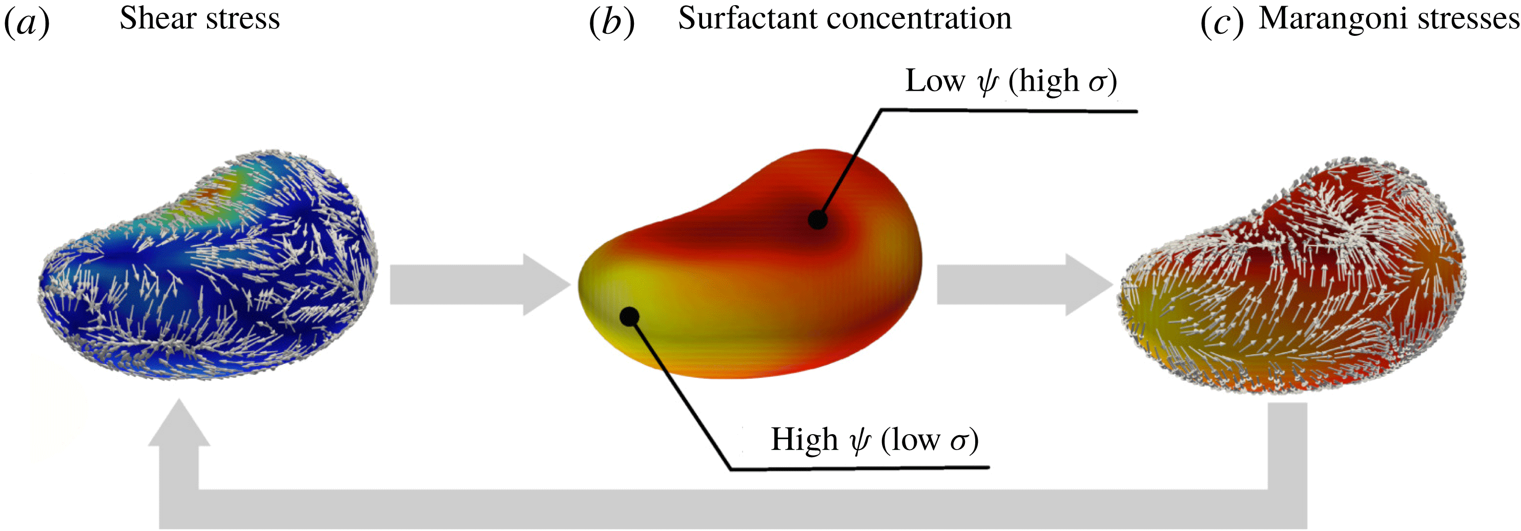
Sketch of the coupling between shear and Marangoni stresses. The sketch is realized considering the droplet marked by the yellow box in figure 3(d). (a) The component tangential to the interface of the shear stresses,
 $\boldsymbol{S}_{t}$
, on the droplet interface and normalized by its magnitude (see appendix C for details of
 $\boldsymbol{S}_{t}$
). The interface is coloured by the shear stress magnitudes (blue, small; red, large). (b) The resulting non-uniform surfactant distribution (red, low; yellow, high). This distribution, in turn, leads to a non-uniform surface tension distribution and thus gives rise to Marangoni stresses, shown in (c) using unit length vectors. These stresses try to restore a uniform value of the surface tension, driving flow from regions of high surfactant concentration (yellow) towards regions with a lower concentration (red). The Marangoni stresses feed back to the local shear stress distribution (right to left arrow).

We now focus on the main factors determining the surfactant concentration over the interface of the droplets: an interesting coupling between shear and Marangoni stresses can be highlighted. This coupling is explained using figure 5, which shows the shear stresses (figure 5
a), the surfactant concentration (figure 5
b) and Marangoni stresses (figure 5
c) on the interface of the sample droplet marked by a yellow rectangle in figure 3(d). First, we consider the shear stresses; their action, in conjunction with the droplet shape, leads to a non-uniform surfactant distribution. This first interaction can be appreciated by looking at figure 5(a,b), showing the component tangential to the interface of the shear stresses,
 $\boldsymbol{S}_{t}$
, normalized by its magnitude (reported only on the interface, blue, small; red, large), and showing the surfactant distribution on the droplet interface (red, low; yellow, high). The resulting non-uniform surfactant distribution generates a non-uniform surface tension which, in turn, gives rise to Marangoni stresses, which are tangential to the interface and act to restore a uniform value of the surface tension by sweeping surfactant from high-concentration regions (low surface tension, yellow) towards low-concentration regions (high surface tension, red). Marangoni stresses are proportional to the surface tension gradient and can be directly linked to the surfactant concentration via the surface tension EOS. Their action is shown in figure 5(c), which reports the spatial distribution of Marangoni stresses (normalized by their magnitude) on the droplet interface (coloured as in figure 5
b). It is interesting to observe that Marangoni stresses oppose the shear stresses (which generate a non-uniform surfactant distribution) and, therefore, lead to a reduction of the shear stresses at the droplet interface (right to left arrow).
3.3 Probability density function of interfacial surfactant concentration
To quantify the outcome of the interaction among flow field, dispersed-phase morphology and surfactant concentration, we start by analysing the surfactant distribution over the interface of the droplets. As suggested by figure 4, the distribution of the surfactant is determined by the interplay between local shear stresses, Marangoni stresses, dispersed-phase morphology and adsorption/desorption phenomena. To quantify the outcome, we compute the PDF of the interfacial surfactant concentration (i.e. the surfactant concentration at the interface, identified as the iso-contour
 $\unicode[STIX]{x1D719}=0$
). The results, computed once a steady configuration is obtained (from
 $t^{+}>2500$
until the end of the simulation), are reported in figure 6 for
 $We=1.50$
and
 $We=3.00$
.
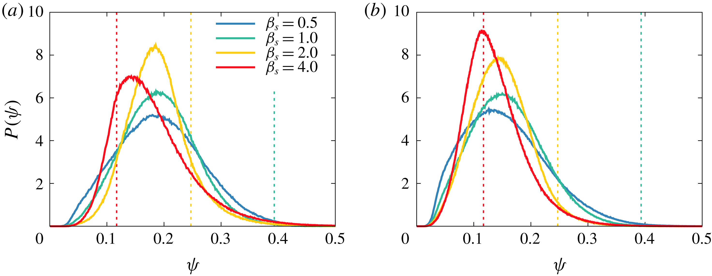
The PDF of the interfacial surfactant concentration: (a)
 $We=1.50$
; (b)
 $We=3.00$
. The different colours refer to
 $\unicode[STIX]{x1D6FD}_{s}=0.50$
(blue),
 $\unicode[STIX]{x1D6FD}_{s}=1.00$
(green),
 $\unicode[STIX]{x1D6FD}_{s}=2.00$
(yellow) and
 $\unicode[STIX]{x1D6FD}_{s}=4.00$
(red). The concentration at which the shutdown of Marangoni stresses occurs (shutdown concentration,
 $\unicode[STIX]{x1D713}_{s}$
) is reported with thin dashed lines (same colours as before). In general, for higher elasticity numbers, the PDF becomes taller and narrows around the most probable value. However, for the cases at
 $\unicode[STIX]{x1D6FD}_{s}=4.00$
, the shutdown of Marangoni stresses markedly affects the PDF shape. This modification is particularly evident for
 $\unicode[STIX]{x1D6FD}_{s}=4.00$
and
 $We=1.50$
, the red line in (a).

For
 $We=1.50$
(figure 6
a), the PDFs are asymmetric and skewed to the right: stronger positive fluctuations in the surfactant concentration are more likely to occur, while strong negative fluctuations rarely happen. The asymmetry present in the PDF shape becomes more pronounced as the elasticity number increases. In addition, we observe that the mean value of the interfacial surfactant concentration shifts towards smaller values for larger elasticity numbers. This shift can be traced back to the increase of the total interfacial area, which is originated by a larger number of droplets with a more deformable interface. This effect is more pronounced for stronger surfactants (higher elasticity numbers), which indeed are more effective in reducing surface tension. Since surfactant distributes over the droplet interface, a larger interface extension reduces the average surfactant concentration.
We now focus on the three lower elasticity numbers (
 $\unicode[STIX]{x1D6FD}_{s}=0.50$
,
 $\unicode[STIX]{x1D6FD}_{s}=1.00$
and
 $\unicode[STIX]{x1D6FD}_{s}=2.00$
); the case for
 $\unicode[STIX]{x1D6FD}_{s}=4.00$
requires a specific consideration and will be discussed later on. For these three cases, we can clearly notice that the PDF narrows about its peak as the elasticity number is increased. This effect originates from the action of the Marangoni stresses, which act to restore a uniform value of the surface tension and whose amplitude is proportional to the elasticity number. Indeed, Marangoni stresses favour a uniform surfactant distribution, as reflected by the narrowing of the surfactant concentration about its peak. In addition, we can also observe that low values of the surfactant concentration are strongly penalized: the surfactant concentration is strictly bounded in
 $\unicode[STIX]{x1D713}=(0,1)$
, as prescribed by the chemical potential (equation (2.8)). Turning now to the highest elasticity number (
 $\unicode[STIX]{x1D6FD}_{s}=4.00$
), the PDF exhibits a markedly different behaviour: the most probable value of the PDF is lower (with respect to
 $\unicode[STIX]{x1D6FD}_{s}=2.00$
) and the shape is more right-skewed. The origin of this behaviour is connected to the shutdown of Marangoni stresses. Indeed, the maximum surface tension reduction is bounded and once the surfactant concentration is higher than a critical value, here referred to as shutdown concentration
 $\unicode[STIX]{x1D713}_{s}$
, surface tension remains constant and the action of Marangoni stresses ceases. The shutdown concentration,
 $\unicode[STIX]{x1D713}_{s}$
, can be computed from the surface tension EOS by imposing
 $f_{\unicode[STIX]{x1D70E}}(\unicode[STIX]{x1D713}_{s})=0.5$
:
 $$\begin{eqnarray}\unicode[STIX]{x1D713}_{s}(\unicode[STIX]{x1D6FD}_{s})=1-\text{e}^{-0.5/\unicode[STIX]{x1D6FD}_{s}}.\end{eqnarray}$$
The resulting shutdown concentrations (
 $\unicode[STIX]{x1D713}_{s}=0.117$
for
 $\unicode[STIX]{x1D6FD}_{s}=4.00$
,
 $\unicode[STIX]{x1D713}_{s}=0.221$
for
 $\unicode[STIX]{x1D6FD}_{s}=2.00$
and
 $\unicode[STIX]{x1D713}_{s}=0.393$
for
 $\unicode[STIX]{x1D6FD}_{s}=1.00$
) are reported in figure 6 with thin dashed vertical lines with colours corresponding to the PDF data. The shutdown concentration for
 $\unicode[STIX]{x1D6FD}_{s}=0.50$
(
 $\unicode[STIX]{x1D713}_{s}=0.632$
) is not shown since it exceeds the plot limits. As can be appreciated from figure 6(a), the shutdown affects only marginally the PDF shape for
 $\unicode[STIX]{x1D6FD}_{s}=2.00$
(and for lower
 $\unicode[STIX]{x1D6FD}_{s}$
), while a more pronounced effect is observed for
 $\unicode[STIX]{x1D6FD}_{s}=4.00$
. For this latter case, the shutdown occurs at concentrations lower than the most probable value. Therefore, surface tension is constant for
 $\unicode[STIX]{x1D713}\geqslant 0.117$
and Marangoni stresses vanish, thus eliminating their feedback action on the shear stresses; this results in a wider and more asymmetric PDF. Finally, we can observe that the most probable value for the case
 $\unicode[STIX]{x1D6FD}_{s}=4.00$
is shifted towards lower concentrations. This shift originates from the higher number of droplets (larger interfacial area) attained by this latter case (see also § 3.5 for a detailed characterization of the number of droplets).
For
 $We=3.00$
(figure 6
b), the PDF of the surfactant concentration follows a monotonic trend: large fluctuations in the surfactant concentration are less frequent and the most probable value shifts towards lower concentrations for larger elasticity numbers. These two observations directly reflect the action of Marangoni stresses, which favour a more uniform surfactant concentration. Interestingly, for the cases here considered (
 $We=3.00$
), the shutdown of Marangoni stresses has a minor impact on the shape of the PDF. Indeed, the higher Weber number (lower clean reference surface tension) leads to a much larger total interfacial area, and thus the average concentration is lower. As a consequence, the resulting PDFs of these latter cases are shifted towards lower concentrations and a smaller portion of the PDF is influenced by the shutdown of Marangoni stresses. This minor impact of the shutdown is clearly reflected in the PDFs: as the elasticity number is increased, the PDFs narrow and the amplitude of the PDF peak continuously increases. However, for the highest elasticity number (
 $\unicode[STIX]{x1D6FD}_{s}=4.00$
), the effect of the shutdown is still visible and the respective PDF is strongly skewed to the right. Indeed, for this latter case, the shutdown concentration,
 $\unicode[STIX]{x1D713}_{s}=0.117$
, is slightly larger than the peak of the PDF. Therefore, only the part located to the right of the PDF peak is influenced by the shutdown. Finally, we can observe that for the two lower
 $\unicode[STIX]{x1D6FD}_{s}$
values, the boundedness of the surfactant concentration (
 $\unicode[STIX]{x1D713}>0$
) penalizes large negative fluctuations and affects the left tail of the distribution. This results in a more asymmetric PDF, especially for the lower elasticity numbers, as the PDF is wider (weaker restoring effect of Marangoni stresses) and shifted towards lower concentrations (larger interfacial area).
3.4 Droplet size influence on the interfacial surfactant concentration
In this subsection the influence of the droplet size on the surfactant distribution over the interface is investigated. In particular, we aim at quantifying the correlation between droplet size and surfactant concentration previously observed qualitatively in figure 3. For this purpose, the PDF of the surfactant concentration over the interface has been calculated separately for each droplet and then sorted depending on the droplet size. For each droplet, we compute the equivalent diameter,
 $d_{eq}^{+}$
, as the diameter of an equivalent spherical droplet with the same volume as the droplet considered:
 $$\begin{eqnarray}d_{eq}^{+}=\left(\frac{6V^{+}}{\unicode[STIX]{x03C0}}\right)^{1/3},\end{eqnarray}$$
where
 $V^{+}$
is the volume of the droplet.
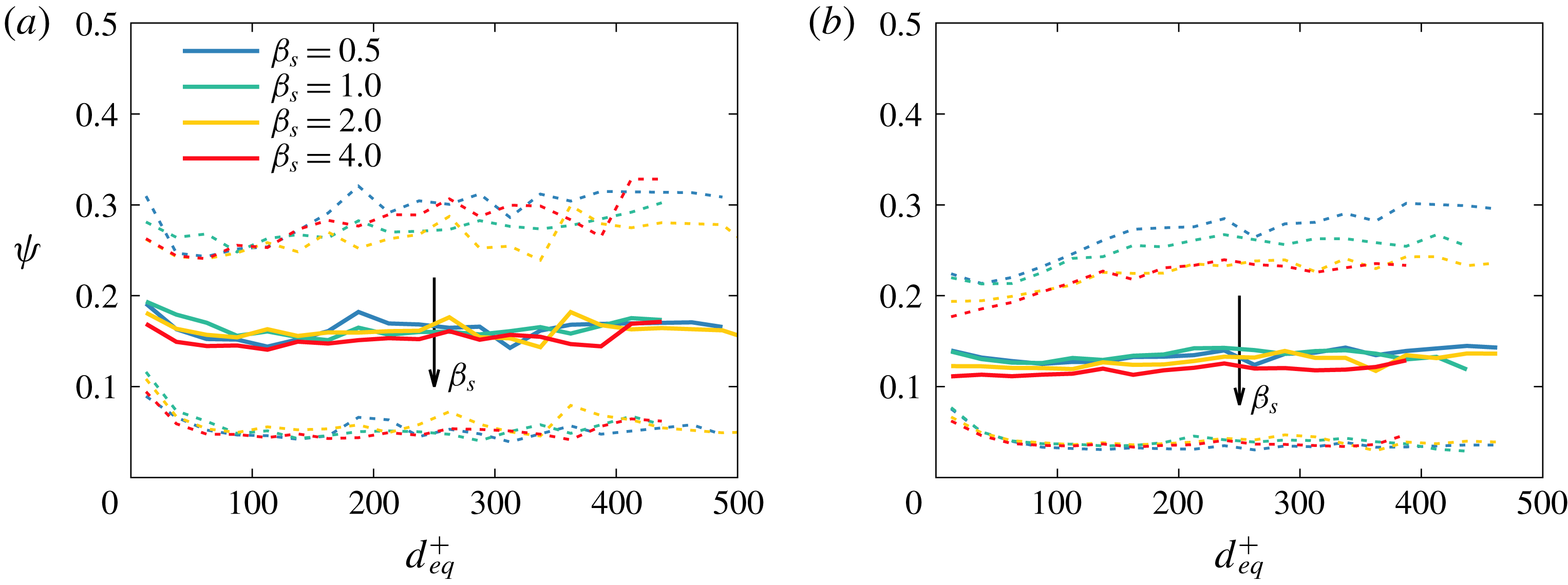
For the sake of clarity, only the mean value and the 5th and 95th percentiles of the surfactant concentration over the droplet interface are reported in figure 7; solid lines identify the mean value, while dashed lines correspond to the percentiles (
 $5\text{th}$
percentile below the mean value and 95th percentile above the mean value). The usual colour scheme is adopted to distinguish among the various cases:
 $\unicode[STIX]{x1D6FD}_{s}=0.50$
(blue),
 $\unicode[STIX]{x1D6FD}_{s}=1.00$
(green),
 $\unicode[STIX]{x1D6FD}_{s}=2.00$
(yellow) and
 $\unicode[STIX]{x1D6FD}_{s}=4.00$
(red). We start by analysing the results obtained for
 $We=1.50$
(figure 7
a). First, we notice that for all cases the mean surfactant concentration on the interface is not significantly influenced by droplet size. This indicates that the mixing effect induced by the coalescence and breakage events promotes a uniform surfactant distribution over the entire range of droplet sizes. Second, we observe that for higher elasticity numbers, the mean surfactant concentration on the interface is slightly reduced. This result is in agreement with our previous observation for the PDF of the surfactant concentration (figure 6): the lower surface tension (stronger surfactant) increases the total interfacial area, thus reducing the average surfactant concentration over the interface.
Influence of droplet size on surfactant concentration at the interface; thick solid lines represent the mean surfactant concentration, while dashed lines represent the
 $5\text{th}$
and
 $95\text{th}$
percentiles: (a)
 $We=1.50$
; (b)
 $We=3.00$
. The different cases are marked with different colours:
 $\unicode[STIX]{x1D6FD}_{s}=0.50$
(blue),
 $\unicode[STIX]{x1D6FD}_{s}=1.00$
(green),
 $\unicode[STIX]{x1D6FD}_{s}=2.00$
(yellow) and
 $\unicode[STIX]{x1D6FD}_{s}=4.00$
(red). The mean concentration is almost constant and is not affected by the droplet size; conversely, the droplet size has an influence on the fluctuations in the surfactant concentration (as indicated by the percentile lines) and smaller droplets exhibit a more uniform concentration. This effect originates from Marangoni stresses, which are more effective on smaller droplets (smaller length scale).

While the droplet size does not change the mean concentration of surfactant over the interface, a clear effect of the droplet size on the surfactant concentration fluctuations can be appreciated: the
 $5\text{th}$
and
 $95\text{th}$
percentile lines are closer to the mean value for smaller droplets. This means that smaller droplets have a more uniform surfactant distribution over their interface with respect to larger droplets. This effect can be traced back to Marangoni stresses, the magnitude of which is proportional to the surface tension gradient. The surface tension gradient can be approximated as the ratio of the surface tension variation,
 $\unicode[STIX]{x0394}\unicode[STIX]{x1D70E}$
, over the droplet equivalent diameter, here used as a characteristic length scale of the droplet. The magnitude of the surface tension variation,
 $\unicode[STIX]{x0394}\unicode[STIX]{x1D70E}$
, is of the same order of magnitude for all the droplet sizes (roughly similar to the difference between the
 $5\text{th}$
and the
 $95\text{th}$
percentiles). Hence, the action of Marangoni stresses (which act to restore a uniform surfactant distribution) is more effective on smaller droplets, as they are characterized by a lower equivalent diameter. It is important to note that, for the higher elasticity number considered here (
 $\unicode[STIX]{x1D6FD}_{s}=4.00$
), the shutdown of Marangoni stresses has a marked effect on the positive fluctuations in the surfactant concentration: as Marangoni stresses vanish (surface tension is constant for surfactant concentrations above the shutdown concentration), their restoring effect on the surfactant distribution ceases. Indeed, the trend of the
 $95\text{th}$
percentile line is lost for the stronger surfactant (
 $\unicode[STIX]{x1D6FD}_{s}=4.00$
), which is superposed to the
 $95\text{th}$
percentile line of the case at
 $\unicode[STIX]{x1D6FD}_{s}=2.00$
. Considering the
 $5\text{th}$
percentile lines, a similar trend can be observed among all the cases; this trend is particularly marked for larger droplets,
 $d_{eq}^{+}>100$
. This effect arises from the surfactant chemical potential, which strictly bounds the surfactant concentration between 0 and 1: thus, extremely low values of surfactant concentration are energetically unfavourable (high chemical potential) and strong negative fluctuations are hindered.
The effect of the droplet size on the surfactant distribution becomes more pronounced for
 $We=3.00$
(figure 7
b). A decrease in the mean surfactant concentration is observed for increasing elasticity numbers: the same total amount of surfactant distributes over a larger surface (higher interfacial area). As observed for
 $We=1.50$
(figure 7
a), the mean surfactant concentration does not depend on the droplet size, while the amplitude of the fluctuations increases with the droplet size. In particular, a clear trend is observed for the
 $95\text{th}$
percentile: as the elasticity number increases, Marangoni stresses become stronger and extreme values of surfactant concentration are less likely to occur. Due to the shutdown of Marangoni stresses, this trend is not observed between the cases with
 $\unicode[STIX]{x1D6FD}_{s}=2.00$
and
 $\unicode[STIX]{x1D6FD}_{s}=4.00$
: for this latter case surface tension remains constant above the shutdown concentration (
 $\unicode[STIX]{x1D713}_{s}=0.117$
) and, consequently, the action of Marangoni stresses vanishes. As the equilibrium-restoring effect of Marangoni stresses is partially lost, similar positive fluctuations of the surfactant concentration are observed for the two stronger surfactants (
 $\unicode[STIX]{x1D6FD}_{s}=2.00$
and
 $\unicode[STIX]{x1D6FD}_{s}=4.00$
). Also for these cases, the boundedness of the surfactant chemical potential (which prevents large negative fluctuations of the surfactant concentration) leads to a very similar behaviour for all the
 $5\text{th}$
percentile lines.
3.5 Time evolution of the number of droplets
The distribution of the surfactant over the droplet interface has direct consequences for the dispersed-phase morphology. In fact, the presence of surfactant produces a local decrease of surface tension (whose amplitude depends on the local surfactant concentration) and introduces Marangoni stresses, thus affecting the dynamics of coalescence and breakage events and the resulting dispersed-phase morphology (Dai & Leal Reference Dai and Leal2008; Takagi & Matsumoto Reference Takagi and Matsumoto2011; Liu et al.
Reference Liu, Ba, Wu, Li, Xi and Zhang2018). With the aim of characterizing the dispersed-phase morphology and of quantifying the previous qualitative observations (figure 3), we compute the time evolution of the number of droplets,
 $N(t^{+})$
. The results, normalized by the initial number of droplets
 $N_{0}=256$
(same for all the cases), are shown in figure 8.
Time evolution of the normalized number of droplets,
 $N(t^{+})/N_{0}$
: (a)
 $We=1.50$
; (b)
 $We=3.00$
. Different colours distinguish the various cases: clean (black),
 $\unicode[STIX]{x1D6FD}_{s}=0.50$
(blue),
 $\unicode[STIX]{x1D6FD}_{s}=1.00$
(green),
 $\unicode[STIX]{x1D6FD}_{s}=2.00$
(yellow) and
 $\unicode[STIX]{x1D6FD}_{s}=4.00$
(red). The action of surfactant can be clearly observed: on increasing the elasticity number
 $\unicode[STIX]{x1D6FD}_{s}$
, the surface tension reduction is larger and a greater number of droplets is found in the channel. For the cases at
 $We=1.50$
, this effect can be better appreciated from the inset of (a).

We start the discussion with the low-Weber-number cases (figure 8
a). During the initial stages of the simulation, all cases evolve in a similar manner: the total number of droplets decreases down to about 40 % of the initial value. Then, the five cases start to depart from each other: the effect of surfactant and of its strength is clearly reflected in the number of droplets. The clean and weak surfactant cases show a faster decrease in the number of droplets with respect to the strong surfactant cases. Finally, at
 $t^{+}\simeq 2500$
, a steady state for the number of droplets is reached indicating that coalescence and breakage events balance out. The effect of surface tension on the steady-state number of droplets is clear: the clean case has the lowest number of droplets at the end of the simulation. As the elasticity number is increased, also the final number of droplets increases. On average stronger surfactants are able to produce a greater number of smaller droplets in the channel. The different number of droplets attained at steady state can be linked to the maximum stable diameter (Hinze Reference Hinze1955), which is determined by the competition between stabilizing effects (e.g. surface tension) and destabilizing effects (e.g. turbulent fluctuations). Decreasing the average surface tension over the interface (stronger surfactant) leads to a reduction in the maximum stable diameter, thus to the formation of smaller droplets. The effect of surfactant can be better appreciated from the inset of figure 8(a), which shows the time evolution of the number of droplets at steady state. With respect to the clean case, the final number of droplets is increased by a factor ranging from
 $1.32$
(
 $\unicode[STIX]{x1D6FD}_{s}=0.50$
) up to
 $3.32$
(
 $\unicode[STIX]{x1D6FD}_{s}=4.00$
).
A markedly different behaviour is observed for the cases at
 $We=3.00$
(figure 8
b): after an initial decrease (up to
 $t^{+}=300$
) in the number of droplets for all cases, a marked increase is observed for the stronger surfactant cases. For these cases breakage events outnumber coalescence events, thus increasing the total number of droplets. After the initial transient stage, at about
 $t^{+}=2500$
, the number of droplets reaches a statistically steady-state value, which increases with the surfactant strength. In particular, the number of droplets in the clean and weak surfactant cases (
 $\unicode[STIX]{x1D6FD}_{s}=0.50$
and
 $\unicode[STIX]{x1D6FD}_{s}=1.00$
) reaches a steady-state value
 $N(t^{+})\simeq 0.5N_{0}$
, while for the stronger surfactant (
 $\unicode[STIX]{x1D6FD}_{s}=4.00$
) it reaches about
 $N(t^{+})\simeq 1.5N_{0}$
. With respect to the clean case, the steady-state number of droplets is increased by a factor ranging from
 $1.18$
(
 $\unicode[STIX]{x1D6FD}_{s}=0.50$
) to
 $3.16$
(
 $\unicode[STIX]{x1D6FD}_{s}=4.00$
). It is interesting to observe that although the steady-state number of droplets strongly differs between the two Weber numbers, ranging between 19 (clean case) and 63 (
 $\unicode[STIX]{x1D6FD}_{s}=4.00$
) for
 $We=1.50$
and between 116 (clean case) and 366 (
 $\unicode[STIX]{x1D6FD}_{s}=4.00$
) for
 $We=3.00$
, the increase in the number of droplets with respect to the clean reference cases is similar: from a factor of about
 $1.25$
for the weakest surfactant (
 $\unicode[STIX]{x1D6FD}_{s}=0.50$
) up to about
 $3.25$
for the strongest one (
 $\unicode[STIX]{x1D6FD}_{s}=4.00$
).
3.6 Coalescence and breakage rates
The number of droplets, while still being an important consideration, does not give any information on the actual number of coalescence or breakage events occurring, but just on their balance. To obtain a better insight into the surfactant effects on the morphology of the dispersed phase, the droplet population balance has been considered. In particular, in all the cases presented here, the number of droplets can be modified only by coalescence and breakage events (Lasheras et al. Reference Lasheras, Eastwood, Martınez-Bazán and Montanes2002; Eastwood, Armi & Lasheras Reference Eastwood, Armi and Lasheras2004). Hence, the following balance equation can be used to describe the time evolution of the number of droplets:
 $$\begin{eqnarray}\frac{\text{d}N(t^{+})}{\text{d}t^{+}}={\dot{N}}_{c}(t^{+})+{\dot{N}}_{b}(t^{+}),\end{eqnarray}$$
where
 ${\dot{N}}_{c}(t^{+})$
and
 ${\dot{N}}_{b}(t^{+})$
are the coalescence and the breakage rates, i.e. the number of coalescence/breakage events occurring in a unitary time. Predictions of these rates are extremely difficult, as many different factors are involved in the complex dynamics of interface breaking and merging (Tsouris & Tavlarides Reference Tsouris and Tavlarides1994; Valentas & Amundson Reference Valentas and Amundson1966; Luo & Svendsen Reference Luo and Svendsen1996; Colella et al.
Reference Colella, Vinci, Bagatin, Masi and Bakr1999; Liao & Lucas Reference Liao and Lucas2010). The problem further complicates when a soluble surfactant, which modifies the interfacial dynamics, is added to the multiphase system. Indeed, as shown in previous investigations performed in laminar flow conditions considering two droplets of equal size, the presence of a surfactant prevents (or at least delays) their coalescence (Dai & Leal Reference Dai and Leal2008; Xu et al.
Reference Xu, Li, Lowengrub and Zhao2011; Engblom et al.
Reference Engblom, Do-Quang, Amberg and Tornberg2013; Soligo et al.
Reference Soligo, Roccon and Soldati2019a
), but at the same time it also promotes droplet breakage (Bazhlekov et al.
Reference Bazhlekov, Anderson and Meijer2006; Liu et al.
Reference Liu, Ba, Wu, Li, Xi and Zhang2018).
Time evolution of the coalescence rate,
 ${\dot{N}}_{c}(t^{+})$
, and of the breakage rate
 ${\dot{N}}_{b}(t^{+})$
. The rates are shown (a,b) non-normalized and (c,d) normalized by the actual number of droplets,
 $N(t^{+})$
. Breakage rates, as they increase the number of droplets, are represented as a positive quantity, while coalescence rates, as they reduce the number of droplets, are reported as a negative quantity. (a,c)
 $We=1.50$
; (b,d)
 $We=3.00$
. In all panels, the steady-state values are reported with thick dashed lines. For both the Weber numbers considered, the addition of a soluble surfactant leads to an increase (in magnitude) of both coalescence and breakage rates. This increase is larger when stronger surfactants are considered (larger elasticity numbers,
 $\unicode[STIX]{x1D6FD}_{s}$
).

Figure 9 shows the time evolution of the coalescence and breakage rates for the different cases examined. The rates have been calculated considering the number of coalescence and breakage events,
 $N_{c}$
and
 $N_{b}$
, occurring in a time window
 $\unicode[STIX]{x0394}t^{+}=90$
:
 $$\begin{eqnarray}{\dot{N}}_{c}(t^{+})=\frac{N_{c}}{\unicode[STIX]{x0394}t^{+}},\quad {\dot{N}}_{b}(t^{+})=\frac{N_{b}}{\unicode[STIX]{x0394}t^{+}}.\end{eqnarray}$$
The coalescence and breakage rates are reported non-normalized (i.e. as computed from (3.4)) in figure 9(a,b) and normalized by the actual number of droplets,
 $N(t^{+})$
, in figure 9(c,d).
We start by discussing the results obtained for
 $We=1.50$
(figure 9
a). For these cases, during the initial transient, the coalescence rate is larger than the breakage rate (in magnitude). This results in a reduction of the number of droplets (figure 8
a). After reaching a peak value at
 $t^{+}\simeq 600$
, the two rates start to smoothly decrease until a steady-state value is reached for
 $t^{+}>2500$
, after which the average coalescence and breakage rates (dashed lines) are equal (in magnitude). Comparing the different cases, we can identify an interesting behaviour: stronger surfactants (larger
 $\unicode[STIX]{x1D6FD}_{s}$
) increase both breakage and coalescence rates. While the former effect is expected (a lower average surface tension increases the likelihood of the interface breaking), the latter effect is not as obvious. Indeed, previous works (Dai & Leal Reference Dai and Leal2008; Xu et al.
Reference Xu, Li, Lowengrub and Zhao2011; Engblom et al.
Reference Engblom, Do-Quang, Amberg and Tornberg2013; Soligo et al.
Reference Soligo, Roccon and Soldati2019a
) showed that surfactant hinders the coalescence of two droplets, while here we observe an increase of the coalescence rate for stronger surfactants. However, differently from previous works (Dai & Leal Reference Dai and Leal2008; Xu et al.
Reference Xu, Li, Lowengrub and Zhao2011; Engblom et al.
Reference Engblom, Do-Quang, Amberg and Tornberg2013; Soligo et al.
Reference Soligo, Roccon and Soldati2019a
), in the cases presented here, the average droplet size and the number of droplets differ among the different cases. Specifically, in the cases here considered, the average surface tension is reduced for increasing surfactant strengths. Thus, for higher elasticity numbers, droplets will more likely break apart generating a greater number of smaller droplets. The resulting smaller droplets are less deformable (i.e. they have a lower droplet Weber number,
 $We_{d}=\unicode[STIX]{x1D70C}u_{\unicode[STIX]{x1D70F}}^{2}d_{eq}/\unicode[STIX]{x1D70E}_{0}$
) and they will more likely coalesce (faster drainage of the thin liquid film separating the two droplets). This size effect is directly reflected in the behaviour of the coalescence and breakage rates, which are enhanced when higher elasticity numbers are considered.
To remove the influence of the number of droplets on the coalescence and breakage rates, the rates have been normalized by the actual number of droplets (figure 9
c). In the initial stages,
 $t^{+}<1500$
, the time evolution of the non-normalized and normalized rates is similar. However, differently from the non-normalized rates, for
 $t^{+}>1500$
, the normalized rates reach a steady-state value. This suggests that the decrease of both breakage and coalescence rates (non-normalized) is due to the smaller number of droplets present in the channel. Hence, while the coalescence and breakage rates (non-normalized) can be directly linked to the population balance as they represent the effective change in the number of droplets, the normalized rates give more general information about the surfactant effects on the coalescence and breakage rates.
Turning to
 $We=3.00$
(figure 9
b), the higher Weber number (lower clean surface tension) has a clear effect on the coalescence and breakage rates. In the initial transient, both coalescence and breakage rates increase until they reach their peak value at about
 $t^{+}=600$
. After reaching this peak, the coalescence rates are almost constant at their steady-state value, while the breakage rates slightly decrease before reaching a steady-state value. For the stronger surfactant (
 $\unicode[STIX]{x1D6FD}_{s}=4.00$
), the breakage rate during the initial stage of the simulation exceeds the coalescence rate; this feature is reflected in the total number of droplets (figure 8
b), which for this case at steady state is much higher than the initial number of droplets, about
 $1.5N_{0}$
. The surfactant strength has a clear effect on the rates: indeed, for larger elasticity numbers, the coalescence and breakage rates are larger (in magnitude). This is a direct consequence of the greater number of smaller droplets present in the channel: these smaller droplets will more likely coalesce (smaller size) and at the same time will more likely undergo breakage (lower surface tension).
Also for these cases, to remove the effect of the number of droplets on the coalescence and breakage rates, the rates have been normalized by the actual number of droplets present in the channel (figure 9
d). The trends observed are similar to those exhibited by the non-normalized rates and, for higher elasticity numbers, the steady-state values of the coalescence and breakage rates become larger (in magnitude); however, the differences among the cases become smaller. This observation suggests that the greater number of droplets present when larger elasticity numbers are considered produces an amplification of the non-normalized rates. In addition, the peak in the breakage rate exhibited by the two stronger surfactants (
 $\unicode[STIX]{x1D6FD}_{s}=2.00$
and
 $\unicode[STIX]{x1D6FD}_{s}=4.00$
) becomes more pronounced. This indicates that the strong reduction of the surface tension induced by the surfactant strongly favours the breakage of the droplets.
3.7 Droplet size distribution
The addition of a soluble surfactant in the system, which modifies the droplet deformability (lower surface tension) and introduces Marangoni stresses, directly influences the coalescence and breakage rates and as a consequence the resulting DSD. The DSD is a fundamental tool, which has been extensively used in the past to characterize dispersed-phase morphology; several empirical models for the calculation of the DSD have been proposed in the past (Calabrese, Wang & Bryner Reference Calabrese, Wang and Bryner1986; Babinsky & Sojka Reference Babinsky and Sojka2002; Lee & Robinson Reference Lee and Robinson2011). The DSDs for all the different cases (clean and surfactant-laden) have been computed using the droplet equivalent diameter as a measure of the droplet size. The distributions have been computed once the simulations reached a steady condition (
 $t^{+}>2500$
). The results are shown in figure 10 for
 $We=1.50$
and
 $We=3.00$
. In order to better highlight the differences among the different cases, only three of them are shown: clean (black),
 $\unicode[STIX]{x1D6FD}_{s}=1.00$
(green) and
 $\unicode[STIX]{x1D6FD}_{s}=4.00$
(red).
For
 $We=1.50$
(figure 10
a), the low number of droplets does not allow one to obtain a clear statistic (especially for the clean case). However, a trend for increasing surfactant strength can still be appreciated: smaller droplets are more likely to be found as the elasticity number is increased. Indeed, for the stronger surfactant (
 $\unicode[STIX]{x1D6FD}_{s}=4.00$
), the DSD peaks for
 $d_{eq}^{+}<100$
and falls almost to zero for larger droplet sizes. Conversely, for the clean case there is a low probability of having very small droplets,
 $d_{eq}^{+}<50$
, and a much higher probability of having larger droplets,
 $200<d_{eq}^{+}<500$
. This observation can be directly linked to the average surface tension reduction produced by the surfactant: for higher elasticity numbers (larger surface tension reduction), larger droplets are not stable and undergo breakage and, as a consequence, the presence of smaller droplets is favoured. This finding is in agreement with the breakage rates (figure 9
a,c), which increase when stronger surfactants are considered.
For
 $We=3.00$
(figure 10
b), a greater number of droplets is present (figure 8
b) and a much clearer trend can be observed. In particular, all the DSDs exhibit a marked peak for small droplet sizes,
 $d_{eq}^{+}<100$
; this peak shifts towards smaller diameters and increases its value as the elasticity number is increased. Indeed, for the clean case the peak value is at about
 $d_{eq}^{+}\simeq 75$
, while it reduces to
 $d_{eq}^{+}\simeq 50$
for the two surfactant-laden cases, with the stronger surfactant showing a higher peak value. The probability of having larger droplet sizes,
 $d_{eq}^{+}>200$
, is extremely low, at least one order of magnitude lower than the peak value. The effect of the elasticity number can be appreciated also for the larger droplet sizes: a higher probability of finding larger droplets is observed for the clean case and for
 $\unicode[STIX]{x1D6FD}_{s}=1.00$
.
The DSD for
 $We=1.50$
(a) and
 $We=3.00$
(b). The different colours refer to the clean case (black),
 $\unicode[STIX]{x1D6FD}_{s}=1.00$
(green) and
 $\unicode[STIX]{x1D6FD}_{s}=4.00$
(red). For
 $We=1.50$
, the low number of droplets does not allow one to obtain a clear trend; however, on a qualitative basis, it can be observed that on increasing the surfactant strength (i.e. the elasticity number
 $\unicode[STIX]{x1D6FD}_{s}$
), the probability of finding smaller droplets increases. This trend becomes clearer for the higher Weber number,
 $We=3.00$
: on increasing the elasticity number
 $\unicode[STIX]{x1D6FD}_{s}$
, the presence of small droplets is favoured.

Overall, for both Weber numbers the situation observed can be summarized as follows. A larger surfactant strength (and the respective higher surface tension reduction) favours the breakage of the droplets and thus smaller droplets are more likely to be found.
3.8 Comparison with theoretical scaling
The importance of the DSD raised the attention of many researchers and several models to predict the resulting DSD were proposed. Among these, the most commonly adopted distributions are as follows: normal (Brown & Pitt Reference Brown and Pitt1972; Chen & Middleman Reference Chen and Middleman1967), log-normal (Chatzi & Kiparissides Reference Chatzi and Kiparissides1994; Lovick et al.
Reference Lovick, Mouza, Paras, Lye and Angeli2005; Perlekar, Biferale & Sbragaglia Reference Perlekar, Biferale and Sbragaglia2012), Rosin–Rammler (Karabelas Reference Karabelas1978), Weibull (Brown & Wohletz Reference Brown and Wohletz1995), upper limit equation (Mugele & Evans Reference Mugele and Evans1951) and power law (Garrett et al.
Reference Garrett, Li and Farmer2000; Deane & Stokes Reference Deane and Stokes2002; Skartlien et al.
Reference Skartlien, Sollum and Schumann2013; Deike, Melville & Popinet Reference Deike, Melville and Popinet2016). Although universal agreement over several decades has not yet been demonstrated, a reasonable number of experimental (Deane & Stokes Reference Deane and Stokes2002) and numerical (Skartlien et al.
Reference Skartlien, Sollum and Schumann2013) works showed good agreement with the power-law scaling proposed by Garrett et al. (Reference Garrett, Li and Farmer2000). According to Garrett et al. (Reference Garrett, Li and Farmer2000), the DSD follows a
 $-10/3$
power law scaling with the droplet diameter. Deane & Stokes (Reference Deane and Stokes2002) showed that this distribution well described the DSD for droplet diameters larger than the relevant breakage scale; this latter scale can be estimated as the droplet maximum stable diameter, commonly referred to as the Hinze inviscid scale,
 $d_{H}^{+}$
(Hinze Reference Hinze1955). For the simulation set-up considered here, the Hinze inviscid scale can be computed as follows: (Perlekar et al.
Reference Perlekar, Biferale and Sbragaglia2012; Roccon et al.
Reference Roccon, De Paoli, Zonta and Soldati2017)
 $$\begin{eqnarray}d_{H}^{+}=0.725\bigg(\frac{\unicode[STIX]{x1D70E}_{0}}{\unicode[STIX]{x1D70E}_{av}}\frac{We}{Re_{\unicode[STIX]{x1D70F}}}\bigg)^{-3/5}|\unicode[STIX]{x1D700}_{c}|^{-2/5},\end{eqnarray}$$
where the ratio
 $\unicode[STIX]{x1D70E}_{0}/\unicode[STIX]{x1D70E}_{av}$
is used to account for the average surface tension reduction produced by the surfactant and
 $\unicode[STIX]{x1D700}_{c}$
is the turbulent dissipation at the channel centre. Generally, the turbulent dissipation depends on the distance from the wall; however, since droplets are more likely to be found in the core region of the channel (Scarbolo et al.
Reference Scarbolo, Bianco and Soldati2016), the dissipation at the channel centre is used as a reference.
Droplet size distributions reported on a log–log scale. The results refer to
 $We=3.00$
and the various cases are identified with different colours: black (clean),
 $\unicode[STIX]{x1D6FD}_{s}=0.50$
(blue),
 $\unicode[STIX]{x1D6FD}_{s}=1.00$
(green),
 $\unicode[STIX]{x1D6FD}_{s}=2.00$
(yellow) and
 $\unicode[STIX]{x1D6FD}_{s}=4.00$
(red). The theoretical scaling
 ${d_{eq}^{+}}^{-10/3}$
is reported with a thin continuous black line. The Hinze inviscid scale for each case is reported with vertical dashed lines (same colour code as the DSDs). The DSDs obtained are in good agreement with theoretical scaling. The quality of the agreement increases for larger elasticity numbers (larger number of samples). In addition, to discuss the effect of the grid resolution on the DSD, the results obtained from the simulation at
 $We=3.00$
and
 $\unicode[STIX]{x1D6FD}_{s}=4.00$
rerun on a finer grid (refined in each direction,
 $N_{x}\times N_{y}\times N_{z}=2048\times 1024\times 1025$
) are reported with red open circles.

The DSDs obtained from the larger Weber number,
 $We=3.00$
, are reported on a log–log plot and compared with the power-law scaling proposed by Garrett et al. (Reference Garrett, Li and Farmer2000) in figure 11. Results at the lower Weber number are not reported here, as the low number of droplets does not constitute a sufficient statistical sample (especially for the clean case); however, a good agreement (not reported here) is found for the highest elasticity number,
 $\unicode[STIX]{x1D6FD}_{s}=4.00$
(highest number of droplets). In figure 11, a thin black line identifies the theoretical scaling,
 ${d_{eq}^{+}}^{-10/3}$
, while thick lines identify the different cases: clean (black),
 $\unicode[STIX]{x1D6FD}_{s}=0.50$
(blue),
 $\unicode[STIX]{x1D6FD}_{s}=1.00$
(green),
 $\unicode[STIX]{x1D6FD}_{s}=2.00$
(yellow) and
 $\unicode[STIX]{x1D6FD}_{s}=4.00$
(red). The Hinze inviscid scales (maximum stable diameter of the droplet) are reported with dashed vertical lines using the same colour code as the DSDs; as the elasticity number is increased, the average surface tension,
 $\unicode[STIX]{x1D70E}_{av}$
, reduces, thus decreasing the Hinze inviscid scale.
The resulting DSDs are in good agreement with the power-law scaling proposed by Garrett et al. (Reference Garrett, Li and Farmer2000) for equivalent diameters larger than the Hinze inviscid scale,
 $d_{eq}^{+}>d_{H}^{+}$
. This latter observation seems to confirm the validity of the scaling for droplets larger than the Hinze inviscid scale, as reported also by Deane & Stokes (Reference Deane and Stokes2002), who analysed the size distribution of bubbles in breaking ocean waves, and by Skartlien et al. (Reference Skartlien, Sollum and Schumann2013), who analysed the size distribution of droplets in surfactant-laden liquid–liquid systems. The quality of the agreement between numerical results and theoretical scaling improves for larger elasticity numbers and specifically for the cases
 $\unicode[STIX]{x1D6FD}_{s}=2.00$
and
 $\unicode[STIX]{x1D6FD}_{s}=4.00$
. Indeed, the considerably greater number of droplets obtained for these cases leads to a smoother DSD over a wider range of diameters. In addition, for larger elasticity numbers, the Hinze inviscid scale,
 $d_{H}^{+}$
, shifts towards lower values and the agreement can be observed for a wider range of droplet equivalent diameters. Albeit the good agreement obtained between our results and the scaling proposed by Garrett et al. (Reference Garrett, Li and Farmer2000), the data and the range of sizes available are not sufficient to exclude other power-law scalings with slightly different exponents (Deike et al.
Reference Deike, Melville and Popinet2016). Widening the size span of the droplets would require simulations at a higher Reynolds number. The Hinze inviscid scale is only marginally influenced by the Reynolds number, while the maximum droplet size is roughly the total channel height (which is proportional to the Reynolds number). Addressing this issue would require a much higher computational cost which, at the present time, we cannot afford. However, in this respect, we tried at least to address the issue of the interface resolution. We rerun a single simulation at
 $We=3.00$
and
 $\unicode[STIX]{x1D6FD}_{s}=4.00$
on a finer grid (refined in each direction,
 $N_{x}\times N_{y}\times N_{z}=2048\times 1024\times 1025$
) and employing a halved Cahn number,
 $Ch=0.012$
. Results of this simulation are shown using open red circles in figure 11. Comparing the two simulations at
 $\unicode[STIX]{x1D6FD}_{s}=4.00$
(open and filled red circles), we can find excellent agreement showing that the large diameters are not much influenced by the grid resolution (for the examined grid resolution values). We notice, however, a slightly larger number of small droplets (
 $\simeq 10$
w.u.) where the simulation on the refined grid better captures the dynamics of the smaller droplets.
4 Conclusions
In this work, we investigated the dynamics of a swarm of surfactant-laden droplets in wall-bounded turbulence, using direct numerical simulations of the Navier–Stokes equations coupled with a two-order-parameter phase-field method. This formulation of the phase-field method uses two order parameters to describe the dispersed-phase morphology (first order parameter) and the surfactant concentration (second order parameter). We examined two different values of the surface tension (Weber number,
 $We$
) and a range of different surfactant strengths (elasticity number,
 $\unicode[STIX]{x1D6FD}_{s}$
): our object was to investigate the influence of these different parameters on the distribution of surfactant, on the morphology of the dispersed phase, on breakage and coalescence rates and ultimately on DSD. The local value of the surface tension depends on two parameters: the Weber number, which determines the reference surface tension value (surface tension of a surfactant-free interface); and the elasticity number, which instead defines the surfactant strength and, in conjunction with the local surfactant concentration, determines the amount by which surface tension is locally reduced. The investigated problem has a high degree of complexity given by the strong coupling among the different elements, flow field, dispersed-phase morphology and surfactant concentration, which are deeply interconnected and feed back to each other. The flow field deforms the interface and advects the surfactant. In turn, the interface feeds back to the local flow field and modifies the surfactant concentration, as it stretches, breaks and merges. Finally, the surfactant locally modifies the surface tension, increasing the local deformability of the interface and generating Marangoni stresses. These stresses (tangential to the interface) originate from surface tension gradients (i.e. surfactant concentration gradients) and promote a uniform surfactant distribution over the droplet interface. In particular, we found that Marangoni stresses are more effective on smaller droplets, as their magnitude roughly scales with the inverse of the droplet length scale, and indeed the results of our numerical simulations show a more uniform surfactant concentration on smaller droplets. Surface tension determines also the maximum stable size for a droplet: as surface tension forces weaken, larger droplets become unstable and break. Indeed, as either the Weber number or the elasticity number is increased, more and smaller droplets are found in the channel: as the total volume fraction is kept constant among all the simulations, the reduction of the droplet maximum stable size increases the total number of droplets. In addition, increasing the Weber number or the elasticity number increases also the breakage and coalescence rates. While the former is expected, as surface forces are weakened, the latter is, at first, counterintuitive. The increase in the breakage rate leads to many smaller droplets, which are more likely to coalesce: smaller droplets are less deformable and droplet–droplet collisions are more frequent due to the greater number of droplets. Increases (in magnitude) of coalescence and breakage rates become more pronounced for increasing Weber or elasticity numbers. Finally, we found that the resulting DSD roughly scales with the inverse of the droplet volume. This observation is in agreement with previous theoretical and computational works: the computed DSD follows indeed the
 $-10/3$
theoretical power-law scaling proposed by Garrett et al. (Reference Garrett, Li and Farmer2000), which was also confirmed by experimental (Deane & Stokes Reference Deane and Stokes2002) and numerical (Skartlien et al.
Reference Skartlien, Sollum and Schumann2013) investigations.
As a concluding remark, we emphasize that the results presented here are obtained from simulations based on a continuum description of the system. Thus, the small-scale physics governing the film rupture in the coalescence process (Chen et al. Reference Chen, Kuhl, Tadmor, Lin and Israelachvili2004; Kamp et al. Reference Kamp, Villwock and Kraume2017) cannot be directly resolved therefore it has to be smeared out on a larger resolved scale. However, considering the tests performed on different grid resolutions (see § 2.3 for details) and the fairly good convergence of the results obtained, we are confident that the present simulations constitute a fair approximation of a real two-phase flow and can be used to extract reliable information of the macroscopic behaviour of the system. Clearly, microscopic information involving the dynamics of the film drainage and of the consequent film rupture cannot be obtained from these simulations and will be the object of future investigations, which can enrich the physics described by the current phase-field approach used.
Acknowledgements
We acknowledge PRACE (Project ID: 2018194645, 30M core hours on Marconi-KNL) and ISCRA (Project ID: HP10BOR3UN, 10M core hours on Marconi-KNL) for the generous allowance of computational resources.
Appendix A. Details of the dimensionless equations and parameters
A.1 Free energy functional
In this section, further details of the dimensionless equations and parameters are given. Dimensional variables are denoted here as
 $\widetilde{\unicode[STIX]{x1D703}}$
, while those dimensionless as
 $\unicode[STIX]{x1D703}$
, the latter being a generic variable. The dimensional free energy functional is
 $$\begin{eqnarray}\widetilde{{\mathcal{F}}}=\int _{\unicode[STIX]{x1D6FA}}(\,\tilde{f}_{0}+\widetilde{f}_{m}+\widetilde{f}_{\unicode[STIX]{x1D713}}+\widetilde{f}_{1}+\widetilde{f}_{b})\,\text{d}\unicode[STIX]{x1D6FA}.\end{eqnarray}$$
The dimensional phase-field variable is defined as
 $\widetilde{\unicode[STIX]{x1D719}}=(\sqrt{\unicode[STIX]{x1D6FD}/\unicode[STIX]{x1D6FC}})\unicode[STIX]{x1D719}$
, where
 $\unicode[STIX]{x1D6FC}$
,
 $\unicode[STIX]{x1D6FD}$
and
 $\unicode[STIX]{x1D705}$
are positive constants of the Cahn–Hilliard model (Jacqmin Reference Jacqmin1999). The dimensional form of the first two terms is
 $$\begin{eqnarray}\displaystyle \widetilde{f}_{0}+\widetilde{f}_{m} & = & \displaystyle \frac{\unicode[STIX]{x1D6FC}}{4}\left(\widetilde{\unicode[STIX]{x1D719}}+\sqrt{\frac{\unicode[STIX]{x1D6FD}}{\unicode[STIX]{x1D6FC}}}\right)^{2}\left(\widetilde{\unicode[STIX]{x1D719}}-\sqrt{\frac{\unicode[STIX]{x1D6FD}}{\unicode[STIX]{x1D6FC}}}\right)^{2}+\frac{\unicode[STIX]{x1D705}}{2}|\unicode[STIX]{x1D735}\widetilde{\unicode[STIX]{x1D719}}|^{2}\nonumber\\ \displaystyle & = & \displaystyle \frac{\unicode[STIX]{x1D6FD}^{2}}{\unicode[STIX]{x1D6FC}}\left[\frac{1}{4}(\unicode[STIX]{x1D719}-1)^{2}\left(\unicode[STIX]{x1D719}+1\right)^{2}+\frac{Ch^{2}}{2}|\unicode[STIX]{x1D735}\unicode[STIX]{x1D719}|^{2}\right],\end{eqnarray}$$
where in the equation above we have exploited the relationship
 $\unicode[STIX]{x1D700}=\sqrt{\unicode[STIX]{x1D705}/\unicode[STIX]{x1D6FD}}$
that defines the characteristic interface length scale. This length scale is employed in the definition of the Cahn number,
 $Ch$
, which is
 $$\begin{eqnarray}Ch=\frac{\unicode[STIX]{x1D709}}{h},\end{eqnarray}$$
where
 $h$
is the channel half-height. The dimensional form of the entropy term (third contribution) is
 $$\begin{eqnarray}\displaystyle \widetilde{f}_{\unicode[STIX]{x1D713}} & = & \displaystyle \unicode[STIX]{x1D705}T\left[\unicode[STIX]{x1D713}\log \unicode[STIX]{x1D713}+(1-\unicode[STIX]{x1D713})\log (1-\unicode[STIX]{x1D713})\right]\nonumber\\ \displaystyle & = & \displaystyle \frac{\unicode[STIX]{x1D6FD}^{2}}{\unicode[STIX]{x1D6FC}}Pi\left[\unicode[STIX]{x1D713}\log \unicode[STIX]{x1D713}+(1-\unicode[STIX]{x1D713})\log (1-\unicode[STIX]{x1D713})\right],\end{eqnarray}$$
where
 $\unicode[STIX]{x1D713}$
is the surfactant concentration (already dimensionless from its definition and ranging from
 $\unicode[STIX]{x1D713}=0$
up to
 $\unicode[STIX]{x1D713}=1$
), while
 $\unicode[STIX]{x1D6FC}$
,
 $\unicode[STIX]{x1D6FD}$
and
 $\unicode[STIX]{x1D705}$
are the same positive constants employed in the definition of the phase-field free energy functional (first two contributions). This contribution can be recast in order to highlight the temperature-dependent parameter,
 $Pi$
, which is defined as follows:
 $$\begin{eqnarray}Pi=\frac{\unicode[STIX]{x1D705}T\unicode[STIX]{x1D6FC}}{\unicode[STIX]{x1D6FD}^{2}},\end{eqnarray}$$
where
 $T$
is the absolute temperature. The dimensional surfactant adsorption term (fourth contribution) is defined as follows:
 $$\begin{eqnarray}\widetilde{f}_{1}=-\frac{\unicode[STIX]{x1D6FC}}{2}\unicode[STIX]{x1D713}\left(\frac{\unicode[STIX]{x1D6FD}}{\unicode[STIX]{x1D6FC}}-\widetilde{\unicode[STIX]{x1D719}}^{2}\right)^{2}=-\frac{\unicode[STIX]{x1D6FD}^{2}}{\unicode[STIX]{x1D6FC}}\frac{1}{2}\unicode[STIX]{x1D713}(1-\unicode[STIX]{x1D719}^{2})^{2},\end{eqnarray}$$
where also this term has been recast in order to highlight the coefficient
 $\unicode[STIX]{x1D6FD}^{2}/\unicode[STIX]{x1D6FC}$
. The dimensional surfactant bulk term (fifth contribution) is
 $$\begin{eqnarray}\widetilde{f}_{b}=\frac{w_{b}}{2}\unicode[STIX]{x1D713}\widetilde{\unicode[STIX]{x1D719}}^{2}=\frac{\unicode[STIX]{x1D6FD}^{2}}{\unicode[STIX]{x1D6FC}}\frac{1}{2E_{x}}\unicode[STIX]{x1D713}\unicode[STIX]{x1D719}^{2},\end{eqnarray}$$
where
 $E_{x}$
is the surfactant solubility parameter that is defined as follows:
 $$\begin{eqnarray}E_{x}=\frac{\unicode[STIX]{x1D6FD}}{w_{b}},\end{eqnarray}$$
 $w_{b}$
being a dimensional value defining the surfactant solubility in the bulk.
The resulting dimensionless form of the free energy functional is
 $$\begin{eqnarray}\displaystyle {\mathcal{F}} & = & \displaystyle \frac{\unicode[STIX]{x1D6FC}}{\unicode[STIX]{x1D6FD}^{2}}\widetilde{{\mathcal{F}}}=\int _{\unicode[STIX]{x1D6FA}}\left(\frac{1}{4}(\unicode[STIX]{x1D719}-1)^{2}\left(\unicode[STIX]{x1D719}+1\right)^{2}+\frac{Ch^{2}}{2}|\unicode[STIX]{x1D735}\unicode[STIX]{x1D719}|^{2}\right.\nonumber\\ \displaystyle & & \displaystyle \left.+\,Pi[\unicode[STIX]{x1D713}\log \unicode[STIX]{x1D713}+(1-\unicode[STIX]{x1D713})\log (1-\unicode[STIX]{x1D713})]-\frac{1}{2}\unicode[STIX]{x1D713}(1-\unicode[STIX]{x1D719}^{2})^{2}+\frac{1}{2E_{x}}\unicode[STIX]{x1D713}\unicode[STIX]{x1D719}^{2}\right)\,\text{d}\unicode[STIX]{x1D6FA}.\end{eqnarray}$$
A.2 Phase-field transport equation
Turning to the transport equation for the phase field (first order parameter), the respective equation, expressed in a dimensional form, is
 $$\begin{eqnarray}\frac{\unicode[STIX]{x2202}\widetilde{\unicode[STIX]{x1D719}}}{\unicode[STIX]{x2202}\widetilde{t}}+\widetilde{\boldsymbol{u}}\boldsymbol{\cdot }\unicode[STIX]{x1D735}\widetilde{\unicode[STIX]{x1D719}}=\unicode[STIX]{x1D735}\boldsymbol{\cdot }({\mathcal{M}}_{\unicode[STIX]{x1D719}}\unicode[STIX]{x1D735}\widetilde{\unicode[STIX]{x1D707}}_{\unicode[STIX]{x1D719}}).\end{eqnarray}$$
From the dimensionless procedure of the free energy functional we get that the dimensionless chemical potential for the phase variable is defined as
 $\unicode[STIX]{x1D707}_{\unicode[STIX]{x1D719}}=\sqrt{\unicode[STIX]{x1D6FC}/\unicode[STIX]{x1D6FD}^{3}}\widetilde{\unicode[STIX]{x1D707}}_{\unicode[STIX]{x1D719}}$
. The length scale of the problem is the channel half-height,
 $h$
, the velocity scale is the friction velocity,
 $u_{\unicode[STIX]{x1D70F}}$
, and the time scale is
 $h/u_{\unicode[STIX]{x1D70F}}$
. Thus, the resulting dimensionless transport equation for the phase field is
 $$\begin{eqnarray}\frac{\unicode[STIX]{x2202}\unicode[STIX]{x1D719}}{\unicode[STIX]{x2202}t}+\boldsymbol{u}\boldsymbol{\cdot }\unicode[STIX]{x1D735}\unicode[STIX]{x1D719}=\frac{1}{Pe_{\unicode[STIX]{x1D719}}}\unicode[STIX]{x1D6FB}^{2}\unicode[STIX]{x1D707}_{\unicode[STIX]{x1D719}},\end{eqnarray}$$
where
 $Pe_{\unicode[STIX]{x1D719}}$
is the Péclet number for the phase field, which is defined as follows:
 $$\begin{eqnarray}Pe_{\unicode[STIX]{x1D719}}=\frac{u_{\unicode[STIX]{x1D70F}}h}{\unicode[STIX]{x1D6FD}{\mathcal{M}}_{\unicode[STIX]{x1D719}}},\end{eqnarray}$$
 ${\mathcal{M}}_{\unicode[STIX]{x1D719}}$
being the phase-field mobility.
A.3 Surfactant concentration transport equation
The dimensional equation for the surfactant concentration transport is
 $$\begin{eqnarray}\frac{\unicode[STIX]{x2202}\widetilde{\unicode[STIX]{x1D713}}}{\unicode[STIX]{x2202}\widetilde{t}}+\widetilde{\boldsymbol{u}}\boldsymbol{\cdot }\unicode[STIX]{x1D735}\widetilde{\unicode[STIX]{x1D713}}=\unicode[STIX]{x1D735}\boldsymbol{\cdot }(\widetilde{{\mathcal{M}}}(\unicode[STIX]{x1D713})\unicode[STIX]{x1D735}\widetilde{\unicode[STIX]{x1D707}}_{\unicode[STIX]{x1D713}}).\end{eqnarray}$$
The dimensional mobility
 $\widetilde{{\mathcal{M}}}_{\unicode[STIX]{x1D713}}(\unicode[STIX]{x1D713})$
can be rewritten as a reference constant dimensional mobility
 ${\mathcal{M}}_{\unicode[STIX]{x1D713}}$
multiplied by a dimensionless variable part
 $m_{\unicode[STIX]{x1D713}}=\unicode[STIX]{x1D713}(1-\unicode[STIX]{x1D713})$
:
 $$\begin{eqnarray}\widetilde{{\mathcal{M}}}_{\unicode[STIX]{x1D713}}(\unicode[STIX]{x1D713})={\mathcal{M}}_{\unicode[STIX]{x1D713}}m_{\unicode[STIX]{x1D713}}={\mathcal{M}}_{\unicode[STIX]{x1D713}}\unicode[STIX]{x1D713}(1-\unicode[STIX]{x1D713}),\end{eqnarray}$$
and the resulting dimensionless transport equation for the surfactant concentration is
 $$\begin{eqnarray}\frac{\unicode[STIX]{x2202}\unicode[STIX]{x1D713}}{\unicode[STIX]{x2202}t}+\boldsymbol{u}\boldsymbol{\cdot }\unicode[STIX]{x1D735}\unicode[STIX]{x1D713}=\frac{1}{Pe_{\unicode[STIX]{x1D713}}}\unicode[STIX]{x1D735}\boldsymbol{\cdot }[\unicode[STIX]{x1D713}(1-\unicode[STIX]{x1D713})\unicode[STIX]{x1D735}\unicode[STIX]{x1D707}_{\unicode[STIX]{x1D713}}],\end{eqnarray}$$
where
 $Pe_{\unicode[STIX]{x1D713}}$
is the Péclet number for the surfactant concentration, which has the following definition:
 $$\begin{eqnarray}Pe_{\unicode[STIX]{x1D713}}=\frac{u_{\unicode[STIX]{x1D70F}}h\unicode[STIX]{x1D6FC}}{{\mathcal{M}}_{\unicode[STIX]{x1D713}}\unicode[STIX]{x1D6FD}^{2}}.\end{eqnarray}$$
A.4 Navier–Stokes equations
For the Navier–Stokes equations, assuming two phases with matched density (
 $\unicode[STIX]{x1D70C}=\unicode[STIX]{x1D70C}_{1}=\unicode[STIX]{x1D70C}_{2}$
) and viscosity (
 $\unicode[STIX]{x1D707}=\unicode[STIX]{x1D707}_{1}=\unicode[STIX]{x1D707}_{2}$
), the dimensional equations result in
 $$\begin{eqnarray}\unicode[STIX]{x1D70C}\left(\frac{\unicode[STIX]{x2202}\widetilde{\boldsymbol{u}}}{\unicode[STIX]{x2202}\widetilde{t}}+\widetilde{\boldsymbol{u}}\boldsymbol{\cdot }\unicode[STIX]{x1D735}\widetilde{\boldsymbol{u}}\right)=-\unicode[STIX]{x1D735}\widetilde{p}+\unicode[STIX]{x1D707}\unicode[STIX]{x1D6FB}^{2}\widetilde{\boldsymbol{u}}+\unicode[STIX]{x1D735}\boldsymbol{\cdot }[\unicode[STIX]{x1D705}\widetilde{\unicode[STIX]{x1D70E}}(\unicode[STIX]{x1D713})\widetilde{\overline{\unicode[STIX]{x1D64F}}}_{c}].\end{eqnarray}$$
The velocity scale is the friction velocity,
 $u_{\unicode[STIX]{x1D70F}}$
, the length scale is the channel half-height,
 $h$
, and the time scale is their combination,
 $h/u_{\unicode[STIX]{x1D70F}}$
. The term
 $\widetilde{\unicode[STIX]{x1D70E}}(\unicode[STIX]{x1D713})$
is the dimensional EOS for the surface tension and can be made dimensionless dividing by the surface tension of a clean interface,
 $\unicode[STIX]{x1D70E}_{0}$
:
 $f_{\unicode[STIX]{x1D70E}}(\unicode[STIX]{x1D713})=\widetilde{\unicode[STIX]{x1D70E}}(\unicode[STIX]{x1D713})/\unicode[STIX]{x1D70E}_{0}$
(see also equation (A 26)). The dimensional pressure is defined as
 $\widetilde{p}=\unicode[STIX]{x1D70C}u_{\unicode[STIX]{x1D70F}}^{2}p$
, while the Korteweg stress tensor is made dimensionless as follows:
 $$\begin{eqnarray}\overline{\unicode[STIX]{x1D64F}}_{c}=\frac{\unicode[STIX]{x1D6FD}}{\unicode[STIX]{x1D6FC}h^{2}}\widetilde{\overline{\unicode[STIX]{x1D64F}}}_{c},\end{eqnarray}$$
and the resulting dimensionless Navier–Stokes equations are
 $$\begin{eqnarray}\frac{\unicode[STIX]{x2202}\boldsymbol{u}}{\unicode[STIX]{x2202}t}+\boldsymbol{u}\boldsymbol{\cdot }\unicode[STIX]{x1D735}\boldsymbol{u}=-\unicode[STIX]{x1D735}p+\frac{1}{Re_{\unicode[STIX]{x1D70F}}}\unicode[STIX]{x1D6FB}^{2}\boldsymbol{u}+\frac{3}{\sqrt{8}}\frac{Ch}{We}\unicode[STIX]{x1D735}\boldsymbol{\cdot }(f_{\unicode[STIX]{x1D70E}}(\unicode[STIX]{x1D713})\overline{\unicode[STIX]{x1D64F}_{c}}),\end{eqnarray}$$
where
 $Re_{\unicode[STIX]{x1D70F}}$
is the shear Reynolds number and
 $We$
is the Weber number. The shear Reynolds number is defined as follows:
 $$\begin{eqnarray}Re_{\unicode[STIX]{x1D70F}}=\frac{\unicode[STIX]{x1D70C}u_{\unicode[STIX]{x1D70F}}h}{\unicode[STIX]{x1D707}},\end{eqnarray}$$
where
 $\unicode[STIX]{x1D70C}$
is the density,
 $u_{\unicode[STIX]{x1D70F}}$
the friction velocity,
 $h$
the channel half-height and
 $\unicode[STIX]{x1D707}$
the viscosity. While the Weber number is defined as follows:
 $$\begin{eqnarray}We=\frac{\unicode[STIX]{x1D70C}u_{\unicode[STIX]{x1D70F}}^{2}h}{\unicode[STIX]{x1D70E}_{0}},\end{eqnarray}$$
where
 $\unicode[STIX]{x1D70C}$
is the density,
 $u_{\unicode[STIX]{x1D70F}}$
the friction velocity,
 $h$
the channel half-height and
 $\unicode[STIX]{x1D70E}_{0}$
the surface tension of a clean interface.
The surface tension term has been recast exploiting the definition of surface tension (i.e. integral of the specific energy stored at the interface):
 $$\begin{eqnarray}\widetilde{\unicode[STIX]{x1D70E}}(\unicode[STIX]{x1D713})=\unicode[STIX]{x1D70E}_{0}\,f_{\unicode[STIX]{x1D70E}}(\unicode[STIX]{x1D713})=\frac{\sqrt{8}}{3}\frac{k^{\frac{1}{2}}\unicode[STIX]{x1D6FD}^{3/2}}{\unicode[STIX]{x1D6FC}}f_{\unicode[STIX]{x1D70E}}(\unicode[STIX]{x1D713}),\end{eqnarray}$$
and thus the dimensionless expression of the surface tension forces term is
 $$\begin{eqnarray}\frac{h}{\unicode[STIX]{x1D70C}u_{\unicode[STIX]{x1D70F}}^{2}}\frac{\unicode[STIX]{x1D705}}{h}\frac{\unicode[STIX]{x1D6FD}}{\unicode[STIX]{x1D6FC}h^{2}}\unicode[STIX]{x1D735}\boldsymbol{\cdot }(f_{\unicode[STIX]{x1D70E}}(\unicode[STIX]{x1D713})\overline{\unicode[STIX]{x1D64F}}_{c}),\end{eqnarray}$$
where the first part comes from the dimensionless procedure of the left-hand side of the Navier–Stokes equations. The coefficient can be recast as follows:
 $$\begin{eqnarray}\frac{h}{\unicode[STIX]{x1D70C}u_{\unicode[STIX]{x1D70F}}^{2}}\frac{\unicode[STIX]{x1D705}}{h}\frac{\unicode[STIX]{x1D6FD}}{\unicode[STIX]{x1D6FC}h^{2}}=\frac{\sqrt{\frac{\unicode[STIX]{x1D705}}{\unicode[STIX]{x1D6FD}}}}{h}\frac{\sqrt{\unicode[STIX]{x1D6FD}^{3}\unicode[STIX]{x1D705}}}{\unicode[STIX]{x1D6FC}}\frac{1}{h\unicode[STIX]{x1D70C}u_{\unicode[STIX]{x1D70F}}^{2}}=Ch\frac{3}{\sqrt{8}}\unicode[STIX]{x1D70E}_{0}\frac{1}{h\unicode[STIX]{x1D70C}u_{\unicode[STIX]{x1D70F}}^{2}}=\frac{3}{\sqrt{8}}\frac{Ch}{We}.\end{eqnarray}$$
A.5 Equation of state for surface tension
The EOS for the surface tension here employed is of the Langmuir type, which in dimensional form is
 $$\begin{eqnarray}\widetilde{\unicode[STIX]{x1D70E}}(\unicode[STIX]{x1D713})=\unicode[STIX]{x1D70E}_{0}+RT\unicode[STIX]{x1D713}_{\infty }\ln (1-\unicode[STIX]{x1D713}),\end{eqnarray}$$
where
 $\unicode[STIX]{x1D70E}_{0}$
is the surface tension of a clean interface,
 $R$
is the ideal gas constant,
 $T$
is the absolute temperature,
 $\unicode[STIX]{x1D713}_{\infty }$
is the maximum surfactant packing concentration and
 $\unicode[STIX]{x1D713}$
is the surfactant concentration. The equation can be made dimensionless using the surface tension of a clean interface,
 $\unicode[STIX]{x1D70E}_{0}$
, as a reference,
 $$\begin{eqnarray}\frac{\widetilde{\unicode[STIX]{x1D70E}}(\unicode[STIX]{x1D713})}{\unicode[STIX]{x1D70E}_{0}}=1+\unicode[STIX]{x1D6FD}_{s}\ln (1-\unicode[STIX]{x1D713}),\end{eqnarray}$$
where
 $\unicode[STIX]{x1D6FD}_{s}$
is the elasticity number that is defined as follows:
 $$\begin{eqnarray}\unicode[STIX]{x1D6FD}_{s}=\frac{RT\unicode[STIX]{x1D713}_{\infty }}{\unicode[STIX]{x1D70E}_{0}}.\end{eqnarray}$$
Appendix B. Wall units scaling system
In this work, the results are presented using the wall units scaling system. The variables in the wall units scaling system can be obtained as follows:
 $$\begin{eqnarray}\boldsymbol{x}^{+}=Re_{\unicode[STIX]{x1D70F}}\boldsymbol{x},\quad \boldsymbol{u}^{+}=\boldsymbol{u},\quad t^{+}=Re_{\unicode[STIX]{x1D70F}}t,\quad \unicode[STIX]{x1D719}^{+}=\unicode[STIX]{x1D719},\quad \unicode[STIX]{x1D713}^{+}=\unicode[STIX]{x1D713}.\end{eqnarray}$$
For ease of notation, since velocity field, phase field and surfactant concentration are unchanged, the superscripts have been dropped. Conversely, superscripts are kept for both time and length scales.
Appendix C. Shear stress
Considering an incompressible flow and a uniform and constant viscosity (phases with matched density and viscosity), the three components of the shear stress vector,
 $\boldsymbol{S}=(S_{x},S_{y},S_{z})$
, can be computed as follows:
 $$\begin{eqnarray}\displaystyle & \displaystyle S_{x}=\unicode[STIX]{x1D70F}_{yz}=\frac{1}{Re_{\unicode[STIX]{x1D70F}}}\left(\frac{\unicode[STIX]{x2202}v}{\unicode[STIX]{x2202}z^{+}}+\frac{\unicode[STIX]{x2202}w}{\unicode[STIX]{x2202}y^{+}}\right), & \displaystyle\end{eqnarray}$$
 $$\begin{eqnarray}\displaystyle & \displaystyle S_{y}=\unicode[STIX]{x1D70F}_{xz}=\frac{1}{Re_{\unicode[STIX]{x1D70F}}}\left(\frac{\unicode[STIX]{x2202}u}{\unicode[STIX]{x2202}z^{+}}+\frac{\unicode[STIX]{x2202}w}{\unicode[STIX]{x2202}x^{+}}\right), & \displaystyle\end{eqnarray}$$
 $$\begin{eqnarray}\displaystyle & \displaystyle S_{z}=\unicode[STIX]{x1D70F}_{xy}=\frac{1}{Re_{\unicode[STIX]{x1D70F}}}\left(\frac{\unicode[STIX]{x2202}u}{\unicode[STIX]{x2202}y^{+}}+\frac{\unicode[STIX]{x2202}v}{\unicode[STIX]{x2202}x^{+}}\right). & \displaystyle\end{eqnarray}$$
The shear stress can be decomposed into a contribution normal to the interface,
 $\boldsymbol{S}_{n}$
, and one tangential to the interface,
 $\boldsymbol{S}_{t}$
, as follows:
 $$\begin{eqnarray}\boldsymbol{S}=\underbrace{(\boldsymbol{S}\boldsymbol{\cdot }\boldsymbol{n})\boldsymbol{n}}_{Normal}+\underbrace{\boldsymbol{S}-(\boldsymbol{S}\boldsymbol{\cdot }\boldsymbol{n})\boldsymbol{n}}_{Tangential},\end{eqnarray}$$
where
 $\boldsymbol{n}=(n_{x},n_{y},n_{z})$
is the unit vector normal to the interface, which can be directly computed from the phase field (Aris Reference Aris1989; Sun & Beckermann Reference Sun and Beckermann2007):
 $$\begin{eqnarray}\boldsymbol{n}=-\frac{\unicode[STIX]{x1D735}\unicode[STIX]{x1D719}}{|\unicode[STIX]{x1D735}\unicode[STIX]{x1D719}|}.\end{eqnarray}$$
The minus sign is needed to get the outward-pointing normal.