Oscillatory and steady streaming flow in the anterior chamber of the moving eye

M. Dvoriashyna; R. Repetto; J. H. Tweedy

doi:10.1017/jfm.2018.889

Oscillatory and steady streaming flow in the anterior chamber of the moving eye

Published online by Cambridge University Press: 28 January 2019

and

M. Dvoriashyna*: Affiliation:
Department of Civil, Chemical and Environmental Engineering, University of Genoa, Via Montallegro 1, Genoa 16145, Italy
R. Repetto: Affiliation:
Department of Civil, Chemical and Environmental Engineering, University of Genoa, Via Montallegro 1, Genoa 16145, Italy
J. H. Tweedy: Affiliation:
Department of Bioengineering, Imperial College London, London SW7 2AZ, UK
*: †Email address for correspondence: mariia.dvoriashyna@edu.unige.it

Article contents

Abstract
Introduction
Formulation of the problem
Solution
Results
Discussion
References

Rights & Permissions

Abstract

We study the flow induced by eye rotations in the anterior chamber (AC) of the eye, the region between the cornea and the iris. We model the geometry of the AC as a thin domain sitting on the surface of a sphere, and study both the simpler case of a constant-height domain as well as a more realistic AC shape. We model eye rotations as harmonic in time with prescribed frequency $\unicode[STIX]{x1D714}_{f}$ and amplitude $\unicode[STIX]{x1D6FD}$, and use lubrication theory to simplify the governing equations. We write the equations in a reference frame moving with the domain and show that fluid motion is governed by three dimensionless parameters: the aspect ratio $\unicode[STIX]{x1D716}$ of the AC, the angular amplitude $\unicode[STIX]{x1D6FD}$ and the Womersley number $\unicode[STIX]{x1D6FC}$. We simplify the equations under the physiologically realistic assumptions that $\unicode[STIX]{x1D716}$ is small and $\unicode[STIX]{x1D6FC}$ large, leading to a linear system that can be decomposed into three harmonics: a dominant frequency component, with frequency $\unicode[STIX]{x1D714}_{f}$, and a steady streaming component and a third component with frequency $2\unicode[STIX]{x1D714}_{f}$. We solve the problem analytically for the constant-height domain and numerically as the solution of ordinary differential equations in the more realistic geometry. Both the primary flow and the steady streaming are shown to have a highly three-dimensional structure, which has not been highlighted in previous numerical works. We show that the steady streaming is particularly relevant from the clinical point of view, as it induces fluid mixing in the AC. Furthermore, the steady flow component is the dominant mixing mechanism during the night, when the thermal flow induced by temperature variations across the AC is suppressed.

JFM classification

Biological Fluid Dynamics: Biomedical flows Biological Fluid Dynamics: Biological Fluid Dynamics Low-Reynolds-number flows: Lubrication theory

Information

Type: JFM Papers
Information: Journal of Fluid Mechanics , Volume 863 , 25 March 2019, pp. 904 - 926
DOI: https://doi.org/10.1017/jfm.2018.889 [Opens in a new window]
Copyright: © 2019 Cambridge University Press

1 Introduction

Pure frequency oscillations of a fluid are known to lead to a primary flow that oscillates with the same frequency as the driver and to secondary flows that are typically smaller and occur due to nonlinear interactions, oscillating at integer multiples of the driving frequency. The steady streaming component is the contribution to the flow that has frequency zero. In a biological context the component oscillating at the driving frequency typically has primary influence on the stresses generated, since it is the largest component, while the steady streaming component is of interest since it has primary importance for mass transport.

Figure 1.

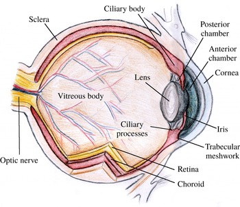
Sketch of a cross-section of the human eye.

In the present work we study the oscillatory and steady streaming flow in the anterior chamber (AC) of the eye generated during eye rotations. The bulk of the eye is filled with two main fluids: the vitreous and aqueous humours (see figure 1). The rheology of the vitreous humour is that of a gel with both viscous and elastic properties that are thought to contribute to its dynamics (David et al. Reference David, Smye, Dabbs and James1998; Meskauskas, Repetto & Siggers Reference Meskauskas, Repetto and Siggers2011, Reference Meskauskas, Repetto and Siggers2012), while the aqueous humour is well characterised as a Newtonian fluid with rheological properties similar to those of water. Aqueous humour is produced by the ciliary processes at a rate of approximately $3~\unicode[STIX]{x03BC}\text{l}~\text{min}^{-1}$ (Brubaker Reference Brubaker1991) per eye, from where it flows in the posterior chamber, enters the AC through the pupil and is eventually drained through the trabecular meshwork and out of the eye.

In spite of being slow, aqueous flow has important functions, since the balance between the rate of production and resistance to drainage determines the intraocular pressure. This is particularly relevant clinically, as an elevated intraocular pressure is correlated with the occurrence of open angle glaucoma (Sommer et al. Reference Sommer, Tielsch, Katz, Quigley, Gottsch, Javitt and Singh1991). The flow of aqueous humour is also important in the supply of nutrients to the avascular tissues of the lens and the cornea. Drugs placed on the surface of the eye are mainly drained into the AC, and their transport through the AC is strongly dependent on the flow of the aqueous humour (Urtti Reference Urtti2006). Furthermore, elevated shear stress on the cornea due to the flow of aqueous humour could lead to the detachment of endothelial cells from the cornea (Kaji et al. Reference Kaji, Oshika, Usui and Sakakibara2005).

Repetto et al. (Reference Repetto, Pralits, Siggers and Soleri2015) showed that, of the first three mechanisms listed in the previous paragraph, rotations of the eye produce the most intense flow in the AC, and thus contribute to the majority of the wall shear stress (WSS) on the cornea. Moreover, Abouali et al. (Reference Abouali, Modareszadeh, Ghaffarieh and Tu2012) showed that periodic rotations of the eye can produce a steady streaming flow that is intense enough to contribute to mixing at least as much as the thermally driven flow. When the eyes are closed during sleep, almost no thermal flow occurs in the AC, meaning that most of the mixing happens due to rapid eye movements (REM).

Analytical approaches based on lubrication theory have been extensively used to study the flow induced by aqueous secretion and the buoyancy-driven flow in the AC, after the seminal work by Canning et al. (Reference Canning, Greaney, Dewynne and Fitt2002). On the other hand, all previous investigations of the flow induced by eye rotations are based on fully numerical solutions of the Navier–Stokes equations. Although numerical simulations allow one to consider complex and very realistic geometries, they require large computational efforts, especially for time-dependent simulations, and make it difficult to obtain a clear picture of the dependency of the results on the controlling parameters. In this work we propose an analytical approach to study aqueous humour flow in the eye, which takes advantage of the small thickness of the AC, and use our results to investigate the parameter space more thoroughly than was previously possible.

Movements of the eye are routine and take a variety of different forms. Some rotations are close to periodic oscillations, and approximating them as a pure frequency oscillation has been a popular simplification in the literature, in both experimental works (Repetto, Stocchino & Cafferata Reference Repetto, Stocchino and Cafferata2005; Bonfiglio et al. Reference Bonfiglio, Repetto, Siggers and Stocchino2013, Reference Bonfiglio, Lagazzo, Repetto and Stocchino2015) and theoretical works (David et al. Reference David, Smye, Dabbs and James1998; Repetto, Siggers & Stocchino Reference Repetto, Siggers and Stocchino2010; Abouali et al. Reference Abouali, Modareszadeh, Ghaffarieh and Tu2012; Modarreszadeh et al. Reference Modarreszadeh, Abouali, Ghaffarieh and Ahmadi2014). In this work we also make use of this assumption.

As long as the shape of the AC does not change during an eye movement, the motion can be decomposed into a translational motion and an instantaneous rotational motion about an axis. In the case of pure translational motion, there would be no fluid motion relative to the domain, and the acceleration is balanced by a pressure gradient within the fluid. In this paper we simplify the problem to the case of rotational motion, and, furthermore, we assume the axis of rotations remains fixed. Thus, in principle, our work can be generalised to any motion of the eye, by adding a pressure gradient onto our solutions.

We model the AC as a thin domain sitting on the surface of a sphere that has either a constant height (in which case we can solve the problem analytically) or a more realistic shape (in which case we reduce the problem to a set of ordinary differential equations). We investigate both the primary oscillatory flow and the steady streaming, showing that both have a three-dimensional structure, the full details of which have not been highlighted by previous authors.

This paper is organised as follows. In § 2 the problem is formulated mathematically and simplified, and in § 3 the solution procedure is described. In § 4 we present the results, both in the constant height domain (§ 4.1) and for the more realistic geometry (§ 4.2). In § 5 we discuss the physiological and clinical relevance of the results.

2 Formulation of the problem

In this study we develop a model to find the motion of the aqueous humour during rotations of the eyeball. As discussed in the Introduction, the AC is relatively narrow in the anterior–posterior direction, and is delimited anteriorly by the cornea and posteriorly by the iris and lens (see figure 1 and the parameters given in table 1). In this model, we describe the iris and lens as a single continuous surface, thus neglecting the passage of the aqueous humour through the iris–lens channel, and hence also the turnover of the aqueous humour due to secretion and drainage. We justify this by comparing the flows found in the present model with those that would be expected due to aqueous humour turnover (e.g. Repetto et al. Reference Repetto, Pralits, Siggers and Soleri2015), and noting that the flows found in the present model are much larger.

2.1 Geometry of the domain

Figure 2.

(a) Sketch of the eye, showing the eyeball (large sphere) and the domain representing the AC attached to the sphere on the right. Sketch of the coordinate systems ${\mathcal{C}}$ and ${\mathcal{C}}^{\prime }$ . Cross-sections of the domains considered: (b) idealised constant-height domain; (c) more realistic representation of the AC geometry.

Table 1.

Geometrical characteristics of the domain and fluid properties.

To describe the eye rotations and the shape of the domain, it is convenient to introduce a set of Cartesian coordinates and two sets of spherical polar coordinates, which will be used interchangeably through the paper, and which are all illustrated in figure 2(a). The $z$ -axis of the Cartesian coordinates is the axis of rotation and the $x$ -axis points through the centre of the pupil. The set ${\mathcal{C}}=(r^{\ast },\unicode[STIX]{x1D703},\unicode[STIX]{x1D719})$ of spherical polar coordinates is convenient for describing the rotations, and has origin at the centre of the eye, $\unicode[STIX]{x1D703}=0$ along the axis of rotation and the centre of the pupil along the line $\unicode[STIX]{x1D703}=\unicode[STIX]{x03C0}/2$ , $\unicode[STIX]{x1D719}=0$ . Finally the set ${\mathcal{C}}^{\prime }=(r^{\ast },\unicode[STIX]{x1D703}^{\prime },\unicode[STIX]{x1D719}^{\prime })$ of spherical polar coordinates is convenient for describing the geometry of the AC, and is obtained by rotating ${\mathcal{C}}$ through $\unicode[STIX]{x03C0}/2$ about the $y$ -axis using right-handed rule of rotations. Thus it has the same origin, with the line $\unicode[STIX]{x1D703}^{\prime }=0$ through the centre of the pupil and the axis of rotation of the domain along $\unicode[STIX]{x1D703}^{\prime }=\unicode[STIX]{x03C0}/2$ , $\unicode[STIX]{x1D719}^{\prime }=0,\unicode[STIX]{x03C0}$ . The transformation from ${\mathcal{C}}$ to ${\mathcal{C}}^{\prime }$ can be performed using the following formulae (e.g. Meskauskas et al. Reference Meskauskas, Repetto and Siggers2011):

(2.1)

$$\begin{eqnarray}\left.\begin{array}{@{}c@{}}\cos \unicode[STIX]{x1D703}=-\text{sin}\unicode[STIX]{x1D703}^{\prime }\cos \unicode[STIX]{x1D719}^{\prime },\quad \cos \unicode[STIX]{x1D703}^{\prime }=\sin \unicode[STIX]{x1D703}\cos \unicode[STIX]{x1D719},\\ \tan \unicode[STIX]{x1D719}=\tan \unicode[STIX]{x1D703}^{\prime }\sin \unicode[STIX]{x1D719}^{\prime },\quad \tan \unicode[STIX]{x1D719}^{\prime }=-\text{tan}\unicode[STIX]{x1D703}\sin \unicode[STIX]{x1D719}.\end{array}\right\}\end{eqnarray}$$

To a good approximation, the AC is axisymmetric about the anterior–posterior axis ( $\unicode[STIX]{x1D703}^{\prime }=0$ ), and thus its geometry is independent of $\unicode[STIX]{x1D719}^{\prime }$ . We also assume for simplicity that its posterior surface (the iris and the lens) is a region of a spherical surface of radius $R$ centred on the centre of the eye (see figure 2 a). In particular we neglect the thickness of the inner boundary of the iris at the iris–lens channel, which is about 0.4 mm in reality. In addition, the assumption that the centre of the posterior spherical surface and the centre of the eye coincide is not necessary (in reality the radius of curvature of the lens is around 1 cm and that of the eye is 1.2 cm), but this allows us to find an analytical solution in the case of constant height. We denote the thickness of the AC as $h(\unicode[STIX]{x1D703}^{\prime })$ . We consider two cases: first, the case of uniform $h$ , in which we set $h$ equal to the maximum height $h=h_{max}$ , see figure 2(b), which allows us to find a completely analytical solution for the fluid flow; second, we consider a more realistic shape in which the domain is defined as $R\leqslant r^{\ast }\leqslant R+h(\unicode[STIX]{x1D703}^{\prime })$ for $0\leqslant \unicode[STIX]{x1D703}^{\prime }\leqslant \unicode[STIX]{x1D703}_{0}$ , where $h(\unicode[STIX]{x1D703}^{\prime })$ is a smooth monotonic decreasing function with $h(0)=h_{max}$ . In order to avoid numerical difficulties, we do not allow $h$ to reach zero at the outer boundary, and we arbitrarily set $h(\unicode[STIX]{x1D703}_{0})$ to the small value $h_{min}=h_{max}/50$ . We adopted the following expression for $h$ :

(2.2)

$$\begin{eqnarray}h=h_{max}\cos \unicode[STIX]{x1D703}^{\prime }+{\displaystyle \frac{h_{min}-h_{max}\cos \unicode[STIX]{x1D703}_{0}}{1-\cos \unicode[STIX]{x1D703}_{0}}}(1-\cos \unicode[STIX]{x1D703}^{\prime }),\end{eqnarray}$$

which is illustrated in figure 2(c). We typically use the parameter values given in table 1, except where otherwise stated, in which case the aspect ratio of the AC is $\unicode[STIX]{x1D716}=\overline{h}/R\approx 0.11$ , where $\overline{h}$ is the average height of the AC (volume of the AC divided by posterior surface area), defined below.

2.2 Eye rotations

In this work we consider harmonic rotational oscillations of the domain, with amplitude $\unicode[STIX]{x1D6FD}$ and angular frequency $\unicode[STIX]{x1D714}_{f}$ . Since we wish to apply our results to the flow in the AC during eye rotations, we adopt values representative of real eye movements and, in particular, of saccadic eye rotations and REM during sleep.

Saccadic rotations are performed to redirect the sight from one target to another, and they tend to be fast and of short duration. Becker (Reference Becker, Wurtz and Goldberg1989) proposed empirical relationships relating saccadic amplitude $A$ , duration $D$ , maximum angular velocity and acceleration time. We relate $\unicode[STIX]{x1D6FD}$ and $\unicode[STIX]{x1D714}_{f}$ using the fact that for saccadic rotations $D=D_{0}+dA$ , which is approximately valid in the range $5^{\circ }\lessapprox A\lessapprox 50^{\circ }$ , with $D$ measured in seconds and $A$ in degrees, $d\approx 0.0025$ s deg $^{-1}$ and $0.02\lessapprox D_{0}\lessapprox 0.03$ (Becker Reference Becker, Wurtz and Goldberg1989). To be able to model the eye rotations as saccadic movements, we assume that a period of rotation consists of two successive saccadic movements, each with amplitude $A$ and duration $D$ , and thus model the saccade as a harmonic rotation with amplitude $\unicode[STIX]{x1D6FD}=A/2$ and angular frequency $\unicode[STIX]{x1D714}_{f}=2\unicode[STIX]{x03C0}/(2D)=\unicode[STIX]{x03C0}/(D_{0}+2d\unicode[STIX]{x1D6FD})$ . Note that this approach to model periodic saccades differs from the one in Abouali et al. (Reference Abouali, Modareszadeh, Ghaffarieh and Tu2012), where those authors considered four saccadic movements per period instead of two. We non-dimensionalise this relationship by converting $\unicode[STIX]{x1D6FD}$ to radians and also working in terms of the Womersley number $\unicode[STIX]{x1D6FC}=\sqrt{\unicode[STIX]{x1D70C}\unicode[STIX]{x1D714}_{f}R^{2}/\unicode[STIX]{x1D707}}$ , where $\unicode[STIX]{x1D70C}$ is the fluid density and $\unicode[STIX]{x1D707}$ its shear viscosity (see table 1). This leads to the relationship shown by the curve in figure 3. REM is a normal feature of a particular phase of sleep, and consists of repeated side-to-side rotations that can have a wide range of amplitudes (Takahashi & Atsumi Reference Takahashi and Atsumi1997). For our model we adopt the same parameters as Modarreszadeh et al. (Reference Modarreszadeh, Abouali, Ghaffarieh and Ahmadi2014) and consider two cases: (i) ‘average REM’ with $\unicode[STIX]{x1D6FD}=6.27^{\circ }$ and $\unicode[STIX]{x1D714}_{f}=58.73\,^{\circ }\text{s}^{-1}$ , corresponding to the average of the experimental data of Takahashi & Atsumi (Reference Takahashi and Atsumi1997), and (ii) ‘maximum amplitude REM’ with $\unicode[STIX]{x1D6FD}=61.5^{\circ }$ and $\unicode[STIX]{x1D714}_{f}=491.98\,^{\circ }\text{s}^{-1}$ , which is the highest amplitude reported in the measurements, and these points are also reported in figure 3.

Figure 3.

Relationship between the Womersley number $\unicode[STIX]{x1D6FC}$ and the amplitude of rotations $\unicode[STIX]{x1D6FD}$ for saccadic eye rotations (curve), average REM (circle) and maximum amplitude REM (triangle) (Modarreszadeh et al. Reference Modarreszadeh, Abouali, Ghaffarieh and Ahmadi2014).

2.3 Derivation of the governing equations

In the following we work in a reference frame that rotates with the domain, and use superscript stars to denote dimensional variables that will be made dimensionless. Neglecting gravity, the continuity and Navier–Stokes equations become (e.g. Batchelor Reference Batchelor1967)

(2.3a )

$$\begin{eqnarray}\displaystyle & \displaystyle \unicode[STIX]{x1D735}^{\ast }\boldsymbol{\cdot }\boldsymbol{u}^{\ast }=0, & \displaystyle\end{eqnarray}$$

(2.3b )

$$\begin{eqnarray}\displaystyle & \displaystyle \unicode[STIX]{x1D70C}\left({\displaystyle \frac{\text{D}\boldsymbol{u}^{\ast }}{\text{D}t^{\ast }}}+\dot{\unicode[STIX]{x1D74E}}^{\ast }\times \boldsymbol{x}^{\ast }+2\unicode[STIX]{x1D74E}^{\ast }\times \boldsymbol{u}^{\ast }+(\unicode[STIX]{x1D74E}^{\ast }\boldsymbol{\cdot }\boldsymbol{x}^{\ast })\unicode[STIX]{x1D74E}^{\ast }-\unicode[STIX]{x1D714}^{\ast 2}\boldsymbol{x}^{\ast }\right)=-\unicode[STIX]{x1D735}^{\ast }p^{\ast }+\unicode[STIX]{x1D707}\unicode[STIX]{x1D6FB}^{2}\boldsymbol{u}^{\ast },\qquad & \displaystyle\end{eqnarray}$$

where

$\boldsymbol{u}^{\ast }$ is fluid velocity relative to the reference frame,

$p^{\ast }$ is the departure of the pressure from the hydrostatic profile (thus we omit the gravitational acceleration),

$\unicode[STIX]{x1D74E}^{\ast }$ is the prescribed angular velocity of the domain (and

$\unicode[STIX]{x1D714}^{\ast }=|\unicode[STIX]{x1D74E}^{\ast }|$ ),

$\boldsymbol{x}^{\ast }$ is the position vector,

$\unicode[STIX]{x1D735}^{\ast }$ is spatial gradient and

$\text{D}\boldsymbol{u}^{\ast }/\text{D}t^{\ast }$ denotes a dimensional material derivative. Recalling the utilised coordinate system

${\mathcal{C}}=(r^{\ast },\unicode[STIX]{x1D703},\unicode[STIX]{x1D719})$ , we consider sinusoidal rotations with prescribed angular displacement

$\unicode[STIX]{x1D6FD}\sin \unicode[STIX]{x1D714}_{f}t^{\ast }$ about the axis

$\unicode[STIX]{x1D703}=0$ (

$z=0$ ), giving the angular velocity

$\unicode[STIX]{x1D74E}^{\ast }=\unicode[STIX]{x1D714}^{\ast }(\cos \unicode[STIX]{x1D703},-\text{sin}\unicode[STIX]{x1D703},0)$ with magnitude

$\unicode[STIX]{x1D714}^{\ast }=\unicode[STIX]{x1D6FD}\unicode[STIX]{x1D714}_{f}\cos \unicode[STIX]{x1D714}_{f}t^{\ast }$ .

A characteristic depth of the AC may be obtained by calculating the volume of the AC divided by inner surface area, which, assuming $h\ll R$ , is approximately $\overline{h}=\int _{0}^{\unicode[STIX]{x1D703}_{0}}h(\unicode[STIX]{x1D703}^{\prime })\sin (\unicode[STIX]{x1D703}^{\prime })\,\text{d}\unicode[STIX]{x1D703}^{\prime }/(1-\cos (\unicode[STIX]{x1D703}_{0}))$ . Dividing by the length of the chamber gives the aspect ratio of the AC $\unicode[STIX]{x1D716}=\overline{h}/(2R\unicode[STIX]{x1D703}_{0})$ .

We introduce the following scales for non-dimensionalisation:

(2.4)

$$\begin{eqnarray}\left.\begin{array}{@{}c@{}}r^{\ast }=R+\overline{h}r,\quad t^{\ast }={\displaystyle \frac{t}{\unicode[STIX]{x1D714}_{f}}},\quad u_{\unicode[STIX]{x1D719}}^{\ast }=Uu_{\unicode[STIX]{x1D719}},\quad u_{\unicode[STIX]{x1D703}}^{\ast }=Uu_{\unicode[STIX]{x1D703}},\quad u_{r}^{\ast }=\unicode[STIX]{x1D716}Uu_{r},\\ p^{\ast }=P_{0}p,\quad \unicode[STIX]{x1D714}^{\ast }=\unicode[STIX]{x1D6FD}\unicode[STIX]{x1D714}_{f}\unicode[STIX]{x1D714}.\end{array}\right\}\end{eqnarray}$$

We choose $U=\overline{h}\unicode[STIX]{x1D6FD}\unicode[STIX]{x1D714}_{f}$ as the velocity scale and $P_{0}=R^{2}\unicode[STIX]{x1D714}_{f}^{2}\unicode[STIX]{x1D6FD}\unicode[STIX]{x1D70C}$ as the pressure scale (chosen so that the pressure gradient in the $\unicode[STIX]{x1D719}$ direction balances the angular acceleration term), and let $\unicode[STIX]{x1D716}=\overline{h}/R$ be the approximate aspect ratio of the domain.

With the above scales, the dimensionless continuity and Navier–Stokes equations (2.3) read

(2.5a )

$$\begin{eqnarray}\displaystyle & & \displaystyle {\displaystyle \frac{\unicode[STIX]{x2202}u_{r}}{\unicode[STIX]{x2202}r}}+{\displaystyle \frac{1}{\sin \unicode[STIX]{x1D703}}}{\displaystyle \frac{\unicode[STIX]{x2202}}{\unicode[STIX]{x2202}\unicode[STIX]{x1D703}}}\left(u_{\unicode[STIX]{x1D703}}\sin \unicode[STIX]{x1D703}\right)+{\displaystyle \frac{1}{\sin \unicode[STIX]{x1D703}}}{\displaystyle \frac{\unicode[STIX]{x2202}u_{\unicode[STIX]{x1D719}}}{\unicode[STIX]{x2202}\unicode[STIX]{x1D719}}}+\unicode[STIX]{x1D716}\left(r{\displaystyle \frac{\unicode[STIX]{x2202}u_{r}}{\unicode[STIX]{x2202}r}}+2u_{r}\right)=0,\end{eqnarray}$$

(2.5b )

$$\begin{eqnarray}\displaystyle & & \displaystyle \unicode[STIX]{x1D716}^{3}{\displaystyle \frac{\unicode[STIX]{x2202}u_{r}}{\unicode[STIX]{x2202}t}}+\unicode[STIX]{x1D716}^{4}\unicode[STIX]{x1D6FD}\boldsymbol{u}\boldsymbol{\cdot }\unicode[STIX]{x1D735}u_{r}-\unicode[STIX]{x1D716}^{3}\unicode[STIX]{x1D6FD}{\displaystyle \frac{u_{\unicode[STIX]{x1D719}}^{2}+u_{\unicode[STIX]{x1D703}}^{2}}{1+\unicode[STIX]{x1D716}r}}-2\unicode[STIX]{x1D6FD}\unicode[STIX]{x1D716}^{2}\unicode[STIX]{x1D714}u_{\unicode[STIX]{x1D719}}\sin \unicode[STIX]{x1D703}-\unicode[STIX]{x1D716}\unicode[STIX]{x1D6FD}\unicode[STIX]{x1D714}^{2}(1+\unicode[STIX]{x1D716}r)\sin ^{2}\unicode[STIX]{x1D703}\nonumber\\ \displaystyle & & \displaystyle \quad =-{\displaystyle \frac{\unicode[STIX]{x2202}p}{\unicode[STIX]{x2202}r}}+{\displaystyle \frac{\unicode[STIX]{x1D716}}{\unicode[STIX]{x1D6FC}^{2}}}\left(\unicode[STIX]{x1D6FB}^{2}u_{r}-\unicode[STIX]{x1D716}^{2}{\displaystyle \frac{2u_{r}}{(1+\unicode[STIX]{x1D716}r)^{2}}}-{\displaystyle \frac{2\unicode[STIX]{x1D716}}{(1+\unicode[STIX]{x1D716}r)^{2}\sin \unicode[STIX]{x1D703}}}\left({\displaystyle \frac{\unicode[STIX]{x2202}(u_{\unicode[STIX]{x1D703}}\sin \unicode[STIX]{x1D703})}{\unicode[STIX]{x2202}\unicode[STIX]{x1D703}}}+\unicode[STIX]{x1D716}{\displaystyle \frac{\unicode[STIX]{x2202}u_{\unicode[STIX]{x1D719}}}{\unicode[STIX]{x2202}\unicode[STIX]{x1D719}}}\right)\!\right),\nonumber\\ \displaystyle & & \displaystyle\end{eqnarray}$$

(2.5c )

$$\begin{eqnarray}\displaystyle & & \displaystyle \unicode[STIX]{x1D716}{\displaystyle \frac{\unicode[STIX]{x2202}u_{\unicode[STIX]{x1D703}}}{\unicode[STIX]{x2202}t}}+\unicode[STIX]{x1D716}^{2}\unicode[STIX]{x1D6FD}\boldsymbol{u}\boldsymbol{\cdot }\unicode[STIX]{x1D735}u_{\unicode[STIX]{x1D703}}+\unicode[STIX]{x1D716}^{3}\unicode[STIX]{x1D6FD}{\displaystyle \frac{u_{r}u_{\unicode[STIX]{x1D703}}}{1+\unicode[STIX]{x1D716}r}}-\unicode[STIX]{x1D716}^{2}\unicode[STIX]{x1D6FD}{\displaystyle \frac{u_{\unicode[STIX]{x1D719}}^{2}\cot \unicode[STIX]{x1D703}}{1+\unicode[STIX]{x1D716}r}}\nonumber\\ \displaystyle & & \displaystyle \qquad -\,2\unicode[STIX]{x1D716}\unicode[STIX]{x1D6FD}\unicode[STIX]{x1D714}\cos \unicode[STIX]{x1D703}u_{\unicode[STIX]{x1D719}}-\unicode[STIX]{x1D6FD}\unicode[STIX]{x1D714}^{2}(1+\unicode[STIX]{x1D716}r)\cos \unicode[STIX]{x1D703}\sin \unicode[STIX]{x1D703}\nonumber\\ \displaystyle & & \displaystyle \quad =-{\displaystyle \frac{1}{1+\unicode[STIX]{x1D716}r}}{\displaystyle \frac{\unicode[STIX]{x2202}p}{\unicode[STIX]{x2202}\unicode[STIX]{x1D703}}}+{\displaystyle \frac{1}{\unicode[STIX]{x1D716}\unicode[STIX]{x1D6FC}^{2}}}\left(\unicode[STIX]{x1D6FB}^{2}u_{\unicode[STIX]{x1D703}}+{\displaystyle \frac{2\unicode[STIX]{x1D716}^{3}}{(1+\unicode[STIX]{x1D716}r)^{2}}}{\displaystyle \frac{\unicode[STIX]{x2202}u_{r}}{\unicode[STIX]{x2202}\unicode[STIX]{x1D703}}}-{\displaystyle \frac{\unicode[STIX]{x1D716}^{2}}{r^{2}\sin ^{2}\unicode[STIX]{x1D703}}}\left(u_{\unicode[STIX]{x1D703}}+2\cos \unicode[STIX]{x1D703}{\displaystyle \frac{\unicode[STIX]{x2202}u_{\unicode[STIX]{x1D719}}}{\unicode[STIX]{x2202}\unicode[STIX]{x1D719}}}\right)\!\right),\nonumber\\ \displaystyle & & \displaystyle\end{eqnarray}$$

(2.5d )

$$\begin{eqnarray}\displaystyle & & \displaystyle \unicode[STIX]{x1D716}{\displaystyle \frac{\unicode[STIX]{x2202}u_{\unicode[STIX]{x1D719}}}{\unicode[STIX]{x2202}t}}+\unicode[STIX]{x1D716}^{2}\unicode[STIX]{x1D6FD}\boldsymbol{u}\boldsymbol{\cdot }\unicode[STIX]{x1D735}u_{\unicode[STIX]{x1D719}}+\unicode[STIX]{x1D716}^{3}\unicode[STIX]{x1D6FD}{\displaystyle \frac{u_{\unicode[STIX]{x1D719}}u_{r}}{r}}+\unicode[STIX]{x1D716}^{2}\unicode[STIX]{x1D6FD}{\displaystyle \frac{u_{\unicode[STIX]{x1D703}}u_{\unicode[STIX]{x1D719}}\cot \unicode[STIX]{x1D703}}{r}}+(1+\unicode[STIX]{x1D716}r)\dot{\unicode[STIX]{x1D714}}\sin \unicode[STIX]{x1D703}\nonumber\\ \displaystyle & & \displaystyle +\,2\unicode[STIX]{x1D716}\unicode[STIX]{x1D6FD}\unicode[STIX]{x1D714}(u_{\unicode[STIX]{x1D703}}\cos \unicode[STIX]{x1D703}+\unicode[STIX]{x1D716}u_{r}\sin \unicode[STIX]{x1D703})=-{\displaystyle \frac{1}{(1+\unicode[STIX]{x1D716}r)\sin \unicode[STIX]{x1D703}}}{\displaystyle \frac{\unicode[STIX]{x2202}p}{\unicode[STIX]{x2202}\unicode[STIX]{x1D719}}}\nonumber\\ \displaystyle & & \displaystyle +\,{\displaystyle \frac{1}{\unicode[STIX]{x1D716}\unicode[STIX]{x1D6FC}^{2}}}\left(\unicode[STIX]{x1D6FB}^{2}u_{\unicode[STIX]{x1D719}}+{\displaystyle \frac{2\unicode[STIX]{x1D716}^{2}}{(1+\unicode[STIX]{x1D716}r)^{2}\sin \unicode[STIX]{x1D703}}}\left({\displaystyle \frac{\unicode[STIX]{x2202}u_{r}}{\unicode[STIX]{x2202}\unicode[STIX]{x1D719}}}+\cot \unicode[STIX]{x1D703}{\displaystyle \frac{\unicode[STIX]{x2202}u_{\unicode[STIX]{x1D719}}}{\unicode[STIX]{x2202}\unicode[STIX]{x1D719}}}\right)-\unicode[STIX]{x1D716}^{3}{\displaystyle \frac{u_{\unicode[STIX]{x1D719}}}{(1+\unicode[STIX]{x1D716}r)^{2}\sin ^{2}\unicode[STIX]{x1D703}}}\right),\end{eqnarray}$$

with

$\unicode[STIX]{x1D714}=\cos t$ and

$\dot{\unicode[STIX]{x1D714}}=-\text{sin}t$ , and

(2.6)

$$\begin{eqnarray}\displaystyle \unicode[STIX]{x1D6FB}^{2}f & = & \displaystyle {\displaystyle \frac{\unicode[STIX]{x2202}^{2}f}{\unicode[STIX]{x2202}r^{2}}}+{\displaystyle \frac{2\unicode[STIX]{x1D716}}{1+\unicode[STIX]{x1D716}r}}{\displaystyle \frac{\unicode[STIX]{x2202}f}{\unicode[STIX]{x2202}r}}+{\displaystyle \frac{\unicode[STIX]{x1D716}^{2}}{(1+\unicode[STIX]{x1D716}r)^{2}\sin \unicode[STIX]{x1D703}}}{\displaystyle \frac{\unicode[STIX]{x2202}}{\unicode[STIX]{x2202}\unicode[STIX]{x1D703}}}\left(\sin \unicode[STIX]{x1D703}{\displaystyle \frac{\unicode[STIX]{x2202}f}{\unicode[STIX]{x2202}\unicode[STIX]{x1D703}}}\right)+{\displaystyle \frac{\unicode[STIX]{x1D716}^{2}}{\sin ^{2}\unicode[STIX]{x1D703}(1+\unicode[STIX]{x1D716}r)^{2}}}{\displaystyle \frac{\unicode[STIX]{x2202}^{2}f}{\unicode[STIX]{x2202}\unicode[STIX]{x1D719}^{2}}}\nonumber\\ \displaystyle & & \displaystyle ={\displaystyle \frac{\unicode[STIX]{x2202}^{2}f}{\unicode[STIX]{x2202}r^{2}}}+2\unicode[STIX]{x1D716}{\displaystyle \frac{\unicode[STIX]{x2202}f}{\unicode[STIX]{x2202}r}}+O(\unicode[STIX]{x1D716}^{2}),\end{eqnarray}$$

for any function $f$ .

Using the geometrical values from table 1, we estimate

(2.7a,b )

$$\begin{eqnarray}\displaystyle & \unicode[STIX]{x1D716}\approx 0.11,\quad \unicode[STIX]{x1D716}^{2}\approx 0.012, & \displaystyle\end{eqnarray}$$

and in table 2 we report the remaining dimensionless parameters appearing in the governing equations (2.5) in four cases (taken from the data in figure 3): small and large saccadic rotations (amplitude $5^{\circ }$ and $50^{\circ }$ , respectively), average REM and maximum amplitude REM.

Table 2.

Typical values of the dimensionless parameters, with $\unicode[STIX]{x1D716}\approx 0.11$ in all cases.

In the remainder of this work we drop from (2.5) any terms of orders $\unicode[STIX]{x1D716}^{2}$ , $\unicode[STIX]{x1D716}\unicode[STIX]{x1D6FD}$ and $1/\unicode[STIX]{x1D6FC}^{2}$ , which can be seen to be small from table 2, as well as smaller terms. This leaves terms of order 1, $\unicode[STIX]{x1D6FD}$ , $\unicode[STIX]{x1D716}$ and $1/(\unicode[STIX]{x1D716}\unicode[STIX]{x1D6FC}^{2})$ . Despite the fact that $1/(\unicode[STIX]{x1D716}\unicode[STIX]{x1D6FC}^{2})$ is typically smaller than both $\unicode[STIX]{x1D716}^{2}$ and $\unicode[STIX]{x1D716}\unicode[STIX]{x1D6FD}$ we choose to keep terms with this coefficient, as they are not negligible within the boundary layer. The same approach was used by Blondeaux & Vittori (Reference Blondeaux and Vittori1994) for a different problem, who showed that it leads to the same results as formal boundary layer analysis. Note also that for maximum amplitude REM, terms of order $\unicode[STIX]{x1D716}\unicode[STIX]{x1D6FD}$ are comparable to those of order $\unicode[STIX]{x1D716}$ , implying that the model might not be very accurate in this case.

With the above simplifications we obtain the following system:

(2.8a )

$$\begin{eqnarray}\displaystyle & \displaystyle {\displaystyle \frac{\unicode[STIX]{x2202}p}{\unicode[STIX]{x2202}r}}=0, & \displaystyle\end{eqnarray}$$

(2.8b )

$$\begin{eqnarray}\displaystyle & \displaystyle \unicode[STIX]{x1D716}{\displaystyle \frac{\unicode[STIX]{x2202}u_{\unicode[STIX]{x1D703}}}{\unicode[STIX]{x2202}t}}-\unicode[STIX]{x1D6FD}\unicode[STIX]{x1D714}^{2}\cos \unicode[STIX]{x1D703}\sin \unicode[STIX]{x1D703}=-(1-\unicode[STIX]{x1D716}r){\displaystyle \frac{\unicode[STIX]{x2202}p}{\unicode[STIX]{x2202}\unicode[STIX]{x1D703}}}+{\displaystyle \frac{1}{\unicode[STIX]{x1D716}\unicode[STIX]{x1D6FC}^{2}}}{\displaystyle \frac{\unicode[STIX]{x2202}^{2}u_{\unicode[STIX]{x1D703}}}{\unicode[STIX]{x2202}r^{2}}}, & \displaystyle\end{eqnarray}$$

(2.8c )

$$\begin{eqnarray}\displaystyle & \displaystyle \unicode[STIX]{x1D716}{\displaystyle \frac{\unicode[STIX]{x2202}u_{\unicode[STIX]{x1D719}}}{\unicode[STIX]{x2202}t}}+(1+\unicode[STIX]{x1D716}r)\dot{\unicode[STIX]{x1D714}}\sin \unicode[STIX]{x1D703}=-{\displaystyle \frac{1-\unicode[STIX]{x1D716}r}{\sin \unicode[STIX]{x1D703}}}{\displaystyle \frac{\unicode[STIX]{x2202}p}{\unicode[STIX]{x2202}\unicode[STIX]{x1D719}}}+{\displaystyle \frac{1}{\unicode[STIX]{x1D716}\unicode[STIX]{x1D6FC}^{2}}}{\displaystyle \frac{\unicode[STIX]{x2202}^{2}u_{\unicode[STIX]{x1D719}}}{\unicode[STIX]{x2202}r^{2}}}, & \displaystyle\end{eqnarray}$$

coupled to the continuity equation (2.5a ), which remains in full. Equations (2.8) should be solved subject to no-penetration and no-slip boundary conditions at

$r=0$ and

$r=h(\unicode[STIX]{x1D703},\unicode[STIX]{x1D719})/\bar{h}$ and zero flux at

$\unicode[STIX]{x1D703}^{\prime }=\unicode[STIX]{x1D703}_{0}$ . We note that the latter does not imply no-slip condition at the boundary

$\unicode[STIX]{x1D703}^{\prime }=\unicode[STIX]{x1D703}_{0}$ and is a consequence of the application of lubrication theory. Therefore, the solution close to

$\unicode[STIX]{x1D703}^{\prime }=\unicode[STIX]{x1D703}_{0}$ is not accurate. We also require the solution to be regular at

$\unicode[STIX]{x1D703}^{\prime }=0$ .

3 Solution

3.1 Decomposition of the solution

As is usual in lubrication theory, (2.8a ) shows that the pressure does not depend on the $r$ -coordinate. The motion is forced by the term proportional to $\unicode[STIX]{x1D714}^{2}$ in (2.8b ) and that proportional to $\dot{\unicode[STIX]{x1D714}}$ in (2.8c ). Recalling that $\unicode[STIX]{x1D714}=\cos t=\text{e}^{\text{i}t}/2+\text{c.c.}$ , where c.c. denotes the complex conjugate, we note that three frequencies are effectively forced, 0, 1 and 2, corresponding to the terms proportional to $\text{e}^{0\text{i}t}$ , $\text{e}^{\text{i}t}$ and $\text{e}^{2\text{i}t}$ . In other words, harmonic oscillations of the domain with dimensionless frequency 1 force a steady streaming component, a flow with the same frequency as the forcing and also flow at twice that frequency. Thus, we seek a solution for the velocity and the pressure in the form

(3.1)

$$\begin{eqnarray}\displaystyle & \displaystyle \boldsymbol{u}(\boldsymbol{x},t)=\boldsymbol{u}^{(0)}(\boldsymbol{x})+\boldsymbol{u}^{(1)}(\boldsymbol{x})\text{e}^{\text{i}t}+\boldsymbol{u}^{(2)}(\boldsymbol{x})\text{e}^{2\text{i}t}+\text{c.c.}, & \displaystyle\end{eqnarray}$$

(3.2)

$$\begin{eqnarray}\displaystyle & \displaystyle p(\boldsymbol{x},t)=p^{(0)}(\boldsymbol{x})+p^{(1)}(\boldsymbol{x})\text{e}^{\text{i}t}+p^{(2)}(\boldsymbol{x})\text{e}^{2\text{i}t}+\text{c.c.} & \displaystyle\end{eqnarray}$$

Substituting into (2.8a-c ) we obtain the following set of equations for $k=0,1,2$ , respectively:

(3.3a )

$$\begin{eqnarray}\displaystyle & \displaystyle {\displaystyle \frac{\unicode[STIX]{x2202}p^{(k)}}{\unicode[STIX]{x2202}r}}=0, & \displaystyle\end{eqnarray}$$

(3.3b )

$$\begin{eqnarray}\displaystyle & \displaystyle \text{i}k\unicode[STIX]{x1D716}u_{\unicode[STIX]{x1D703}}^{(k)}-{\displaystyle \frac{1}{\unicode[STIX]{x1D716}\unicode[STIX]{x1D6FC}^{2}}}{\displaystyle \frac{\unicode[STIX]{x2202}^{2}u_{\unicode[STIX]{x1D703}}^{(k)}}{\unicode[STIX]{x2202}r^{2}}}=-(1-\unicode[STIX]{x1D716}r){\displaystyle \frac{\unicode[STIX]{x2202}p^{(k)}}{\unicode[STIX]{x2202}\unicode[STIX]{x1D703}}}+\unicode[STIX]{x1D6E9}^{(k)}, & \displaystyle\end{eqnarray}$$

(3.3c )

$$\begin{eqnarray}\displaystyle & \displaystyle \text{i}k\unicode[STIX]{x1D716}u_{\unicode[STIX]{x1D719}}^{(k)}-{\displaystyle \frac{1}{\unicode[STIX]{x1D716}\unicode[STIX]{x1D6FC}^{2}}}{\displaystyle \frac{\unicode[STIX]{x2202}^{2}u_{\unicode[STIX]{x1D719}}^{(k)}}{\unicode[STIX]{x2202}r^{2}}}=-{\displaystyle \frac{1-\unicode[STIX]{x1D716}r}{\sin \unicode[STIX]{x1D703}}}{\displaystyle \frac{\unicode[STIX]{x2202}p^{(k)}}{\unicode[STIX]{x2202}\unicode[STIX]{x1D719}}}+\unicode[STIX]{x1D6F7}^{(k)}, & \displaystyle\end{eqnarray}$$

where

$\unicode[STIX]{x1D6E9}^{(0)}=\unicode[STIX]{x1D6E9}^{(2)}=(\unicode[STIX]{x1D6FD}/8)\sin (2\unicode[STIX]{x1D703})$ ,

$\unicode[STIX]{x1D6F7}^{(1)}=-(\text{i}/2)(1+\unicode[STIX]{x1D716}r)\sin \unicode[STIX]{x1D703}$ and

$\unicode[STIX]{x1D6E9}^{(1)}=\unicode[STIX]{x1D6F7}^{(0)}=\unicode[STIX]{x1D6F7}^{(2)}=0$ . Equations (3.3) are coupled with the continuity equation for each harmonic.

3.2 Derivation of the equation for the pressure

Following the standard approach in lubrication theory, we solve (3.3b ) and (3.3c ) to find the $r$ -dependence of $u_{\unicode[STIX]{x1D703}}^{(k)}$ and $u_{\unicode[STIX]{x1D719}}^{(k)}$ , respectively, which, when combined with the no-slip boundary conditions, gives

(3.4)

$$\begin{eqnarray}\boldsymbol{u}_{\mathit{h}}^{(k)}=A_{k}(r,h)\unicode[STIX]{x1D735}_{\mathit{h}}p^{(k)}+B_{k}(r,h)\boldsymbol{v}_{k},\end{eqnarray}$$

for $k=0,1,2$ , where $\boldsymbol{v}_{0}=\boldsymbol{v}_{2}=\sin 2\unicode[STIX]{x1D703}\boldsymbol{e}_{\unicode[STIX]{x1D703}}$ , $\boldsymbol{v}_{1}=\sin \unicode[STIX]{x1D703}\boldsymbol{e}_{\unicode[STIX]{x1D719}}$ and the functions $A_{k}$ and $B_{k}$ are reported in appendix A. The unit vectors $\boldsymbol{e}_{\unicode[STIX]{x1D703}}$ and $\boldsymbol{e}_{\unicode[STIX]{x1D719}}$ point in the directions of increasing $\unicode[STIX]{x1D703}$ and $\unicode[STIX]{x1D719}$ , respectively, and a subscript $h$ on a vector indicates that the projection of the vector on the $\unicode[STIX]{x1D703}$ and $\unicode[STIX]{x1D719}$ directions is taken.

It is convenient from now on to work in the coordinate system ${\mathcal{C}}^{\prime }$ defined in § 2.1, so that we can make use of the fact that the domain is axisymmetric with respect to $\unicode[STIX]{x1D703}^{\prime }=0$ (see figure 2 a). In this coordinate system (3.4) takes the form

(3.5)

$$\begin{eqnarray}\boldsymbol{u}_{\mathit{h}}^{(k)}=A_{k}(r,h)\unicode[STIX]{x1D735}_{\mathit{h}}^{\prime }p^{(k)}+B_{k}(r,h)\boldsymbol{v}_{k}^{\prime },\end{eqnarray}$$

where $\boldsymbol{v}_{0}^{\prime }=\boldsymbol{v}_{2}^{\prime }=-\text{sin}2\unicode[STIX]{x1D703}^{\prime }\cos ^{2}\unicode[STIX]{x1D719}^{\prime }\boldsymbol{e}_{\unicode[STIX]{x1D703}^{\prime }}+\sin 2\unicode[STIX]{x1D719}^{\prime }\sin \unicode[STIX]{x1D703}^{\prime }\boldsymbol{e}_{\unicode[STIX]{x1D719}^{\prime }}$ , $\boldsymbol{v}_{1}^{\prime }=\sin \unicode[STIX]{x1D719}^{\prime }\boldsymbol{e}_{\unicode[STIX]{x1D703}^{\prime }}+\cos \unicode[STIX]{x1D703}^{\prime }\cos \unicode[STIX]{x1D719}^{\prime }\boldsymbol{e}_{\unicode[STIX]{x1D719}^{\prime }}$ and $\unicode[STIX]{x1D735}^{\prime }$ are vectors $\boldsymbol{v}_{k},~k=0,1,2$ and $\unicode[STIX]{x1D735}$ expressed in ${\mathcal{C}}^{\prime }$ coordinate system. Substituting (3.5) into the continuity equation (2.5a ) and integrating it over $r$ , we obtain a partial differential equation for $p^{(k)}$ for $k=0,1,2$ :

(3.6)

$$\begin{eqnarray}{\mathcal{A}}(\unicode[STIX]{x1D6FE}_{k})p^{(k)}+{\mathcal{B}}_{k}(\unicode[STIX]{x1D6FF}_{k})=0,\end{eqnarray}$$

where

(3.7a,b )

$$\begin{eqnarray}\unicode[STIX]{x1D6FE}_{k}(h)=\int _{0}^{h}(1+\unicode[STIX]{x1D716}r)A_{k}(r,h)\,\text{d}r,\quad \unicode[STIX]{x1D6FF}_{k}(h)=\int _{0}^{h}(1+\unicode[STIX]{x1D716}r)B_{k}(r,h)\,\text{d}r\end{eqnarray}$$

(explicit expressions for $\unicode[STIX]{x1D6FE}_{k}$ and $\unicode[STIX]{x1D6FF}_{k}$ appear in appendix A) and ${\mathcal{A}}(\unicode[STIX]{x1D6FE}_{k})$ is a linear differential operator given by

(3.8)

$$\begin{eqnarray}{\mathcal{A}}(\unicode[STIX]{x1D6FE}_{k})={\displaystyle \frac{1}{\sin \unicode[STIX]{x1D703}^{\prime }}}\left({\displaystyle \frac{\unicode[STIX]{x2202}}{\unicode[STIX]{x2202}\unicode[STIX]{x1D703}^{\prime }}}\left(\sin \unicode[STIX]{x1D703}^{\prime }\unicode[STIX]{x1D6FE}_{k}{\displaystyle \frac{\unicode[STIX]{x2202}}{\unicode[STIX]{x2202}\unicode[STIX]{x1D703}^{\prime }}}\right)+{\displaystyle \frac{\unicode[STIX]{x1D6FE}_{k}}{\sin \unicode[STIX]{x1D703}^{\prime }}}{\displaystyle \frac{\unicode[STIX]{x2202}^{2}}{\unicode[STIX]{x2202}{\unicode[STIX]{x1D719}^{\prime }}^{2}}}\right),\end{eqnarray}$$

with

(3.9a )

$$\begin{eqnarray}\displaystyle & \displaystyle {\mathcal{B}}_{0}(\unicode[STIX]{x1D6FF}_{0})=2\left(3\sin ^{2}\unicode[STIX]{x1D703}^{\prime }\cos ^{2}\unicode[STIX]{x1D719}^{\prime }-1\right)\unicode[STIX]{x1D6FF}_{0}(h)-2\cos ^{2}\unicode[STIX]{x1D719}^{\prime }\sin \unicode[STIX]{x1D703}^{\prime }\cos \unicode[STIX]{x1D703}^{\prime }{\displaystyle \frac{\text{d}\unicode[STIX]{x1D6FF}_{0}(h)}{\text{d}\unicode[STIX]{x1D703}^{\prime }}}, & \displaystyle\end{eqnarray}$$

(3.9b )

$$\begin{eqnarray}\displaystyle & \displaystyle {\mathcal{B}}_{1}(\unicode[STIX]{x1D6FF}_{1})=\sin \unicode[STIX]{x1D719}^{\prime }{\displaystyle \frac{\unicode[STIX]{x2202}\unicode[STIX]{x1D6FF}_{1}}{\unicode[STIX]{x2202}\unicode[STIX]{x1D703}^{\prime }}}, & \displaystyle\end{eqnarray}$$

(3.9c )

$$\begin{eqnarray}\displaystyle & \displaystyle {\mathcal{B}}_{2}(\unicode[STIX]{x1D6FF}_{2})={\mathcal{B}}_{0}(\unicode[STIX]{x1D6FF}_{2}). & \displaystyle\end{eqnarray}$$

The

$r$ -integrated velocity, or flux per unit length, reads

(3.10)

$$\begin{eqnarray}\displaystyle \boldsymbol{q}_{\mathit{h}}^{(k)}=\int _{0}^{h}(1+\unicode[STIX]{x1D716}r)\boldsymbol{u}_{\mathit{h}}^{(k)}\,\text{d}r=\unicode[STIX]{x1D6FE}_{k}\unicode[STIX]{x1D735}_{\mathit{h}}^{\prime }p^{(k)}+\unicode[STIX]{x1D6FF}_{k}\boldsymbol{v}_{k}^{\prime }, & & \displaystyle\end{eqnarray}$$

where $\unicode[STIX]{x1D735}_{\mathit{h}}^{\prime }$ is computed on the spherical surface $r=1$ .

The no-flux condition at the boundary $\unicode[STIX]{x1D703}^{\prime }=\unicode[STIX]{x1D703}_{0}$ can then be written as

(3.11)

$$\begin{eqnarray}\boldsymbol{q}_{\mathit{h}}^{(k)}\boldsymbol{\cdot }\boldsymbol{e}_{\unicode[STIX]{x1D703}^{\prime }}=0\quad \Rightarrow \quad \unicode[STIX]{x1D6FE}_{k}{\displaystyle \frac{\unicode[STIX]{x2202}p^{(k)}}{\unicode[STIX]{x2202}\unicode[STIX]{x1D703}^{\prime }}}+\unicode[STIX]{x1D6FF}_{k}\boldsymbol{v}_{k}^{\prime }\boldsymbol{\cdot }\boldsymbol{e}_{\unicode[STIX]{x1D703}^{\prime }}=0,\end{eqnarray}$$

and we also require the solution $p^{(k)}$ to be regular (in this case, continuous and with continuous derivative) at $\unicode[STIX]{x1D703}^{\prime }=0$ . Note that each $p^{(k)}$ is uniquely defined up to the addition of an arbitrary constant. Thus, in what follows, without loss of generality, we assume that $p^{(k)}=0$ at $\unicode[STIX]{x1D703}^{\prime }=0$ .

In the following subsections, we simplify the problem for each harmonic $k=0,1,2$ by separating the $\unicode[STIX]{x1D703}^{\prime }$ - and $\unicode[STIX]{x1D719}^{\prime }$ -dependence, and we derive an analytical solution for each in the case of constant $h$ .

3.3 Separation of variables and solution for the case of constant $h$

3.3.1 Dominant frequency component ( $k=1$ )

For the case $k=1$ we note the $\unicode[STIX]{x1D719}^{\prime }$ -dependence in (3.6) and (3.11) and seek a solution of the form

(3.12)

$$\begin{eqnarray}\displaystyle p^{(1)}(\unicode[STIX]{x1D703}^{\prime },\unicode[STIX]{x1D719}^{\prime })=g(\unicode[STIX]{x1D703}^{\prime })\sin \unicode[STIX]{x1D719}^{\prime }. & & \displaystyle\end{eqnarray}$$

This leads to

(3.13a )

$$\begin{eqnarray}\displaystyle {\displaystyle \frac{1}{\sin \unicode[STIX]{x1D703}^{\prime }}}{\displaystyle \frac{\text{d}}{\text{d}\unicode[STIX]{x1D703}^{\prime }}}\left(\sin \unicode[STIX]{x1D703}^{\prime }\unicode[STIX]{x1D6FE}_{1}{\displaystyle \frac{\text{d}g}{\text{d}\unicode[STIX]{x1D703}^{\prime }}}\right)-{\displaystyle \frac{\unicode[STIX]{x1D6FE}_{1}}{\sin ^{2}\unicode[STIX]{x1D703}^{\prime }}}g+{\displaystyle \frac{\text{d}\unicode[STIX]{x1D6FF}_{1}}{\text{d}\unicode[STIX]{x1D703}^{\prime }}}=0, & & \displaystyle\end{eqnarray}$$

with boundary condition

(3.13b )

$$\begin{eqnarray}\displaystyle {\displaystyle \frac{\text{d}g}{\text{d}\unicode[STIX]{x1D703}^{\prime }}}=-{\displaystyle \frac{\unicode[STIX]{x1D6FF}_{1}}{\unicode[STIX]{x1D6FE}_{1}}}\quad \text{at }\unicode[STIX]{x1D703}^{\prime }=\unicode[STIX]{x1D703}_{0} & & \displaystyle\end{eqnarray}$$

and the regularity condition at $\unicode[STIX]{x1D703}^{\prime }=0$ .

In the general case (3.13) must be solved numerically. We use a second-order finite-difference method to solve the system (3.13), imposing $g=0$ at $\unicode[STIX]{x1D703}=0$ to satisfy the regularity condition.

In the special case of constant $h$ , $\unicode[STIX]{x1D6FE}_{1}$ and $\unicode[STIX]{x1D6FF}_{1}$ are both constant, and we obtain

(3.14a )

$$\begin{eqnarray}\displaystyle & \displaystyle p^{(1)}=-{\displaystyle \frac{\unicode[STIX]{x1D6FF}_{1}}{\unicode[STIX]{x1D6FE}_{1}}}{\displaystyle \frac{\sin ^{2}\unicode[STIX]{x1D703}_{0}}{1-\cos \unicode[STIX]{x1D703}_{0}}}{\displaystyle \frac{1-\cos \unicode[STIX]{x1D703}^{\prime }}{\sin \unicode[STIX]{x1D703}^{\prime }}}\sin \unicode[STIX]{x1D719}^{\prime }, & \displaystyle\end{eqnarray}$$

(3.14b )

$$\begin{eqnarray}\displaystyle & \displaystyle u_{r}^{(1)}=0, & \displaystyle\end{eqnarray}$$

(3.14c )

$$\begin{eqnarray}\displaystyle & \displaystyle u_{\unicode[STIX]{x1D703}}^{(1)}=\left(B_{1}(r)-A_{1}(r){\displaystyle \frac{\unicode[STIX]{x1D6FF}_{1}}{\unicode[STIX]{x1D6FE}_{1}}}{\displaystyle \frac{\sin ^{2}\unicode[STIX]{x1D703}_{0}}{1-\cos \unicode[STIX]{x1D703}_{0}}}{\displaystyle \frac{1-\cos \unicode[STIX]{x1D703}^{\prime }}{\sin ^{2}\unicode[STIX]{x1D703}^{\prime }}}\right)\sin \unicode[STIX]{x1D719}^{\prime }, & \displaystyle\end{eqnarray}$$

(3.14d )

$$\begin{eqnarray}\displaystyle & \displaystyle u_{\unicode[STIX]{x1D719}}^{(1)}=\left(B_{1}(r)\cos \unicode[STIX]{x1D703}^{\prime }-A_{1}(r){\displaystyle \frac{\unicode[STIX]{x1D6FF}_{1}}{\unicode[STIX]{x1D6FE}_{1}}}{\displaystyle \frac{\sin ^{2}\unicode[STIX]{x1D703}_{0}}{1-\cos \unicode[STIX]{x1D703}_{0}}}{\displaystyle \frac{1-\cos \unicode[STIX]{x1D703}^{\prime }}{\sin ^{2}\unicode[STIX]{x1D703}^{\prime }}}\right)\cos \unicode[STIX]{x1D719}^{\prime }, & \displaystyle\end{eqnarray}$$

where we have set the arbitrary constant of integration to zero in the expression for

$p^{(1)}$ ,

$\boldsymbol{u}_{h}^{(1)}$ was obtained from (3.5) and

$u_{r}^{(1)}$ was found from the continuity equation (2.5a ). The expressions for the

$r$ -integrated velocity are reported in appendix A.

3.3.2 Steady streaming ( $k=0$ ) and double frequency ( $k=2$ ) components

For the cases $k=0$ and $k=2$ the procedure is similar, and we derive the solutions together in this section. Noting the $\unicode[STIX]{x1D719}^{\prime }$ -dependence in (3.6) and (3.11), we seek a solution of the form

(3.15)

$$\begin{eqnarray}p^{(k)}(\unicode[STIX]{x1D703}^{\prime },\unicode[STIX]{x1D719}^{\prime })=f_{0}^{(k)}(\unicode[STIX]{x1D703}^{\prime })+f_{1}^{(k)}(\unicode[STIX]{x1D703}^{\prime })\cos 2\unicode[STIX]{x1D719}^{\prime },\end{eqnarray}$$

which leads to

(3.16a )

$$\begin{eqnarray}\displaystyle {\displaystyle \frac{1}{\sin \unicode[STIX]{x1D703}^{\prime }}}{\displaystyle \frac{\text{d}}{\text{d}\unicode[STIX]{x1D703}^{\prime }}}\left(\unicode[STIX]{x1D6FE}_{k}\sin \unicode[STIX]{x1D703}^{\prime }{\displaystyle \frac{\text{d}f_{0}^{(k)}}{\text{d}\unicode[STIX]{x1D703}^{\prime }}}\right)-\sin \unicode[STIX]{x1D703}^{\prime }\cos \unicode[STIX]{x1D703}^{\prime }{\displaystyle \frac{\text{d}\unicode[STIX]{x1D6FF}_{k}}{\text{d}\unicode[STIX]{x1D703}^{\prime }}}+(3\sin ^{2}\unicode[STIX]{x1D703}^{\prime }-2)\unicode[STIX]{x1D6FF}_{k}=0, & & \displaystyle\end{eqnarray}$$

(3.16b )

$$\begin{eqnarray}\displaystyle {\displaystyle \frac{1}{\sin \unicode[STIX]{x1D703}^{\prime }}}{\displaystyle \frac{\text{d}}{\text{d}\unicode[STIX]{x1D703}^{\prime }}}\left(\unicode[STIX]{x1D6FE}_{k}\sin \unicode[STIX]{x1D703}^{\prime }{\displaystyle \frac{\text{d}f_{1}^{(k)}}{\text{d}\unicode[STIX]{x1D703}^{\prime }}}\right)-{\displaystyle \frac{4\unicode[STIX]{x1D6FE}_{k}f_{1}^{(k)}}{\sin ^{2}\unicode[STIX]{x1D703}^{\prime }}}-\sin \unicode[STIX]{x1D703}^{\prime }\cos \unicode[STIX]{x1D703}^{\prime }{\displaystyle \frac{\text{d}\unicode[STIX]{x1D6FF}_{k}}{\text{d}\unicode[STIX]{x1D703}^{\prime }}}+3\sin ^{2}\unicode[STIX]{x1D703}^{\prime }\unicode[STIX]{x1D6FF}_{k}=0, & & \displaystyle\end{eqnarray}$$

with boundary conditions

(3.16c )

$$\begin{eqnarray}\displaystyle {\displaystyle \frac{\text{d}f_{0,1}^{(k)}}{\text{d}\unicode[STIX]{x1D703}^{\prime }}}={\displaystyle \frac{\unicode[STIX]{x1D6FF}_{k}}{2\unicode[STIX]{x1D6FE}_{k}}}\sin 2\unicode[STIX]{x1D703}^{\prime }\quad \text{at }\unicode[STIX]{x1D703}^{\prime }=\unicode[STIX]{x1D703}_{0}. & & \displaystyle\end{eqnarray}$$

As for the harmonic $k=1$ , in the general case (3.16c ) must be solved numerically and, to this end, we use a second-order finite-difference method. The regularity condition now imposes $\text{d}f_{0}/\text{d}\unicode[STIX]{x1D703}^{\prime }=0$ and $f_{1}=0$ at $\unicode[STIX]{x1D703}^{\prime }=0$ .

In the case of constant $h$ we obtain the following analytical solution:

(3.17a )

$$\begin{eqnarray}\displaystyle & \displaystyle p^{(k)}=-{\displaystyle \frac{\unicode[STIX]{x1D6FF}_{k}}{2\unicode[STIX]{x1D6FE}_{k}}}\left(1-2\cos ^{2}\unicode[STIX]{x1D719}^{\prime }\sin ^{2}\unicode[STIX]{x1D703}^{\prime }\right), & \displaystyle\end{eqnarray}$$

(3.17b )

$$\begin{eqnarray}\displaystyle & \displaystyle u_{r}^{(k)}=-\left({\displaystyle \frac{\unicode[STIX]{x1D6FF}_{k}\hat{\unicode[STIX]{x1D6FE}}_{k}(r)}{\unicode[STIX]{x1D6FE}_{k}}}-\hat{\unicode[STIX]{x1D6FF}}_{k}(r)\right){\displaystyle \frac{\left(1+3\cos 2\unicode[STIX]{x1D703}^{\prime }\right)\cos ^{2}\unicode[STIX]{x1D719}^{\prime }-2\cos 2\unicode[STIX]{x1D719}^{\prime }}{(1+\unicode[STIX]{x1D716}r)^{2}}}, & \displaystyle\end{eqnarray}$$

(3.17c )

$$\begin{eqnarray}\displaystyle & \displaystyle u_{\unicode[STIX]{x1D703}}^{(k)}=\left(A_{k}(r){\displaystyle \frac{\unicode[STIX]{x1D6FF}_{k}}{\unicode[STIX]{x1D6FE}_{k}}}-B_{k}(r)\right)\sin 2\unicode[STIX]{x1D703}^{\prime }\cos ^{2}\unicode[STIX]{x1D719}^{\prime }, & \displaystyle\end{eqnarray}$$

(3.17d )

$$\begin{eqnarray}\displaystyle & \displaystyle u_{\unicode[STIX]{x1D719}}^{(k)}=-\left(A_{k}(r){\displaystyle \frac{\unicode[STIX]{x1D6FF}_{k}}{\unicode[STIX]{x1D6FE}_{k}}}-B_{k}(r)\right)\sin 2\unicode[STIX]{x1D719}^{\prime }\sin \unicode[STIX]{x1D703}^{\prime }, & \displaystyle\end{eqnarray}$$

where we have set the arbitrary constant to zero in the expression for

$p^{(k)}$ ,

$\boldsymbol{u}_{h}^{(k)}$ was obtained from (3.5),

$u_{r}^{(k)}$ was found from the continuity equation,

$\hat{\unicode[STIX]{x1D6FE}}_{k}(r)=\int _{0}^{r}(1+\unicode[STIX]{x1D716}s)A_{k}(s)\,\text{d}s$ and

$\hat{\unicode[STIX]{x1D6FF}}_{k}=\int _{0}^{r}(1+\unicode[STIX]{x1D716}s)B_{k}(s)\,\text{d}s$ . It is straightforward to check that the

$r$ -integrated velocity

$\boldsymbol{q}_{h}^{(k)}$ is zero for

$k=0,2$ .

4 Results

4.1 Constant-height domain

Figure 4.

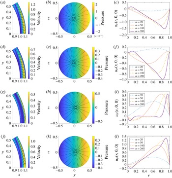
The flow of the dominant harmonic component ( $k=1$ ) in the special case of $h$ constant. The four rows show four equally spaced times through the first half-period (those during the second half-period are the reflections of these): $t=0,~\unicode[STIX]{x03C0}/4,~\unicode[STIX]{x03C0}/2$ and $3\unicode[STIX]{x03C0}/4$ , respectively. (a,d,g,j) Arrows indicate fluid velocity relative to the domain $\boldsymbol{u}^{(1)}$ and shading indicates its dimensionless magnitude on half of the midplane $z=0$ (the other half is an antisymmetric reflection). (b,e,h,k) Dimensionless pressure $p^{(1)}$ at $r=0$ (shading) and $r$ -integrated velocity $\boldsymbol{q}_{h}^{(1)}$ (arrows), projected onto a plane of constant $x$ . (c,f,i,l) Profiles of the relative velocity component $u_{\unicode[STIX]{x1D703}^{\prime }}$ along the axis $\unicode[STIX]{x1D703}^{\prime }=0$ . For all plots we used $\unicode[STIX]{x1D6FD}=6.5^{\circ }$ and $\unicode[STIX]{x1D716}=0.11$ , and in the first two columns we used $\unicode[STIX]{x1D6FC}=100$ . The velocity vectors in the first two columns are normalised so that their maximum length is the same in all plots.

We start with the special case of constant $h$ . In figure 4 we show the flow component with frequency 1 $(k=1)$ , which we expect to be much larger than the other two components ( $k=0,2$ ). We show the flow and pressure via snapshots at four different times in the different rows. The first row ( $t=0$ ) corresponds to the time when the angular velocity is maximum and the domain is moving in the direction of the positive $y$ -axis, and the subsequent rows correspond to subsequent times spaced $1/8$ period apart.

In figure 4(a,d,g,j), we show the velocity on the horizontal midplane $z=0$ and $y>0$ . In each case the fluid close to the inner wall moves in the same direction as the rotation and that near the outer wall moves in the opposite direction (with the exception of $t=\unicode[STIX]{x03C0}/2$ when the domain is not moving; figure 4 g). Note that the fact that the velocity does not go to zero at the boundary $\unicode[STIX]{x1D703}^{\prime }=\unicode[STIX]{x1D703}_{0}$ (as can be seen in (a,d,g,j) and (b,e,h,k)) is because, due to the simplification of lubrication theory, we can only impose zero flux there rather than a full no-slip condition. Close to $\unicode[STIX]{x1D703}^{\prime }=\unicode[STIX]{x1D703}_{0}$ the assumptions of lubrication theory do not hold, and the radial velocity component would be comparable to the other components.

In figure 4(b,e,h,k), we show the $r$ -integrated velocity field obtained from (3.10) and the pressure distribution on the surface $r=1$ , both projected onto a plane of constant $x$ . At $t=0$ the angular acceleration is zero, and thus the pressure is almost constant on the surface $r=0$ (figure 4 b), but the pressure gradient is much larger at the other three times, especially at $t=\unicode[STIX]{x03C0}/2$ when the angular acceleration peaks (figure 4 h). Each plot shows two circulations that are reflections of one another, which indicates that the instantaneous flow has a highly three-dimensional structure.

Figure 4(c,f,i,l) shows the velocity component $u_{\unicode[STIX]{x1D703}^{\prime }}$ along the line $\unicode[STIX]{x1D703}^{\prime }=0$ , which is a region of the positive $x$ -axis with $x=1+\unicode[STIX]{x1D716}r$ . Each line corresponds to a different value of the Womersley number $\unicode[STIX]{x1D6FC}$ . Inspection of the plots shows that, as the Womersley number increases, a progressively thinner oscillatory Stokes boundary layer forms at both walls, as expected.

Figure 5.

The steady streaming flow in the special case of a domain of constant height, shown (a) on half of the midplane $y=0$ ( $\unicode[STIX]{x1D719}^{\prime }=\unicode[STIX]{x03C0}$ ) (the other half is a symmetric reflection), (b) on the plane $r=0.2$ and (c) on the plane $r=0.8$ . The arrows indicate the relative velocity $\boldsymbol{u}^{(0)}$ and colours indicate its magnitude. The parameter values are $\unicode[STIX]{x1D6FC}=100$ , $\unicode[STIX]{x1D6FD}=6.5^{\circ }$ , $\unicode[STIX]{x1D716}=0.11$ .

In figure 5(a) we show the steady streaming flow on the vertical plane $y=0$ . We only plot the upper half of the domain since the flow is symmetric in the $x$ -axis, as can be seen by inspecting equations (3.17b ) and (3.17c ). In the outer part of the domain fluid particles move towards the midplane $z=0$ and in the inner part of the domain they move away from $z=0$ . This is consistent with what is found for a periodically rotating sphere (Repetto, Siggers & Stocchino Reference Repetto, Siggers and Stocchino2008; Colombini Reference Colombini2014), where a circulation with the same sense of rotation is found, and also with the numerical findings of Abouali et al. (Reference Abouali, Modareszadeh, Ghaffarieh and Tu2012), relative to the flow in the AC. Since the model does not capture the behaviour of the oscillatory flow close to the boundary of the domain (at $\unicode[STIX]{x1D703}^{\prime }=\unicode[STIX]{x1D703}_{0}$ ), we cannot rule out the possibility that boundary effects could produce a steady streaming in the core of the domain. The flows on the planes $r=0.2$ and $r=0.8$ are shown in figure 5(b,c). The velocity profile is almost vertical in both cases and there is very little transversal flow. Moreover, we recall that in the case of the constant-thickness domain the $r$ -integrated velocity $\boldsymbol{q}_{\mathit{h}}$ is equal to zero.

Figure 6.

Velocity magnitudes over a range of frequencies in the special case of a constant-height domain. Maximum value (over both time and space) attained by the magnitude of the velocity as a function of the Womersley number $\unicode[STIX]{x1D6FC}$ . The different line styles denote the different harmonics: $k=0$ (solid); $k=1$ (dot-dashed); and $k=2$ (dashed); and the thickness and colour show the values of $\unicode[STIX]{x1D716}$ : $\unicode[STIX]{x1D716}\approx 0.15$ (thick green); $\unicode[STIX]{x1D716}\approx 0.11$ (medium red); and $\unicode[STIX]{x1D716}\approx 0.06$ (thin blue). The amplitude is fixed at $\unicode[STIX]{x1D6FD}=6.5^{\circ }$ in each case.

In figure 6 we show the maximum dimensional value over time and space attained by the velocity for each of the harmonics as a function of the Womersley number $\unicode[STIX]{x1D6FC}$ . As expected, the magnitude of the dominant harmonic $k=1$ velocity is much larger than those of the others. Moreover, the steady streaming velocity has a significantly larger magnitude than that of the harmonic $k=2$ for large values of $\unicode[STIX]{x1D6FC}$ .

Figure 7.

As for figure 4, but for the case of the more realistic eye shape described in the introduction of § 2.1.

4.2 More realistic eye geometry

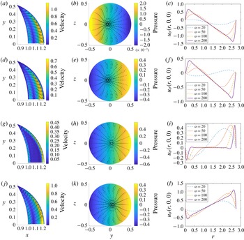
In this section we report the results obtained using the more realistic shape of the AC of the eye, shown in figure 2(c). Figure 7 is the analogy of figure 4 for this case, and mostly shows qualitatively similar findings. However, in the case of the more realistic domain shape, the velocity decreases near the periphery of the domain ( $\unicode[STIX]{x1D703}^{\prime }$ near to $\unicode[STIX]{x1D703}_{0}$ ), since the domain is thinner there. It is interesting to note that the circulations in the $r$ -integrated velocity fields that were observed in the case of the constant-height domain are still present in this case, suggesting that the flow induced by eye rotations is highly three-dimensional.

Figure 8.

Maximum dimensional value over space and time of the wall shear stress on the cornea as a function of the angular amplitude of the saccadic eye rotation $\unicode[STIX]{x1D6FD}$ in the case of the more realistic eye shape. For each value of $\unicode[STIX]{x1D6FD}$ the curve for saccades in figure 3 was used to find the corresponding value of $\unicode[STIX]{x1D6FC}$ . The lines with different thickness and colour correspond to different values of $h_{max}$ : medium red: $h_{max}=2.62$ mm ( $\unicode[STIX]{x1D716}\approx 0.11$ ); thin blue: $h_{max}=1.5$ mm ( $\unicode[STIX]{x1D716}\approx 0.06$ ); thick green: $h_{max}=3.5$ mm ( $\unicode[STIX]{x1D716}\approx 0.15$ ). The symbols refer to REM: triangles represent maximum amplitude REM and circles average REM, with their thickness and colour corresponding to maximum height of the domain considered. The three symbols for average REM cannot be distinguished as they are approximately on top of one another.

In figure 8 we plot the maximum dimensional value over space and time of the WSS on the cornea as a function of the eye rotation amplitude in the case of both saccades and REM. We compared the results for three different values of maximum thickness of the AC, within the physiological range (e.g. Jivrajka et al. Reference Jivrajka, Shammas, Boenzi, Swearingen and Shammas2008). The maximum WSS increases with the height of the domain, and, for a given domain, peaks for saccade amplitudes of around 0.15 rad or $8.6^{\circ }$ .

Figure 9.

The steady streaming flow for the more realistic domain shape. (a) Relative velocity $\boldsymbol{u}^{(0)}$ on the vertical cross-section $y=0$ . (b) The $r$ -integrated velocity, projected onto the $(y,z)$ -plane. Colours indicate velocity magnitude and arrows show magnitude and direction. The parameters are $\unicode[STIX]{x1D6FC}=100$ , $\unicode[STIX]{x1D6FD}=6.5^{\circ }$ , $\unicode[STIX]{x1D716}=0.11$ .

Figure 10.

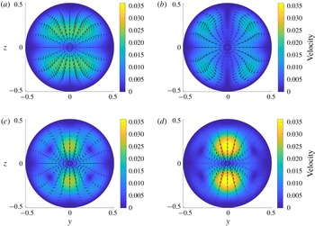
Steady streaming flow $\boldsymbol{u}^{(0)}$ for the case of realistic shape at the planes: (a) $r=0.2h/\bar{h}$ , (b) $r=0.4h/\bar{h}$ , (c) $r=0.6h/\bar{h}$ and (d) $r=0.8h/\bar{h}$ . Colours indicate velocity magnitude and arrows show magnitude and direction. The parameters are $\unicode[STIX]{x1D6FC}=100$ , $\unicode[STIX]{x1D6FD}=6.5^{\circ }$ , $\unicode[STIX]{x1D716}=0.11$ .

Figure 11.

Maximum over space and time of the magnitude of the steady streaming flow as a function of the angular amplitude of the eye rotation. The solid curves and symbols are as in figure 8. The thermal flow due to body heating is also shown (as horizontal dashed lines since they do not correspond to a particular value of $\unicode[STIX]{x1D6FD}$ ), calculated based on Canning et al. (Reference Canning, Greaney, Dewynne and Fitt2002) (see § 5 for details), coloured and having width representing thickness of the domain (as in figure 8).

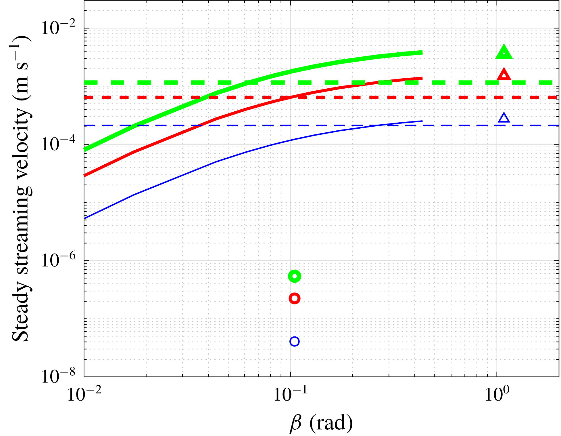
Figure 9 shows the steady streaming, which indicates similar behaviour to the constant-height case (figure 5), but in this case a closed circulation is visible in figure 9(a), which forms since the domain gets thin close to the periphery $\unicode[STIX]{x1D703}^{\prime }=\unicode[STIX]{x1D703}_{0}$ . Furthermore, the $r$ -integrated velocity is non-zero (figure 9 b), unlike in the constant-height case, meaning that the streaming flow is fully three-dimensional and there is a formation of four symmetrically arranged circulations. The flow on four equally distributed surfaces along the thickness of the domain is shown in figure 10. Close to the inner boundary of the AC, the flow has characteristics similar to those in the case of constant thickness. The steady streaming has a complicated structure, which is highly variable in the radial direction, and the flow reversal observed on the plane $y=0$ in figure 9(a) does not occur everywhere in the domain. The magnitude of the transversal flow is smaller than that on the midplane shown in figure 9(a), but it is likely to have physiological importance, as they lead to transverse mixing in the AC.

Figure 11 shows the dependence of the maximum dimensional steady streaming velocity on the saccade amplitude, with the colours corresponding to different thicknesses of the domain. Maximum steady streaming velocity increases with the saccade amplitude. The steady streaming velocity of maximum amplitude REM is also similar, whereas that of average REM is much lower. Increasing the thickness of the AC leads to higher steady streaming velocities in each case.

The results of the model are based on various assumptions, which have been discussed in § 2. In particular, we neglected the terms of order $\unicode[STIX]{x1D716}\unicode[STIX]{x1D6FD}$ , compared with terms of order $\unicode[STIX]{x1D716}$ , but also discussed cases in which the amplitude of oscillations $\unicode[STIX]{x1D6FD}$ is quite large, such as large saccades and maximum amplitude REM, which is formally out of the range of validity of our asymptotic approach. In order to verify the accuracy of our results, we have run a series of three-dimensional unsteady simulations using the commercial software COMSOL Multiphysics^®. In particular, we focused on the oscillatory component of the flow and did not consider the steady streaming. We compared our theoretical results with the numerics in terms of the $u_{\unicode[STIX]{x1D703}^{\prime }}$ velocity component along the line $\unicode[STIX]{x1D703}^{\prime }=0$ and computed the corresponding time-averaged normalised $L_{2}$ error between our model and the numerical predictions. We performed several numerical simulations varying both $\unicode[STIX]{x1D716}$ and $\unicode[STIX]{x1D6FD}$ . We find that the error is of order $\unicode[STIX]{x1D716}$ and weakly depends on $\unicode[STIX]{x1D6FD}$ for values of $\unicode[STIX]{x1D6FD}$ up to 1. These results are reassuring concerning the validity of the theory for values of $\unicode[STIX]{x1D6FD}$ of order 1, such as large saccades or REM.

5 Discussion

We have studied the flow in a thin domain performing harmonic rotations about a fixed axis, in order to investigate the flow in the AC of the eye induced by eye rotations. As mentioned in the Introduction, this is relevant to the study of nutrient and drug delivery to the tissues of the eye, and allows us to estimate the shear stresses on the cornea, which could lead to the detachment of endothelial cells.

We worked in a reference frame moving with the domain, and assumed that the aspect ratio of the AC is small, the Womersley number $\unicode[STIX]{x1D6FC}$ is large and the angular amplitude $\unicode[STIX]{x1D6FD}<1$ rad, which allowed us to reduce the governing equations to a linear system forced by the angular and the centrifugal accelerations. We considered both the case of a domain with constant thickness, for which we found a fully analytical solution, and a more realistic approximation of the AC geometry. The flow has three components: the largest oscillates with the forcing frequency, and the other two are a steady streaming component and a component that has twice the fundamental frequency.

In the cases of both a constant-height chamber and the more realistic shape, we find that the dominant frequency component of the flow has a complex three-dimensional structure, which has not been observed in previous numerical simulations of the flow in the AC (Abouali et al. Reference Abouali, Modareszadeh, Ghaffarieh and Tu2012; Modarreszadeh et al. Reference Modarreszadeh, Abouali, Ghaffarieh and Ahmadi2014). This is because in our analysis we work in a frame moving with the domain, making some of the details of the flow easier to observe, since they are not disguised by the velocities of the chamber itself. The dominant frequency component of the flow is associated with much higher velocities than the other components, and therefore contributes the majority of the WSS on the cornea. The WSS is larger for higher Womersley numbers as boundary layers develop, and it is also larger for thicker chambers. We found that WSS is maximised in the centre of the cornea (see also Abouali et al. Reference Abouali, Modareszadeh, Ghaffarieh and Tu2012), and reaches a maximum value of around $0.15$ Pa for $\unicode[STIX]{x1D6FD}\approx 8.6^{\circ }$ and $\unicode[STIX]{x1D6FC}=124$ . A direct comparison of our results with those of Abouali et al. (Reference Abouali, Modareszadeh, Ghaffarieh and Tu2012) is not possible, since we model the saccades differently: in that previous work, four saccades per period were used, whereas in our model we use two. We therefore adapted our model to use the same saccadic motion, and present the results in table 3, which show good agreement between our model and the work of both Abouali et al. (Reference Abouali, Modareszadeh, Ghaffarieh and Tu2012) and Modarreszadeh et al. (Reference Modarreszadeh, Abouali, Ghaffarieh and Ahmadi2014). The WSS values predicted by both our model and the models of Abouali et al. (Reference Abouali, Modareszadeh, Ghaffarieh and Tu2012) and also Repetto et al. (Reference Repetto, Pralits, Siggers and Soleri2015) are of a similar order of magnitude to those found to cause detachment ( ${\sim}0.1$ Pa) by Kaji et al. (Reference Kaji, Oshika, Usui and Sakakibara2005), who studied corneal endothelial cells in vitro. This suggests that higher values of WSS would be required in vivo for the corneal cells to detach. Note that the values of the WSS due to eye rotations are much larger than those produced by the buoyancy-driven flow due to temperature differences in the AC, which are about 0.0016 Pa (e.g Repetto et al. Reference Repetto, Pralits, Siggers and Soleri2015).

Table 3.

Comparison of the maximum WSS (in Pa) on the cornea calculated with the present model with the results from numerical works of Abouali et al. (Reference Abouali, Modareszadeh, Ghaffarieh and Tu2012) (saccades) and Modarreszadeh et al. (Reference Modarreszadeh, Abouali, Ghaffarieh and Ahmadi2014) (REM).

The steady streaming flow is forced by the centrifugal acceleration, and its velocity is much smaller than that of the flow oscillating with the forcing frequency, but nevertheless can have a key role in mixing processes, as it is time independent. The steady streaming flow has a complicated three-dimensional structure, which was not fully highlighted in the numerical simulations of Abouali et al. (Reference Abouali, Modareszadeh, Ghaffarieh and Tu2012) and Modarreszadeh et al. (Reference Modarreszadeh, Abouali, Ghaffarieh and Ahmadi2014), and has a non-zero $r$ -integrated velocity for a realistic shape of the domain. We note that Modarreszadeh et al. (Reference Modarreszadeh, Abouali, Ghaffarieh and Ahmadi2014) also observed smaller vortices close to the pupil boundary and next to the trabecular meshwork, which we cannot capture with our model due to our geometrical simplifications and use of lubrication theory.

In order to estimate the effective importance of the steady streaming flow on mixing in the AC, we compute the Péclet number, which measures the strength of advection over diffusion, and is given by $Pe=LU/D$ , where $D$ is the diffusion coefficient, $L$ is the radius of the AC and $U$ is characteristic velocity. With $D=10^{-9}~\text{m}^{2}~\text{s}^{-1}$ (Lide Reference Lide1996), $L=6.2$ mm and a typical value of the velocity of $5\times 10^{-4}~\text{m}~\text{s}^{-1}$ (see figure 11), we obtain $Pe\approx O(10^{3})$ . The $r$ -integrated steady streaming is much smaller, and the corresponding Péclet number is of order $10^{2}$ . In both cases it is clear that advection largely dominates over diffusion, and confirms that eye rotations have a key role in governing transport processes in the AC. An effect that could be potentially relevant for transport processes in the AC, and that has been neglected in the present work, is shear-augmented diffusion via a ‘Taylor dispersion’ mechanism. We leave the consideration of such an effect to possible future work.

Besides eye rotations, the other mechanism that is known to produce a flow that significantly contributes to fluid mixing is the temperature gradient across the AC, since it also leads to the generation of a steady flow. To compare the steady streaming flow during saccades with the thermal flow we make use of the results of Canning et al. (Reference Canning, Greaney, Dewynne and Fitt2002), who developed an idealised model in which the geometry of the AC was approximated as a spherical cap to derive an analytical expression for the thermal flow. This showed that the flow is directed along the vertical planes. The maximum magnitude of the fluid velocity was found to be

(5.1)

$$\begin{eqnarray}u_{T,max}={\displaystyle \frac{\unicode[STIX]{x0394}T\unicode[STIX]{x1D70C}g\unicode[STIX]{x1D6FC}_{T}h_{max}^{2}\sqrt{3}}{216\unicode[STIX]{x1D708}}},\end{eqnarray}$$

where $\unicode[STIX]{x0394}T$ is the temperature difference between the cornea and the iris, $\unicode[STIX]{x1D6FC}_{T}=3\times 10^{-4}~\text{K}^{-1}$ is the coefficient of thermal expansion, $g$ is gravitational acceleration, $\unicode[STIX]{x1D70C}$ and $\unicode[STIX]{x1D708}$ are fluid density and kinematic viscosity, respectively, and $h_{max}$ is the maximum thickness of the AC (see table 1). With $\unicode[STIX]{x0394}T=3$ K, we estimate $u_{T,max}=6.47\times 10^{-4}~\text{m}~\text{s}^{-1}$ . Tweedy et al. (Reference Tweedy, Pralits, Repetto and Soleri2017) used a similar method and, using their code with the same geometry as used here, they found a maximum velocity of $6.84\times 10^{-4}~\text{m}~\text{s}^{-1}$ , while Repetto et al. (Reference Repetto, Pralits, Siggers and Soleri2015) used a numerical method for a slightly different geometry and found a maximum velocity of $5.92\times 10^{-4}~\text{m}~\text{s}^{-1}$ for $\unicode[STIX]{x0394}T=3$ K, which are both close to the value derived analytically from (5.1). We therefore assume that (5.1) provides a sufficiently accurate estimate for our purposes. We compare the thermal flow and the steady streaming flow induced by eye rotations in figure 11, which shows that the steady flow induced by eye rotations has the same order of magnitude for large saccades and REM. Thus the two flows both effectively contribute to mixing in the AC.

During the night, thermally driven flow becomes insignificant, and, aside from shape changes of the AC, the mechanisms driving flow are the REM and aqueous secretion. The maximum magnitude of the latter is ${\approx}5.89\times 10^{-5}~\text{m}~\text{s}^{-1}$ (Repetto et al. Reference Repetto, Pralits, Siggers and Soleri2015) at the pupil and its average velocity is ${\approx}8\times 10^{-6}~\text{m}~\text{s}^{-1}$ , which are both significantly smaller than the steady streaming flow found in the work. This provides confirming evidence for the hypothesis of Maurice (Reference Maurice1998), which is that REM could promote mixing in the otherwise almost stagnant aqueous humour in order to maintain the nutrient supply to the cornea.

This work neglects any interactions between the flow induced by eye rotations and the other flow mechanisms in the AC. For small fluid velocities, due to linearity, the total flow may be approximated as the sum of the flow due to saccades, that due to secretion and drainage of the aqueous humour and the thermally driven flow. However, any flow due to shape deformations in the AC would be fully interactive with the other flows and would thus require a separate study.

To summarise, we find good agreement with previous numerical solutions and highlight characterestics of the flow that were not previously described. We show that the flow induced by eye rotations is a significant part of the aqueous humour dynamics and an important player in mixing processes. Finally, we remark that the model developed here could be useful for other applications involving oscillating thin domains.

Acknowledgements

This work was financially supported by Ophtec BV (the Netherlands). The authors thank Professor F. Grillo for drawing figure 1 and P. Soleri for many useful suggestions.

Appendix A. Definitions of the functions introduced in § 3

We report functions appearing in the expressions used in § 3.

A.1 Harmonic $k=0$

(A 1a )

$$\begin{eqnarray}\displaystyle & \displaystyle A_{0}(r,h)={\displaystyle \frac{\unicode[STIX]{x1D716}\unicode[STIX]{x1D6FC}^{2}}{2}}\left(r(r-h)-{\displaystyle \frac{\unicode[STIX]{x1D716}r}{3}}(r^{2}-h^{2})\right), & \displaystyle\end{eqnarray}$$

(A 1b )

$$\begin{eqnarray}\displaystyle & \displaystyle B_{0}(r,h)={\displaystyle \frac{\unicode[STIX]{x1D6FD}\unicode[STIX]{x1D716}\unicode[STIX]{x1D6FC}^{2}}{16}}(rh-r^{2}), & \displaystyle\end{eqnarray}$$

(A 1c )

$$\begin{eqnarray}\displaystyle & \displaystyle \unicode[STIX]{x1D6FE}_{0}(h)=\int _{0}^{h}(1+\unicode[STIX]{x1D716}r)A_{0}(r,h)\,\text{d}r={\displaystyle \frac{\unicode[STIX]{x1D6FD}\unicode[STIX]{x1D716}\unicode[STIX]{x1D6FC}^{2}h^{3}}{180\unicode[STIX]{x1D6FD}}}(4\unicode[STIX]{x1D716}^{2}h^{2}-15), & \displaystyle\end{eqnarray}$$

(A 1d )

$$\begin{eqnarray}\displaystyle & \displaystyle \unicode[STIX]{x1D6FF}_{0}(h)=\int _{0}^{h}(1+\unicode[STIX]{x1D716}r)B_{0}(r,h)\,\text{d}r={\displaystyle \frac{\unicode[STIX]{x1D6FD}\unicode[STIX]{x1D716}\unicode[STIX]{x1D6FC}^{2}}{96}}\left({\displaystyle \frac{\unicode[STIX]{x1D716}h^{4}}{2}}+h^{3}\right). & \displaystyle\end{eqnarray}$$

A.2 Harmonic $k=1$

(A 2a )

$$\begin{eqnarray}\displaystyle & \displaystyle A_{1}(r,h)={\displaystyle \frac{\text{i}}{\unicode[STIX]{x1D716}}}\left({\displaystyle \frac{\sin ar(\unicode[STIX]{x1D716}h+\cos ah-1)}{\sin ah}}-\cos ar-(\unicode[STIX]{x1D716}r-1)\right), & \displaystyle\end{eqnarray}$$

(A 2b )

$$\begin{eqnarray}\displaystyle & \displaystyle B_{1}(r,h)={\displaystyle \frac{1}{2\unicode[STIX]{x1D716}}}\left({\displaystyle \frac{\sin ar(\unicode[STIX]{x1D716}h-\cos ah+1)}{\sin ah}}+\cos ar-(\unicode[STIX]{x1D716}r+1)\right), & \displaystyle\end{eqnarray}$$

(A 2c )

$$\begin{eqnarray}\displaystyle & \displaystyle \unicode[STIX]{x1D6FE}_{1}(h)=-\text{i}\left({\displaystyle \frac{\unicode[STIX]{x1D716}h^{3}}{3}}-{\displaystyle \frac{h}{\unicode[STIX]{x1D716}}}-{\displaystyle \frac{\unicode[STIX]{x1D716}h}{a^{2}}}+{\displaystyle \frac{2-2\cos ah+\unicode[STIX]{x1D716}^{2}h^{2}\cos ah}{\unicode[STIX]{x1D716}a\sin ah}}\right), & \displaystyle\end{eqnarray}$$

(A 2d )

$$\begin{eqnarray}\displaystyle & \hspace{-12.0pt}\displaystyle \unicode[STIX]{x1D6FF}_{1}(h)=-{\displaystyle \frac{1}{2}}\!\left({\displaystyle \frac{\unicode[STIX]{x1D716}h^{3}}{3}}+h^{2}+{\displaystyle \frac{h}{\unicode[STIX]{x1D716}}}-{\displaystyle \frac{h\unicode[STIX]{x1D716}}{a^{2}}}+{\displaystyle \frac{\unicode[STIX]{x1D716}(\unicode[STIX]{x1D716}h^{2}+2h)\cos ah-2\unicode[STIX]{x1D716}h+2(\cos ah-1)}{\unicode[STIX]{x1D716}a\sin ah}}\right)\!,\qquad & \displaystyle\end{eqnarray}$$

where

$a=\sqrt{-\text{i}}\unicode[STIX]{x1D716}\unicode[STIX]{x1D6FC}=\pm (1-\text{i})\unicode[STIX]{x1D716}\unicode[STIX]{x1D6FC}/\sqrt{2}$ .

The components of the $r$ -integrated velocity are

(A 3)

$$\begin{eqnarray}\displaystyle & \displaystyle q_{\unicode[STIX]{x1D703}}^{(1)}=\unicode[STIX]{x1D6FF}_{1}(r)\left(1-{\displaystyle \frac{\sin ^{2}\unicode[STIX]{x1D703}_{0}}{1-\cos \unicode[STIX]{x1D703}_{0}}}{\displaystyle \frac{1-\cos \unicode[STIX]{x1D703}^{\prime }}{\sin ^{2}\unicode[STIX]{x1D703}^{\prime }}}\right)\sin \unicode[STIX]{x1D719}^{\prime }, & \displaystyle\end{eqnarray}$$

(A 4)

$$\begin{eqnarray}\displaystyle & \displaystyle q_{\unicode[STIX]{x1D719}}^{(1)}=\unicode[STIX]{x1D6FF}_{1}(r)\left(\cos \unicode[STIX]{x1D703}^{\prime }-{\displaystyle \frac{\sin ^{2}\unicode[STIX]{x1D703}_{0}}{1-\cos \unicode[STIX]{x1D703}_{0}}}{\displaystyle \frac{1-\cos \unicode[STIX]{x1D703}^{\prime }}{\sin ^{2}\unicode[STIX]{x1D703}^{\prime }}}\right)\cos \unicode[STIX]{x1D719}^{\prime }. & \displaystyle\end{eqnarray}$$

A.3 Harmonic $k=2$

(A 5)

$$\begin{eqnarray}\displaystyle & \displaystyle A_{2}(r,h)={\displaystyle \frac{\text{i}}{2\unicode[STIX]{x1D716}}}\left({\displaystyle \frac{\sin br(\unicode[STIX]{x1D716}h+\cos bh-1)}{\sin bh}}-\cos br-(\unicode[STIX]{x1D716}r-1)\right), & \displaystyle\end{eqnarray}$$

(A 6)

$$\begin{eqnarray}\displaystyle & \displaystyle \quad \unicode[STIX]{x1D6FE}_{2}(r,h)=-{\displaystyle \frac{\text{i}}{2}}\left({\displaystyle \frac{\unicode[STIX]{x1D716}h^{3}}{3}}-{\displaystyle \frac{h}{\unicode[STIX]{x1D716}}}-{\displaystyle \frac{\unicode[STIX]{x1D716}h}{b^{2}}}+{\displaystyle \frac{2-2\cos bh+\unicode[STIX]{x1D716}^{2}h^{2}\cos bh}{\unicode[STIX]{x1D716}b\sin bh}}\right), & \displaystyle\end{eqnarray}$$

(A 7)

$$\begin{eqnarray}\displaystyle & \displaystyle B_{2}(r,h)={\displaystyle \frac{\text{i}\unicode[STIX]{x1D6FD}}{16\unicode[STIX]{x1D716}}}\left(\sin br{\displaystyle \frac{1-\cos bh}{\sin bh}}+\cos br-1\right), & \displaystyle\end{eqnarray}$$

(A 8)

$$\begin{eqnarray}\displaystyle & \displaystyle \unicode[STIX]{x1D6FF}_{2}(r,h)=-{\displaystyle \frac{\text{i}\unicode[STIX]{x1D6FD}}{16\unicode[STIX]{x1D716}}}\left({\displaystyle \frac{(2+\unicode[STIX]{x1D716}h)(\cos bh-1)}{b\sin bh}}+h+{\displaystyle \frac{\unicode[STIX]{x1D716}h^{2}}{2}}\right), & \displaystyle\end{eqnarray}$$

where $b=\sqrt{-2\text{i}}\unicode[STIX]{x1D716}\unicode[STIX]{x1D6FC}=\pm (1-\text{i})\unicode[STIX]{x1D716}\unicode[STIX]{x1D6FC}$ .

References

Abouali, O., Modareszadeh, A., Ghaffarieh, A. & Tu, J. 2012 Investigation of saccadic eye movement effects on the fluid dynamic in the anterior chamber. J. Biomech. Engng 134 (2), 021002.10.1115/1.4005762Google Scholar

Batchelor, G. K. 1967 An Introduction to Fluid Dynamics. Cambridge University Press.Google Scholar

Becker, W. 1989 Metrics. In The Neurobiology of Saccadic Eye Movements (ed. Wurtz, R. H. & Goldberg, M. E.), pp. 13–67. Elsevier Science.Google Scholar

Beswick, J. A. & McCulloch, C. 1956 Effect of hyaluronidase on the viscosity of the aqueous humour. Brit. J. Ophthalmol. 40 (9), 545–548.10.1136/bjo.40.9.545Google Scholar

Blondeaux, P. & Vittori, G. 1994 Wall imperfections as a triggering mechanism for Stokes-layer transition. J. Fluid Mech. 264, 107–135.10.1017/S0022112094000601Google Scholar

Bonfiglio, A., Lagazzo, A., Repetto, R. & Stocchino, A. 2015 An experimental model of vitreous motion induced by eye rotations. Eye Vis. 2 (1), 1–10.10.1186/s40662-015-0020-8Google Scholar

Bonfiglio, A., Repetto, R., Siggers, J. H. & Stocchino, A. 2013 Investigation of the motion of a viscous fluid in the vitreous cavity induced by eye rotations and implications for drug delivery. Phys. Med. Biol. 58 (6), 1969–1982.10.1088/0031-9155/58/6/1969Google Scholar

Boushehrian, H. H., Abouali, O., Jafarpur, K., Ghaffarieh, A. & Ahmadi, G. 2016 Relationship between saccadic eye movements and formation of the Krukenberg’s spindle: a CFD study. Math. Med. Biol. 34 (3), 293–312.Google Scholar

Brubaker, R. F. 1991 Flow of aqueous humor in humans [The Friedenwald Lecture]. Invest. Ophthalmol. Vis. Sci. 32 (13), 3145–3166.Google Scholar

Canning, C. R., Greaney, M. J., Dewynne, J. N. & Fitt, A. 2002 Fluid flow in the anterior chamber of a human eye. IMA J. Math. Appl. Med. Biol. 19, 31–60.10.1093/imammb/19.1.31Google Scholar

Colombini, M. 2014 Axisymmetric flow within a torsionally oscillating sphere. Phys. Fluids 26 (2), 023602.10.1063/1.4866812Google Scholar

David, T., Smye, S., Dabbs, T. & James, T. 1998 A model for the fluid motion of vitreous humour of the human eye during saccadic movement. Phys. Med. Biol. 43, 1385–1399.10.1088/0031-9155/43/6/001Google Scholar

Dvoriashyna, M., Repetto, R., Romano, M. R. & Tweedy, J. H. 2017 Aqueous humour flow in the posterior chamber of the eye and its modifications due to pupillary block and iridotomy. Math. Med. Biol. https://doi.org/10.1093/imammb/dqx012.Google Scholar

Fitt, A. D. & Gonzalez, G. 2006 Fluid mechanics of the human eye: aqueous humour flow in the anterior chamber. Bull. Math. Biol. 68 (1), 53–71.10.1007/s11538-005-9015-2Google Scholar

Friedland, A. B. 1978 A hydrodynamic model of aqueous flow in the posterior chamber of the eye. Bull. Math. Biol. 40, 223–235.10.1007/BF02461437Google Scholar

Helmholtz, H. 1909 Handbuch der physiologischen Optik, 3rd edn. University of Michigan Library.Google Scholar

Heys, J. J. & Barocas, V. H. 2002 A Boussinesq model of natural convection in the human eye and formation of Krunberg’s spindle. Ann. Biomed. Engng 30, 392–401.10.1114/1.1477447Google Scholar

Jivrajka, R., Shammas, M. C., Boenzi, T., Swearingen, M. & Shammas, H. J. 2008 Variability of axial length, anterior chamber depth, and lens thickness in the cataractous eye. J. Cataract Refract. Surg. 34 (2), 289–294.10.1016/j.jcrs.2007.10.015Google Scholar

Kaji, Y., Oshika, T., Usui, T. & Sakakibara, J. 2005 Effect of shear stress on attachment of corneal endothelial cells in association with corneal endothelial cell loss after laser iridotomy. Cornea 24 (8), S55–S58.10.1097/01.ico.0000178735.27674.52Google Scholar

Lide, D. R.(Ed.) 1996 CRC Handbook of Chemistry and Physics, 77th edn. CRC Press.Google Scholar

Maurice, D. M. 1998 The von Sallmann lecture 1996: an ophthalmological explanation of REM sleep. Exp. Eye Res. 66 (2), 139–145.10.1006/exer.1997.0444Google Scholar

Meskauskas, J., Repetto, R. & Siggers, J. H. 2011 Oscillatory motion of a viscoelastic fluid within a spherical cavity. J. Fluid Mech. 685, 1–22.10.1017/jfm.2011.263Google Scholar

Meskauskas, J., Repetto, R. & Siggers, J. H. 2012 Shape change of the vitreous chamber influences retinal detachment and reattachment processes: is mechanical stress during eye rotations a factor? Invest. Ophthalmol. Visual Sci. 53 (10), 6271–6281.10.1167/iovs.11-9390Google Scholar

Modarreszadeh, S., Abouali, O., Ghaffarieh, A. & Ahmadi, G. 2014 Physiology of aqueous humor dynamic in the anterior chamber due to rapid eye movement. Physiol. Behav. 135, 112–118.10.1016/j.physbeh.2014.05.017Google Scholar

Repetto, R., Pralits, J. O., Siggers, J. H. & Soleri, P. 2015 Phakic iris-fixated intraocular lens placement in the anterior chamber: effects on aqueous flow. Invest. Ophthalmol. Visual Sci. 56 (5), 3061–3068.10.1167/iovs.14-16118Google Scholar

Repetto, R., Siggers, J. H. & Stocchino, A. 2008 Steady streaming within a periodically rotating sphere. J. Fluid Mech. 608, 71–80.10.1017/S002211200800222XGoogle Scholar

Repetto, R., Siggers, J. H. & Stocchino, A. 2010 Mathematical model of flow in the vitreous humor induced by saccadic eye rotations: effect of geometry. Biomech. Model. Mechanobiol. 9 (1), 65–76.10.1007/s10237-009-0159-0Google Scholar

Repetto, R., Stocchino, A. & Cafferata, C. 2005 Experimental investigation of vitreous humour motion within a human eye model. Phys. Med. Biol. 50, 4729–4743.10.1088/0031-9155/50/19/021Google Scholar

Silver, D. M. & Quigley, H. A. 2004 Aqueous flow through the iris-lens channel: estimates of the differential pressure between the anterior and the posterior chambers. J. Glaucoma 13 (2), 100–107.10.1097/00061198-200404000-00004Google Scholar

Sommer, A., Tielsch, J. M., Katz, J., Quigley, H. A., Gottsch, J. D., Javitt, J. & Singh, K. 1991 Relationship between intraocular pressure and primary open angle glaucoma among white and black Americans. Arch. Ophthalmol. 109 (8), 1090–1095.10.1001/archopht.1991.01080080050026Google Scholar

Takahashi, K. & Atsumi, Y. 1997 Precise measurement of individual rapid eye movements in REM sleep of humans. Sleep 20 (9), 743–752.10.1093/sleep/20.9.743Google Scholar

Tweedy, J. H., Pralits, J. O., Repetto, R. & Soleri, P. 2017 Flow in the anterior chamber of the eye with an implanted iris-fixated artificial lens. Math. Med. Biol. 35 (3), 363–385.10.1093/imammb/dqx007Google Scholar

Urtti, A. 2006 Challenges and obstacles of ocular pharmacokinetics and drug delivery. Adv. Drug Deliv. Rev. 58 (11), 1131–1135.10.1016/j.addr.2006.07.027Google Scholar

Villamarin, A., Roy, S., Hasballa, R., Vardoulis, O., Reymond, P. & Stergiopulos, N. 2012 3D simulation of the aqueous flow in the human eye. Med. Engng Phys. 34, 1462–1470.10.1016/j.medengphy.2012.02.007Google Scholar

Figure 1.Sketch of a cross-section of the human eye.

Figure 2.(a) Sketch of the eye, showing the eyeball (large sphere) and the domain representing the AC attached to the sphere on the right. Sketch of the coordinate systems ${\mathcal{C}}$ and ${\mathcal{C}}^{\prime }$. Cross-sections of the domains considered: (b) idealised constant-height domain; (c) more realistic representation of the AC geometry.

Table 1.Geometrical characteristics of the domain and fluid properties.

Figure 3.Relationship between the Womersley number $\unicode[STIX]{x1D6FC}$ and the amplitude of rotations $\unicode[STIX]{x1D6FD}$ for saccadic eye rotations (curve), average REM (circle) and maximum amplitude REM (triangle) (Modarreszadeh et al.2014).

Table 2.Typical values of the dimensionless parameters, with $\unicode[STIX]{x1D716}\approx 0.11$ in all cases.

Figure 4.The flow of the dominant harmonic component ($k=1$) in the special case of $h$ constant. The four rows show four equally spaced times through the first half-period (those during the second half-period are the reflections of these):$t=0,~\unicode[STIX]{x03C0}/4,~\unicode[STIX]{x03C0}/2$ and $3\unicode[STIX]{x03C0}/4$, respectively. (a,d,g,j) Arrows indicate fluid velocity relative to the domain $\boldsymbol{u}^{(1)}$ and shading indicates its dimensionless magnitude on half of the midplane $z=0$ (the other half is an antisymmetric reflection). (b,e,h,k) Dimensionless pressure $p^{(1)}$ at $r=0$ (shading) and $r$-integrated velocity $\boldsymbol{q}_{h}^{(1)}$ (arrows), projected onto a plane of constant $x$. (c,f,i,l) Profiles of the relative velocity component $u_{\unicode[STIX]{x1D703}^{\prime }}$ along the axis $\unicode[STIX]{x1D703}^{\prime }=0$. For all plots we used $\unicode[STIX]{x1D6FD}=6.5^{\circ }$ and $\unicode[STIX]{x1D716}=0.11$, and in the first two columns we used $\unicode[STIX]{x1D6FC}=100$. The velocity vectors in the first two columns are normalised so that their maximum length is the same in all plots.

Figure 5.The steady streaming flow in the special case of a domain of constant height, shown (a) on half of the midplane $y=0$ ($\unicode[STIX]{x1D719}^{\prime }=\unicode[STIX]{x03C0}$) (the other half is a symmetric reflection), (b) on the plane $r=0.2$ and (c) on the plane $r=0.8$. The arrows indicate the relative velocity $\boldsymbol{u}^{(0)}$ and colours indicate its magnitude. The parameter values are $\unicode[STIX]{x1D6FC}=100$, $\unicode[STIX]{x1D6FD}=6.5^{\circ }$, $\unicode[STIX]{x1D716}=0.11$.

Figure 6.Velocity magnitudes over a range of frequencies in the special case of a constant-height domain. Maximum value (over both time and space) attained by the magnitude of the velocity as a function of the Womersley number $\unicode[STIX]{x1D6FC}$. The different line styles denote the different harmonics: $k=0$ (solid); $k=1$ (dot-dashed); and $k=2$ (dashed); and the thickness and colour show the values of $\unicode[STIX]{x1D716}$: $\unicode[STIX]{x1D716}\approx 0.15$ (thick green); $\unicode[STIX]{x1D716}\approx 0.11$ (medium red); and $\unicode[STIX]{x1D716}\approx 0.06$ (thin blue). The amplitude is fixed at $\unicode[STIX]{x1D6FD}=6.5^{\circ }$ in each case.

Figure 7.As for figure 4, but for the case of the more realistic eye shape described in the introduction of § 2.1.

Figure 8.Maximum dimensional value over space and time of the wall shear stress on the cornea as a function of the angular amplitude of the saccadic eye rotation $\unicode[STIX]{x1D6FD}$ in the case of the more realistic eye shape. For each value of $\unicode[STIX]{x1D6FD}$ the curve for saccades in figure 3 was used to find the corresponding value of $\unicode[STIX]{x1D6FC}$. The lines with different thickness and colour correspond to different values of $h_{max}$: medium red: $h_{max}=2.62$ mm ($\unicode[STIX]{x1D716}\approx 0.11$); thin blue: $h_{max}=1.5$ mm ($\unicode[STIX]{x1D716}\approx 0.06$); thick green: $h_{max}=3.5$ mm ($\unicode[STIX]{x1D716}\approx 0.15$). The symbols refer to REM: triangles represent maximum amplitude REM and circles average REM, with their thickness and colour corresponding to maximum height of the domain considered. The three symbols for average REM cannot be distinguished as they are approximately on top of one another.

Figure 9.The steady streaming flow for the more realistic domain shape. (a) Relative velocity $\boldsymbol{u}^{(0)}$ on the vertical cross-section $y=0$. (b) The $r$-integrated velocity, projected onto the $(y,z)$-plane. Colours indicate velocity magnitude and arrows show magnitude and direction. The parameters are $\unicode[STIX]{x1D6FC}=100$, $\unicode[STIX]{x1D6FD}=6.5^{\circ }$, $\unicode[STIX]{x1D716}=0.11$.

Figure 10.Steady streaming flow $\boldsymbol{u}^{(0)}$ for the case of realistic shape at the planes: (a) $r=0.2h/\bar{h}$, (b) $r=0.4h/\bar{h}$, (c) $r=0.6h/\bar{h}$ and (d) $r=0.8h/\bar{h}$. Colours indicate velocity magnitude and arrows show magnitude and direction. The parameters are $\unicode[STIX]{x1D6FC}=100$, $\unicode[STIX]{x1D6FD}=6.5^{\circ }$, $\unicode[STIX]{x1D716}=0.11$.

Figure 11.Maximum over space and time of the magnitude of the steady streaming flow as a function of the angular amplitude of the eye rotation. The solid curves and symbols are as in figure 8. The thermal flow due to body heating is also shown (as horizontal dashed lines since they do not correspond to a particular value of $\unicode[STIX]{x1D6FD}$), calculated based on Canning et al. (2002) (see § 5 for details), coloured and having width representing thickness of the domain (as in figure 8).

Table 3.Comparison of the maximum WSS (in Pa) on the cornea calculated with the present model with the results from numerical works of Abouali et al. (2012) (saccades) and Modarreszadeh et al. (2014) (REM).

Article contents

Oscillatory and steady streaming flow in the anterior chamber of the moving eye

Abstract

JFM classification

Information

1 Introduction

2 Formulation of the problem

2.1 Geometry of the domain

2.2 Eye rotations

2.3 Derivation of the governing equations

3 Solution

3.1 Decomposition of the solution

3.2 Derivation of the equation for the pressure

3.3 Separation of variables and solution for the case of constant $h$

3.3.1 Dominant frequency component ( $k=1$ )

3.3.2 Steady streaming ( $k=0$ ) and double frequency ( $k=2$ ) components

4 Results

4.1 Constant-height domain

4.2 More realistic eye geometry

5 Discussion

Acknowledgements

Appendix A. Definitions of the functions introduced in § 3

A.1 Harmonic $k=0$

A.2 Harmonic $k=1$

A.3 Harmonic $k=2$

References

Save article to Kindle

Save article to Dropbox

Save article to Google Drive

Reply to: Submit a response

Your details

You have entered the maximum number of contributors

Conflicting interests