2.1 Credit-to-GDP gaps and end-of-sample problem

BCBS (2010) provided guidance to national authorities on implementing the CCyB. Countries are advised to calculate the credit-to-GDP gap using the Hodrick and Prescott (Reference Hodrick and Prescott1980, Reference Hodrick and Prescott1997) filter. This filter defines the trend such as to minimize the following penalty function:

(1) \begin{equation} \underset {\text{ }\left \{ \tau _{t}\right \} _{t=1}^{t^{\prime }}}{arg\,\, min }\sum _{t=1}^{t^{\prime }}(y_{t}-\tau _{t})^{2}+\lambda \sum _{t=2}^{t^{\prime }-1}\left [ (\tau _{t+1}-\tau _{t})-(\tau _{t}-\tau _{t-1})\right ] ^{2},t^{\prime }\leqslant T \end{equation}

where $y_{t}$ is the time series (i.e., the credit-to-GDP ratio) and $\tau _{t}$ its trend; $\lambda$ is the smoothing parameter (the bigger $\lambda$ is, the smoother the trend). The smoothing parameter used to generate the BCG is set to $\lambda =400,000,$ in accordance with the duration of the credit cycle, which can extend up to four decades (Borio and Lowe (Reference Borio and Lowe2002), Drehmann et al. (Reference Drehmann, Borio, Gambacorta, Jiminez and Trucharte2010), Drehmann and Juselius (Reference Drehmann and Juselius2014)). Then, the BCG is given by:

(2) \begin{equation} BCG_{t^{\prime }}=y_{t^{\prime }}-\tau _{t^{\prime }}. \end{equation}

Equation (1) corresponds to the one-sided HP filter. The trend value for a given period $t^{\prime }\lt T$ is estimated using data up to period $t^{\prime }$ (i.e., only with past and current observations) to account for the limited information available in real time.Footnote ⁵ In contrast, the two-sided HP filter uses all past and future values, relative to $t^{\prime }$ , which are available. Consequently, the two-sided approach provides an ex-post trend estimation. Drehmann and Juselius (Reference Drehmann and Juselius2014) have shown that, at short horizons, the two-sided credit-to-GDP gap outperforms one-sided approach in predicting banking crises. However, from an operational perspective, only the one-sided approach captures the real-time environment that policymakers face when making decisions.

Intrinsically, one-sided estimates face an end-of-sample problem: estimates are subject to ex-post revisions when new data become available. This problem has been extensively discussed in the literature (Canova (Reference Canova1998), Orphanides and van Norden (Reference Orphanides and van Norden2002)). Kaiser and Maravall (Reference Kaiser and Maravall1999, Reference Kaiser and Maravall2001) find that extending a time series with accurate forecasts reduces the disparity between real-time cycle estimates and their ex-post estimations.

Forecast-augmented credit-to-GDP gaps have thus emerged as a potential solution to mitigate the end-of-sample problem. Gerdrup et al. (Reference Gerdrup, Kvinlog and Schaanning2013), Valinskytė and Rupeika (Reference Valinskytė and Rupeika2015), Jokipii et al. (Reference Jokipii, Nyffeler and Riederer2020) and Škrinjarić (Reference Škrinjarić2022) examine Norway, Lithuania, Switzerland and Croatia respectively to investigate the relevance of forecast-augmented credit-to-GDP gaps as credit indicators within the CCyB rate decision-making framework.Footnote ⁶ Gersl and Mitterling (Reference Gersl and Mitterling2021) provide a broader analysis considering a panel of 56 countries. The conclusions are rather mixed, as Gersl and Mitterling (Reference Gersl and Mitterling2021) conclude that forecast-augmented credit-to-GDP gaps do not provide additional valuable information to predict banking crises in advanced countries but only in emerging countries.

In the existing literature, ARIMA models have traditionally been the primary forecasting method used to generate forecast-augmented credit-to-GDP gaps. However, these models may not adequately account for the long-lasting cyclical components that characterize credit-to-GDP ratio dynamics. In this paper, we turn to SSA, an “all-in-one” method that decomposes and forecasts time series, enabling a more comprehensive consideration of the underlying characteristics of credit-to-GDP ratios. Furthermore, we employ SSA to introduce a new credit metric, termed the predicted credit-to-GDP gaps.

2.2 Singular spectrum analysis: an overview

SSA provides trend-cycle decompositions. In addition, SSA is a powerful tool for time series forecasting. There are two distinct algorithms available for implementing SSA forecasting: recurrent forecasting and vector forecasting (Golyandina and Korobeynikov (Reference Golyandina and Korobeynikov2014)). While vector forecasting generally offers more robust forecasts compared to recurrent forecasting, the relative performance of these two algorithms depends on factors such as sample size and forecast horizon (Ghodsi et al. (Reference Ghodsi, Hassani, Rahmani and Silva2018)). In this paper, we conduct forecasting exercises over various horizons, using real-time data (i.e., employing a one-sided approach).Footnote ⁷ This approach involves utilizing different sample sizes. Consequently, we use both forecasting algorithms: recurrent forecasting serves as the baseline, while vector forecasting is employed for robustness checks.

We need first to present the way we proceed to assess credit gaps by SSA. We decompose the time series $\left ( y_{t}\right ) _{t=1}^{T}$ (e.g., the credit-to-GDP ratio) into 3 components: the long-term secular trend, the cyclical component and the irregular component. SSA is a 2 stages procedure (see Golyandina et al. (Reference Golyandina, Nekrutkin and Zhigljavsky2001) and Golyandina and Zhigljavsky (Reference Golyandina and Zhigljavsky2013) for details) that can provide such decomposition. Stage 1 corresponds to the decomposition stage. Stage 2 corresponds to the reconstruction stage. Two parameters must be set to implement SSA: ( $1$ ) the window length $L$ of the trajectory matrix in the decomposition stage and ( $2$ ) the grouping method of the elementary matrices in the reconstruction stage.

1. 1. The decomposition stage rely on the trajectory matrix of the time series, obtained by mapping $\left ( y_{t}\right ) _{t=1}^{T}$ into a sequence of $K$ lagged vectors of size $L$ .Footnote ⁸ Therefore, we have to determine the window length $L$ ( $1\lt L\lt T$ ). We follow the common practice recommended by Elsner and Tsonis (Reference Elsner and Tsonis1996), setting $L=T/4.$ Footnote ⁹ Then the trajectory matrix is decomposed into $L$ elementary matrices by singular value decomposition (SVD).

2. 2. The reconstruction stage proceed first by grouping the $L$ elementary matrices into 3 components. We proceed as in Bouvatier et al. (Reference Bouvatier, Delatte and Rehault2022) for the grouping. The initial elementary matrix obtained from the SVD captures the long-term secular trend, representing the general tendency. The irregular component, characterized by high-frequency fluctuations with periodicities of less than 1.5 years (i.e., 6 quarters), is identified through an automatic grouping of elementary matrices (with a frequency cut-off set at $ 1/6=0.1666$ ). Following this, we deduce the elementary matrices associated with the cyclical component.Footnote ¹⁰ Last, the reconstruction stage transforms the 3 groups of elementary matrices into 3 time series $\tilde {y}_{t}^{(j)}$ ( $j=1,2,3$ ) of length $T$ : the long-term secular trend, the cyclical component and the irregular component.

We implement SSA using real-time data and also apply it in a two-sided setting for comparative purposes. Additionally, we assess the suitability of our selected combination of window length and grouping method in capturing the cyclical component of the credit-to-GDP ratio. First, we examine alternative window lengths, specifically $L=$ $T/3$ and $T/2$ . According to Golyandina et al. (Reference Golyandina, Nekrutkin and Zhigljavsky2001) and Golyandina and Zhigljavsky (Reference Golyandina and Zhigljavsky2013), setting $L=$ $T/2$ results in the largest trajectory matrix, thereby providing the most precise decomposition. However, since the trend component is captured by the first elementary matrix, increasing $L$ results in a smoother trend and, in turn, a larger cyclical component. This may lead to the undesirable inclusion of part of the trend within the cyclical component. Following the general recommendation of Elsner and Tsonis (Reference Elsner and Tsonis1996), we find that setting $L=T/4$ produces credit-to-GDP gaps with an average magnitude comparable to those obtained using the HP filter (i.e., the Basel credit gap, see Table 1 & Figure 1). By contrast, alternative values ( $L=$ $T/3$ and $T/2$ ) result in larger cycles. We therefore conclude that longer window lengths (e.g., $L=$ $T/3$ or $T/2$ ) may excessively smooth the trend, potentially reducing the reliability of the decomposition.

Table 1.

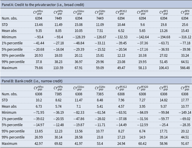
Descriptive statistics on credit-to-GDP gap

Variable definitions: ${ CY}^{{ HPos}}_{{ gap}}$ = credit-to-GDP gap computed using a one-sided HP filter; ${ CY}^{{ HPts}}_{{ gap}}$ indicates the credit-to-GDP gap is obtained via two-sided HP filter; ${ CY}^{{ SSAos}}_{{ gap}}$ via one-sided SSA; ${ CY}^{{ SSAts}}_{{ gap}}$ via two-sided SSA. ${ CY}^{{ RFA20}}_{{ gap}}$ : forecast-augmented credit-to-GDP gap generated through recurrent SSA forecasting with a forecast horizon of 20 periods; ${ CY}^{{ RP1}}_{{ gap}}$ : predicted credit-to-GDP gap at horizon 1 computed through recurrent SSA forecasting; ${ CY}^{{ RP4}}_{{ gap}}$ : predicted credit-to-GDP gap at horizon 4.

Note: “STD” is the standard deviation and “Mean abs” is the mean of absolute vaues. Descriptive statistics have been calculated for an unbalanced sample of 43 countries over the period 1970q1–2019q4. We only consider two forecast-augmented credit-to-GDP gaps (with series extended by 10 and 20 periods, respectively) and two predicted credit-to-GDP gaps (at horizons 1 and 4) to save space. Descriptive statistics for the full set of forecast-based credit-to-GDP ratios are available upon request.

Regarding the grouping method, we pay particular attention to the second elementary matrix, which, in our framework, is associated with the cyclical component. For each country, we ensure that the second elementary matrix does not generate a time series component resembling a trend. This matrix captures the medium-term component of the credit-to-GDP gap, which may exhibit different characteristics across countries. In particular, some countries may experience episodes of a large and prolonged medium-term component in the credit-to-GDP gap, as for instance Ireland, Malaysia, Thailand or Indonesia.Footnote ¹¹

2.3 Forecast-based credit-to-GDP gaps

SSA provides trend-cycle decompositions and time series forecasting. Hence, SSA is well-suited for two purposes: ( $i$ ) generating forecast-augmented credit-to-GDP gaps and ( $ii$ ) producing predicted credit-to-GDP gaps.

Figure 1.

One-sided credit-to-GDP gaps in France (1980q1-2019q4).

Note: Forecast-augmented and Predicted credit-to-GDP gap are generated through recurrent SSA forecasting. Forecast-augmented credit-to-GDP gap are generated with a forecast horizon of 12 periods.

First, forecast-augmented credit-to-GDP gaps involve extending credit-to-GDP ratio by forecasts for a given horizon $k$ . Then, we implement trend-cycle decomposition for the forecast-augmented credit-to-GDP series to obtain robust credit gaps that mitigate the end-of-sample problem. To accomplish this, we follow a two-step procedure:

1. 1. we conduct recurrent SSA forecasting to predict credit-to-GDP ratios over $k$ periods (considering each sample size employed in the one-sided approach);

2. 2. we perform (one-sided) SSA using the forecast-augmented credit-to-GDP series with a size of $t+k$ to generate credit-to-GDP gaps for period $t$ , as described is subsection 2.2.

We rely on different forecast horizon $k$ ( $k=1,4,8,12,16,20,$ i.e., up to 5 years) for a matter of comparison. Furthermore, we also execute the same procedure using vector forecasting instead of recurrent forecasting in step 1 to assess robustness.

The main difference between recurrent forecasting and vector forecasting lies in how future values of the time series are generated from the reconstructed structure. Recurrent forecasting is based on Linear Recurrence Relations (LRRs). Formally, $\left ( y_{t}\right ) _{t=1}^{T}$ satisfies an LRR of order $L-1$ if:

\begin{equation*} y_{t}=a_{1}y_{t-1}+a_{2}y_{t-2}+\ldots +a_{L-1}y_{t-L+1},\,\,\,\ t=L+1,\ldots ,T \end{equation*}

where parameters $a_{1},$ $a_{2},\ldots ,a_{L-1}$ are derived from the singular values and vectors obtained during the SSA decomposition (Golyandina and Zhigljavsky (Reference Golyandina and Zhigljavsky2013)). In this approach, the continuation (i.e., the forecast) of the series is performed after the reconstruction stage of SSA by applying the LLR to generate future values step-by-step. In contrast, vector forecasting performs the continuation before the reconstruction step. It works directly in the so-called trajectory space, which represents the time series as a sequence of overlapping vectors. Instead of forecasting one point at a time, vector forecasting extends the trajectory matrix itself into the future. Once this extended matrix is obtained, the standard SSA reconstruction step is applied to recover the forecasted time series values.

Second, we introduce a novel credit metric termed predicted credit-to-GDP gaps. To generate these predicted credit-to-GDP gaps for different horizons $ k$ ( $k=1,\ldots ,12,$ i.e., up to 3 years), we implement a three-step procedure:

1. 1. we employ (one-sided) SSA to generate both the trend-cycle components and the trend components;

2. 2. we conduct recurrent SSA forecasting to predict both the trend-cycle component and the trend component over $k$ periods (considering each sample size employed in the one-sided approach);Footnote ¹²

3. 3. we calculate the difference between the predicted trend-cycle component and the predicted trend component to obtain (one-sided) predicted credit gaps up to horizon $k$ .

Additionally, we apply vector forecasting instead of recurrent forecasting in step 2 of the procedure for robustness assessment.

4.1 Forecast-augmented credit-to-GDP gaps

Forecast-augmented credit-to-GDP gaps propose to alleviate the end-of-sample problem that affects one-sided estimates of credit-to-GDP gaps. We first need to define a benchmark to capture the accuracy of forecast-augmented credit-to-GDP gaps. We use forecast-augmented credit-to-GDP gaps derived from perfect forecasts of credit-to-GDP ratios over a 5-year period. In essence, for a given period $t$ , we project the future path of credit-to-GDP ratio over 5 years (i.e., up to $t+20$ ) and then we evaluate the credit-to-GDP gap at time $t$ using an extended dataset ending at $t+20$ . In this context, we consider forecast-augmented credit-to-GDP gaps generated by SSA forecasting as accurate when they align with forecast-augmented credit-to-GDP gaps obtained with perfect forecasts.Footnote ¹⁷ It is worth noting that forecast-augmented credit-to-GDP gaps derived from SSA forecasting do not all use a 5-year forecast horizon. We have explored various forecast horizons ( $k=1,4,8,12,16,20$ ) for the sake of comparison, as detailed in Section 2.3.

4.1.1 Country heterogeneity

We have employed a cross-validation procedure, involving an evaluation based on a rolling forecasting origin, to assess the Manhattan distance between forecast-augmented credit-to-GDP gaps obtained through recurrent SSA forecasting and those derived from perfect forecasts.Footnote ¹⁸ In our view, the Manhattan distance is an appropriate criterion for three reasons. Firstly, the objective is to investigate the factors influencing forecast errors, and therefore imposing greater penalties on larger errors may not be beneficial. Secondly, given that the forecast errors are related to the credit-to-GDP gap, it can be reasonably assumed that controlling for potential scale effects is unnecessary. Lastly, the Manhattan distance has an intuitive appeal.

Figure 2.

Forecast-augmented credit-to-GDP gaps.

Note: The top 5 with the lowest Manhattan distances is: 1.IND, 2.USA, 3.ZAF, 4.FRA, 5.DEU. The top 5 with the largest Manhattan distances is: 1.IRL, 2.IDN, 3.THA, 4.MYS, 5.FIN. Top 5 are based on ranking obtained with forecast horizon k = 12 (i.e., when the average forecast performance is the best). The perfect forecast-augmented credit-to-GDP gaps are assessed with t + 20 observations. Forecast-augmented credit-to-GDP gaps at horizon 0 are considered for a matter of comparison and correspond to the onesided credit-to-GDP gaps. Note: The top 5 with the lowest Manhattan distances is: 1.IND, 2.USA, 3.FRA, 4.ZAF, 5.AUT. The top 5 with the largest Manhattan distances is: 1.THA, 2.IDN, 3.MYS, 4.HKG, 5.CHN. Top 5 are based on ranking obtained with forecast horizon k = 12 (i.e., when the average forecast performance is the best). The perfect forecast-augmented credit-to-GDP gaps are assessed with t + 20 observations. Forecast-augmented credit-to-GDP gaps at horizon 0 are considered for a matter of comparison and correspond to the onesided credit-to-GDP gaps

Figure 2 provides insight into the heterogeneity among countries. The ranges between the 10th and 90th percentiles reveal substantial variations in the accuracy of forecast-augmented credit-to-GDP gaps across countries. At the 90th percentile, Manhattan distances are more than three times larger than those at the 10th percentile. In addition, Figure 2 highlights the impact of the forecast horizon $k$ ( $k=1,4,8,12,16,20$ ) used to generate forecast-augmented credit-to-GDP gaps via SSA forecasting. We have observed that a forecast horizon $k=12$ , on average, yields the best performances. However, there is not a noticeable difference in forecasting performance on average when considering forecast horizons of $k=8,12,16$ or $20$ . Figure 2 also gauges the advantages of relying on forecast-augmented credit-to-GDP gaps. Forecast horizon $k=0$ , reported on Figure 2, corresponds to the one-sided estimates of credit-to-GDP gaps (i.e., when the end-of-sample problem is the more pronounced). Figure 2 logically shows that forecast-augmented credit-to-GDP gaps with forecast horizon $k=1$ provide results quite similar to those obtained with one-sided credit-to-GDP gaps. Moreover, Figure 2-a shows for broad credit that increasing the forecast horizon from $k=0$ to $k=12$ results in a reduction of the median Manhattan distance from 5.01 to 2.79 percentage points, which represents a 44% decrease. Additionally, countries with the best forecasting performance display Manhattan distances close to 1.10 percentage points. A similar pattern is observed in Figure 2-b for narrow credit.Footnote ¹⁹

When we extend the forecast horizon beyond 12, the accuracy of forecast-augmented credit-to-GDP gaps does not continue to improve. This result might be explain by the fact that forecast errors in credit-to-GDP ratios logically increase with the forecast horizon. Therefore, we face a trade-off in generating forecast-augmented credit-to-GDP gaps: expanding the credit-to-GDP ratio by forecasts helps to mitigate the end-of-sample problem, but the accuracy of forecasts also matters. Figure 2 suggests that there is no further gain in continuing to expand the credit-to-GDP ratio with more than 12 forecasted observations because additional forecasts are not accurate enough.

4.1.2 Country ranking

We employ a regression model to assess more cautiously heterogeneity across countries. The baseline specification only includes country-fixed effects:

(3) \begin{equation} dist_{i,\tau }=\alpha _{i}+\varepsilon _{i,\tau } \end{equation}

where $dist_{i,\tau }$ is the average Manhattan distance (between forecast-augmented credit-to-GDP gaps obtained through SSA and those derived from perfect forecasts) for country $i$ during period $\tau$ . For the baseline estimate, we consider 5-year periods commencing in 1970q1, where period $\tau =1$ corresponds to 1965q2-1970q1. Additionally, we narrow down the sample to include countries with data available for at least 2 periods.Footnote ²⁰ Subsequently, the baseline specification will be expanded to incorporate covariates aimed at explaining variations in forecasting performance.

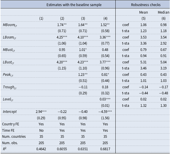
Table 2 presents the estimate for broad credit in column (1) of the baseline specification. The coefficient of determination ( $R^{2}$ ) stands at 46.42%. Hence, nearly half of the variation in forecasting performance is accounted for by time-invariant country-specific factors. The baseline model will be expanded to investigate whether forecasting performance also varies across different phases of the credit cycle.

Table 2.

Determinants of forecasting performances for forecast-augmented credit-to-GDP gaps

Variable definitions: the endogenous variable in columns (1) to (4) is the average manhattan distance between forecast-augmented credit-to-GDP gaps obtained through (recurrent) SSA forecasting and those obtained with perfect forecasts for country i during period $\tau$ . We consider 5-year periods starting in $1970q1$ to compute these average manhattan distances. Period $\tau$ =1 corresponds therefore to $1965q2-1970q1$ . Variable $ MBoom$ is the frequency of medium boom episodes (i.e., one-sided credit-to-GDP gap between 2% and 10%) during period $\tau$ ; $ LBoom$ is the frequency of large boom episodes (i.e., one-sided credit-to-GDP gap larger than 10%) during period $\tau$ . Variables $ MBust$ and $ LBust$ capture the frequency of medium and large bust episodes during period $\tau$ , respectively (defined with symmetrical thresholds, i.e., one-sided credit-to-GDP gap between −2% and −10%, and lower that −10% respectively). Variables $ Peak$ (resp. $ Trough$ ) is a dummy variable equal to 1 if a peak (resp. a trough) in the credit-to-GDP ratio is identified during period $\tau$ by the turning point algorithm proposed by Harding and Pagan (Reference Harding and Pagan2002). Variable $ Level$ is the level of the trend component of the credit-to-GDP ratio.

Note: ^***, ^** and ^* indicate significance respectively at the 1 $\%$ , 5 $\%$ and 10 $\%$ levels. Robust standard errors are in brackets. Columns (5) and (6) summarizes the results of the robustness checks, reporting mean and median respectively of coefficients and t-statistics, computed over 3840 alternative specifications (2 credit variables (broad and narrow) x 2 SSA forecasting methods (reccurent and vectorial) x 4 different horizons for generating forecast-augmented credit-to-GDP gaps (8, 12, 16, 20) x 20 different starting dates for the sample (1970q1 to 1974q4) x 6 different durations to define periods (5 to 10 years) x 2 sets of fixed effects (with or without time-fixed effects)).

The estimate reported in column (1) of Table 2 underscores the significance of country heterogeneity in forecasting performance. However, it’s important to note that this estimate is contingent on several methodological choices: the use broad credit; recurrent SSA forecasting with a forecast horizon of $k=12$ , the Manhattan distance metric, a starting date in 1970q1, and 5-year periods. Consequently, the estimated country-fixed effects might be misleading to capture country heterogeneity. To ensure the robustness of our findings, we explore a wide range of alternative specifications. Additionally, we provide descriptive statistics concerning these estimated country-fixed effects. Specifically, the alternative specifications encompass:

• • 2 credit variables: broad credit or narrow credit;

• • 2 SSA forecasting methods: recurrent or vectorial SSA forecasting;

• • 4 forecast horizons used to generate forecast-augmented credit-to-GDP gaps through SSA: $k=8,12,16$ or $20$ ;

• • 20 different starting dates: 1970q1, 1970q2,…, or 1974q4;

• • 6 durations to define periods: 5-year periods, 6-year periods,…, or 10 year periods.

These alternative specifications are instrumental in enhancing the robustness and comprehensiveness of our analysis, resulting in a total of 1920 alternative estimates.Footnote ²¹ It’s worth noting that the number of countries can vary across these alternative estimates due to data availability, particularly when the duration of periods is extended.

Table 3.

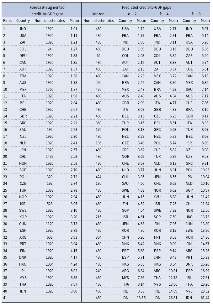
Accuracy of forecast-based credit-to-GDP gaps: country ranking

Note: The ranking of countries is based on the mean of estimated country-fixed effects computed over the full set of robustness checks (i.e., alternative estimates). The number of alternative estimates can reach 1920 for forecast-augmented credit-to-GDP gaps and 480 for predicted credit-to-GDP gaps. The number of estimates is lower for some countries due to data availability.

The results are reported in the first columns of Table 3. India, the USA and South Africa display the best performances: the Manhattan distance between forecast-augmented credit-to-GDP gaps obtained through SSA and those derived from perfect forecasts is 1.01pp, 1.11pp and 1.21pp, respectively. Additionally, the accuracy of forecast-augmented credit-to-GDP gaps produced by SSA is noticeable for Germany, Canada, Austia, France, Austalia, Mexico and Italy: the Manhattan distance averages less than 2pp in all of these countries. For these nations, forecast-augmented credit-to-GDP gaps derived from SSA provide a suitable metric for mitigating the end-of-sample problem that affect one-sided credit-to-GDP gaps. However, some countries may not find it advantageous to rely on forecast-augmented credit-to-GDP gaps. In the bottom of the ranking displayed in Table 3, Finland, Denmark, Hong Kong, Ireland, Malaysia, Thailand, Indonesia exhibit Manhattan distances averaging more than 4pp. In these countries, both one-sided credit-to-GDP gaps and forecast-augmented credit-to-GDP gaps are susceptible to significant revisions when the future path of credit-to-GDP ratios is observed.

Countries at the bottom of the ranking may have experienced large and prolonged booms and/or busts in credit-to-GDP gaps surrounding financial crises. For instance, Malaysia, Thailand, and Indonesia faced sharp credit contractions following the 1997 Asian financial crisis, while Denmark and Ireland experienced both booms and busts around the 2007–2008 Great Financial Crisis. These patterns suggest complex dynamics in credit-to-GDP gaps. Such fluctuations in the medium-term component of credit-to-GDP gaps may contribute to the poor forecasting performance observed for these countries and highlight the need for greater attention to credit market conditions.

4.1.3 Credit market conditions and forecasting performances

The augmented specification introduces time-varying covariates:

(4) \begin{eqnarray} dist_{i,\tau } &=&\beta _{1}MBoom_{i,\tau }+\beta _{2}LBoom_{i,\tau }+\beta _{3}MBust_{i,\tau }+\beta _{4}LBust_{i,\tau }+\beta _{5}Peak_{i,\tau }\nonumber \\ &&+\beta _{6}Trough_{i,\tau }+\beta _{7}Level_{i,\tau }+\delta _{\tau }+\alpha _{i}+\varepsilon _{i,\tau } \end{eqnarray}

where variable $MBoom_{i,t}$ is the frequency of medium boom episodes during period $\tau$ (defined as one-sided credit-to-GDP gap between 2% and 10%), $LBoom_{i,t}$ is the frequency of large boom episodes during period $ \tau$ (defined as one-sided credit-to-GDP gap larger than 10%).Footnote ²² Variables $MBust_{i,\tau }$ and $LBust_{i,\tau }$ capture the frequency of medium bust and large bust episodes during period $\tau ,$ respectively (defined with symmetrical thresholds, i.e., one-sided credit-to-GDP gap between −2% and −10%, and lower that −10%, respectively). Variables $ Peak_{i,\tau }$ (resp. $Trough_{i,\tau}$ ) is a dummy variable equal to 1 if a peak (resp. a trough) is identified during period $\tau$ using the turning point algorithm proposed by Harding and Pagan (Reference Harding and Pagan2002).Footnote ²³ Variable $ Level_{i,\tau }$ is the level of the trend component of the credit-to-GDP ratio and serves as an indicator of banking sector development. The augmented specification also includes controls for period-fixed effects ( $ \delta _{\tau }$ ).

Table 2 presents the estimates in columns (2) to (4), progressively incorporating covariates into the estimated specifications. We observe an increase in the coefficient of determination ( $R^{2}$ ) from 46% in column (1) to 68% in column (4), signifying the influence of credit market conditions on forecasting performance. Particularly, we find that forecasting performance experiences significant deterioration during periods of large credit booms and busts. In column (4) of Table 2, the Manhattan distance between forecast-augmented credit-to-GDP gaps obtained through SSA and those derived from perfect forecasts increases by 3.36pp and 3.77pp during large boom and bust episodes, respectively, compared to periods when the credit-to-GDP gap falls within the range of −2% to 2%. In other words, forecast-augmented credit-to-GDP gaps face challenges in mitigating the end-of-sample problem in the one-sided credit-to-GDP gap during periods of large credit booms or busts. Additionally, forecasting performance mildly deteriorates during medium credit booms, with a 1.52pp increase, but does not exhibit significant deterioration at the 10% level during medium credit busts. Table 2 also indicates that forecasting performances are only lightly mitigated during a peak in the credit-to-GDP ratio; parameter associated with variable $Peak_{i,\tau }$ is 0.81 and significant only at the 10% level. This effect is not symetrical, as the parameter associated with variable $Trough_{i,\tau }$ is not significant at the 10% level.

These results have implications for the reliability of forecast-augmented credit-to-GDP gaps in an operational context. Forecasting performances primarily declines during large boom and bust episodes, i.e., when banking supervisors already have a clear signal concerning the credit market situation. Conversely, outside of these episodes, forecast-augmented credit-to-GDP gaps continue to serve as a reliable complementary metric for banking supervisors to assess the macro-financial environment. Performance slightly deteriorates during medium credit booms and during the peak of the credit cycle, but only to a limited extent.

Furthermore, in column (4) of Table 2, we observe that forecasting performances diminishes with increased banking sector development. However, the economic significance of this effect is rather limited: a 10pp increase in trend component of the credit-to-GDP ratio results in a 0.3pp increase in the Manhattan distance ( $dist_{i,\tau}$ ).

When assessing country heterogeneity, the estimates reported in column (4) of Table 2 depends on several methodological choices: we use broad credit; recurrent SSA forecasting with a forecast horizon $k=12$ , the Manhattan distance metric, a starting date in 1970q1, and 5-year periods. Thus, we consider the same alternative specifications as those used in section 4.1.2, along with alternatives that exclude time-fixed effects from the estimated specificationsFootnote ²⁴ Consequently, we end up with a total of 3840 alternative specifications. Columns (5) and (6) of Table 2 present descriptive statistics for the estimated parameters, confirming the primary findings . It is evident that poor forecasting performances are concentrated during periods of large credit booms and busts. The Manhattan distance increases by an average of 3.53pp and 5.31pp during large boom and bust episodes, respectively, with t-statistics averaging 3.36 and 3.46, respectively, across the full set of alternative estimates. Furthermore, the robustness analysis indicates that medium credit booms and peaks in the credit-to-GDP ratio do not significantly affect forecasting performances, with t-statistics averaging 1.23 and 1.01 for coefficients associated with variables $MBoom_{i,\tau }$ and $Peak_{i,\tau }$ , respectively. Similarly, medium credit busts and troughs in the credit-to-GDP ratio do not appear to be detrimental to forecasting performances. Lastly, the robustness analysis does not provide strong evidence supporting a clear connection between banking sector development and forecasting performances. The coefficient associated with variable $Level_{i,\tau }$ averages 0.02, but t-statistic averages only 1.32.

4.2 Predicted credit-to-GDP gaps

Predicted credit-to-GDP gaps provide a forward-looking perspective in the assessment of credit market conditions. For a given period $t$ , we compare predicted credit-to-GDP gaps for horizon $k$ with one-sided credit-to-GDP gaps computed for period $t+k$ . We rely on the Manhattan distance between these two metrics to capture the accuracy of predicted credit-to-GDP gaps, for the same reasons as in the previous sub-section. In the present situation, the Manhattan distance corresponds to the mean absolute error (MAE).

4.2.1 Country heterogeneity

We assess the accuracy of predicted credit-to-GDP gaps by a cross-validation procedure. Figure 3 illustrates country heterogeneity for forecast horizons $k=1$ to $8$ , both for broad credit and narrow credit. First, Figure 3 shows that forecasting performances deteriote with forecast horizons. MAE is 4.14pp on average for forecast horizon $k=1$ and increases up to 14.33pp on average for forecast horizon $ k=8$ . Second, narrow credit displays better forecasting performances according to MAE than broad credit. However, this difference might be explain by the larger size of credit-to-GDP gaps for broad credit than for narrow credit (see Table 1). Third, Figure 3 shows that country heterogeneity is noticeable. Focusing on broad credit, the range of MAE between the 10th and the 90th percentiles is 5.10pp for forecast horizon $k=1$ and increases up to 17.73pp for forecast horizon $k=8.$ Further, countries displaying the best forecasting performances exhibit MAE around 2pp for forecast horizon $k=1,$ and up to 5pp for forecast horizon $k=8.$ We consider such average level of errors as substantial relatively to the average size of credit-to-GDP gaps (10.05pp for broad credit for instance, see Table 1).Footnote ²⁵

Figure 3.

Predicted credit-to-GDP gaps.

Note: The top 5 with the lowest MAE is: 1.USA, 2.BRA, 3.ZAF, 4.FRA, 5.COL. The top 5 for largest MAE is: 1.IRL, 2.ARG, 3.MYS, 4.THA, 5.ESP. Top 5 are based on the average ranking of each country over the 8 forecast horizons. Note: The top 5 with the lowest MAE is: 1.IND, 2.ARG, 3.ZAF, 4.USA, 5.FRA. The top 5 for largest MAE is: 1.IDN, 2.MYS, 3.THA, 4.HKG, 5.ESP. Top 5 are based on the average ranking of each country over the 8 forecast horizons.

4.2.2 Country ranking

We rely on the same baseline regression model as in section 4.1.2 to assess more cautiously country heterogeneity:

(5) \begin{equation} dist_{i,\tau }^{k}=\alpha _{i}+\varepsilon _{i,\tau } \end{equation}

where $dist_{i,\tau }^{k}$ is the MAE of predicted credit-to-GDP gaps at horizon $k$ for country $i$ during period $\tau$ . We consider 5-year periods in the baseline estimate starting in 1970q1. Table 4 reports estimates for broad credit of the baseline specification in columns (1), (3), (5) for forecast horizons $k=2,4,8$ respectively.Footnote ²⁶ $R^{2}$ is 35.41% for forecast horizon $k=2$ and decreases to 28.90% for forecast horizon $k=8$ . 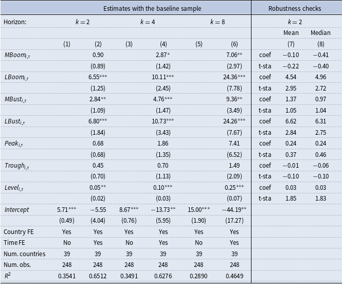Therefore, time-invariant country-specific factors have a substantial importance but do not explain the main part of dispersion in forecasting performances. In addition, time-invariant factors become less important when forecast horizon increases.

Table 4.

Determinants of forecasting performances for predicted credit-to-GDP gaps

Variable definitions: the endogenous variable is the MAE of predicted credit-to-GDP gaps obtained by (recurrent) SSA at horizons k = 2, 4, 6 or 8 for country i during period $\tau$ . We consider 5-year periods to compute MAE in the baseline estimate starting in 1970q1. Period $\tau$ =1 corresponds therefore to 1965q2–1970q1. Variable $ MBoom$ is the frequency of medium boom episodes during period t (defined as one-sided credit-to-GDP gap between 2% and 10%); $ LBoom$ is the frequency of large boom episodes during period t (defined as one-sided credit-to-GDP gap larger than 10%). Variables $ MBust$ and $ LBust$ capture the frequency of medium bust and large bust episodes during period t respectively (defined with symmetrical thresholds, i.e., one-sided credit-to-GDP gap between −2% and −10%, and lower that −10% respectively). Variables $ Peak$ (resp. $ Trough$ ) is a dummy variable equal to 1 if a peak (resp. a trough) is identified during period t by the turning point algorithm proposed by Harding and Pagan (Reference Harding and Pagan2002). Variable $ Level$ is the level of the trend component of the credit-to-GDP ratio.

Note: ^***, ^** and ^* indicate significance respectively at the 1 $\%$ , 5 $\%$ and 10 $\%$ levels. Robust standard errors are in brackets. Columns (7) and (8) summarizes the results of the robustness checks, reporting mean and median repectively of coefficients and t-statistics, computed over 960 alternative specifications (2 credit variables (broad and narrow) x 2 SSA forecasting methods (reccurent and vectorial) x 20 different starting dates for the sample (1970q1 to 1974q4) x 6 different durations to define periods (5 to 10 years) x 2 sets of fixed effects (with or without time-fixed effects)). Robustness checks concern only forecast horizon k = 2 to save space.

We consider the same kind of robustness exercice as in section 4.1.2 to get a more cautious assessment of forecasting performances at the country level. For each forecast horizon, we have 480 alternative estimates of the baseline specification.Footnote ²⁷ Results are reported in the last columns of Table 3 only for forecast horizons $ k=2,4$ and $8$ to save space. More precisely, Table 3 reports for forecast horizon $k=2$ : country ranking, the number of estimates per country, and the mean of estimated country-fixed effects. We notice first that the USA, France, India and Germany display the best performances with MAE lower than 2pp on average. Table 3 shows that country ranking does not depend much on forecast horizon. The USA, France, India and Germany always remain in the top 4 for instance. Second, countries in the bottom of the ranking are Malaysia, Thailand, Ireland and Indonesia, whatever the forecast horizon. MAE is already larger than 7pp at forecast horizon $k=2$ in these countries. Third, Table 3 suggests that the reliability of predicted credit-to-GDP gaps and forecast-augmented credit-to-GDP gaps are not independent. The top and bottom of the rankings are quite similar in Table 3. Austria, South Africa, Canada, Mexico and Austalia are also always well ranked. Last, Table 3 confirms that forecasting performances substantially deteriorate with forecast horizon. MAE is larger than 5pp on average for forecast horizons $ k=8$ in top ranked countries for instance; indicating that MAE is multiplied by more that 2.5 from forecast horizon $k=2$ to $k=8$ .

5.1 Prediction of credit booms

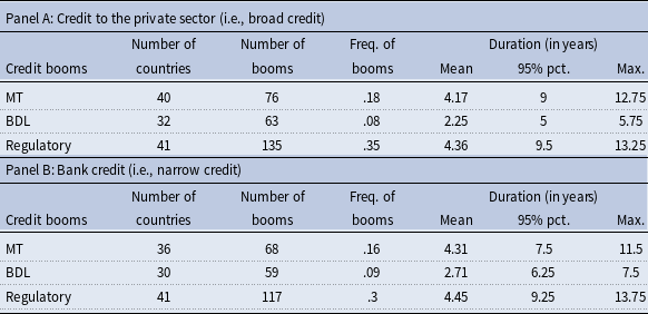
We adopt the definitions proposed by Barajas et al. (Reference Barajas, Dell’Ariccia and Levchenko2007) and Mendoza and Terrones (Reference Mendoza and Terrones2008) to identify credit booms (henceforth BDL and MT, respectively).Footnote ²⁹ Further, we also rely on a “regulatory” definition of credit booms: credit booms are associated with periods with credit gaps higher than 2%. This aligns with the criteria where the CCyB might be activated, as specified in the BCBS guidelines (BCBS (2010)).Footnote ³⁰ We employ these three alternative definitions of credit booms in our analysis to ensure robustness. Table 5 presents descriptive statistics on credit booms, with all three credit boom definitions applied using two-sided credit-to-GDP gaps for both broad credit (Panel A) and narrow credit (Panel B). The MT and BDL definitions yield a relatively similar number of credit booms (76 and 63, respectively, for broad credit, for example). The primary difference lies in the duration of credit booms, with MT averaging 4.17 years, while BDL averages 2.25 years for broad credit, for instance. This implies that, according to the MT and BDL definitions, countries experience credit booms for approximately 18% and 8% of the time, respectively. In contrast, the regulatory definition of credit booms results in a more lenient identification of such periods. We identify 135 credit booms for broad credit, with an average duration of 4.36 years, signifying that countries experience credit booms for approximately 35% of the time.

Table 5.

Identification of credit booms

Note : Credit-to-GDP gaps are computed by two-sided SSA. We rely first on Mendoza and Terrones (Reference Mendoza and Terrones2008) and Barajas et al. (Reference Barajas, Dell’Ariccia and Levchenko2007) to identify credit booms, called MT and BDL credit booms respectively. In addition, we define regulatory credit booms as periods with credit-to-GDP gaps higher than 2% during at least 4 consecutive quarters. We consider 41 countries (Luxembourg and Russia are excluded from the initial sample of 43 countries due to limited data availability) with samples ending in 2019q4. The number of countries reported in the table corresponds to countries (over 41) that experienced at least one credit boom. Freq. of booms is the proportion of time countries spend in credit booms.

We shift our focus to a more specific event: the probability of entering a credit boom. We employ a pooled logit model as the link function:

(6) \begin{equation} P(CB_{i,t}^{ts}=1)=\frac {1}{1+\exp \left [ -\alpha -\beta CY_{i,t}^{os}-\gamma FBCY_{i,t}^{os}\right ] }, \end{equation}

where the subscripts refer to country $i$ in period $t$ . The variable $ CB_{i,t}^{ts}$ is a binary variable that is equal to 1 if a credit boom identified with two-sided credit-to-GDP gap occurs and 0 otherwise, $ CY_{i,t}^{os}$ is the one-sided credit-to-GDP gap, $FBCY_{i,t}^{os}$ is an indicator (or a set of indicators) derived from forecast-based credit-to-GDP gaps.Footnote ³¹ Parameters $\alpha$ , $\beta$ and $\gamma$ are estimated by maximum likelihood, with standard errors computed via the clustered version (at the country level) of the Huber-White estimator for robustness against heteroscedasticity. Further, credit booms often extend over multiple quarters, constituting multiquarter events. However, the pooled logit model assumes independence between observations. To address this, we apply a common data treatment by retaining only the initial period of these multiperiod events. This allows us to consider observations as independent from each other.

We consider two categories of indicators derived from forecast-based credit-to-GDP gaps to represent the variable $FBCY_{i,t}^{os}$ . Firstly, we examine difference between the one-sided credit-to-GDP gap and the forecast-augmented credit-to-GDP gap ( ${ CY}_{i,t}^{os}{ -CY} _{i,t}^{RFA12}$ ). The end-of-sample problem associated with the one-sided credit-to-GDP gap implies that rapid increases in credit activities in the near future are not anticipated. As a result, these increases are not factored into the assessment of the trend-cycle decomposition. Consequently, the current trend in credit-to-GDP ratio may be underestimated, with a significant portion of the credit expansion allocated to the cyclical component. This effect may become particularly pronounced when the trend dynamics are exceptionally smooth. The forecast-augmented credit-to-GDP gap is designed to address this end-of-sample problem. Consequently, during credit boom periods, one-sided credit-to-GDP gap and forecast-augmented credit-to-GDP gap may diverge, with the one-sided credit-to-GDP gap potentially exceeding the forecast-augmented credit-to-GDP gap during the initial phase of a credit boom.Footnote ³²

Secondly, we consider the difference between the predicted credit-to-GDP gap at horizon 4 and the one-sided credit-to-GDP gap ( ${ CY}_{i,t}^{RFor4} { -CY}_{i,t}^{os}$ ). The primary purpose of this variable is to ascertain whether larger imbalances are expected in the forthcoming periods. Positive differences signify an anticipation of cyclical credit activities expanding over the next year. This information can be valuable for predicting the onset of a credit boom episode in the economy.

Table 6.

Prediction of credit booms

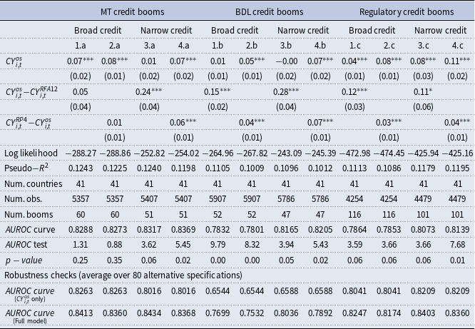
Variable definitions: ${ CY}^{{ os}}$ : credit-to-GDP gap obtained through one-sided SSA; ${ CY}^{{ RFA12}}$ : forecast-augmented credit-to-GDP gap (with forecasts extending by 12 periods); ${ CY}^{{ RP4}}$ : predicted credit-to-GDP gap at horizon 4. These forecast-based credit-to-GDP gaps are derived using recurrent SSA forecasting.

Note : ^***, ^** and ^* indicate significance respectively at the 1 $\%$ , 5 $\%$ and 10 $\%$ levels. Robust standard errors are in brackets. We calculate credit-to-GDP gaps using SSA. Credit booms are identified using two-sided credit-to-GDP gaps. Specifically, MT and BDL refer to credit booms identified with definitions based on Mendoza and Terrones (Reference Mendoza and Terrones2008) and Barajas et al. (Reference Barajas, Dell’Ariccia and Levchenko2007), respectively. We define regulatory credit booms as periods where credit-to-GDP gaps remain above 2% for at least four consecutive quarters. We consider an unbalanced sample ending in 2019q4 for the baseline analysis. The bottom lines in the table summarize the results of the robustness checks, reporting the average AUROC curve computed over 80 alternative specifications when the model only includes the one-sided credit-to-GDP gap and when forecast-based credit-to-GDP gaps are also added. The alternative specifications encompass 2 filters (SSA and HP) x 2 forecasting methods (reccurent and vectorial) x 4 forecast horizons for generating forecast-based credit-to-GDP gaps x 5 different end dates (q4 of 2015 to 2019) for the sample.

The estimates are presented in Table 6.Footnote ³³ The predictive power of the model is assessed by the AUROC curve. For broad credit, the AUROC curve values are around 0.82 for MT credit booms and 0.78 for BDL and regulatory credit booms. These results suggest that the predictive power of one-sided credit gaps can be considered excellent for MT credit booms and acceptable for BDL and regulatory credit booms. Additionally, the forecast-augmented credit-to-GDP gap, especially its difference with the one-sided credit-to-GDP gap, provides valuable information for predicting credit booms. The coefficient associated with the variable ( ${ CY} _{i,t}^{os}{ -CY}_{i,t}^{RFA12}$ ) is significant at the 1% or 10% level in the estimated models reported in Tables 6, except when both broad credit and MT credit booms are considered. Furthermore, the AUROC test (DeLong et al. (Reference DeLong, DeLong and Clarke-Pearson1988)) shows that including the variable ( ${ CY}_{i,t}^{os}{ -CY}_{i,t}^{RFA12}$ ) in the model can significantly enhance the AUROC curve.

Predicted credit-to-GDP gaps also offer valuable information for predicting credit booms. The coefficient associated with the variable ( ${ CY} _{i,t}^{RFor4}{ -CY}_{i,t}^{os}$ ) is significant at the 1% level in most estimated specifications in Table 6, with the exception of when both broad credit and MT credit booms are considered. In addition, the AUROC test shows that including the variable ( ${ CY}_{i,t}^{RFor4} { -CY}_{i,t}^{os}$ ) can significantly improve the predictive power of the model. The difference between the predicted credit-to-GDP gap at horizon 8 and the predicted credit-to-GDP gap at horizon 4 ( ${ CY} _{i,t}^{RFor8}{ -CY}_{i,t}^{RFor4}$ ) has also been added for robustness checks to include a second indicator based on predicted credit-to-GDP gaps. However, the additional information provided by this variable was rarely significant at the 10% level. Therefore, a single indicator based on predicted credit-to-GDP gaps performs well in accounting for future expected expansions in credit market imbalances.

5.2 Robustness checks

We investigate the robustness of these results by considering a large set of alternative specifications. In baseline estimates of equation (6) reported in Table 6, we rely on SSA to derive the variable $CY_{i,t}^{os}$ , and we rely on recurrent SSA forecasting to generate the $FBCY_{i,t}^{os}$ indicators. In addition, forecast-augmented credit-to-GDP gaps are derived from series extended by 12 periods; and we focus on predicted credit gaps at horizon 4. Last, the sample ends in 2019q4 in our baseline estimates. However, two-sided credit-to-GDP gaps are also exposed to the end-of-sample problem. Thus, some of the later periods may be excluded to mitigate this problem.

For our robustness checks, we explore two distinct filters for generating the variable $CY_{i,t}^{os}$ (SSA and HP), two forecasting methods (reccurent and vectorial) to compute the $FBCY_{i,t}^{os}$ indicators, 4 different horizons for generating forecast-augmented credit-to-GDP gaps (8, 12, 16, 20), 4 different horizons for predicted credit-to-GDP gaps (2, 4, 6, 8), and 5 different end dates (q4 of 2015 to 2019). As a result, we encompass a total of 80 alternative specifications for forecast-augmented credit-to-GDP gaps and an additional 80 alternative specifications for predicted credit-to-GDP gaps. These comprehensive robustness checks are conducted for the two credit agregate (broad and narrow) and the 3 credit boom definitions (MT, BDL and regulatory). At the bottom of Table 6, we report the average AUROC curve when the model only includes the one-sided credit-to-GDP gap and when forecast-based credit-to-GDP gaps are also added. These robustness checks validate our key findings, demonstrating that forecast-augmented credit-to-GDP gaps and predicted credit-to-GDP gaps consistently provide supplementary valuable information for detecting credit booms.Footnote ³⁴ The average AUROC curve consistently increases when indicators computed from forecast-based credit-to-GDP gaps are incorporated into our estimated specifications.

5.3 Illustration

Figure 4 illustrates the behavior of the one-sided credit-to-GDP gap (Figure 4-a) and indicators derived from forecast-based credit-to-GDP gaps (Figure 4-b & c) in the periods leading up to a credit boom. To model the behavior of these variables, we employ restricted cubic spline functions.Footnote ³⁵ We focus on BDL credit booms and broad credit in Figure 4 to save space. Figure 4-a illustrates why the one-sided credit-to-GDP gap serves as a reliable predictor of credit booms. This metric starts to exhibit notable growth well in advance of the credit boom’s commencement, surging to over 3% in the year preceding the credit boom. As demonstrated in Table 6, the difference between the one-sided credit-to-GDP gap and the forecast-augmented credit-to-GDP gap offers valuable additional insights into predicting a credit boom. Figure 4-b highlights that this indicator gradually increases several years prior to a credit boom, eventually surpassing a 2-percentage-point threshold. In other words, the one-sided credit-to-GDP gap overshoots the forecast-augmented credit-to-GDP gap by more than 2 percentage points before a credit boom. The difference between the predicted credit-to-GDP gap at horizon 4 and the one-sided credit-to-GDP gap (Figure 4-c) exhibits a more pronounced change before a credit boom. The predicted credit-to-GDP gap at horizon 4 experiences rapid growth and becomes 4 percentage points higher than the one-sided credit-to-GDP gap prior to a credit boom. Consequently, the predicted credit-to-GDP gap captures the fact that credit activities are set to continue expanding rapidly, with the peak yet to come.

Figure 4.

Behavior of credit-to-GDP gaps before a credit boom.

Note: the gray area corresponds to the one-standard error band.

From a macro-prudential standpoint, Figure 4 suggests that banking supervisors should rely on both the forecast-augmented credit-to-GDP gap and the predicted credit-to-GDP gap to identify shifts in the macro-financial environment. The risk of a credit boom becomes evident when the one-sided credit-to-GDP gap exceeds 3%. This signal becomes notably more reliable if the one-sided credit-to-GDP gap overshoots the forecast-augmented credit-to-GDP gap by more than 2 percentage points, and if the predicted credit-to-GDP gap indicates that the credit-to-GDP gap will increase by more than 4 percentage points in the upcoming year.