1. Introduction
Shallow-flow modelling usually eliminates one or two spatial dimensions by considering average properties over the depth of a thin fluid layer. This modelling approach is current in hydraulics (Chow Reference Chow1959), dealing with turbulent open-channel flows. In this context, backwater curves denote 1D steady depth profiles
 $h(x)$
and obey the backwater equation
 $(1-Fr)h^{\prime }=I-J$
where
 $Fr$
is a Froude number,
 $I$
is the bottom slope and
 $J$
is the lineic head loss due to bottom friction. When
 $I>0$
is constant, the relative values of the critical height
 $h_{c}$
, such that
 $Fr=1$
, and the normal height
 $h_{n}$
, such that
 $I=J$
, lead to three
 $M$
-curve types in the weak slope regime
 $h_{c}<h_{n}$
and to three
 $S$
-curve types in the strong slope regime
 $h_{n}<h_{c}$
. When
 $I(x)$
varies with space, transitions between the fluvial (
 $Fr<1$
) and the torrential (
 $Fr>1$
) regimes can occur through hydraulic jumps or transcritical transition (e.g. Bukreev, Gusev & Lyapidevskii Reference Bukreev, Gusev and Lyapidevskii2002 or Zerihun & Fenton Reference Zerihun and Fenton2006). These backwater curves can be viewed as steady solutions of the Saint-Venant equations (de Saint-Venant Reference de Saint-Venant1871), also called the shallow-water equations.
The laminar flows of thin viscous liquid layers are also modelled by shallow-flow equations. Benney (Reference Benney1966) and Shkadov (Reference Shkadov1967) derived such models by retaining only a parabolic velocity profile in a Galerkin approximation of the 2D vertical Navier–Stokes equations and justified it by the good agreement with the experiments of Kapitsa & Kapitsa (Reference Kapitsa and Kapitsa1949). Numerous subsequent works have proposed asymptotic expansion leading to a 1D partial differential equation for the depth
 $h(x,t)$
and the lineic discharge flux
 $q(x,t)$
, often taking into account the effect of surface tension and considering various bottom slopes (Lin Reference Lin1969; Gjevik Reference Gjevik1970; Nakaya Reference Nakaya1975; Pumir, Manneville & Pomeau Reference Pumir, Manneville and Pomeau1983; Alekseenko, Nakoryakov & Pokusaev Reference Alekseenko, Nakoryakov and Pokusaev1985; Roberts Reference Roberts1996; Oron, Davis & Bankoff Reference Oron, Davis and Bankoff1997; Ruyer-Quil & Manneville Reference Ruyer-Quil and Manneville1998, Reference Ruyer-Quil and Manneville2000, Reference Ruyer-Quil and Manneville2005; Nguyen & Balakotaiah Reference Nguyen and Balakotaiah2000; Shkadov & Sisoev Reference Shkadov and Sisoev2004; Boutounet et al.
Reference Boutounet, Chupin, Noble and Vila2008; Sadiq & Usha Reference Sadiq and Usha2008; Fernàndez-Nieto, Noble & Vila Reference Fernàndez-Nieto, Noble and Vila2010; Samanta, Ruyer-Quil & Goyeau Reference Samanta, Ruyer-Quil and Goyeau2011; Noble & Vila Reference Noble and Vila2013; Chakraborty et al.
Reference Chakraborty, Nguyen, Ruyer-Quil and Bontozoglou2014,
 $\ldots$
). Starting with the so-called ‘boundary-layer equation’, similar to Prandtl’s equations (Schlichting Reference Schlichting1955), the difficulty of these modelling approaches lies in the information required about the velocity profile in the integration direction. Most works suggest fixed shapes such as the parabolic one in the laminar cases. More elaborate approaches, such as the weighted-residual method of Ruyer-Quil & Manneville (Reference Ruyer-Quil and Manneville1998), are based on well suited Galerkin approximation functions that minimize the number of resulting equations. Following a different approach, we present an approximation method that leads to a single backwater equation associated with similarity solutions for the velocity profiles.
Here, we consider laminar flows of Newtonian fluids with negligible surface tension effects in the presence of a small and slowly varying bottom slope such that the product
 ${\it\Gamma}=Re\,I$
of the slope
 $I$
and the Reynolds number
 $Re$
is of order one, while
 $I$
is small. For instance, the case
 $I=0.01$
and
 $Re=100$
satisfies this requirement while ensuring that the flow is laminar. As for most asymptotic expansions, this choice aims to balance a maximum of terms in the equations, that is, for the present case, acceleration, pressure, bottom slope and friction in the momentum equations.
Under this asymptotic expansion, we express the steady solution velocities in the form
 $u=T/h$
and
 $v=L(\text{d}h/\text{d}X)/h-\partial M/\partial X$
where
 $T$
,
 $L$
and
 $M$
are functions of
 $X=x/Re$
and
 $Y=y/h$
, being related through
 $L=YT$
and
 $\partial M/\partial Y=T$
. This leads to the ‘TLM model’ in which the
 $X$
dependency of the
 $T$
profiles is contained in the term
 $h[(\partial M/\partial X)(\partial T/\partial Y)-(\partial T/\partial X)T]$
that appears to be often small compared to the others. When it is so, the steady flow is described by the similarity model in which
 $T$
and
 $L$
no longer depend on
 $X$
(STL model). Such a similarity assumption for the velocity profiles was introduced by Serre (Reference Serre1953), but the shape of the velocity profiles had to be imposed eventually. Instead of using a Galerkin approximation and averaging over the vertical, as is often done in the literature, our TLM and STL models involve an implicit relation for
 $h$
and
 $\text{d}h/\text{d}X$
through a nonlinear 1D eigenvalue problem, as explained in § 2. These models are then compared to each other in § 3 in the case of transcritical flows.
2. Three shallow-water steady models
2.1. The TLM shallow-water model
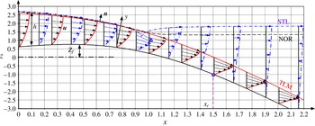
We consider an infinitely wide channel whose bottom is defined by the equation
 $z=Z_{f}(x)$
where
 $(x,z)$
are respectively the horizontal and vertical coordinates in the presence of gravity
 $g$
(figure 1). If
 $y$
denotes the coordinate perpendicular to the bottom at some location, we suppose that the slope
 $I=-Z_{f}^{\prime }(x)$
is small enough to consider that
 $x$
is also the coordinate in the direction tangential to the bottom. Within this approximation and denoting by
 ${\it\varphi}_{x}$
the derivatives
 $(\partial {\it\varphi}/\partial x)(x,y)$
or
 ${\it\varphi}^{\prime }(x)$
of a quantity
 ${\it\varphi}$
, the steady 2D incompressible Navier–Stokes equations read
 $$\begin{eqnarray}\displaystyle \left.\begin{array}{@{}ll@{}}\widetilde{u}_{x}+\widetilde{v}_{y}=0, & \widetilde{u}\widetilde{u}_{x}+\widetilde{v}\widetilde{u}_{y}=-\widetilde{p}_{x}+I+Re^{-1}(\widetilde{u}_{xx}+\widetilde{u}_{yy}),\\ & \widetilde{u}\widetilde{v}_{x}+\widetilde{v}\widetilde{v}_{y}=-\widetilde{p}_{y}-1+Re^{-1}(\widetilde{v}_{xx}+\widetilde{v}_{yy}),\end{array}\right\} & & \displaystyle\end{eqnarray}$$
where the velocities
 $\widetilde{u}$
and
 $\widetilde{v}$
are made non-dimensional by
 $q^{1/3}g^{1/3}$
and all spatial coordinates by
 $q^{2/3}g^{-1/3}$
, with
 $q$
denoting the constant lineic discharge flux. The Reynolds number is
 $Re=q/{\it\nu}$
where
 ${\it\nu}$
is the kinematic viscosity.
2D flow
 $\boldsymbol{u}$
of a layer of depth
 $h$
over a slowly variable bottom
 $z=Z_{f}(x)$
. Comparison of three shallow-water steady models for a transcritical flow: TLM in plain red, STL in dash-dotted blue and NOR in dashed black. The TLM backwater curve is critical at
 $x=x_{c}$
.

The boundary conditions at the bottom, defined by the equation
 $y=0$
, are
 $\widetilde{u}=\widetilde{v}=0$
. On the free surface, defined by the equation
 $y=\widetilde{h}(x)$
, the kinematic and dynamic boundary conditions are respectively
 $\widetilde{u}\widetilde{h}_{x}=\widetilde{v}$
and
 $(\widetilde{p}-\widetilde{p}_{a})\boldsymbol{n}=2Re^{-1}\widetilde{\unicode[STIX]{x1D659}}\boldsymbol{\cdot }\boldsymbol{n}$
where
 $p_{a}$
is the constant atmospheric pressure,
 $\boldsymbol{n}$
is the normal to the free surface and
 $\widetilde{\unicode[STIX]{x1D659}}$
is the strain rate tensor.
Since the slope
 $I$
is small, we consider the following asymptotic expansion with
 ${\it\epsilon}\ll 1$
:
 $$\begin{eqnarray}\displaystyle \left.\begin{array}{@{}c@{}}{\it\epsilon}=Re^{-1},\quad {\it\Gamma}=Re\,I,\quad \widetilde{h}=h({\it\epsilon}x)+O({\it\epsilon}),\\ \widetilde{u}=u({\it\epsilon}x,y)+O({\it\epsilon}),\quad \widetilde{v}={\it\epsilon}v({\it\epsilon}x,y)+O({\it\epsilon}^{2}),\quad \widetilde{p}=p({\it\epsilon}x,y)+O({\it\epsilon}),\end{array}\right\} & & \displaystyle\end{eqnarray}$$
where
 ${\it\Gamma}$
,
 $h$
,
 $v$
and
 $p$
are of order one. Since
 $I=O({\it\epsilon})$
, the coordinate
 $x$
can be considered to refer to the direction tangential to the bottom. We denote by
 $X={\it\epsilon}x$
the slow streamwise coordinate. At the leading order of the expansion, one gets the following system for
 $u(X,y)$
,
 $v(X,y)$
and
 $h(X)$
:
 $$\begin{eqnarray}u_{X}+v_{y}=0,\quad uu_{X}+vu_{y}=-h_{X}+{\it\Gamma}+u_{yy},\end{eqnarray}$$
with
 $u(X,0)=v(X,0)=0$
,
 $u(X,h)h_{X}=v(X,h)$
and
 $u_{y}(X,h)=0$
for the boundary conditions, with
 $\int _{0}^{h}u(X,y)\,\text{d}y=1$
as a constraint to express the constant dimensionless discharge flux. Note that the pressure
 $p$
is hydrostatic in the framework of this analysis.
We look at solutions of (2.3a,b ) with the general form
 $$\begin{eqnarray}u(X,y)=\frac{1}{h(X)}T\left(X,\frac{y}{h(X)}\right),\end{eqnarray}$$
which leads to the ‘TLM model’ for
 $T(X,Y)$
and
 $h(X)$
:
 $$\begin{eqnarray}0=T_{YY}+h^{3}({\it\Gamma}-h_{X})+h_{X}T^{2}+h(M_{X}T_{Y}-T_{X}T),\end{eqnarray}$$
where
 $M(X,Y)=\int _{0}^{Y}T(X,Z)\,\text{d}Z$
, with
 $T(X,0)=T_{Y}(X,1)=0$
and
 $M(X,1)=1$
. The vertical velocity reads
 $v=(h_{X}/h)L(X,y/h)-M_{X}$
with
 $L(X,Y)=YT(X,Y)$
.
This equation with its three constraints determines one unknown scalar. If we impose a bathymetry
 $Z_{f}(X)$
of slope
 ${\it\Gamma}(X)=-Z_{f}^{\prime }(X)$
, we can compute
 $h^{\prime }(X)={\it\Sigma}$
where
 ${\it\Sigma}$
is the solution of (2.5) and then integrate to obtain the backwater curve
 $h(X)$
.
2.2. The one-parameter family profiles of the STL model
We denote by ‘STL’ the model obtained by ignoring the
 $h$
term (
 $M_{X}T_{Y}-T_{X}T$
) in the TLM model. Similarity solutions
 $u(X,y)=T[y/h(X)]/h(X)$
are thus described by this STL model. Denoting
 ${\it\Delta}=h^{3}({\it\Gamma}-{\it\Sigma})$
, this model reduces to the ordinary differential equation
 $0=T^{\prime \prime }+{\it\Delta}+{\it\Sigma}T^{2}$
, subject to the three constraints
 $T(0)=T^{\prime }(1)=0$
and
 $\int _{0}^{1}T(Y)\,\text{d}Y=1$
. We use a finite difference scheme
 $(N\!-\!1)^{2}(T_{n+1}-2T_{n}+T_{n-1})$
for
 $n=2,\ldots ,N\!-\!1$
to approximate
 $T^{\prime \prime }$
, where the
 $T_{n}$
values are the values of
 $T$
at
 $N$
equally distributed points in the interval
 $Y\in [0,1]$
. The three constraints of (2.5) read
 $T_{1}=T_{N}-T_{N\!-\!1}=0$
and
 $\sum _{1}^{N}T_{n}=N$
. The function fsolve of Scilab (Scilab Enterprises 2012) is used with
 ${\it\Sigma}$
considered as a control parameter to determine a branch of solutions
 ${\it\Sigma}=\mathscr{S}({\it\Delta})$
. We have checked that the resolution
 $N=101$
provided sufficient accuracy for most of the cases presented here.
Part of the branch of solutions
 ${\it\Sigma}=\mathscr{S}({\it\Delta})$
passing through the linear case
 $({\it\Sigma},{\it\Delta})=(0,3)$
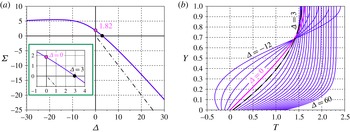
is displayed in figure 2. The corresponding velocity profiles
 $T_{{\it\Delta}}(Y)$
range from a shear profile for
 ${\it\Delta}=-\infty$
up to a plug-like profile (
 $T_{\infty }=1$
with a boundary layer at
 $Y=0$
) for
 ${\it\Delta}=\infty$
, passing through the parabolic profile
 $T_{3}(Y)=(3/2)Y(2-Y)$
for the linear case.
(a) Branch of solutions
 ${\it\Sigma}=\mathscr{S}({\it\Delta})$
for
 ${\it\Delta}\in [-30,30]$
and (b) corresponding profiles
 $T_{{\it\Delta}}(Y)+{\it\Delta}/50$
(the shift is for clarity) for
 ${\it\Delta}\in [-12,60]$
. The special value
 $\mathscr{S}(0)\sim 1.82$
is shown in magenta.

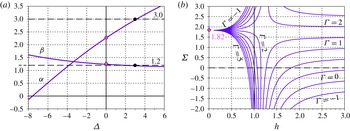
(a) Plot of
 ${\it\alpha}({\it\Delta})$
and
 ${\it\beta}({\it\Delta})$
. (b) Slope
 ${\it\Sigma}=h_{X}$
as a function of
 $h$
for
 ${\it\Gamma}\in [-1,5]$
.

In order to obtain a synthetic overview of our STL model, we integrate the equation
 $0=T^{\prime \prime }+{\it\Delta}+{\it\Sigma}T^{2}$
over the interval
 $Y\in [0,1]$
to obtain
 $$\begin{eqnarray}[h^{3}-{\it\beta}({\it\Delta})]h^{\prime }(X)=h^{3}{\it\Gamma}(X)-{\it\alpha}({\it\Delta})\quad \text{with }{\it\Delta}=h^{3}[{\it\Gamma}(X)-h^{\prime }(X)],\end{eqnarray}$$
where
 ${\it\alpha}({\it\Delta})=T_{{\it\Delta}}^{\prime }(0)$
and
 ${\it\beta}({\it\Delta})=\int _{0}^{1}T_{{\it\Delta}}^{2}(Y)\,\text{d}Y$
are plotted in figure 3(a). When the velocity profile
 $T_{{\it\Delta}}$
is the parabolic solution
 $T_{3}$
, one recovers the values
 ${\it\alpha}(3)=3$
and
 ${\it\beta}(3)=1.2$
that are commonly used for laminar shallow flows. The solutions
 ${\it\Sigma}=h^{\prime }(X)$
of the implicit (2.6) are displayed in figure 3(b) as functions of
 $h$
for various values of
 ${\it\Gamma}$
. For
 ${\it\Gamma}\in [1.82,3]$
, the resulting backwater curves exhibit more complex topologies than the usual one obtained with constant values of
 ${\it\alpha}$
and
 ${\it\beta}$
.
2.3. Determination of the transcritical point with the NOR and STL models
We denote by NOR the model for which
 ${\it\alpha}=3$
and
 ${\it\beta}=1.2$
are kept constant, as if the velocity profiles were stuck to the parabola of the normal flow that would be obtained for
 $h=h_{n}=(3/{\it\Gamma})^{1/3}$
. The backwater curves are thus solutions of the ordinary differential equation
 $h^{\prime }(X)=[h^{3}{\it\Gamma}(X)-3](h^{3}-1.2)^{-1}$
. The general solutions of the NOR model can be sought by considering the family of trajectories
 $[X(s),h(s)]$
that are solutions of the system
 ${\dot{X}}=D(h)$
and
 ${\dot{h}}=N(X,h)$
with
 $D(h)=h^{3}-1.2$
and
 $N(X,h)=h^{3}{\it\Gamma}(X)-3$
. The critical point
 $(X_{c},h_{c})$
, forming a saddle node for the phase portrait of the dynamical system, is obtained for
 $D(h_{c})=N(X_{c},h_{c})=0$
, leading to
 $h_{c}=1.2^{1/3}$
and
 ${\it\Gamma}_{c}(X_{c})={\it\Gamma}_{c}=2.5$
. The linearization of the dynamical system around the critical point leads to the matrix
 $\unicode[STIX]{x1D63C}$
with the components
 $\unicode[STIX]{x1D608}_{11}=0$
,
 $\unicode[STIX]{x1D608}_{12}=D^{\prime }(h_{c})=3h_{c}^{2}$
,
 $\unicode[STIX]{x1D608}_{21}=h_{c}^{3}{\it\xi}$
and
 $\unicode[STIX]{x1D608}_{22}=3h_{c}^{2}{\it\Gamma}_{c}$
where
 ${\it\xi}={\it\Gamma}^{\prime }(X_{c})$
measures the curvature of the bottom at the critical point. The ‘eigenslopes’ of
 $\unicode[STIX]{x1D63C}$
, that is the slope of its eigenvectors, read
 $$\begin{eqnarray}{\it\Sigma}_{\pm }({\it\xi})=\frac{{\it\Gamma}_{c}}{2}\left(1\pm \sqrt{1+\frac{4{\it\xi}h_{c}}{3{\it\Gamma}_{c}^{2}}}\right).\end{eqnarray}$$
It appears that this expression is also valid for the STL model (2.6) with
 $h_{c}=1$
and
 ${\it\Gamma}_{c}=3$
. To prove it, we consider, as for the NOR model, the following dynamical system:
 $$\begin{eqnarray}\displaystyle \left.\begin{array}{@{}c@{}}{\dot{X}}=D[X,h,{\dot{h}}/{\dot{X}}]\quad \text{with }D(X,h,{\it\Sigma})=h^{3}-{\it\beta}(h^{3}[{\it\Gamma}(X)-{\it\Sigma}]),\\ {\dot{h}}=N[X,h,{\dot{h}}/{\dot{X}}]\quad \text{with }N(X,h,{\it\Sigma})=h^{3}{\it\Gamma}(X)-{\it\alpha}(h^{3}[{\it\Gamma}(X)-{\it\Sigma}]).\end{array}\right\} & & \displaystyle\end{eqnarray}$$
At first, the critical point is at the intersection of the lines
 ${\dot{h}}=0$
and
 ${\dot{X}}=0$
in the
 $(X,h)$
plane. The first condition reads
 ${\it\Delta}={\it\alpha}({\it\Delta})$
, leading to
 ${\it\Delta}=3$
and
 $h=h_{n}(X)=[3/{\it\Gamma}(X)]^{1/3}$
. It describes the lines of the normal heights as
 ${\it\Sigma}=0$
. The second condition can be satisfied only when
 $h^{\prime }(X)\rightarrow -\infty$
and leads to
 $h=1$
since it can be numerically checked that
 $(1-{\it\beta})/{\it\alpha}\rightarrow 0$
when
 ${\it\Delta}\rightarrow +\infty$
. As announced, we find
 $h_{c}=1$
and
 ${\it\Gamma}(X_{c})=3$
when both conditions are met.
We now determine whether a straight line trajectory with the equation
 $X_{{\it\Sigma}}(s)=X_{c}+{\it\eta}(s)$
and
 $h_{{\it\Sigma}}(s)=h_{c}+{\it\Sigma}{\it\eta}(s)$
, where
 ${\it\Sigma}$
is a constant and
 ${\it\eta}(s)=\exp ({\it\lambda}s)$
is a small parameter, can satisfy (2.8) at the dominant order of
 ${\it\eta}\ll 1$
. Such a property is equivalent to
 $$\begin{eqnarray}\displaystyle \left.\begin{array}{@{}c@{}}\unicode[STIX]{x1D647}({\it\Sigma})\boldsymbol{\cdot }{\it\phi}={\it\lambda}{\it\phi}\quad \text{with }{\it\phi}=\left(\begin{array}{@{}c@{}}1\\ {\it\Sigma}\end{array}\right),\quad \unicode[STIX]{x1D647}({\it\Sigma})=\unicode[STIX]{x1D63C}+\unicode[STIX]{x1D63D}({\it\Sigma}),\\ \unicode[STIX]{x1D63C}=\left(\begin{array}{@{}cc@{}}0 & 3h_{c}^{2}\\ h_{c}^{3}{\it\xi} & 3h_{c}^{2}{\it\Gamma}_{c}\end{array}\right)\quad \text{and}\quad \unicode[STIX]{x1D63D}({\it\Sigma})=\left(\begin{array}{@{}cc@{}}-h_{c}^{3}{\it\xi}{\it\beta}^{\prime } & -3h_{c}^{2}({\it\Gamma}_{c}-{\it\Sigma}){\it\beta}^{\prime }\\ -h_{c}^{3}{\it\xi}{\it\alpha}^{\prime } & -3h_{c}^{2}({\it\Gamma}_{c}-{\it\Sigma}){\it\alpha}^{\prime }\end{array}\right),\end{array}\right\} & & \displaystyle\end{eqnarray}$$
where
 ${\it\xi}={\it\Gamma}^{\prime }(X_{c})$
,
 ${\it\alpha}^{\prime }={\it\alpha}^{\prime }[h_{c}^{3}({\it\Gamma}_{c}-{\it\Sigma})]$
and
 ${\it\beta}^{\prime }={\it\beta}^{\prime }[h_{c}^{3}({\it\Gamma}_{c}-{\it\Sigma})]$
. We have
 $\unicode[STIX]{x1D63C}\boldsymbol{\cdot }{\it\phi}={\it\lambda}{\it\phi}$
under the conditions
 ${\it\lambda}=3h_{c}^{2}{\it\Sigma}$
and
 $h_{c}^{3}{\it\xi}+3h_{c}^{2}{\it\Gamma}_{c}{\it\Sigma}=3h_{c}^{2}{\it\Sigma}^{2}$
. In that case, we see that
 $\unicode[STIX]{x1D63D}({\it\Sigma})\boldsymbol{\cdot }{\it\phi}=\mathbf{0}$
. This shows that if
 ${\it\Sigma}$
is a critical slope of
 $\unicode[STIX]{x1D63C}$
, it is also a critical slope of
 $\unicode[STIX]{x1D647}({\it\Sigma})$
while being given by (2.7). We note that this property is independent of the functions
 ${\it\alpha}({\it\Delta})$
and
 ${\it\beta}({\it\Delta})$
, whose roles are confined to the determination of
 $h_{c}$
and
 ${\it\Gamma}_{c}$
.
3. Numerical simulations of critical transitions over obstacles
3.1. Numerical method for the TLM model and constant slope comparison
In order to solve (2.5) numerically, we discretize the variables
 $X$
and
 $h$
into successive values
 $X^{i}$
and
 $h^{i}$
for
 $i=1,\ldots ,H$
. Choosing two positive weights
 ${\it\theta}$
and
 ${\it\zeta}$
such that
 ${\it\theta}+{\it\zeta}=1$
, we build an implicit finite difference scheme to solve for the system (2.5) in the form
 $$\begin{eqnarray}\displaystyle 0 & = & \displaystyle ({\it\theta}T_{YY}^{i-1}+{\it\zeta}T_{YY}^{i})+(h^{i-1}+{\it\zeta}\,\text{d}h^{i})^{3}({\it\Gamma}-{\it\Sigma})+{\it\Sigma}[{\it\theta}(T^{i-1})^{2}+{\it\zeta}(T^{i})^{2}]\nonumber\\ \displaystyle & & \displaystyle +\,\frac{h^{i-1}+{\it\zeta}\,\text{d}h^{i}}{\text{d}h^{i}}{\it\Sigma}[(M^{i}-M^{i-1})({\it\theta}T_{Y}^{i-1}+{\it\zeta}T_{Y}^{i})-(T^{i}-T^{i-1})({\it\theta}T^{i-1}+{\it\zeta}T^{i})],\quad\end{eqnarray}$$
where the bottom slope is
 ${\it\Gamma}={\it\theta}{\it\Gamma}(h^{i-1})+{\it\zeta}{\it\Gamma}(h^{i})$
. The surface slope
 ${\it\Sigma}$
that results from this implicit equation must be considered as
 ${\it\Sigma}={\it\theta}{\it\Sigma}^{i-1}+{\it\zeta}{\it\Sigma}^{i}$
. As
 $\text{d}h^{i}=h^{i}-h^{i-1}$
, we then set
 $\text{d}h^{i}={\it\Sigma}\,\text{d}X^{i}$
with
 $\text{d}X^{i}=X^{i}-X^{i-1}$
to simulate the differential equation
 $h_{X}={\it\Sigma}$
with an explicit Euler scheme. These steps are modified near singularities. The vertical scheme is the same as the one used for the STL model. We denote by
 $T^{0}(Y)=T_{0}(Y)$
the initial condition. A centred scheme
 ${\it\theta}={\it\zeta}=1/2$
has been chosen.
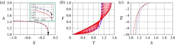
Comparison of the TLM (plain red), STL (dash-dotted blue) and NOR (dashed black) models near a surface slope singularity at
 $X=0$
for
 ${\it\Gamma}=0$
. (a) Backwater curve
 $h(X)$
. (b) Associated velocity profiles
 $T(X)$
. (c) Corresponding curves
 ${\it\Sigma}=h^{\prime }(X)$
as functions of
 $h$
.

Same as figure 4 for
 ${\it\Gamma}=1$
. In contrast to the
 ${\it\Gamma}=0$
case,
 $h_{n}\sim 1.44$
is bounded.

A first comparison between the TLM, STL and NOR models is made for the case of constant slope
 ${\it\Gamma}=0$
. We start with an initial condition with
 $h_{0}$
high enough that
 $T_{0}(Y)$
can be approximated by a parabola. A singularity at finite length is expected as shown in figure 4. The singularities of the three models have been translated to
 $X=0$
in order to compare them. The heights of these backwater curves differ by only 5 %, which is also the order of magnitude of the difference between the critical height
 $h_{c}=1$
of the TLM and STL models and the critical height
 $h_{c}\sim 1.06$
of the NOR model. Similar results are found with non-vanishing slopes
 ${\it\Gamma}\neq 0$
(e.g. figure 5). These flows can be viewed as the fluvial regime of a transcritical transition through a bottom slope discontinuity.
3.2. Phase portraits for semi-parabolic bottom shapes
We now choose a semi-parabolic bottom profile
 $Z_{f}(X)$
such that
 ${\it\Gamma}(X)=-Z_{f}^{\prime }(X)$
reads
 ${\it\Gamma}(X)={\it\xi}X$
for
 $X\geqslant 0$
and
 ${\it\Gamma}(X)=0$
for
 $X\leqslant 0$
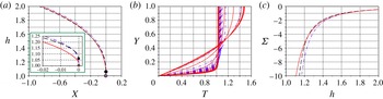
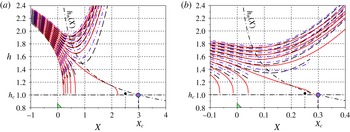
. A comparison of the phase portrait for the TLM, STL and NOR models is shown in figure 6 for two values of
 ${\it\xi}$
. The initial conditions, taken at
 $X=-1$
, are set to explore the vicinity of the TLM critical point reached for
 $X=3$
for
 ${\it\xi}=1$
and
 $X=0.3$
for
 ${\it\xi}=10$
. The initial velocity profile for the TLM is computed from the STL model for the same value of initial height
 $h_{0}$
. A fine tuning of these values (up to twelve digits) shows that
 $({\it\Gamma}_{c},h_{c})\sim (3,1)$
as predicted by our theory.
The negative slope of the critical trajectory in the
 $(X,h)$
plane can be compared to the expression (2.7) that reads here
 $$\begin{eqnarray}{\it\Sigma}_{-}({\it\xi})=\frac{3}{2}\left(1-\sqrt{1+\frac{4{\it\xi}}{27}}\right)=-\frac{1}{9}{\it\xi}+\frac{1}{243}{\it\xi}^{2}+O({\it\xi}^{3}).\end{eqnarray}$$
This can be done visually by considering the curve of the normal height profiles
 $h_{n}(X)=[{\it\Gamma}(X)/3]^{1/3}$
and noticing that
 $h_{n}^{\prime }(X_{c})=-{\it\xi}/9$
. For
 ${\it\xi}=1$
, the proximity of the slopes
 ${\it\Sigma}_{-}(1)\sim h_{n}^{\prime }(X_{c})\sim -0.11$
can be seen in figure 6. For
 ${\it\xi}=10$
, the discrepancy between
 ${\it\Sigma}_{-}(10)=-0.86$
and
 $h_{n}^{\prime }(X_{c})=-1.11$
can be discerned visually.
These backwater phase portraits help to explain why the NOR model fails to catch the correct values of
 ${\it\Gamma}_{c}$
and
 $h_{c}$
. Indeed, the singularities of the phase portraits are associated with plug-like velocity profiles
 $T(Y)$
with
 ${\it\beta}=\int _{0}^{1}T^{2}\,\text{d}Y\rightarrow 1$
while this shape factor is stuck at
 ${\it\beta}=1.2$
for the NOR model.
Phase portrait comparison between the TLM (plain red), the STL (dash-dotted blue) and the NOR (dashed black) models for a parabolic bottom ramp
 $Z_{f}(X)=-{\it\xi}X^{2}/2$
for
 $X\geqslant 0$
and
 $Z_{f}(X)=0$
for
 $X\leqslant 0$
. The normal heights
 $h_{n}(X)$
, defined for
 $X>0$
, are shown by dashed-dotted lines. Determination of the critical point for (a)
 ${\it\xi}=1$
and (b)
 ${\it\xi}=10$
.

3.3. Bottom shape inverse problem and validation of the critical slope relation
Rather than computing the unique critical backwater
 $h(X)$
that links the fluvial and torrential regimes for a given bottom slope profile
 ${\it\Gamma}(X)$
, which is cumbersome, we consider the inverse problem of computing the latter, given the former. This is done by considering that
 ${\it\Sigma}$
and
 ${\it\Gamma}$
are respectively known and unknown in the implicit (3.1).
We choose
 $h(X)=\overline{h}+{\rm\Delta}h\tanh (X/L)$
with
 $\overline{h}=(h_{1}+h_{2})/2$
and
 ${\rm\Delta}h=(h_{2}-h_{1})/2$
such that
 $h_{1}=(3/{\it\Gamma}_{1})^{1/3}$
and
 $h_{2}=(3/{\it\Gamma}_{2})^{1/3}$
are the normal heights associated with the bottom slopes
 ${\it\Gamma}_{2}>{\it\Gamma}_{1}$
. The corresponding
 ${\it\Gamma}(X)$
in the cases
 ${\it\Gamma}_{1}=1$
,
 ${\it\Gamma}_{2}=4$
and
 $L=0.8$
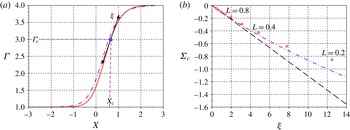
is displayed in figure 7(a) for both the TLM and STL models. Further numerical experiments show that the discrepancy between the two models disappears when
 $L$
increases. We also observe that
 ${\it\Gamma}\sim 3$
when
 $h=1$
, which confirms the value of the critical slope
 ${\it\Gamma}_{c}=3$
. This defines the location
 $X_{c}$
of the critical point. For each value of
 $L$
, we then compute
 ${\it\xi}={\it\Gamma}^{\prime }(X_{c})$
, which traces back the curvature of the bottom at the critical point. Its relation with the critical slope
 ${\it\Sigma}_{c}={\it\Sigma}(X_{c})$
is shown in figure 7(b) and compared (dashed-dotted blue curve) with the function
 ${\it\Sigma}_{-}({\it\xi})$
of (3.2), derived from the STL model. We observe a satisfactory agreement compared to the NOR model, which can only predict a critical slope
 ${\it\Sigma}_{c}=h_{n}^{\prime }(X)=-{\it\xi}/9$
given by the normal height profile
 $h_{n}(X)$
.
Slope
 ${\it\Gamma}(X)$
such that
 $h(X)=\overline{h}+{\rm\Delta}h\tanh (X/L)$
is the critical backwater curve in the cases
 ${\it\Gamma}_{1}=1$
and
 ${\it\Gamma}_{2}=4$
. (a) Comparison between the TLM (plain red) and the STL (dash-dotted blue) for
 $L=0.8$
. (b) Critical surface slope
 ${\it\Sigma}_{c}=h^{\prime }(X_{c})$
as a function of the bottom curvature
 ${\it\xi}={\it\Gamma}^{\prime }(X_{c})$
for
 $L=2^{k/2}/10$
and
 $k=2,3,\ldots ,11$
. Comparison with the theoretical functions for the STL (dash-dotted blue) and the NOR (dashed black) models.

4. Conclusion
We have shown that the STL model, based on a similarity assumption
 $u=T(y/h)/h$
for the streamwise velocity
 $u(X,y)$
, could provide a reasonable approximation of the TLM model that takes into account the
 $X$
-dependency of
 $u=T(X,y/h)/h$
beyond that of the height profile
 $h(X)$
. We proved this to be the case for the critical transition of a laminar shallow-water flow in the presence of a bottom with increasing slope
 ${\it\Gamma}(X)$
. Through numerical simulations of the TLM model, which involve the resolution of an implicit nonlinear differential equation, we have checked the validity of the relation (3.2) between the critical surface slope
 ${\it\Sigma}_{c}=h^{\prime }(X_{c})$
and the bottom curvature factor
 ${\it\xi}={\it\Gamma}^{\prime }(X_{c})$
computed at the critical location
 $X=X_{c}$
.
We have shown that the critical values were
 $h_{c}=1$
and
 ${\it\Gamma}_{c}=3$
for a Newtonian rheology in the laminar case, contrarily to the commonly used NOR model that leads to
 $h_{c}=1.2^{1/3}\sim 1.06$
and
 ${\it\Gamma}_{c}=2.5$
, as shown in § 2.3. Other rheologies would provide different values in the framework of the STL approach. Indeed, these generalizations lead to different functions
 ${\it\alpha}({\it\Delta})=T^{\prime }(0)$
, related to the bottom friction, and
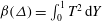 ${\it\beta}({\it\Delta})=\int _{0}^{1}T^{2}\,\text{d}Y$
, related to the shape of the velocity profiles. These functions provide the values of
 $h_{c}^{3}=\lim _{{\it\Delta}\rightarrow \infty }{\it\beta}({\it\Delta})$
and
 ${\it\Gamma}_{c}$
as the solution of
 ${\it\Delta}_{n}={\it\alpha}({\it\Delta}_{n})$
with
 ${\it\Delta}_{n}=h_{c}^{3}{\it\Gamma}_{c}$
. But there is a universality of the critical slope expression through (2.7) that involves only
 $h_{c}$
,
 ${\it\Gamma}_{c}$
and
 ${\it\xi}={\it\Gamma}^{\prime }(X_{c})$
.
The STL model is likely to provide a good approximation of the TLM model for other shallow-water regimes, as is suggested by comparison of the backwater curves of the two models, for instance in the
 $(h,{\it\Sigma})$
representation of figure 3. Such an exhaustive plot in the case of the TLM model could not be shown here due to numerical problems that lead to instabilities or failure of the implicit problem resolution for some regions of the
 $(h,{\it\Sigma})$
plane. Numerical methods to overcome this difficulty are to be explored. This could validate the complex classification of the backwater curves associated with the STL model, due to multiple values of
 ${\it\Sigma}=h^{\prime }(X)$
as a function of
 $h$
for
 ${\it\Gamma}\in [1.82,3]$
.
An extension of our approach to unsteady flows is under way. This could improve the temporal and spatial stability analysis of the normal flows (Thual, Plumerault & Astruc Reference Thual, Plumerault and Astruc2010, and references therein). We think that numerous flow analyses, such as roll waves or hydraulic jumps (Thual Reference Thual2013, and references therein), could be enriched in the light of these TLM and STL shallow-water models. Their generalization to non-Newtonian rheologies and turbulence parameterization is possible. Finally, taking into account capillarity effects in these models is worth pursuing in order to address, with our approach, the vast literature devoted to thin viscous films.
Acknowledgement
This work was performed in the framework of the PHYSCALE project of the RTRA STAE foundation (http://www.fondation-stae.net).