1 Motivation
During the first half of the 20th century, the study of unsteady aerodynamics was motivated by problems associated with wing flutter, the estimation of helicopter blade loads and the effect of wing gusts on airplanes. These problems remain relevant today. Indeed, unsteady blade loads and blade vibrations are still important subjects of helicopter and wind turbine aerodynamics research; and the blades of high speed modern helicopters can experience velocity amplitudes of more than 100 % (Leishman Reference Leishman2000). The interaction of the unsteady effects are not fully understood, hence more precise predictions of the unsteady lift overshoot are required (Leishman & Bagai Reference Leishman and Bagai1998; van Kuik et al. Reference van Kuik, Micallef, Herraez, van Zuijlen and Ragni2014). Moreover, the recent and dramatic rise in wind energy demands robust design of wind turbines – whose blades are exposed to large angle of attack variations and to highly unsteady flows produced by, inter alia, yaw misalignments, atmospheric turbulence and the atmospheric boundary layer – for the prediction of maximum fatigue loads (Barlas & Van Kuik Reference Barlas and Van Kuik2010). Furthermore, wind turbine noise is highly affected by unsteady aerodynamics and noise reduction is an important research field (Wagner, Bareiss & Guidati Reference Wagner, Bareiss and Guidati1996).
The landmark NACA report from Theodorsen (Reference Theodorsen1935) produced a general analytical solution for airfoils encountering oscillating angle of attack variations and oscillating plunge motion. Assuming a potential flow in a steady stream, he calculated all velocity potentials and determined the unsteady circulation, where the wake vorticity is calculated by the Kutta condition. He made use of the following simplifications: flat plate airfoil, two-dimensional incompressible potential flow without viscosity, straight and flat non-deforming wake, small angle assumption and attached flow.
The need for more accurate estimations of helicopter blade loads motivated Isaacs (Reference Isaacs1945) to extend Theodorsen’s work to include an oscillating free stream. Based on Theodorsen’s and Isaacs’ approaches, Greenberg (Reference Greenberg1947) developed a simplified solution for the dynamic lift of a flat plate in an oscillating free stream including an oscillating angle of attack and oscillating plunge motion. In 1991, van der Wall provided an extensive review of existing theoretical approaches and extended Isaacs’ theory to harmonic plunge motion and unsteady angle of attack variations including arbitrary multiples of the free stream harmonic (van der Wall Reference van der Wall1992; van der Wall & Leishman Reference van der Wall and Leishman1994). He concluded that Isaacs’ theory is the only exact theory without additional simplifications. Furthermore, he evaluated the circulatory lift and lift coefficient and found significant deviations of Greenberg’s theory to Isaacs’ theory for free stream oscillation amplitudes higher than
 $\pm$
40 % of the mean velocity.
In light of the advances described above, it is surprising that many of these theories have not been fully validated experimentally, especially for large free stream oscillation amplitudes (Leishman Reference Leishman2002). Favier et al. (Reference Favier, Agnes, Barbi and Maresca1988) investigated a pitching airfoil in an unsteady free stream. The wind tunnel generated high reduced frequencies and moderate velocity amplitudes. Although the airfoil lift with fully attached flow showed significant dynamic effects, a comparison to Isaacs’ theory was not performed. More recently, Granlund et al. (Reference Granlund, Monnier, Ol and Williams2014) experimentally investigated a NACA 0009 over a broad range of reduced frequencies at relatively small velocity amplitudes of 0.1. Other studies examine the pure pitch motion of airfoils. These investigations focus more on the load variations due to deep dynamic stall and the generation of a strong leading edge vortex (Granlund, Ol & Bernal Reference Granlund, Ol and Bernal2013; Bross & Rockwell Reference Bross and Rockwell2014). More recently, symmetric airfoils performing pure pitch motion in fully attached flow were numerically investigated and the influence of their thickness was compared to Theodorsen’s theory (Motta, Guardone & Quaranta Reference Motta, Guardone and Quaranta2015).
It is not clear why this lack of validating Isaacs’, Greenberg’s and van der Wall’s theories exists which includes, besides pitch motion, free stream velocity oscillations. It seems that the existing experimental facilities lack the large amplitude unsteady parameter range. Tunnels that produce an unsteady free stream are rare. The most common approach is to modify a standard steady wind tunnel to produce unsteady flows (Ham, Bauer & Lawrence Reference Ham, Bauer and Lawrence1974; Pierce, Kunz & Malone Reference Pierce, Kunz and Malone1978; Retelle, McMichael & Kennedy Reference Retelle, McMichael and Kennedy1981; Szumowski & Meier Reference Szumowski and Meier1996; Harding, Payne & Bryden Reference Harding, Payne and Bryden2014). Some tunnels combine the independent capabilities of angle of attack and wind speed variation (Favier, Rebont & Maresca Reference Favier, Rebont and Maresca1979; Goodrich & Gorham Reference Goodrich and Gorham2008; Gompertz et al. Reference Gompertz, Jensen, Kumar, Peng, Gregory and Bons2011). Recently, an unsteady wind tunnel was developed to produce large amplitude oscillations of the free stream (Greenblatt Reference Greenblatt2015, Reference Greenblatt2016). Problems of fan stall, large inertial effects and acoustic resonance were overcome during the initial design and testing phases. The tunnel proved to be ideally suited to validate large amplitude unsteady effects and, in particular, to assess the validity of theoretical approaches.
The objective of this paper is to evaluate the theories of Greenberg and Isaacs for large amplitude free stream oscillations, up to 50 %, at different but constant angles of attack on a NACA 0018 airfoil. The dedicated unsteady wind tunnel described by Greenblatt (Reference Greenblatt2015, Reference Greenblatt2016) was exploited for the purpose of generating unsteady surface pressures, or bound vortex sheet strength, and hence variations in the lift coefficient. In order to perform a more meaningful evaluation of the results, the existing theory was extended to calculate the bound, unsteady vortex sheet strength based on van der Wall’s approaches. Comparisons of the measured and theoretical vortex sheet strengths were used as a basis for understanding the limitations of the theory, particularly in the presence of ubiquitous separation bubbles.
2 Theory
As a first step, a sketch of the general set-up is depicted and the final equations of Isaacs and Greenberg are reiterated. Then, the derivation of the wake vortex sheet is briefly described which is based on van der Wall’s approach to generalize Isaacs’ theory. In a final step, the existing theory is extended to enable the prediction of the bound vortex sheet strength.
Sketch of the oscillating inflow (solid arrows), the NACA 0018 which is modelled as a flat plate, the resulting unequally distributed shed wake vorticity
 ${\it\gamma}_{w}$
(black circular arrows) and the resulting induced normal velocities (small dashed arrows).

2.1 Determination of the unsteady lift overshoot due to a sinusoidal free stream
Figure 1 depicts a NACA 0018 immersed in an unsteady free stream (solid arrows). The sinusoidal velocity profile
 $u(t)=u_{s}(1+{\it\sigma}\sin ({\it\omega}t))$
possesses a steady velocity component
 $u_{s}$
and an oscillating component which is scaled by the velocity amplitude
 ${\it\sigma}$
. The velocity varies only in time and is assumed to be constant along the chord. This resembles an airfoil fore–aft motion in an otherwise constant free stream. For the sketch in figure 1, however,
 ${\it\omega}$
depicts the circular frequency of the oscillating free stream. In theory, the airfoil is modelled as a flat plate in incompressible, potential flow. The oscillating free stream
 $u(t)$
causes a variation of the bound airfoil circulation
 ${\it\Gamma}(t)$
. To keep the circulation in the entire system constant (the starting vortex is neglected), a vortex has to be shed at the trailing edge and net vorticity convects in the wake (black, circular arrows). This planar wake vortex sheet
 ${\it\gamma}_{w}$
starts at the trailing edge and runs homogeneously to infinity without any diffusion. Furthermore, any displacement in normal direction due to self-induction or interaction with the bound vortex sheet is neglected. These vortices induce normal velocities
 $v_{n}$
on the flat plate (small dashed arrows) and the bound vortex sheet strength
 ${\it\gamma}_{b}$
has to be adjusted to prohibit normal velocities along the chord. Thus, the airfoil generates an unsteady lift although the angle of attack
 ${\it\alpha}$
is constant. Isaacs’ and Greenberg’s theories are approaches to quantify the unsteady lift overshoot. The entire uneven distributed wake vortex sheet is integrated to determine the current bound vortex sheet. Isaacs and Greenberg assumed that the wavelength of the fore–aft motion is much larger than the chord length
 $c=0.348~\text{m}$
and the two authors used the small angle assumption of the form
 $\sin ({\it\alpha})\approx {\it\alpha}$
to linearize the equations. The velocity amplitude is
 ${\it\sigma}\leqslant 1$
to avoid reverse flow situations.
Besides
 ${\it\sigma}$
, the reduced frequency
 $k={\it\omega}c/2u_{s}$
is the second governing parameter in Isaacs’ and Greenberg’s theories. The resulting unsteady lift is normalized with the steady lift
 $L_{s}={\rm\pi}{\it\rho}cu_{s}^{2}{\it\alpha}$
of a flat plate in potential flow with the given air density
 ${\it\rho}$
(Anderson Reference Anderson2011, p. 329). Although Isaacs and Greenberg focused on the ratio between the unsteady lift
 $L(t)$
and the steady lift
 $L_{s}$
, the ratio of the non-dimensional lift coefficients is considered as the more appropriate parameter for comparison in this study. Thus, all dynamic effects in this paper are quantified by means of the non-dimensional lift coefficient ratio represented in (2.1) which is suggested by van der Wall & Leishman (Reference van der Wall and Leishman1994). Thereby, the quasi-steady lift coefficient merely depends on the square of the velocity and the steady lift (Isaacs Reference Isaacs1945)
 $$\begin{eqnarray}\displaystyle \frac{C_{l}(t)}{C_{l,qs}}=\frac{L(t)}{L_{s}}\frac{1}{(1+{\it\sigma}\sin ({\it\omega}t))^{2}}. & & \displaystyle\end{eqnarray}$$
The results of Isaacs’ theory at constant angle of attack are depicted in (2.2). Isaacs did not imply any additional assumptions regarding the wake. Thus, his results were considered as mathematically exact (van der Wall Reference van der Wall1992). Regarding the lift coefficient in (2.2), the term
 $0.5{\it\sigma}k\cos ({\it\omega}t)$
represents the non-circulatory solution. All other terms represent the circulatory solution which contains the quasi-steady lift and the unsteady wake (depicted by
 $l_{m}$
). Isaacs’ results include two nested summations. The coefficients of the first summation are the real part
 $\text{Re}$
and imaginary part
 $\text{Im}$
of
 $l_{m}$
.
 $$\begin{eqnarray}\displaystyle \hspace{-15.00002pt}\frac{C_{l}(t)}{C_{l,qs}} & \hspace{-2.0pt}=\hspace{-2.0pt} & \displaystyle \frac{1}{(1+{\it\sigma}\sin ({\it\omega}t))^{2}}\left[1+0.5{\it\sigma}^{2}+{\it\sigma}(1+\text{Im}(l_{1})+0.5{\it\sigma}^{2})\sin ({\it\omega}t)\phantom{\mathop{\sum }_{m=2}^{\infty }}\right.\nonumber\\ \displaystyle \hspace{-15.00002pt} & & \displaystyle +\!\left.{\it\sigma}(\text{Re}(l_{1})+0.5k)\cos ({\it\omega}t)+{\it\sigma}\mathop{\sum }_{m=2}^{\infty }(\text{Re}(l_{m})\cos (m{\it\omega}t)+\text{Im}(l_{m})\sin (m{\it\omega}t))\right],\nonumber\\ \displaystyle & & \displaystyle\end{eqnarray}$$
where
 $l_{m}$
is
 $-m(-\text{i})^{m}\sum _{n=1}^{\infty }[F_{n}(J_{n+m}-J_{n-m})+\text{i}G_{n}(J_{n+m}+J_{n-m})]$
and
 $F_{n}$
or
 $G_{n}$
are defined via
 $F_{n}|G_{n}=n^{-2}(J_{n+1}(n{\it\sigma})-J_{n-1}(n{\it\sigma}))F(nk)|G(nk)$
. The two functions
 $F(nk)$
and
 $G(nk)$
are real and imaginary parts of the well-known Theodorsen (Reference Theodorsen1935) function
 $C(nk)=F(nk)+\text{i}G(nk)$
. For very low reduced frequencies
 $k\rightarrow 0$
, the limits are
 $F(nk)\rightarrow 1$
and
 $G(nk)\rightarrow 0$
. If
 ${\it\sigma}$
becomes zero as well, Isaacs’ unsteady lift converges to the steady lift
 $L_{s}$
.
In contrast to Isaacs, Greenberg’s theory included additional assumptions to derive a closed form solution. He used the high-frequency assumption which gives the wake vorticity a harmonic sinusoidal form. This may be questionable because it corresponds to a small
 ${\it\sigma}$
approximation (van der Wall & Leishman Reference van der Wall and Leishman1994). However, using the velocity profile
 $u_{s}$
, Greenberg’s theory leads to the normalized lift coefficient in (2.3).
 $$\begin{eqnarray}\displaystyle \frac{C_{l}(t)}{C_{l,qs}} & = & \displaystyle \frac{1}{(1+{\it\sigma}\sin ({\it\omega}t))^{2}} [\hspace{1.0pt}(1+0.5{\it\sigma}^{2}F)+{\it\sigma}(1+F)\sin ({\it\omega}t)\nonumber\\ \displaystyle & & \displaystyle +\,{\it\sigma}(0.5k+G)\cos ({\it\omega}t)+0.5{\it\sigma}^{2}G\sin (2{\it\omega}t)-0.5{\it\sigma}^{2}F\cos (2{\it\omega}t)].\end{eqnarray}$$
Regarding (2.3), it is obvious that only the first two harmonics are modulated. Due to practical reasons of applicability, Greenberg’s theory was the most used approach for rotorcraft aeroelasticity for many years. Although Greenberg’s approach is convenient due to its simplicity, the high-frequency assumption limits the range of application. van der Wall states that this assumption is equivalent to neglecting the flow oscillation amplitude for the induced velocities. Consequently, the reduced frequency is underestimated for the lower velocities and overpredicted for the higher velocities.
2.2 Derivation of the shed wake vorticity
The lift is an integral force and does not disclose local flow structures along the wing’s chord. In particular, a coupling to the acoustic field requires estimates of the local pressure field. Thus, a new expression for
 ${\it\gamma}_{b}(x,t)$
is derived here. The first step for this purpose is the calculation of
 ${\it\gamma}_{w}$
. The boundary condition of flow tangency requires that the summation of the induced normal velocities of the inflow, the wake vorticity
 $v_{n,w}$
and the bound vorticity
 $v_{n,b}$
is zero in all instances
 $v_{n}(x,t)\equiv 0={\it\alpha}u(t)+v_{n,w}(x,t)-v_{n,b}(x,t)$
. The two equations (2.4) and (2.5), given by van der Wall (Reference van der Wall1992, p. 127), express
 $v_{n,w}$
and
 $v_{n,b}$
and the corresponding Fourier series and the Fourier coefficients
 $b_{n}(t)$
and
 $d_{n}(t)$
in a cylindrical coordinate system (
 $x=0.5c\cos ({\it\Theta})$
), and
 ${\it\gamma}_{b}({\it\theta},t)$
represents the bound vortex sheet strength:
 $$\begin{eqnarray}\displaystyle & \displaystyle v_{n,w}({\it\Theta},t)=-\frac{1}{2{\rm\pi}}\int _{-\infty }^{t}\frac{\dot{{\it\Gamma}}({\it\tau})}{1+{\displaystyle \frac{W(t)-W({\it\tau})}{0.5c}}-\cos ({\it\Theta})}\,\text{d}{\it\tau}={\displaystyle \frac{b_{0}(t)}{2}}+\mathop{\sum }_{n=1}^{\infty }b_{n}(t)\cos (n{\it\Theta}), & \displaystyle \nonumber\\ \displaystyle & & \displaystyle\end{eqnarray}$$
 $$\begin{eqnarray}\displaystyle & \displaystyle v_{n,b}({\it\Theta},t)=\frac{1}{2{\rm\pi}}\int _{0}^{{\rm\pi}}\frac{{\it\gamma}_{b}({\it\theta},t)\sin {\it\theta}}{\cos ({\it\Theta})-\cos ({\it\theta})}\,\text{d}{\it\theta}=\frac{d_{0}(t)}{2}+\mathop{\sum }_{n=1}^{\infty }d_{n}(t)\cos (n{\it\Theta}), & \displaystyle\end{eqnarray}$$
 $$\begin{eqnarray}\displaystyle & \displaystyle {\it\gamma}_{b}({\it\theta},t)=\frac{\displaystyle c_{0}(t)+\mathop{\sum }_{n=1}^{\infty }c_{n}(t)\cos (n{\it\theta})}{\sin ({\it\theta})}, & \displaystyle\end{eqnarray}$$
where
 $W$
is the distance travelled by the airfoil and
 ${\it\tau}$
is an arbitrary instant of time. A comparison of the Fourier series coefficients yields the following identities (Isaacs Reference Isaacs1945, p. 114):
 $c_{0}(t)=2{\it\alpha}u(t)+b_{1}(t)+b_{0}(t);c_{1}(t)=-2{\it\alpha}u(t)+b_{2}(t)-b_{0}(t);c_{n}(t)=b_{n+1}(t)-b_{n-1}(t),n\geqslant 2$
. Furthermore, the Kutta condition has to be fulfilled to determine the correct circulation and is expressed as
 $c_{0}(t)=-\!\sum _{n=1}^{\infty }c_{n}(t)$
(Amiet Reference Amiet1990).
 $c_{0}(t)$
invokes this condition, because
 $b_{n}$
converges to zero for
 $n\rightarrow \infty$
. Isaacs (Reference Isaacs1945, p. 114) and van der Wall (Reference van der Wall1992, p. 130), both present (2.7) for
 $b_{n}(t)$
with the arbitrary travel distance
 ${\it\Lambda}=W(t)-W({\it\tau})$
and the corresponding time derivative of the circulation
 $\dot{Q}(W(t)-{\it\Lambda})=\dot{{\it\Gamma}}(t-T)=\dot{{\it\Gamma}}({\it\tau})$
:
 $$\begin{eqnarray}\displaystyle & \displaystyle b_{n}(t)=-\frac{2}{{\rm\pi}c}\int _{0}^{\infty }\dot{Q}(W(t)-{\it\Lambda})\frac{\left[1+2{\it\Lambda}/c-\sqrt{(1+2{\it\Lambda}/c)^{2}-1}\right]^{n}}{\sqrt{(1+2{\it\Lambda}/c)^{2}-1}}\,\text{d}{\it\Lambda}, & \displaystyle\end{eqnarray}$$
 $$\begin{eqnarray}\displaystyle & \displaystyle \dot{Q}(W(t)-{\it\Lambda})=\mathop{\sum }_{m=-\infty }^{\infty }\frac{A_{m}}{R_{m}}\text{i}m{\displaystyle \frac{{\it\omega}}{u_{s}}}\text{e}^{\text{i}m({\it\omega}/u_{s})(W(t)-{\it\Lambda})}. & \displaystyle\end{eqnarray}$$
Under the assumption that the exogenous variable
 $u(t)$
is periodic in time, the resulting time derivative circulation
 $Q(t)$
in (2.8) is periodic in time as well (
 $m$
is the wavenumber). The most general formulation of the coefficients
 $A_{m},R_{m}$
is given by van der Wall (Reference van der Wall1992, pp. 131–136) (the coefficient
 $\text{i}mk(c/2)$
in (B 41) in (van der Wall Reference van der Wall1992, p. 131) contains a typographical error, the coefficient in front of the integral must be
 $\text{i}mk(2/c)$
. This typo has no consequence for the rest of van der Wall (Reference van der Wall1992)). A closed solution of the unsteady wake vortex sheet for a pure, sinusoidal free stream oscillation is represented by (2.8)–(2.10). Thereby, the terms
 $J$
describe Bessel functions of the first kind
 $$\begin{eqnarray}\displaystyle R_{m}=1+\text{i}mk\frac{2}{c}\int _{0}^{\infty }\text{e}^{-\text{i}m({\it\omega}{\it\Lambda}/u_{s})}\left(\sqrt{\frac{c}{{\it\Lambda}}+1}-1\right)\,\text{d}{\it\Lambda}, & & \displaystyle\end{eqnarray}$$
 $$\begin{eqnarray}\displaystyle A_{0}={\rm\pi}c{\it\alpha}u_{s}\left(1+\frac{{\it\sigma}^{2}}{2}\right);\quad A_{m}=\frac{\text{i}^{m}}{2m}{\rm\pi}c{\it\alpha}u_{s}{\it\sigma}[J_{m+1}(m{\it\sigma})-J_{m-1}(m{\it\sigma})]. & & \displaystyle\end{eqnarray}$$
By means of the known shed vorticity, the circulation of the airfoil is now determined which enables the computation of the unsteady lift. For this purpose, only the two coefficients
 $c_{0}(t)$
and
 $c_{1}(t)$
have to be evaluated.
2.3 Calculation of the unsteady bound vortex sheet strength
The approach to determine the bound unsteady vortex sheet strength is depicted in (2.6). The limit values of the unsteady bound vortex sheet strength at the leading and trailing edge coincide with the steady solution as shown by Strangfeld et al. (Reference Strangfeld, Müller-Vahl, Nayeri, Paschereit and Greenblatt2014). The conjunction between the shed wake and the bound vortex sheet strength is given in (2.8). The sinusoidal velocity profile
 $u(t)$
determines the distance travelled by the airfoil
 $W(t)=\int u(t)\,\text{d}t=u_{s}(t-{\it\sigma}/{\it\omega}\cos ({\it\omega}t))$
, whereas the starting process is not considered. The phase angle
 ${\it\phi}={\it\omega}t$
is introduced for simplification without loss of generality. The substitution
 ${\it\Lambda}=c\tilde{{\it\Lambda}}$
with
 $\text{d}{\it\Lambda}=c\,\text{d}\tilde{{\it\Lambda}}$
simplifies the final equation of
 $b_{n}({\it\phi})$
. Furthermore, the definition of
 $k$
is used and the substitution
 $S_{m}=\text{i}m(2k/c)\text{e}^{\text{i}m({\it\phi}-{\it\sigma}\cos ({\it\phi}))}$
is incorporated in (2.11). A more detailed derivation of the bound vortex sheet strength is given in Strangfeld et al. (Reference Strangfeld, Müller-Vahl, Nayeri, Paschereit and Greenblatt2014)
 $$\begin{eqnarray}\displaystyle b_{n}({\it\phi})=-{\displaystyle \frac{2}{{\rm\pi}}}\mathop{\sum }_{m=-\infty }^{\infty }A_{m}S_{m}{\displaystyle \frac{\displaystyle \int _{0}^{\infty }\text{e}^{-\text{i}mk2\tilde{{\it\Lambda}}}{\displaystyle \frac{\left[1+2\tilde{{\it\Lambda}}-2\sqrt{\tilde{{\it\Lambda}}^{2}+\tilde{{\it\Lambda}}}\right]^{n}}{2\sqrt{\tilde{{\it\Lambda}}^{2}+\tilde{{\it\Lambda}}}}}\,\text{d}\tilde{{\it\Lambda}}}{\displaystyle 1+2\text{i}mk\int _{0}^{\infty }\text{e}^{-\text{i}mk2\tilde{{\it\Lambda}}}\left(\sqrt{{\displaystyle \frac{1}{\tilde{{\it\Lambda}}}}+1}-1\right)\text{d}\tilde{{\it\Lambda}}}}. & & \displaystyle\end{eqnarray}$$
Now, the problem of the unsteady bound vortex sheet strength
 ${\it\gamma}_{b}({\it\theta},t)$
is completely solved. By means of the known coefficients
 $b_{n}$
,
 ${\it\gamma}_{b}({\it\theta},t)$
is determined for all arbitrary amplitudes
 ${\it\sigma}$
and reduced frequencies
 $k$
. Although
 $A_{m}$
,
 $S_{m}$
and the denominator in (2.11) are independent of
 $n$
, the integral in the numerator possesses
 $n$
as an exponent. Thus, for all desired wavenumbers
 $m$
and coefficients
 $b_{n}$
, this equation has to be solved separately. This results in relatively large computation time because several hyperbolic Bessel functions K and confluent hypergeometric Kummer functions M are part of the solution. Exact solutions of the integrals, termed
 ${\it\kappa}(n)$
, for arbitrary
 ${\it\sigma}$
and
 $k$
are given in the appendix A. Numerical values of these integrals for a distinct combination of
 $k$
and
 ${\it\sigma}$
are stated in Strangfeld et al. (Reference Strangfeld, Müller-Vahl, Nayeri, Paschereit and Greenblatt2014).
The integration of the bound vortex sheet strength reveals the circulation which determines the unsteady lift via (2.12) with
 ${\it\Gamma}(t)=\int _{-0.5c}^{0.5c}{\it\gamma}_{b}(x,t)\,\text{d}x$
(Isaacs Reference Isaacs1945, p. 115).
 $$\begin{eqnarray}\displaystyle L(t)={\it\rho}u(t){\it\Gamma}(t)+{\it\rho}\frac{\text{d}}{\text{d}t}\int _{-0.5c}^{0.5c}{\it\gamma}_{b}(x,t)(0.5c-x)\,\text{d}x. & & \displaystyle\end{eqnarray}$$
3 Experimental set-up
Firstly, the airfoil geometry, the unsteady wind tunnel, the used measurement techniques and the data processing are described. Then, a measured sinusoidal velocity profile with an amplitude of 50 % is discussed in detail.
3.1 Airfoil geometry
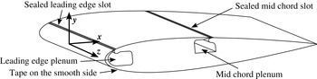
Figure 2 shows a schematic of the two-dimensional NACA 0018 airfoil employed in this study. The chord is
 $c=0.348~\text{m}$
and the span is
 $s=0.61~\text{m}$
yielding an aspect ratio of 1.75. Despite this moderate aspect ratio, CFD simulations via URANS (not shown) have indicated that three-dimensional flow structures due to side wall effects are negligible at the mid-span (Strangfeld et al.
Reference Strangfeld, Rumsey, Müller-Vahl, Greenblatt, Nayeri and Paschereit2015). One side of the airfoil is completely smooth (lower surface in the sketch). The other side features two slots for active flow control (Müller-Vahl et al.
Reference Müller-Vahl, Strangfeld, Nayeri, Paschereit and Greenblatt2015). The width of the slots is 1.2 mm and beneath two plenum chambers are connected. In the current study, no active flow control was used and hence the slots and the inlet of the plenum were sealed externally with Kapton polyamide tape to avoid undesired flow through these slots. To retain the airfoil as symmetric as possible, Kapton polyamide tape was also placed on the smooth surface at the same chordwise position. The tape is approximately
 $75~{\rm\mu}\text{m}$
thick and pasted straight. Thus, above the slot it does not follow the convex shape of the airfoil. Hence, further small discontinuities are induced. This somewhat affected the boundary layer development resulting in a separation bubble close to the trailing edge on the slotted side (positive angles of attack) and near mid-chord on the smooth side (negative angles of attack). The different separation mechanisms led to totally different unsteady lift responses, as will be shown in the subsequent sections. The pressure ports directly below the tape were pierced with a bold needle. Preliminary measurements confirmed that the pressure port geometry was not corrupted noticeably by the tape.
Positive angles of attack indicate that a positive lift is generated (in positive
 $y$
-direction). Hence, the suction side is the side with sealed slots and the smooth surface is the pressure side. In contrast, at negative angles of attack, the smooth side (low surface in figure 2) is the suction side and the side with sealed slots is the pressure side.
Sketch of the two-dimensional NACA 0018 airfoil including the coordinate system and the two sealed slots on the upper surface and tape on the smooth side to retain the airfoil symmetric.

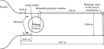
Sketch of the blow-down wind tunnel, the NACA 0018 airfoil equipped with 40 pressure sensors, the hot-wire probes and the louvre mechanism at the end of the test track.

3.2 Experimental set-up and data processing
The blow-down wind tunnel had a cross-section of
 $0.61~\text{m}\times 1.004~\text{m}$
and a 8 : 1 contraction ratio. The maximum achievable free stream velocity is
 $55~\text{m}~\text{s}^{-1}$
with a turbulence level of less than 0.1 % with fully opened louvres. Depending on the blockage ratio of the louvres, the free stream velocity is reduced and the turbulence level may increase up to 0.7 % (Greenblatt Reference Greenblatt2015, Reference Greenblatt2016). The experiments were conducted in the velocity range of
 $7{-}20~\text{m}~\text{s}^{-1}$
. The wind tunnel was powered by a RPM regulated 75 kW radial blower. The blower was specifically designed to operate smoothly under stalled conditions, allowing for a dynamic variation of the wind tunnel speed by adjusting the cross-sectional area of the wind tunnel exit. Louvres controlled the free stream velocity dynamically at the end of the 4.07 m long test track. The distance from the louvres to the trailing edge of the airfoil was approximately 2.8 m, which prevents any inhomogeneities propagating upstream to the airfoil. The louvre mechanism consisted of 13 fully rotatable vanes driven by a 0.75 kW servo motor. The maximum blockage due to the closed louvres amounted to 95 %. A detailed description and reference measurements were published by Greenblatt (Reference Greenblatt2015, Reference Greenblatt2016). Figure 3 shows a schematic of the experimental set-up. The airfoil was placed at the vertical centre of the test section and the leading edge was positioned 0.91 m downstream of the nozzle. The airfoil centre line was equipped with 40 pressure taps with a diameter of 0.8 mm to measure the static pressure at the airfoil surface. The surface pressure was recorded synchronized by means of two ESP-32HD piezoresistive pressure scanners at a sample rate of up to 500 Hz. These two pressure scanners were placed inside the airfoil and each pressure port was connected to the pressure taps by a 44 cm long tube with an internal diameter of 0.8 mm. The phase lag and amplitude attenuation in the tubing were quantified using the method developed by Greenblatt, Kiedaisch & Nagib (Reference Greenblatt, Kiedaisch and Nagib2001). Frequencies from 0 to 50 Hz were examined where both phase lag and amplitude attenuation were found to be negligibly small. This was typically a factor of 50 larger than the frequencies employed for the experiments.
The unsteady free stream velocity in the test section was measured by two hot-wire probes. The data acquisition of the surface pressures and the wind tunnel speed were synchronized, both were recorded at a frequency of 497 Hz. Thus, for each unsteady pressure measurement, the associated free stream velocity was recorded by means of two hot-wire probes upstream of the airfoil. The hot-wire technique prevented any phase lag due to long tubes which rendered the usage of the Pitot tube impractical for the unsteady oscillating free stream. The streamwise phase lag between the velocity measurement at the location of the hot-wires and the trailing edge of the airfoil was estimated to be less than
 $1^{\circ }$
at louvre frequencies of 1 Hz (Greenblatt Reference Greenblatt2015, Reference Greenblatt2016). This is in the range of the measurement accuracy and therefore, the possible phase lag is neglected in this study.
The lift was calculated by means of the 40 pressure taps. The measured static pressure, which acts normal to the surface, was weighted by the half-distance to the neighbouring pressure taps and transformed in the coordinate system of the airfoil chord. The summation yielded the lift, pitching moment and the pressure drag (drag due to friction was not quantified). The blockage ratio of the airfoil amounts to 6 % at zero angle of attack. Only small angles of attack are considered up to
 $\pm 4^{\circ }$
, thus no blockage corrections are computed.
The phase reconstruction was based on the averaged free stream velocity of the two hot-wire probes. Taking into account that the amplitude of the free stream oscillation varied slightly, each single period was fitted individually by an ideal sine to avoid any unphysical scattering in the data. Each measurement consisted of at least 150 periods. The data were averaged at each
 ${\it\alpha}_{step}=0.5^{\circ }$
with a window size of
 $\pm 0.3^{\circ }$
and at each
 ${\it\phi}_{step}=2^{\circ }$
with a window size of
 $\pm 1^{\circ }$
.
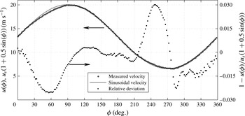
Comparison of the measured free stream velocity
 $u({\it\phi})$
and an ideal sinusoidal free stream velocity
 $u_{s}(1+0.5\sin ({\it\phi}))$
at
 $f=1.2$
Hz,
 $k=0.0985$
,
 $u_{s}=13.32~\text{m}~\text{s}^{-1}$
and
 $\overline{Re}=300\,000$
. The relative deviation is shown on the ordinate on the right-hand side.

3.3 Oscillating free stream
The presented theoretical models of Greenberg as well as Isaacs focused on sinusoidal free stream oscillations. Nevertheless, the fundamental basis for experimentally measured dynamic effects is a precise and accurate adjustment of the time varying free stream velocity
 $u({\it\phi})=u_{s}(1+{\it\sigma}\sin ({\it\phi}))$
. A deviation of
 $u_{s}$
causes mainly an offset of the measured forces. Even more important is the amplitude of the velocity variation
 ${\it\sigma}$
. It has a direct impact on the dynamic effects. Figure 4 shows a representative comparison of the measured phase-averaged free stream velocity and the sinusoidal free stream velocity profile which is assumed in Isaacs’ theory. The corresponding time-averaged Reynolds number was
 $\overline{Re}=300\,000$
and the oscillation frequency was
 $f=1.2~\text{Hz}$
. This results in a reduced frequency of
 $k=0.097$
. As this moderate reduced frequency, unsteady effects, including lift overshoots of more than 25 %, are expected. As already mentioned, the free stream velocity in the test section was controlled by the louvre mechanism at the end of the test track. It is clear from figure 4 that the two velocity profiles were very similar to each other. The ideal time-averaged free stream velocity was
 $\bar{u}_{s,ideal}=13.32~\text{m}~\text{s}^{-1}$
and the measured time-averaged one was
 $\bar{u}_{s,measured}=13.24~\text{m}~\text{s}^{-1}$
, resulting in a deviation of approximately 0.6 %. The desired amplitude was
 ${\it\sigma}=0.5$
and the measured one was
 ${\it\sigma}_{m}=0.506$
. The resulting difference is approximately 1.1 %. Thus, both parameters were considered to be experimentally reproduced with sufficient accuracy. Furthermore, figure 4 depicts the relative divergence for one complete cycle. In the range of
 ${\it\phi}=246^{\circ }$
, an overshoot of almost 3 % is evident although for the other
 ${\it\phi}$
, a slightly undershoot exists. Due to the small differences, they are assumed to be negligible. Hence, the entire free stream velocity profile is expected to be sufficient for dynamic measurements and to be able to reproduce a sinusoidal function. Furthermore, the variations of the free stream velocity lead to a maximum change of the dynamic pressure of around 5 %. To avoid the influence of undesired dynamic pressure deviations, only lift coefficients instead of the total lift are considered in the following.
4 Results
In potential flow, the angular momentum has to remain constant. Due to the unsteady free stream at a constant angle of attack, the lift and the generated circulation of the bound vortex changes. Thus, vortices are shed at the trailing edge to preserve the angular momentum balance. Thereby, the vorticity sheet strength is the time derivation of the circulation changes of the airfoil. In the case of a decreasing free stream velocity, the generated bound circulation decreases as well and the shed vortex possesses the same direction of rotation as the bound vortex. Hence, additional normal velocities on the airfoil are generated which has to be compensated by the stronger bound vorticity sheet. This results in a lift overshoot. Vice versa for an increasing free stream velocity, although the amplitude of the lift deficit is lower because the induced normal velocities of the shed wake vorticity sheet are smaller compared to the current free stream velocity. This is the main idea of the discussed theories and is investigated in the following.
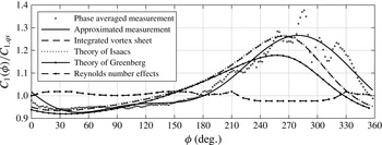
Measured unsteady lift overshoot of a NACA 0018 and the corresponding predictions by integrating the bound, unsteady vortex sheet strength by Isaacs and Greenberg based on a flat plate in potential flow,
 $u(t)=u_{s}(1+0.5\sin ({\it\phi}))$
,
 ${\it\alpha}=2^{\circ }$
,
 ${\it\sigma}=0.5$
,
 $\overline{Re}=300\,000$
,
 $k=0.0985$
, and
 $f=1.2~\text{Hz}$
.

4.1 Theoretical validation of the derived bound, unsteady vortex sheet strength
Although the angle of attack was constant, an unsteady lift overshoot was observed due to the unequal distributed wake vortex sheet. Figure 5 illustrates the measured and predicted normalized lift overshoot. The dashed line with dots quantifies the linearly interpolated Reynolds number effects based on 11 reference measurements at various Reynolds numbers between
 $150\,000<Re<450\,000$
. The maximum effect is 2.4 % which is close to the overall measurement accuracy. Nevertheless, all Reynolds number effects are taken into account during the computations of the measured unsteady lift. The solid dots depict the phase-averaged measured lift coefficient in 5. These values are interpolated by means of a Fourier series, including the first two harmonics, in order to remain consistent with Greenberg’s theory. It is illustrated by the black, solid line. In the range of
 $0^{\circ }<{\it\phi}<180^{\circ }$
, the instantaneous lift is decreased compared to the quasi-steady lift whereas
 $u(t)>u_{s}$
(cf. figure 4). Beyond
 ${\it\phi}=180^{\circ }$
, the lift ratio increases significantly. The maximum lift overshoot of 26.6 % is reached at
 ${\it\phi}=280^{\circ }$
which is in the range of the lowest free stream velocity. Additionally, Isaacs’ and Greenberg’s theories are included with the same input parameters (
 ${\it\sigma}=0.5$
,
 $k=0.0985$
). The predicted maximum lift overshoot by Isaacs (dotted line) is 26.7 % and comparable to the measurements. The minimum and the global trend are almost identical as well. A phase shift of approximately 20
 $^{\circ }$
is visible. In contrast, Greenberg’s theory (solid line with dots) fails to predict the unsteady lift precisely. The overshoot is significantly underpredicted (only 17.9 %) which confirms the statement of van der Wall (Reference van der Wall1992, p. 54) that Greenberg’s theory is not accurate for
 ${\it\sigma}\geqslant 0.4$
due to the high-frequency assumption. However, the reasonably good agreement between experiment and theory confirms Isaacs’ unsteady lift theory for high velocity amplitudes. Furthermore, a theoretical validation of the derived bound, unsteady vortex sheet strength (dashed line) with (
 $n=8$
,
 $m=\pm 8$
) is included (cf. (2.12)). The phase of both lines is identical and the amplitude shows a maximum difference of 0.3 %. Besides deviations due to the numerical integration, the Kutta condition is not satisfied for a finite number of
 $n$
. Although
 ${\it\gamma}_{b}(x,{\it\phi})$
tends towards zero, along the last 0.5 % of the chord, it starts to run towards unphysical values. This behaviour requires the assumption of
 ${\it\gamma}_{b}\,(x\geqslant 0.995,{\it\phi})\equiv 0$
to handle this numerical issue (cf. figure 11 at
 $x/c\geqslant 0.995$
).
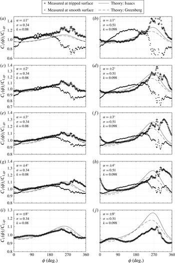
Measured and predicted unsteady lift overshoot for several angles of attack
 ${\it\alpha}$
, two free stream oscillation amplitudes
 ${\it\sigma}$
and two reduced frequencies
 $k$
,
 $u({\it\phi})=u_{s}(1+{\it\sigma}\sin ({\it\phi}))$
,
 $u_{s}=13.32~\text{m}~\text{s}^{-1}$
,
 $\overline{Re}=300\,000$
.

4.2 Comparison of Isaacs’ and Greenberg’s theory with experiments
During the latter part of the phase, namely
 ${\it\phi}\geqslant 240^{\circ }$
, the experimental data are characterized by relatively high-frequency oscillations. Four peaks are discerned in figure 5. These oscillations are caused by the formation and shedding of a trailing edge separation bubble, as will be shown below. In fact, the entire development of the lift variation is intimately related to the nature of the boundary layer separation on the suction surface. To illustrate this point, consider the unsteady lift response for several positive and negative angles of attack shown in figure 6.
The mean Reynolds number is
 $\overline{Re}=300\,000$
and the unsteady free stream follows a sinusoidal function with
 $u({\it\phi})=u_{s}(1+{\it\sigma}\sin ({\it\phi}))$
. Figure 6(a,c,e,g,i) shows an amplitude of
 ${\it\sigma}=0.34$
at a pitch frequency of
 $f=0.098$
Hz which results in a reduced frequency of
 $k=0.08$
. Figure 6(b,d,f,h,j) shows the high free stream oscillation amplitude case with
 ${\it\sigma}=0.51$
at
 $f=1.2$
Hz, resulting in
 $k=0.98$
. The solid lines represent the prediction of Isaacs’ unsteady lift theory and the dashed lines illustrate Greenberg’s theory. The input parameters
 $k$
and
 ${\it\sigma}$
for the theoretical predictions are adapted to the measured velocity oscillation amplitude. The crosses show positive angles of attack, thus the airfoil surface with the sealed slots is the suction side. The dots stand for the corresponding negative angle of attack where the smooth surface is the suction side.
Figure 6(a,c,e,g,i) shows the moderate amplitude case at
 ${\it\sigma}=0.34$
and the predicted maximum lift overshoot is approximately 10 %. At an angle of attack of
 ${\it\alpha}=\pm 1^{\circ }$
, both measurements deviate from the theories. The crosses show a similar global trend but an offset shifts the results to a higher level. The reason for this overshoot is shedding of the trailing edge bubble, and this will be discussed below. The negative angle of attack shows a behaviour that is not only different to the positive angle case, but behaves in totally the opposite manner. At an angle of
 ${\it\alpha}=\pm 2^{\circ }$
, the crosses are in good agreement with the theories. The predicted phase and the amplitude are resembled by the experiments although it is hard to distinguish which theory is closer to the experiments at these low amplitudes. Nevertheless, in the range of
 $240^{\circ }<{\it\phi}<330^{\circ }$
, the scattering in the experimental data increases and a kind of additional high-frequency lift oscillation is visible. The dots for the negative angles of attack still show the odd behaviour, with a deficit in the region of the predicted maximum overshoot. At
 ${\it\alpha}=\pm 3^{\circ }$
, the crosses still agree with the theories. The largest deviations at a positive angle of attack can be seen in the region of the predicted deficit at around
 ${\it\phi}=45^{\circ }$
. At a negative angle of attack, the experiments get close to the theories although a significant deviation exists still. At
 ${\it\alpha}=\pm 4^{\circ }$
, the dots show a phase shift to the theories at approximately
 $300^{\circ }<{\it\phi}<30^{\circ }$
. The maximum lift is shifted by approximately 60
 $^{\circ }$
and no lift deficit in the region of
 $330^{\circ }<{\it\phi}<120^{\circ }$
exists. In fact, the global trend is somehow resembled but the agreement at
 ${\it\alpha}=+4^{\circ }$
is unsatisfying. The lift response at
 ${\it\alpha}=-4^{\circ }$
still shows strong deviations and is not able to capture the lift overshoot appropriately. Additionally, a higher angle of attack of
 ${\it\alpha}=+8^{\circ }$
is shown. At this point, the baseline measurements already show the onset of substantial trailing edge separation with a decreased
 $C_{l}$
versus
 ${\it\alpha}$
slope (Strangfeld et al.
Reference Strangfeld, Müller-Vahl, Nayeri, Paschereit and Greenblatt2014). This violates the Kutta condition and hence the entire potential flow theory. Nevertheless, the unsteady lift response show the same global trend although the amplitude of the measured lift overshoot reduces.
In figure 6(b,d,f,h,j) the high amplitude case is documented at
 ${\it\sigma}=0.51$
and
 $k=0.0985$
. The maximum lift overshoot of Greenberg’s theory amounts to 18 % whereas Isaacs’ predict an overshoot of 26.5 %. At the lowest angle of attack of
 ${\it\alpha}=\pm 1^{\circ }$
, the crosses show significantly higher lift overshoot. It exceeds the ratio of 1.4. The behaviour is probably caused by the low measured differential pressures at this small angle of attack. At the corresponding negative angle of attack, the measured lift response deviates completely from the theories. At
 ${\it\alpha}=\pm 2^{\circ }$
, the measurements at a positive angle of attack agree well with Isaacs’ theory and were already discussed in figure 5. For the negative angles of attack, the experiments and the theories do not agree. At
 ${\it\alpha}=+3^{\circ }$
, the experiments and Isaacs’ theory are similar. The fluctuations of the lift are present and lead to a phase shift of the maximum lift overshoot. Moreover, the minimum lift ratio at approximately
 ${\it\phi}=30^{\circ }$
is not captured adequately anymore. The negative angle of attack still depicts an odd behaviour compared to the theories. At
 ${\it\alpha}=+4^{\circ }$
, the phase shift of the maxima becomes the largest. The entire measured curve seems to have a global phase shifted compared to the theory. Again, the lift deficit is not resembled adequately. Although the lift at the negative angle of attack is far away from the theories, some high-frequency lift fluctuations also occur in the range of
 $240^{\circ }<{\it\phi}<330^{\circ }$
. At the end, the
 ${\it\alpha}=+8^{\circ }$
case is presented as well. As discussed before, the steady baseline measurements already show the onset of trailing edge stall at this angle of attack. Nevertheless, the global trend between experiments and theory is similar. The amplitude of the lift overshoot is reduced whereas the phase is in good agreement. The high-frequency lift oscillations are significantly reduced with only fragments in the form of one distinct peak left. At this angle of attack, the reduced lift coefficient slope of the steady cases already indicates trailing edge separation (Strangfeld et al.
Reference Strangfeld, Müller-Vahl, Nayeri, Paschereit and Greenblatt2014). Besides the effect that this trailing edge separation may reduce the unsteady lift response, it may also suppress the occurrence and shedding of separation bubbles because the flow is already detached. Hence, separation bubble meandering and the high-frequency lift oscillations are significantly reduced. In summary, surveying all of the data at both positive and negative angles of attack in figure 6, it is evident that at positive angles, the trend of the theory is reasonably approximated by the data, while at negative angles the data is in total contradiction to the theory. It will be shown in the subsequent sections that the location, formation and shedding of the separation bubble is responsible for these widely differing results.
Any form of separation violates the potential flow theory and generates deviations to the theories (Timmer Reference Timmer2008; Boutilier & Yarusevych Reference Boutilier and Yarusevych2012). In particular, separation from the trailing edge can have profound effects due to its modification to the Kutta condition. Another trend is that the agreement of experiments and theories is higher for the moderate amplitude case of
 ${\it\sigma}=0.34$
. The high-frequency lift oscillations are reduced and only a minor phase shift exists at
 ${\it\alpha}=+4^{\circ }$
. At high velocity oscillation amplitudes of
 ${\it\sigma}=0.51$
, the high-frequency oscillations in the experiments becomes larger, especially at
 $240^{\circ }<{\it\phi}<330^{\circ }$
. This leads to a significant phase shift which increases with increasing angle of attack. The fairly thick NACA 0018 combined with the highly unsteady free stream may compromise the Kutta condition in some situations (Basu & Hancock Reference Basu and Hancock1978).
Measured and predicted unsteady lift overshoot at
 $u({\it\phi})=u_{s}(1+0.5\sin ({\it\phi}))$
and
 $k\approx 0.98$
for different Reynolds numbers derived from different measurement campaigns. (a)
 ${\it\alpha}=+2^{\circ }$
, (b)
 ${\it\alpha}=+3^{\circ }$
, (c)
 ${\it\alpha}=-2^{\circ }$
, (d)
 ${\it\alpha}=-3^{\circ }$
.

4.3 Reynolds number effects and repeatability
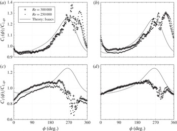
Figure 7 depicts the unsteady lift response for different Reynolds numbers. The crosses represent a mean Reynolds number of
 $\overline{Re}=300\,000$
at a free stream oscillating frequency of 1.2 Hz, resulting in a reduced frequency of
 $k=0.0985$
(comparable to figure 6). The dots in figure 7 possess a mean Reynolds number of
 $\overline{Re}=250\,000$
with an adjusted pitch frequency of
 $f=0.98$
Hz. The resulting reduced frequency is
 $k=0.0965$
. Beside this slight difference of 0.0015, the reduced frequencies are considered to be identical in this comparison.
Due to the oscillating free stream, the strongest Reynolds number effects are expected at
 ${\it\phi}=270^{\circ }$
because at this phase angle the lowest free stream velocities are reached with
 $Re({\it\phi}=270^{\circ })=125\,000$
or 150 000. Furthermore, Isaacs’ theory is plotted for comparison. On the one hand, mean Reynolds numbers below 250 000 are not investigated at this high velocity oscillation amplitude because steady baseline measurements at
 $Re=100\,000$
already show strong Reynolds number effects of more than 10 %. On the other hand, mean Reynolds numbers higher than 300 000 are not measured at this high velocity amplitude. A velocity amplitude of
 ${\it\sigma}=0.5$
leads to a variation in the dynamic pressure of the factor nine. This generates strong structural loads on the wind tunnel walls and the louvres. Thus, the maximum tested mean Reynolds numbers was 300 000 to prevent test facility damages.
At
 ${\it\alpha}=+2^{\circ }$
, the measurements are very similar regarding the amplitude and phase. The high-frequency oscillations occur in both measurements at the same phase angle. Only the peak at around
 ${\it\phi}=324^{\circ }$
has an increased amplitude. Based on this measurement, one might state that these oscillations are a result of Reynolds number effects. At
 ${\it\alpha}=+3^{\circ }$
, the amplitude and the phase angle of the peaks are almost identical. At
 ${\it\phi}=324^{\circ }$
, no significant amplitude differences are detectable. The largest deviations of approximately
 ${\rm\Delta}(C_{l}({\it\phi})/C_{l,qs})=3.5$
% occur in the range of
 $30^{\circ }<{\it\phi}<150^{\circ }$
. This is unexpected because at these phase angles, the maximum Reynolds numbers are generated.
At negative angles of attack, the suction side is smooth and the existence of a laminar boundary layer is likely. At
 ${\it\alpha}=-2^{\circ }$
, both unsteady measurements show the same global trend. High-frequency oscillations occur in the range of
 $260^{\circ }<{\it\phi}<330^{\circ }$
although behaviour is contrary to the theoretical predictions. The high Reynolds number reveals a higher lift ratio which might be a Reynolds number effect. In contrast, at
 ${\it\alpha}=-3^{\circ }$
, both measurements are very similar and no significant differences are present. Even the high frequency oscillations are similar in phase and amplitude.
In conclusion, the variation of Reynolds number of 20 % does not yield general trends. On the one hand, the variation of 20 % is too low to show significant effects. On the other hand, the linear interpolation of eleven baseline measurements in figure 5 reveals a maximum Reynolds number effect of 2 %. Therefore, it is more likely that the Reynolds number does not affect the measurements significantly. More measurements are required to clarify the observed Reynolds number effects.
Measured and predicted unsteady lift overshoot at
 $u({\it\phi})=u_{s}(1+0.5\sin ({\it\phi}))$
and
 $\overline{Re}=250\,000$
for different reduced frequencies
 $k$
. (a)
 ${\it\alpha}=+2^{\circ }$
, (b)
 ${\it\alpha}=+3^{\circ }$
, (c)
 ${\it\alpha}=2^{\circ }$
, (d)
 ${\it\alpha}=3^{\circ }$
.

4.4 Effects of the reduced frequency
The last remaining parameter in the scope of the potential flow theory is the reduced frequency
 $k$
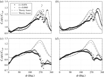
. Figure 8 shows measurements at a mean Reynolds number of
 $\overline{Re}=250\,000$
and at a free stream oscillation amplitude of
 ${\it\sigma}=0.5$
. The frequencies are 0.75 Hz and 1 Hz which result in a reduced frequency of
 $k=0.074$
and
 $k=0.0985$
, respectively. The lower reduced frequency is illustrated as crosses or dashed line. Both lines represent Isaacs’ theory for the corresponding reduced frequencies. The lower
 $k$
produces lower unsteady effects. The measurements at
 $k=0.0985$
illustrated as dots are identical to figure 7.
All measurements with positive angles of attack in figure 8 show globally a similar trend. At the lower
 $k$
, the phase angle of the high-frequency lift peaks is shifted by approximately
 $-15^{\circ }$
compared to the higher
 $k$
case. The absolute amplitude is small for
 $k=0.074$
which is expected because the dynamic in the system is lower. Nevertheless, the amplitude of the high-frequency oscillation is significantly reduced as well at, for example,
 ${\it\phi}=280^{\circ }$
and
 ${\it\phi}=330^{\circ }$
. The minimum lift is reached earlier due to the smaller peak amplitude at an earlier phase angle at
 $k=0.074$
. The theoretical intersection of the lines at
 ${\it\phi}=8^{\circ }$
and
 ${\it\phi}=160^{\circ }$
is also clearly visible in the experiments with a phase shift of approximately
 $+20^{\circ }$
. In conclusion, a higher
 $k$
produces stronger fluctuations and a larger phase lag compared to the theory.
At negative angles of attack, the unsteady lift overshoot behaves contrary to the theory as seen before. Between
 $0^{\circ }<{\it\phi}<180^{\circ }$
, the trend is similar within the measurement accuracy. In the range of
 $180^{\circ }<{\it\phi}=270^{\circ }$
, the higher reduced frequency produces a higher lift coefficient but it is still far away from the theoretical predictions. Nevertheless, between
 $270^{\circ }<{\it\phi}=360^{\circ }$
, high-frequency oscillations occur as well, especially for the higher reduced frequency. A global minimum at
 ${\it\phi}=290^{\circ }$
is reached followed by a local maximum at
 ${\it\phi}=320^{\circ }$
. Thus, the high-frequency lift oscillations seem to be an intrinsic phenomenon in the entire unsteady lift response because it occurs for positive and negative angles of attack although the global behaviour of the lift curves are very different.
As shown, the reduced frequency as well as the free stream oscillation amplitude have a significant effect on the scattering in the experimental data. It cannot be determined finally if these effects are caused only by the pure high dynamics of the system or if additionally the fairly thick airfoil or Reynolds numbers are involved as well.
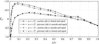
Measured steady pressure distribution at positive and the corresponding negative angles of attack. (a)
 ${\it\alpha}=+3^{\circ }$
,
 $Re=150\,000$
; (b)
 ${\it\alpha}=+2^{\circ }$
,
 $Re=200\,000$
.

4.5 Pressure distributions
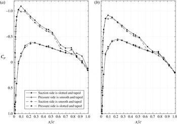
The unsteady lift curves presented in this paper for negative angles of attack exhibit behaviour that deviates radically from the theory. At these angles, the smooth surface of the airfoil is the suction side. However, this uncommon behaviour can be explained by the pressure distribution, which are described in the following. Figure 9 shows the measured pressure distributions at a steady angle of attack of
 ${\it\alpha}=3^{\circ }$
at
 $Re=150\,000$
and
 ${\it\alpha}=2^{\circ }$
at
 $Re=200\,000$
. The solid lines represent the positive angle of attack, the dashed lines the negative one. The circle marker stands for the airfoil side with the sealed slots and the crosses for the smooth side.
At a positive angle of attack of
 ${\it\alpha}=+3^{\circ }$
and
 $Re=150\,000$
, the pressure distribution shows a conventional behaviour in the first half of the airfoil. At
 $0.52<x/c<0.62$
, the slope changes slightly. This might be an effect of the sealed slot at
 $x/c=0.5$
. At
 $x/c=0.78$
, a small bump is visible. This is consistent with the onset of trailing edge stall typified by a small recirculation bubble. At a higher Reynolds number of
 $Re=200\,000$
, all these effects disappear. The suction side shows a continuously smooth and straight trend. Based on these results, some Reynolds number effects exist between
 $150\,000<Re<200\,000$
. Above this range, only minor Reynolds number effects are detectable at positive angles of attack.
At negative angles, the suction side which is in this case the smooth airfoil surface reveals some unexpected results. No clear suction peak exists, only a low-pressure plateau arises at
 $0.05<x/c<0.14$
. The pressure port at
 $x/c=0.08$
yields a higher pressure as the two neighbouring ones although at this position the lowest pressure would be expected as shown for the positive angles of attack. At
 $x/c=0.52$
, a clear pressure rise is visible, although no slots exist on this side, and this is consistent with a mid-chord separation bubble. From this position to the trailing edge, the suction side pressure is equal or even higher than the pressure side, and this is due to a bubble near the trailing edge on the pressure surface. Thus, these shown steady pressure distributions at negative angles of attack indicate strong Reynolds number effects as well as leading edge and mid-chord separation bubbles. The formation and shedding of this mid-chord bubble has a dramatic effect on the surface pressures, and hence vortex sheet, and ultimately the lift variation as will be shown below.
These results strongly indicate that the slots sealed with thin tape at
 $x/c=0.5$
act to modify the boundary layer. The extent to which the tape at
 $x/c=0.05$
affects the boundary layer is not clear, but it certainly does modify the leading edge bubble. Leading edge recirculation bubbles are suppressed and only minor Reynolds number effects are measured. On the contrary, the smooth surface seems to generate a laminar separation bubble close to the leading edge and at mid-chord, and is strongly affected by Reynolds number changes. It will be shown below by means of the unsteady vortex sheet how these factors combine to produce radical deviations of the experiments to Isaacs’ theory for negative angles of attack.
Unsteady pressure distribution at
 ${\it\alpha}=\pm 2^{\circ }$
,
 $\overline{Re}=300\,000$
,
 $k=0.0985$
,
 ${\it\sigma}=0.5$
and
 ${\it\phi}=258^{\circ }$
.

Besides the steady pressure distributions, the unsteady pressure distribution may also give a more detailed insight into the flow around the airfoil. Figure 10 shows the unsteady pressure distribution at an oscillating inflow at mean Reynolds number of
 $\overline{Re}=300\,000$
,
 $k=0.0985$
,
 ${\it\sigma}=0.5$
and
 ${\it\alpha}=\pm 2^{\circ }$
. The chosen phase angle is
 ${\it\phi}=258^{\circ }$
because at this position a significant lift overshoot is measured, the experiments and the theory agree sufficiently, and the unsteady lift is not yet influenced by the high-frequency lift oscillation (see figure 6). The current Reynolds number in this plot is
 $Re=153\,200$
. At a positive angle, the unsteady pressure distribution shows an expected result. The suction side possesses a lower pressure than the pressure side and the curves have a smooth trend. Only at
 $x/c=0.78$
a small bump is recorded. At a negative angle of
 ${\it\alpha}=-2^{\circ }$
, the unsteady pressure distribution is distinctly different. According to the steady measurements, a low-pressure plateau arises close to the leading edge. At
 $x/c=0.52$
, the slope of the pressure distribution changes significantly on the suction side. The same happens at
 $x/c=0.78$
on the pressure side. It seems that both airfoil surfaces are affected by the separation downstream on the aft part of the airfoil. This results in a region of negative lift at
 $0.63<x/c<0.85$
. This region vary strongly in size and position for different phase angles, especially at low unsteady free stream velocities. This phenomenon definitely influences the unsteady lift response and further discussed below by means of the unsteady vortex sheet.
Comparison of the unsteady bound vortex sheet strength
 ${\it\gamma}_{b}$
of a NACA 0018 (measured) and a flat plate in potential flow at
 ${\it\phi}=246^{\circ }$
,
 ${\it\alpha}=3^{\circ }$
,
 ${\it\sigma}=0.5$
,
 $\overline{Re}=300\,000$
,
 $f=1.2$
Hz,
 $k=0.0985$
,
 $n=8$
and
 $m=\pm 16$
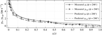
. The quasi-steady
 ${\it\gamma}_{b}$
relates to
 $u({\it\phi}=246^{\circ })/u_{s}=0.543$
.

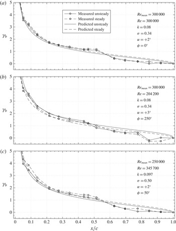
Comparison of the measured and predicted unsteady bound vortex sheet strength
 ${\it\gamma}_{b}$
at
 $n=8$
and
 $m=\pm 16$
.

4.6 Experimental validation of the derived bound, unsteady vortex sheet strength
Figure 11 shows the unsteady and the quasi-steady bound vortex sheet strength
 ${\it\gamma}_{b}$
. The solid line is based on the presented approach and the dashed line is given by Birnbaum (Reference Birnbaum1923, p. 291). The lines with circles are measurements of the vortex strength based on the measured pressure difference
 ${\it\gamma}_{b}={\rm\Delta}p/({\it\rho}u(t))$
. The phase angle is
 ${\it\phi}=246^{\circ }$
,
 ${\it\alpha}=2^{\circ }$
,
 ${\it\sigma}=0.5$
,
 $\overline{Re}=300\,000$
and
 $k=0.0985$
. The two unsteady
 ${\it\gamma}_{b}$
are above the quasi-steady ones, which is consistent with the lift overshoot of more than 20 % at this phase angle. In the range of
 $0.08<x/c<0.5$
, the two unsteady vortex sheet strengths are almost identical. The measured and the quasi-steady vortex sheet strength show a good agreement in the forepart of the airfoil as well. The identical difference between unsteady and quasi-steady conditions results in the already discussed identical lift overshoot. Beyond
 $x/c>0.5$
, some differences occur which may be caused by the thickened boundary layer or by the low differential pressures measured in the rear part of the airfoil. However, the overall agreement of the bound, unsteady vortex sheet strength is sufficient. Thus, the developed theoretical approach for predicting
 ${\it\gamma}_{b}(x,t)$
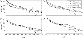
is considered to be correct. This gives a deeper insight into the unsteady flow physics and the spatial development of the unsteady lift overshoot. For instance, the transient change from lift loss to a lift overshoot begins at the trailing edge and the vortex sheet enhancement propagates upstream towards the leading edge. During the transition from a lift overshoot to a lift loss, the lift decrease starts at the trailing edge and propagates upstream as shown by Strangfeld et al. (Reference Strangfeld, Müller-Vahl, Nayeri, Paschereit and Greenblatt2014). Figure 12 depicts the comparison of the predicted and measured vortex sheet strength for three selected cases. In all three cases, the global trend of the measurements and the theory agrees. In the first and the third case, the measured and predicted unsteady lifts reveal a deficit (see figures 6 and 7). In these two cases, the unsteady vortex sheet strength is smaller than the steady one. In the second case, at this given phase angle, a lift overshoot is observed (see figures 6). Here, the unsteady vortex sheet strength is larger than the steady one, as expected. In the first half of the airfoil, the absolute values and the differences between the steady and the unsteady vortex sheet strength agree well between theory and experiments. In parts, the measured and predicted vortex sheet strength are identical. In the rear part of the airfoil, the vortex sheet strength becomes more scattered. Downstream of
 $x/c=0.5$
, the curvature of the measured strength shows a kink. This is due to the pressure side separation bubble that produces a low-pressure region. At
 $0.63<x/c<0.7$
, the measured steady and unsteady vortex sheet strength fall together. Downstream of
 $x/c=0.7$
, the vortex sheet strength shows again partly the predicted differences between steady and unsteady vortex sheet strength. In particular at the lowest Reynolds number in the second case, the steady and the unsteady vortex sheet strength reveal a negative vortex sheet strength at
 $x/c=0.85$
. This is consistent with the low pressure in the pressure surface bubble. Furthermore, these fluctuations of the measured vortex sheet strength in the rear part of the airfoil are suspected to generate the high-frequency lift oscillations as well as the phase lag of the measured and predict lifts (see figures 6).
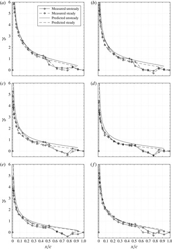
Comparison of the measured and predicted unsteady bound vortex sheet strength
 ${\it\gamma}_{b}$
at
 ${\it\alpha}=-2^{\circ }$
,
 ${\it\sigma}=0.5$
,
 $k=0.0985$
,
 $\overline{Re}=300\,000$
,
 $n=8$
and
 $m=\pm 16$
. (a)
 ${\it\phi}=180^{\circ }$
, (b)
 ${\it\phi}=210^{\circ }$
, (c)
 ${\it\phi}=240^{\circ }$
, (d)
 ${\it\phi}=270^{\circ }$
, (e)
 ${\it\phi}=300^{\circ }$
, (f)
 ${\it\phi}=330^{\circ }$
.

4.7 Unsteady laminar separation bubbles and their influence on the unsteady lift
The discussed unsteady pressure distributions already showed distinct differences between positive and negative angles of attack. To evaluate the influence of the laminar separation bubble at negative angles of attack, the unsteady vortex sheet in considered in more detail. This explains the high deviations of the experiments to Isaacs’ theory at negative angles of attack and shows significant differences between quasi-steady and unsteady laminar separation bubbles.
To understand these dramatic deviations, particularly for
 ${\it\phi}>180^{\circ }$
at negative angles of attack (figure 6), we compare the experimental and theoretical bound vortex sheets at
 ${\it\alpha}=2^{\circ }$
for the phase angles
 ${\it\phi}=180^{\circ }$
to
 ${\it\phi}=330^{\circ }$
in 30
 $^{\circ }$
increments in figure 13. Although the discussion below corresponds specifically to
 ${\it\alpha}=-2^{\circ }$
at
 ${\it\sigma}=0.51$
, (figure 6
d), it also pertains to the other cases, as will be pointed out.
At
 ${\it\phi}=180^{\circ }$
in figure 13, the correspondence between the unsteady and quasi-steady vortex sheet strengths upstream of
 $x/c=0.43$
is reasonable. However, downstream of this, the vortex sheet signature clearly indicates the mid-chord bubble described above in figure 9. Note that the strength of the bubble is significantly stronger than its quasi-steady counterpart. Downstream of the bubble, further aft on the airfoil the differences between the unsteady and steady data are comparable to the theory. Hence the overall, or integral, result is a comparable lift coefficient ratio at this phase angle (see figure 6). As the free stream velocity, and hence Reynolds number, decreases (
 ${\it\phi}=210^{\circ }$
in figure 13), the relative bubble strength increases. By this we mean that the small pressure rise observed previously between
 $x/c=0.34$
and
 $x/c=0.43$
(cf.
 ${\it\phi}=180^{\circ }$
in figure 13) is now a small pressure drop and the differences between steady and unsteady pressures within the bubble are greater. Further aft of the suction surface bubble the differences between steady and unsteady data diminish and overall this is reflected as the beginning of the deviation between data and theory (see figure 6). Significantly, at
 ${\it\phi}=240^{\circ }$
in figure 13, the bubble begins to burst as evident from the vortex signature that shows a pressure rise just downstream of the mid-chord. By
 ${\it\phi}=270^{\circ }$
the bubble appears to have fully shed from the surface as can be seen by the near correspondence of the steady and unsteady data and, as expected, the deviation from the theory is large (figure 6). The shedding of the mid-chord bubble has profound consequences for the remainder of the flow development. At
 ${\it\phi}=300^{\circ }$
, the unsteady sheet strength is now less that its steady counterpart along the entire chord length. This scenario remains mostly unchanged at
 ${\it\phi}=330^{\circ }$
such that at the start of the cycle (
 ${\it\phi}=360^{\circ }$
or 0
 $^{\circ }$
) the lift coefficient is underpredicted. The above description applies to all data sets between
 $-4^{\circ }<{\it\alpha}<4^{\circ }$
for
 ${\it\sigma}=0.34$
and 0.5. The quantitative differences result primarily from the differences in formation and shedding of the mid-chord separation bubble.
It surmized here that both the reduction in Reynolds number and the flow deceleration play a part in the shedding of the bubble. It is well known that separation bubbles play a major, if not dominant, role in determining the aerodynamic performance of low flight Reynolds number airfoils (Mueller Reference Mueller1989). Hence the dramatic differences in lift variation, depending upon whether the separation is at the trailing edge (positive angles here) or mid-chord (negative angles here) will have major consequences for low Reynolds number airfoils subjected to unsteady flows (Ol Reference Ol2007). Furthermore, many certain wind turbine airfoils, that are routinely subjected to highly unsteady flows are designed to incorporate mid-chord separation bubbles (Somers Reference Somers1997). Hence the development of theoretical or computational methods to better understand these phenomena would be of great value.
4.8 Interaction of the vortex sheet and the Kutta condition due to the shedding of a recirculation bubble upstream of the trailing edge
The increased oscillations of the measured lift overshoot in figure 5 in the range of
 $240^{\circ }<{\it\phi}<340^{\circ }$
is caused by the flow physics close to the trailing edge as shown in figure 12. Figure 14 illustrates the unsteady vortex sheet strength for four phase angles. At
 ${\it\phi}=258^{\circ }$
, peak at
 $x/c=0.78$
indicates the existence of separated flow or a recirculation bubble. In the vicinity of this peak, the vortex sheet strength is significantly reduced and below the theoretical one. At
 ${\it\phi}=286^{\circ }$
, the vortex sheet strength is smooth which indicates that recirculation bubble is shed downstream towards the trailing edge. This phenomenon directly affects the Kutta condition and the upstream pressure distribution. Thus, almost the entire measured vortex sheet strength is elevated above the theoretical one, which explains the measured, additional lift overshoot. At
 ${\it\phi}=294^{\circ }$
, the recirculation bubble is shed already in the wake and induces negative normal velocities which reduces the vortex sheet strength. Now, the measured values are below the predicted ones, hence, the measured lift overshoot is reduced significantly. At
 ${\it\phi}=294^{\circ }$
, a new recirculation bubble at
 $0.55<x/c<0.85$
is formed. The shed process is finished and the corresponding reduced frequency of the entire process is approximately 0.7. Further investigations have to reveal if this phenomenon is a low Reynolds number or thick airfoil effect.
Comparison of the measured (with circles) and predicted (no line marker) bound, unsteady vortex sheet strength,
 ${\it\alpha}=2^{\circ }$
,
 ${\it\sigma}=0.5$
,
 $\overline{Re}=300\,000$
,
 $k=0.0985$
,
 $n=8$
and
 $m=\pm 16$
. (a)
 ${\it\phi}=258^{\circ }$
, (b)
 ${\it\phi}=286^{\circ }$
, (c)
 ${\it\phi}=294^{\circ }$
, (d)
 ${\it\phi}=320^{\circ }$
.

4.9 Lift increase due to pressure side bubble bursting
The interpretation of the unsteady pressure data presented here involved a degree of speculation because, on the one hand, the tripping was different on the suction and pressure surfaces and on the other, the no direct flow field measurements were made. Indeed, an additional reason for the large differences between quasi-steady and unsteady results in figure 14 and for the fundamental differences between positive and negative angles (figure 6) can be explained by bursting of the pressure side bubble as a result of low Reynolds number and unsteady effects. Bursting of the pressure side bubble result in an increase in lift as compared to the steady case and this might explain the higher lift coefficients observed in figure 6. This may also explain the higher local loading observed for the unsteady case in figure 14. For negative angles, the slots are on the pressure side and these disturbances may promote transition further upstream. As a consequence, the length of the pressure side separation bubble is decreased and bubble bursting may be avoided. Concurrently, lift increasing effect of the bursting bubble is now absent and the lift coefficient, as shown in figure 6, is smaller.
5 Separation of the ‘impulsive pressure lift’ and the ‘circulatory’ lift
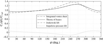
The derived unsteady vortex sheet strength is satisfactorily validated via integration and comparison with Isaacs’ unsteady lift theory as shown by the near identical results as shown in figure 5. Based on these promising results, the presented extension of Isaacs’ theory in form of the unsteady vortex sheet strength is considered to be correct. Accurate evaluation of the complete chordwise bound vortex sheet strength enables a separation of the total lift into two parts, namely the ‘impulsive pressure’ lift (also known as the ‘apparent mass term’) and the ‘circulatory’ lift (also known as ‘Joukowski’ lift) as suggested for example by Isaacs (Reference Isaacs1945) and van der Wall (Reference van der Wall1992).
Separation of the total unsteady lift overshoot into the ‘Joukowski’ lift and the ‘impulsive pressure lift’ via the theoretical unsteady bound vortex sheet strength at
 $k=0.0985$
and
 ${\it\sigma}=0.0567$
.

Besides the theory of Isaacs and its extension derived here, figure 15 depicts the computed ‘impulsive pressure’ lift and the ‘circulatory’ lift at
 $k=0.0985$
and
 ${\it\sigma}=0.5067$
. The latter is defined as
 $L_{J}({\it\phi})={\it\rho}u({\it\phi}){\it\Gamma}({\it\phi})$
and expresses the product of the current free stream velocity times the current circulation generated by the flat plate. It is illustrated by the dashed line in the figure. As can be seen, the pure consideration of the ‘circulatory’ lift would lead to a much stronger amplitude of the unsteady lift response. Furthermore, the maximum possesses another phase angle compared to Isaacs’ theory. The ‘impulsive pressure lift’ is defined as
 $L_{I}({\it\phi})={\it\rho}\text{d}/\text{d}{\it\phi}\int _{-0.5c}^{0.5c}{\it\gamma}_{b}({\it\phi},t)(0.5c-x)\,\text{d}x$
. If only quasi-steady changes are considered, the ‘impulsive pressure lift’ is zero. Thus, in the unsteady case, the ‘impulsive pressure lift’ (dotted line) fluctuates around zero. The minimum is reached at approximately
 ${\it\phi}=240^{\circ }$
and beyond this point the ‘impulsive pressure lift’ increases rapidly to its maximum at around
 ${\it\phi}=330^{\circ }$
. This causes a reduction of the total lift overshoot compared to the ‘circulatory’ lift and promotes a phase shift of the maximum lift ratio. Thus, for the cases considered in this paper, the ‘impulsive pressure’ lift plays a small, but important, role in the prediction of the unsteady lift.
6 Conclusion
This paper considered two aspects of airfoil aerodynamics in the presence of an oscillating free stream hitherto not considered. Firstly, the well-known theory developed by Isaacs was augmented by explicit calculation of the unsteady vortex sheet strength; and secondly, high amplitude experiments were performed on a NACA 0018 airfoil in order to evaluate the theoretical results. The closed form theoretical result for the vortex sheet is valid for arbitrary reduced frequencies and amplitudes and its integration reproduced the lift results of Isaacs. The experiments were unprecedented in terms of Reynolds number and velocity amplitude and were considered to be an appropriate vehicle for evaluation of the theory.
The experiments revealed that seemingly small differences in the separation bubble location on the airfoil suction surface led to dramatically different results. For the case where the boundary layer was tripped, the lift coefficient exhibited an overshoot, similar to the theory. However, near the maximum lift coefficient overshoot, the data revealed a high-frequency oscillation, the cause of which was the formation and shedding of a recirculation bubble near the trailing edge that modified the Kutta condition. This shedding was mainly a result of the flow deceleration, which served to destabilize the bubble, although the relatively low Reynolds number associated with the decreasing freestream may also play a role.
For the case where the boundary layer is not tripped, the strengthening and shedding of the mid-chord separation bubble produced a dramatically different effect. Instead of a lift coefficient overshoot, as the theory suggests, the data exhibited a significant undershoot. This undershoot was also accompanied by high-frequency oscillations that characterized by the bubble shedding.
We can conclude from this work that caution should be exercised when using unsteady flow theory for low Reynolds number airfoil flows. The location of the separation bubble and its subsequent shedding play decisive roles in the resulting aerodynamic loads. The breakdown of the Kutta condition, associated with bubble shedding, renders the theory either approximate or utterly inappropriate. A meaningful validation of the existing theory should be attempted with a relatively thin airfoil where the minimum Reynolds number exceeds
 $10^{6}$
.
Nomenclature

Acknowledgements
The authors are grateful to Professor P. P. Friedmann for bringing their attention to this problem, to Professor B. G. van der Wall for his support and the kind email contacts, and to Dr S. Born for helping to solve the integro–differential equations. This research was supported in part by the Israel Science Foundation (grant no. 840/11) and by the ‘Stiftung der deutschen Wirtschaft’.
Appendix A
The unsteady vorticity sheet
 ${\it\gamma}_{b}({\it\phi})$
is computed via (2.11). This includes two integrals. The function
 ${\it\kappa}$
represents the integral in the numerator in (2.11). The following equations depict their solutions for
 $0\leqslant n\leqslant 7$
for arbitrary
 $k$
and
 $m$
.
 $$\begin{eqnarray}\displaystyle {\it\kappa}(n) & = & \displaystyle \int _{0}^{\infty }\text{e}^{-\text{i}mk2\tilde{{\it\Lambda}}}\frac{\left[1+2\tilde{{\it\Lambda}}-2\sqrt{\tilde{{\it\Lambda}}^{2}+\tilde{{\it\Lambda}}}\right]^{n}}{2\sqrt{\tilde{{\it\Lambda}}^{2}+\tilde{{\it\Lambda}}}}\,\text{d}\tilde{{\it\Lambda}},\end{eqnarray}$$
 $$\begin{eqnarray}\displaystyle {\it\kappa}(n=0) & \Rightarrow & \displaystyle 0.5\text{e}^{\text{i}km}K(0,\text{i}km),\end{eqnarray}$$
 $$\begin{eqnarray}\displaystyle {\it\kappa}(n=1) & \Rightarrow & \displaystyle 0.5\text{e}^{\text{i}km}K(0,\text{i}km)-\text{i}\frac{-2+\sqrt{{\rm\pi}}M(0.5,0,2\text{i}km)}{4km},\end{eqnarray}$$
 $$\begin{eqnarray}\displaystyle {\it\kappa}(n=2) & \Rightarrow & \displaystyle \frac{4+4\text{i}km+\text{e}^{\text{i}km}k^{2}m^{2}({\rm\pi}Y(2,km)+2J(2,km)(\log (\text{i}km)-\log (km)))}{4k^{2}m^{2}},\nonumber\\ \displaystyle & & \displaystyle\end{eqnarray}$$
 $$\begin{eqnarray}\displaystyle {\it\kappa}(n=3) & \Rightarrow & \displaystyle -0.5\left(-7\text{e}^{\text{i}km}K(0,\text{i}km)+\frac{6}{km}\text{e}^{\text{i}km}(\text{i}+km)K(1,\text{i}km)\right.\nonumber\\ \displaystyle & & \displaystyle +\,\frac{\text{i}}{8k^{3}m^{3}} (64+64\text{i}km-24k^{2}m^{2}-18\sqrt{{\rm\pi}}M(-0.5,-2,2\text{i}km)\nonumber\\ \displaystyle & & \displaystyle -\!\left.\vphantom{\frac{6}{km}}15\sqrt{{\rm\pi}}K(0.5,-2,2\text{i}km)+12k^{2}m^{2}\sqrt{{\rm\pi}}M(0.5,0,2\text{i}km))\right),\end{eqnarray}$$
 $$\begin{eqnarray}\displaystyle {\it\kappa}(n=4) & \Rightarrow & \displaystyle \frac{1}{32k^{4}m^{4}} (-768-768\text{i}km+320k^{2}m^{2}+64\text{i}k^{3}m^{3}\nonumber\\ \displaystyle & & \displaystyle +\,16\text{e}^{\text{i}km}k^{2}m^{2}(-21+14\text{i}km+13k^{2}m^{2})K(0,\text{i}km)\nonumber\\ \displaystyle & & \displaystyle -\,32\text{e}^{\text{i}km}km(-21\text{i}-14km+13\text{i}k^{2}m^{2}+6k^{3}m^{3})K(1,\text{i}km)\nonumber\\ \displaystyle & & \displaystyle +\,168\text{i}km\sqrt{\text{i}}M(-0.5,-2,2\text{i}km)+105\sqrt{{\rm\pi}}M(0.5,-3,2\text{i}km)\nonumber\\ \displaystyle & & \displaystyle +\,120\text{i}km\sqrt{{\rm\pi}}M(0.5,-2,2\text{i}km)-32\text{i}k^{3}m^{3}\sqrt{{\rm\pi}}M(0.5,0,2\text{i}km)),\end{eqnarray}$$
 $$\begin{eqnarray}\displaystyle {\it\kappa}(n=5) & \Rightarrow & \displaystyle -0.5\left(-3k^{-2}m^{-2}\text{e}^{\text{i}km}(-45+30\text{i}km+7k^{2}m^{2})K(0,\text{i}km)\vphantom{\frac{\text{i}}{32k^{5}m^{5}}}\right.\nonumber\\ \displaystyle & & \displaystyle +\,k^{-3}m^{-3}10\text{e}^{\text{i}km}(-27\text{i}-18km+11\text{i}k^{2}m^{2}+2k^{3}m^{3})K(1,\text{i}km)\nonumber\\ \displaystyle & & \displaystyle +\,\frac{\text{i}}{32k^{5}m^{5}} (-12\,288-12\,288\text{i}km+5376k^{2}m^{2}+1280\text{i}k^{3}m^{3}-160k^{4}m^{4}\nonumber\\ \displaystyle & & \displaystyle +\,3150\sqrt{{\rm\pi}}M(-0.5,-4,2\text{i}km)-960k^{2}m^{2}\sqrt{{\rm\pi}}M(-0.5,-2,2\text{i}km)\nonumber\\ \displaystyle & & \displaystyle +\,945\sqrt{{\rm\pi}}M(0.5,-4,2\text{i}km)+1050\text{i}km\sqrt{{\rm\pi}}M(0.5,-3,2\text{i}km)\nonumber\\ \displaystyle & & \displaystyle -\!\left.\vphantom{\frac{\text{i}}{32k^{5}m^{5}}}600k^{2}m^{2}\sqrt{{\rm\pi}}M(0.5,-2,2\text{i}km)+80k^{4}m^{4}\sqrt{{\rm\pi}}M(0.5,0,2\text{i}km))\right),\end{eqnarray}$$
 $$\begin{eqnarray}\displaystyle {\it\kappa}(n=6) & \Rightarrow & \displaystyle \frac{1}{128k^{6}m^{6}} (245\,760+245\,760\text{i}km-110\,592k^{2}m^{2}-28\,672\text{i}k^{3}m^{3}+4480k^{4}m^{4}\nonumber\\ \displaystyle & & \displaystyle +\,384\text{i}k^{5}m^{5}+64\text{e}^{\text{i}km}k^{4}m^{4}(-507+338\text{i}km+31k^{2}m^{2})K(0,\text{i}km)\nonumber\\ \displaystyle & & \displaystyle -\,128\text{e}^{\text{i}km}k^{3}m^{3}(-507\text{i}-338km+184\text{i}k^{2}m^{2}+15k^{3}m^{3})K(1,\text{i}km)\nonumber\\ \displaystyle & & \displaystyle -\,58\,590\sqrt{{\rm\pi}}M(-0.5,-5,2\text{i}km)-52\,080\text{i}km\sqrt{{\rm\pi}}M(-0.5,-4,2\text{i}km)\nonumber\\ \displaystyle & & \displaystyle +\,4320\text{i}k^{3}m^{3}\sqrt{{\rm\pi}}M(-0.5,-2,2\text{i}km)-10\,395\sqrt{{\rm\pi}}M(0.5,-5,2\text{i}km)\nonumber\\ \displaystyle & & \displaystyle -\,11\,340\text{i}km\sqrt{{\rm\pi}}M(0.5,-4,2\text{i}km)+6300k^{2}m^{2}\sqrt{{\rm\pi}}M(0.5,-3,2\text{i}km)\nonumber\\ \displaystyle & & \displaystyle +\,2400\text{i}k^{3}m^{3}\sqrt{{\rm\pi}}M(0.5,-2,2\text{i}km)-192\text{i}k^{5}m^{5}\sqrt{{\rm\pi}}M(0.5,0,2\text{i}km)),\end{eqnarray}$$
 $$\begin{eqnarray}\displaystyle {\it\kappa}(n=7) & \Rightarrow & \displaystyle -0.5\left(-\text{e}^{\text{i}km}k^{-2}m^{-2}(-1449+966\text{i}km+43k^{2}m^{2})K(0,\text{i}km)\vphantom{\frac{\text{i}}{128k^{7}m^{7}}}\right.\nonumber\\ \displaystyle & & \displaystyle +\,k^{-3}m^{-3}42\text{e}^{\text{i}km}(-69\text{i}-46km+24\text{i}k^{2}m^{2}+k^{3}m^{3})K(1,\text{i}km)\nonumber\\ \displaystyle & & \displaystyle +\,\frac{\text{i}}{128k^{7}m^{7}} (5898\,240+5898\,240\text{i}km-2703\,360k^{2}m^{2}-737\,280\text{i}k^{3}m^{3}\nonumber\\ \displaystyle & & \displaystyle +\,129\,024k^{4}m^{4}+14\,336\text{i}k^{5}m^{5}-896k^{6}m^{6}-1309\,770\sqrt{{\rm\pi}}M(-0.5,-6,2\text{i}km)\nonumber\\ \displaystyle & & \displaystyle -\,1190\,700\text{i}km\sqrt{{\rm\pi}}M(-0.5,-5,2\text{i}km)+488\,040k^{2}m^{2}\sqrt{{\rm\pi}}M(-0.5,-4,2\text{i}km)\nonumber\\ \displaystyle & & \displaystyle -\,16\,800k^{4}m^{4}\sqrt{{\rm\pi}}M(-0.5,-2,2\text{i}km)-135\,135\sqrt{{\rm\pi}}M(0.5,-6,2\text{i}km)\nonumber\\ \displaystyle & & \displaystyle -\,145\,530\text{i}km\sqrt{{\rm\pi}}M(0.5,-5,2\text{i}km)+79\,380k^{2}m^{2}\sqrt{{\rm\pi}}M(0.5,-4,2\text{i}km)\nonumber\\ \displaystyle & & \displaystyle +\,29\,400\text{i}k^{3}m^{3}\sqrt{{\rm\pi}}M(0.5,-3,2\text{i}km)-8400k^{4}m^{4}\sqrt{{\rm\pi}}M(0.5,-2,2\text{i}km)\nonumber\\ \displaystyle & & \displaystyle +\!\left.\vphantom{\frac{\text{i}}{128k^{7}m^{7}}}448k^{6}m^{6}\sqrt{{\rm\pi}}M(0.5,0,2\text{i}km))\right).\end{eqnarray}$$
The integral of the denominator in (2.11) is independent of
 $n$
, thus only one solution exists for arbitrary
 $k$
and
 $m$
.
 $$\begin{eqnarray}\displaystyle \int _{0}^{\infty }\text{e}^{-\text{i}km2\tilde{{\it\Lambda}}}\left(\sqrt{\frac{1}{\tilde{{\it\Lambda}}}+1}-1\right)\,\text{d}\tilde{{\it\Lambda}}=\frac{1}{km}(0.5\text{i}-0.886227\text{i}M(-0.5,0,2\text{i}km)). & & \displaystyle\end{eqnarray}$$