





1. Introduction
Hairpin vortices are expected to play a crucial role in the late stages of transition to turbulence in a large class of flows, although their studies have been largely restricted to wall-bounded flows (e.g. Theodorsen Reference Theodorsen1952; Moin & Kim Reference Moin and Kim1982; Schlatter et al. Reference Schlatter, Brandt, De Lange and Henningson2008, Reference Schlatter, Li, Örlü, Hussain and Henningson2014; Wu & Moin Reference Wu and Moin2009). Hairpins have been observed during the late stages of breakdown of round jets too, forming in the region enclosed by vortex rings whose azimuthal instability presages the breakdown. Using laser-induced fluorescence, Liepmann & Gharib (Reference Liepmann and Gharib1992) visualised the vortex rings of the jet transitional region to break down via azimuthal instabilities forming distinct mushroom-shaped structures near the jet potential core that eventually moved outward. Suto et al. (Reference Suto, Matsubara, Kobayashi, Watanabe and Matsudaira2004) proposed a model of a hairpin-like eddy whose legs were inclined to the downstream at
 $45^{\circ }$
, and found support via two-point correlations and probability density function studies in their direct numerical simulations (DNS). Soon, hairpin-like vortices in turbulent jets, up to Re
 $= 5000$
, were visualised in the experiments of Matsuda & Sakakibara (Reference Matsuda and Sakakibara2005) via time-resolved stereo particle image velocimetry measurements. Isosurfaces of swirling strength, extracted from their experimental data, clearly revealed the existence of a group of hairpin-like vortices around the rim of the jet shear layer. This work focuses on the dynamics of hairpin vortices in the context of round jets to explore their possible role in the transition to turbulence.
Round jets that emerge with a bounding shear layer that is not too thick show Kelvin–Helmholtz-like instability and roll up into a sequence of vortex rings. Sometimes neighbouring rings can merge into a larger ring, but in any case, the next stage is the development of the azimuthal (Widnall) instability (Widnall & Tsai Reference Widnall and Tsai1977; Blanco-Rodríguez & Le Dizés Reference Blanco-Rodríguez and Le Dizés2016; Balakrishna et al. Reference Balakrishna, Mathew and Samanta2020). Although this is a linear instability, within a rather short distance along the jet, nonlinear processes quickly take over that breaks down the ring rapidly, well within an axial extent of a jet diameter, into a region of turbulence. Previous DNS studies have identified associated structural changes (see Shariff et al. Reference Shariff, Verzicco and Orlandi1994; Archer et al. Reference Archer, Thomas and Coleman2008; Naveen Reference Naveen2022). Specifically, as azimuthal perturbations grow, the vortex ring gets covered on the outside by petal-like vortical structures, termed ‘halo vortices’, while the inner parts of the ring deform to form legs of hairpins that eventually get ejected into the ring wake. In fact, in our previous work with the DNS of vortex ring breakdown, Naveen (Reference Naveen2022) observed these hairpins to appear before the breakdown to a fully turbulent state, which were also ejected into the wake. Hence, the evolution of hairpins via vortex reconnections in suitable background flows seems to be a logical direction to search for mechanistic descriptions of the last stages of round jet transition into turbulence. However, the intention here is to primarily focus on the initial phases of the late-stage transition, while the role of structures like halo vortices would eventually become important later, not pursued here.
Reconnection has been reported in several arrangements of vortices, but not for the hairpin vortex, as considered here. Kida & Takaoka (Reference Kida and Takaoka1987) studied the evolution of a closed vortex configuration – a trefoil knot – from DNS and observed vortex reconnection with the appearance of a bridge. The reconnected parts combined with other parts of the knot form two separated vortex rings. Recent reports of the evolution of the trefoil knot include experiments (Kleckner & Irvine Reference Kleckner and Irvine2013) and also much better-resolved numerical solutions (Yao et al. Reference Yao, Yang and Hussain2021; Zhao et al. Reference Zhao, Yu, Chapelier and Scalo2021; Kerr Reference Kerr2023). Ashurst & Meiron (Reference Ashurst and Meiron1987) had reported vortex reconnection for a pair of vortex rings, initially lying in the same plane. The rings travelled towards each other where distortions had set in over the parts of the rings closest to the other, followed by features such as collision, bridging, appearance of residual threads, etc. Meanwhile, structural changes during vortex reconnection was the focus of Melander & Hussain (Reference Melander and Hussain1988) who simulated the evolution of a pair of antiparallel vortex tubes subjected to sinusoidal displacement and introduced the description of the reconnection process as three distinct stages: an initial ‘inviscid advection’ stage that brings the vortices together which are then cut, and the cut ends of the initially distinct vortices become connected by a bridge made of vortex lines (‘bridging’) to complete a vortex reconnection. Vortex lines that are not cut in this process remain as thin threads wrapped around these bridges (‘threading’). Although the process is preferential viscous diffusion of vorticity in regions with large gradients, it has become customary to speak of lines in the vortices as being cut, and then for the cut ends from different vortices to be connected to form new vortex lines in the bridge. Recent simulations have captured these changes even more clearly as computing resources have improved (e.g. Yao & Hussain Reference Yao and Hussain2020b
). Lim & Nickels (Reference Lim and Nickels1992) provided an elegant and convincing laboratory visualisation of vortex reconnection: as a pair of vortex rings travelled towards each other with growing azimuthal waves, vortex reconnection at several points along the two rings yielded a collection of smaller rings. Since the original rings carried red and blue dyes, after reconnection, the new smaller rings had red dye over one half and blue over the other. Yao & Hussain (Reference Yao and Hussain2020b
) had shown that after reconnection of a pair of vortex rings, the threads evolve into several different types of fine-scale structures – a possible cascade to fine scales over larger ranges, as the Reynolds number is increased to around
 $9000$
. The corresponding energy spectrum also showed a
 $-5/3$
rd region over a large wavenumber range, and this range widened with increased Reynolds number. The focus of other recent simulations on vortex reconnection has shifted to computationally intensive exercises, like the development of turbulent cascades (e.g. Yao & Hussain Reference Yao and Hussain2022).
As for the evolution of hairpin vortex structures, in free shear flows, there are only a few studies, while none consider reconnection. For example, Haidari & Smith (Reference Haidari and Smith1994) created a single hairpin vortex on a flat plate boundary layer by blowing through a slot that deformed to form new hairpins, while Singer & Joslin (Reference Singer and Joslin1994) simulated this process to ultimately yield a turbulent spot. In light of the present study, it is quite likely that vortex reconnection events may have occurred, although they were neither examined nor discussed. Motivated by reports of the appearance of vortex rings in turbulent boundary layers, apparently pinched off from eddies, Moin et al. (Reference Moin, Leonard and Kim1986) studied the evolution of a single hairpin vortex filament in a flat plate boundary layer as solutions of the Biot–Savart integral, similar to the method of Siggia (Reference Siggia1985). Additionally, Moin et al. (Reference Moin, Leonard and Kim1986) considered the effects of an image hairpin, uniform shear and wall boundary layer-like shear. There were only quantitative differences: generally, the hairpin tip was deflected from its initial plane by self-induction because of the larger curvature at the tip; away from the tip, the hairpin legs came together so that the hairpin head had become an almost complete vortex ring, now attached to a new hairpin vortex. Since for Moin et al. (Reference Moin, Leonard and Kim1986) the flow was inviscid, computations were stopped when vortex segments became too close for viscous effects to invalidate their flow model. The solutions obtained here are of the Navier–Stokes equations, which thus describe the evolution subsequent to that in the study of Moin et al. (Reference Moin, Leonard and Kim1986), including viscous processes, resulting in vortex reconnection.
In this work we first consider a single hairpin vortex in quiescent flow before setting up the multiple, interacting hairpins cases. The latter configurations have been occasionally identified in round jets (see Matsuda & Sakakibara Reference Matsuda and Sakakibara2005), while our simulations indicate these to be present during jet transition (Naveen Reference Naveen2022). But in downstream turbulent flow, the rather dense arrangement of these hairpin vortices makes a mechanistic understanding of their interactions not that straightforward. Instead, drawn from our study of vortex ring breakdown (Naveen Reference Naveen2022), we have considered a simplified model comprising circular arrays of hairpin vortices placed in the wake of a vortex ring flow. The numerical methods, boundary and initial conditions used in our DNS are discussed in § 2. Results are presented first of the evolution of an isolated hairpin vortex in a quiescent medium in § 3.1. There, vortex reconnection is discussed in quite some detail, both qualitatively of the structural changes and quantitatively of the rates of evolution. While some of the evolution stages in quiescent medium follow past observations, e.g. with antiparallel vortex tubes, these are still reference configurations that need to be quantified for the subsequent study of multiple hairpin configurations in background shear, extracted from a DNS. Isolated hairpins in simple background shear is discussed in Appendix C. Next, in § 3.2 the problems for interacting hairpins are set up with six hairpin vortices on a circle in the velocity field of a vortex ring; the background velocity field here is computed from the DNS of a vortex ring whose slenderness ratio selects mode six as the fastest growing instability mode. A second set of DNS are done in § 3.3 with three shorter hairpins on a circle and three longer ones on another concentric circle, as a model of variations in hairpins due to the effect of other modes in the instability of vortex rings. Such a configuration will be seen to yield a far more complex evolution. In all the multiple hairpin cases, DNS of a single hairpin at the same radial location and initial length, and in the same vortex ring wake is also performed to understand the interaction effects.
2. Numerical model
In this work the simulations are performed using Incompact3d, an open-source, incompressible Navier–Stokes equation solver (Laizet & Lamballais Reference Laizet and Lamballais2009; Laizet & Li Reference Laizet and Li2011). In the now common method for incompressible flow, a velocity field is obtained by advancing in time without any change to pressure followed by a Poisson equation step to correct the velocity field to be divergence free. Spatial derivatives obtained via sixth-order compact finite differences make the algorithm suitable for finding high-fidelity solutions, and scaling to
 $O(10^5)$
cores make it attractive for large problems (see Li & Laizet Reference Li and Laizet2010; Laizet & Li Reference Laizet and Li2011), especially DNS like we do here. A third-order Runge–Kutta method is used for time integration. All our simulations are in boxes of size
 $L_x \times L_y \times L_z$
with grid points
 $N_x \times N_y \times N_z$
, where the subscripts denote the respective Cartesian coordinate directions. Numerical parameters for the simulations are listed in table 1 for single and multiple hairpin cases.
Hairpin simulation cases. For single hairpin quiescent flow ‘SQ’ cases,
 $20$
is the initial length i.e. semi-major axis of the ellipse. For single hairpin ‘SD’ cases with vortex ring DNS background flow and multiple hairpin ‘M’ cases,
 $R_O$
,
 $R_I$
are radii of circles on which hairpins are placed and
 $L_O$
,
 $L_I$
are their initial lengths (see figure 1
 $c,d$
). Other single hairpin cases discussed in Appendix C are in table 2. (Note here that C and CC denote clockwise and counterclockwise, respectively.)

Table 1. Long description
The table presents numerical parameters for different hairpin simulation cases. It has 10 rows and 14 columns. The columns are labeled as follows: Case, Lx, Ly, Lz, Nx, Ny, Nz, alpha, Re, RO, RI, LO,LI, and omega. The rows list specific values for each parameter in the simulations. Row 1: Case, SQ1; Lx, 25; Ly, 20; Lz, 10; Nx, 641; Ny, 513; Nz, 256; alpha, 0.3; Re, 3000; RO, empty; RI, empty; LO, 20; LI, empty; omega, empty. Row 2: Case, SQ2; Lx, 25; Ly, 20; Lz, 10; Nx, 641; Ny, 513; Nz, 256; alpha, 0.3; Re, 1500; RO, empty; RI, empty; LO, 20; LI, empty; omega, empty. Row 3: Case, SD1; Lx, 20; Ly, 25; Lz, 25; Nx, 513; Ny, 641; Nz, 641; alpha, 0.2; Re, 1500; RO, 3; RI, empty; LO, 2; LI, empty; omega, C. Row 4: Case, SD2; Lx, 20; Ly, 25; Lz, 25; Nx, 513; Ny, 641; Nz, 641; alpha, 0.2; Re, 1500; RO, 3; RI, empty; LO, 2; LI, empty; omega, CC. Row 5: Case, SD3; Lx, 20; Ly, 25; Lz, 25; Nx, 513; Ny, 641; Nz, 641; alpha, 0.2; Re, 1500; RO, empty; RI, 2.5; LO, empty; LI, 4; omega, C. Row 6: Case, SD4; Lx, 20; Ly, 25; Lz, 25; Nx, 513; Ny, 641; Nz, 641; alpha, 0.2; Re, 1500; RO, empty; RI, 2.5; LO, empty; LI, 4; omega, CC. Row 7: Case, M1; Lx, 20; Ly, 25; Lz, 25; Nx, 513; Ny, 641; Nz, 641; alpha, 0.2; Re, 1500; RO, 3; RI, empty; LO, 2; LI, empty; omega, C. Row 8: Case, M2; Lx, 20; Ly, 25; Lz, 25; Nx, 513; Ny, 641; Nz, 641; alpha, 0.2; Re, 1500; RO, 3; RI, empty; LO, 2; LI, empty; omega, CC. Row 9: Case, M3; Lx, 20; Ly, 25; Lz, 25; Nx, 513; Ny, 641; Nz, 641; alpha, 0.2; Re, 1500; RO, 3; RI, 2.5; LO, 2; LI, 4; omega, C. Row 10: Case, M4; Lx, 20; Ly, 25; Lz, 25; Nx, 513; Ny, 641; Nz, 641; alpha, 0.2; Re, 1500; RO, 3; RI, 2.5; LO, 2; LI, 4; omega, CC.
Initial conditions in these simulations are one or multiple hairpins whose centrelines are elliptical with an aspect ratio of
 $20$
. A Gaussian vorticity distribution, specified normal to the plane perpendicular to the ellipse completes the definition of the hairpin. Here, all quantities are scaled with the ellipse semi-minor axis
 $b$
as the length scale,
 $b^2/\varGamma _H$
as the time scale and the circulation
 $\varGamma _H$
. On using the circulation, the Reynolds number is
 $\varGamma _H/\nu$
, where
 $\nu$
is the kinematic viscosity. The thickness of the vortex is
 $O(\alpha )$
where
 $\alpha /\sqrt {2}$
is the standard deviation of the Gaussian vorticity distribution (see (A5)). To ensure good resolution with the available computational resources, we set
 $\alpha =0.3$
for isolated hairpin simulations and
 $\alpha =0.2$
for the multiple cases. The initial configuration for an isolated hairpin simulation case, with the hairpin located at
 $(-L_y/4,0)$
of the
 $x$
plane, is shown in figure 1
 $(a)$
, with table 1 listing all the important parameters of these cases. In the figure the ellipse major axis coincides with the
 $x$
axis, and
 $x=0$
is termed as the inflow plane (shaded grey in figure 1
 $a,b$
). As described in Appendix A, the vorticity is first defined in an elliptic-cylindrical coordinate system, which is then transformed to Cartesian coordinates that yields the initial velocity field via the use of the Poisson solver in Incompact3d.
Schematic of the numerical simulations showing
 $(a)$
the isometric view of the initial configuration for the isolated hairpin case
 $\textrm{SQ1}$
of table 1 with numerical boundary conditions, as labelled;
 $(b)$
the isometric initial view of the multiple hairpin case
 $\textrm{M4}$
of table 1, along with its
 $(c)$
end view and
 $(d)$
side view. In
 $(e)$
, axial (
 ) and radial (
 ) components of the background velocity field for the multiple hairpin cases at
 $(x,z) = (0,0)$
due to a vortex ring present at
 $x = -4.5$
is plotted along the
 $y$
axis. In (a–d), hairpins are visualised with isosurfaces of
 $|\boldsymbol{\omega }|$
coloured with contours of
 $\omega _x$
, while radii of concentric circles
 $R_O$
and
 $R_I$
and initial lengths
 $L_I$
and
 $L_O$
for multiple cases are marked in
 $(c)$
and
 $(d)$
, respectively. The white dotted line denotes the intersection of the collision plane in
 $(a)$
. The dotted line in
 $(b,d)$
indicates the centreline of the multiple hairpin configuration.

2.1. Constructing interacting hairpin vortices via DNS data
From studies of the azimuthal instability of vortex rings, it is known that the fastest growing mode is selected by the slenderness ratio
 $\sigma /R$
of the thickness of the ring
 $\sigma$
to its radius
 $R$
(Widnall & Tsai Reference Widnall and Tsai1977; Balakrishna et al. Reference Balakrishna, Mathew and Samanta2020). As the instability progresses, hairpin vortices, equal in number to this fastest growing mode, are found enclosed by the disintegrating ring vortex and eventually injected into its wake. For the selected
 $\sigma /R = 0.413$
in these simulations, shown in figure 2, the fastest growing perturbation is mode
 $6$
. Figure 2(b–f) shows the late-stage DNS results of such a vortex ring evolution, where the nonlinear evolution of secondary structures, interwoven mesh and the inner core formed from the halo vortices, post their linear evolution are highlighted (see figure 2
 $b$
). This simulation is performed in a box of dimensions
 $15 \times 10 \times 10$
, as indicated in figure 2
 $(a)$
, discretised with
 $385 \times 256 \times 256$
points. Once a pair of adjacent loops of the interwoven mesh (see figure 2
 $b$
) come closer together, these get elongated into the ring’s wake (figure 2
 $c$
) because of their opposite vorticities. As the interaction proceeds azimuthally, the inner core of the ring breaks down while the inner parts of the elongated loops form legs of hairpin vortices, equal to the most unstable azimuthal mode (
 $n = 6$
), that are eventually ejected into the ring wake (figure 2
 $d$
) (see Shariff et al. Reference Shariff, Verzicco and Orlandi1994; Archer et al. Reference Archer, Thomas and Coleman2008; Naveen Reference Naveen2022). The evolution of vortex ring instability and the ejection of hairpin vortices are further shown in supplementary movie 1 available at https://doi.org/10.1017/jfm.2026.11877.
Snapshots of the evolution of the vortex ring and formation of hairpin vortices due to its breakdown is visualised using the isosurfaces of
 $\lambda _2 = -0.0001$
and coloured by
 $\omega _x$
, shown at times
 $(a)$
 $t = 0$
,
 $(b)$
 $t = 160$
,
 $(c)$
 $t = 178$
and
 $(d)$
 $t = 185$
. In
 $(a)$
the computational box and the ring centre plane (
 $x = 0$
) are indicated in grey, while in
 $(d)$
the evolved vortex ring is shown intersected by the hairpin simulations’ ‘inflow plane’, located at
 $1.5R$
from the ring centre plane. The inflow plane in
 $(e,f)$
shows contours of
 $\omega _x$
on the plane, with
 $(f)$
being a zoomed-in view of
 $(e)$
. In
 $(f)$
the outline of the core of the hairpin vortices (at
 $75\,\%$
max/min vorticity) is coloured in white, with their centroids marked in cyan, while also indicating the extracted hairpin parameters
 $b$
and
 $\alpha$
.

Since the vortex ring eventually becomes fully turbulent post the ejections of hairpin vortices, the importance of hairpin vortices evolutions on the laminar–turbulent transition process is explored in this work. Here, two cases are studied. First, six hairpin vortices of equal lengths are placed such that their major axes remain normal to the inflow plane and pass through points on a circle whose centre lies on the axis of the vortex ring. Next, two sets of three hairpins are placed passing through points on circles of radii
 $R_O$
and
 $R_I$
, with differing initial lengths
 $L_O$
and
 $L_I$
, respectively (see figure 1
b–d), mimicking the non-uniform ejections of hairpin vortices during the ring breakdown. The size of hairpin vortices are determined directly from the DNS of the breakdown of the vortex ring at
 $t = 185$
, shown in figure 2
 $(d)$
, where data are extracted from a plane toward its wake, located a distance of
 $1.5R$
away from the ring centre plane and oriented parallelly. Significant levels of vorticity normal to this plane appear when the legs of hairpin vortices intersect (figure 2
 $e$
). Such patches of vorticity are identified with the vorticity component being
 $75\,\%$
of the maximum, contained in a circle of area equal to the patch (see figure 2
 $f$
). The radius of this circle is now used in (A5), where specifically
 $\alpha =0.067$
. The distance between such circle centres is taken to be the distance between hairpin legs – the ellipse minor axis,
 $2b = 0.335$
(figure 2
 $f$
), with the aspect ratio fixed to
 $20$
, as before. In the interacting hairpin simulations, the measurement plane in figure 2(d–f) become its inflow plane. The background velocity field is extracted downstream of this plane from the initial conditions of the DNS of the vortex ring. To match the dimensions of the interacting hairpin domain (see table 1), this background flow is computed on a larger domain and chopped off downstream of the measurement plane. The circulation of each hairpin vortex is set to one-sixth of the initial vortex ring. Figure 1
 $(e)$
shows the axial and radial components of this velocity profile in the inflow plane. Also, it is necessary to specify the direction of vorticity in the hairpins. At the hairpin tips, the vorticity is in the azimuthal direction (
 $\theta$
) and we distinguish between azimuthal component
 $\omega _{\theta } \lt 0$
(clockwise, C, e.g. in table 1) and
 $\omega _{\theta } \gt 0$
(counterclockwise, CC) at
 $t=0$
. Note here that in the wake of the vortex ring only the clockwise azimuthal component
 $\omega _{\theta } \lt 0$
survives. However, in our interacting hairpin simulations we also consider the opposite vorticity direction
 $\omega _{\theta } \gt 0$
, keeping in mind that such flipping of sign is entirely possible during the laminar–turbulent transition of actual jets due to influence from neighbouring vortices and other small-scale turbulent fluctuations, once coupled with the diffusion of original vorticity.
For the isolated hairpin cases, the solution is periodic in the spanwise coordinate
 $z$
. The length of the hairpin for these cases is
 $20$
, which is the same as in Moin et al. (Reference Moin, Leonard and Kim1986). The upper and lower boundaries (
 $y = \pm L_y/2$
) are free-slip walls where
 $u_y$
alone vanishes, marked as dots in figure 1
 $(a)$
. A Neumann boundary condition is applied at
 $x = 0$
(shaded grey in figure 1
 $a,b$
) – normal derivatives of all three velocity components are set to zero at all times. At
 $x = L_x$
(shaded dark grey in figure 1
 $a$
), the convective boundary condition is applied, with convection velocity equal to that of the background flow. After each time step, the velocity is reset as the average of its values about the
 $z = 0$
plane (denoted as a white dotted line in figure 1
 $a$
) to ensure the vortex reconnection process to be always symmetric about this plane. For interacting hairpins, lateral boundaries are also slip walls and procedures to retain the six-fold symmetry are not implemented here. The specific grid is selected after a convergence study on an isolated hairpin vortex whose details are in Appendix B.
3. Evolution of different hairpin vortex configurations
The focus of this work is to explore multiple, interacting hairpin evolutions, which undoubtedly is a more practical configuration since, as discussed, a dense collection of these vortices are observed in jets as they transition to a fully turbulent state. Toward that goal, initially, evolution of an isolated hairpin vortex is studied in § 3.1 in a quiescent medium, an extension of Moin et al. (Reference Moin, Leonard and Kim1986), whose inviscid model could only describe the evolution until the vortex reconnection is approached. By including viscosity, our simulations here complete the process. All simulation parameters are listed in table 1. Of these, cases SQ1 and SQ2 are of evolution in a quiescent fluid. Grid convergence is assessed in Appendix B, where the grid for case SQ1, with about
 $84$
million grid points, is deemed sufficient and is also used in case SQ2, which is at a lower
 $\textit{Re}=1500$
. Some idea of Reynolds number effects on the reconnection process can be obtained by comparing quiescent flow cases SQ1 and SQ2, which are discussed in § 3.1. Note here that, superposition of a background flow on hairpin vortices with the vorticity confined to a disc are not solutions to the Navier–Stokes equations, even when the background is quiescent. Thus, the initial hairpin evolution exhibits a vorticity rearrangement and shedding that is readily visible near the tip (see, e.g. figure 3
 $c,d$
).
Temporal evolution of the isolated hairpin case SQ1 of table 1 at
 $(a,b)$
 $t = 0$
,
 $(c,d)$
 $t = 25$
,
 $(e,f)$
 $t = 55$
,
 $(g,h)$
 $t = 65$
and
 $(i,j)$
 $t = 80$
. The left column panels show the isosurfaces of vorticity
 $|\boldsymbol{\omega }| = 0.15 |\boldsymbol{\omega }|_0$
, coloured with contours of
 $\omega _x$
, where
 $|\boldsymbol{\omega }|_0$
is its maximum at
 $t = 0$
. The right column panels show the
 $\lambda _2 = -0.1$
isosurfaces, overlayed with vortex lines injected from the inflow plane. Here, the vortex line through the centre of the left leg core (
 $z \gt 0$
) is coloured orange, while others are through points on the circumference, 90
 $^0$
apart. The length
 $x_r$
in
 $(c)$
is the streamwise location of the reconnection plane (see text).

Next, to understand the consequences of hairpin vortices lying close to each other, simulations are performed with multiple vortices arranged in a circle of radius
 $R_O = 3$
and of equal length
 $L_O=2$
in § 3.2, and compared with results for a single vortex in the same background field extracted from a DNS, as discussed in § 2.1. In § 3.3, a second set of these simulations placed three of the hairpins with twice the length
 $L_I = 4$
on an inner concentric circle of radius
 $R_I=2.5$
, as visualised in figure 1
 $(c,d)$
, to model variations in the processes that set up the hairpin configuration in the ring’s wake. Table 1 lists these cases, all performed at
 $\textit{Re} = 1500$
, where the multiple hairpin cases are labelled starting with an ‘M’, and the corresponding isolated hairpin cases in the same DNS-extracted background flow that these are compared against start with an ‘SD’. These choices permit well-resolved simulations with available computational resources as assessed from results of the isolated vortex convergence study. Note that all hairpin vortices are initially defined on the same ellipse with aspect ratio
 $20$
, but only a short segment of lengths
 $2$
or
 $4$
between the tip and inflow plane is retained in the multiple hairpin simulations, since the prior isolated vortex simulations had made it clear that the shorter segments would suffice in obtaining evolution of the tip region. Isolated single hairpin cases with background shear are also performed to better understand some of the observations with multiple hairpin evolution in realistic background flow of §§ 3.2 and 3.3, but these are described in Appendix C.
3.1. Isolated hairpin in quiescent flow
The evolution of a hairpin vortex in a quiescent fluid with the initial Reynolds number
 $3000$
(case SQ1) is simulated here with the parameters of table 1. Different stages of the vortex reconnection process are identified and compared with other configurations from the literature. Figure 3 shows this overall evolution, visualised as isosurfaces of the vorticity magnitude
 $|\boldsymbol{\omega }|$
, coloured with the streamwise vorticity
 $\omega _x$
in the left column panels, and with vortex lines within an isosurface of
 $\lambda _2$
(the vortex identification criterion of Jeong & Hussain Reference Jeong and Hussain1995) in the right column panels. Here, the vorticity at the tip is
 $\omega _z \lt 0$
. During its evolution, the entire hairpin vortex undergoes an upward motion due to the induced velocity field of the two legs that are counter-rotating vortex segments (Batchelor Reference Batchelor2000, see § 7.1). This movement is evident on comparing positions of the legs at the inflow plane (shaded grey) between figures 3(
 $a$
) and 3(
 $i$
). Then, owing to the large curvature at the tip, a larger transverse velocity is induced at the tip, so the tip deflects upward. Later, the tip becomes circular and portions of the two legs come together to initiate reconnection (see figure 3
 $c$
). Aside from the thin threads of vorticity being shed from the tip due to the initial rearrangement of vorticity in the core (see figure 3
 $c$
), until this stage, the evolution of a hairpin of finite thickness is identical to that of a hairpin as a vortex filament (see Moin et al. Reference Moin, Leonard and Kim1986, compare with their figure 2). Of course, Moin et al. (Reference Moin, Leonard and Kim1986) could not continue their Biot–Savart integration further due to worsening numerical accuracy but had speculated the vortex reconnection to follow. Figure 3(
 $e$
–
 $j$
) shows this reconnection, beginning via the formation of two bridges – one to complete the vortex ring and the other to be the tip of a new hairpin – connected by threads that are wound around this new ring and the remaining hairpin.
A closer look at the vortex reconnection process of case SQ1 in figure 4 shows it to be quite similar to that in other configurations, especially that of antiparallel line vortices (for example, compare with figure 3 in Yao & Hussain Reference Yao and Hussain2020b
). Melander & Hussain (Reference Melander and Hussain1988) had divided the whole process into three stages: inviscid advection, bridging and threading. In the first stage, two legs of the hairpin approach each other, upstream of its tip, and collide. Vorticity in adjacent legs can be said to be annihilated at the collision point due to the diffusive distribution in viscous flow. When visualised as vortex lines at different times, the closest vortex lines from the two legs appear to have been cut and then connected to a different vortex line (see cyan coloured vortex lines in figures 4
 $d$
and 4
 $e$
, respectively) to form two bridges. Unlike reconnection of antiparallel vortices, due to the asymmetry here, the bridge that forms the new hairpin tip lies above, while that which completes the original tip as a vortex ring lies below (see figure 4
 $f$
). Additional vortex lines get cut and connected too, and these appear along the top of the bridge (see figure 4
 $f$
). Between these bridges there is a sheet-like region composed of vortex lines from the hairpin legs that remain uncut (see figure 4
 $g$
–
 $l$
). Although visible from an early stage, this structure is more clearly identifiable once the bridges move away from each other. These sheets have been described as a head–tail structure supporting a plane jet between them (figure 4
 $h$
). Later, they contract to become threads that are connected and coiled around the two bridges (figure 4
 $i$
,
 $l$
). Interestingly, in the isosurfaces of
 $|\boldsymbol{\omega }|$
these appear as sheets (figure 4
 $h$
), while in the isosurfaces of
 $\lambda _2$
they appear as a collection of threads (figure 4
 $k$
), the same is also described by Yao & Hussain (Reference Yao and Hussain2020b
). In their pyramid model of vortex reconnection, Moffatt & Kimura (Reference Moffatt and Kimura2019) named the bridges and threads as reconnected and surviving vortex filaments, respectively.
A zoomed-in view of figure 3, showing the vortex reconnection process in greater detail, at
 $(a,d)$
 $t = 45$
,
 $(b,e)$
 $t = 52.5$
,
 $(c,f)$
 $t = 55$
,
 $(g,j)$
 $t = 57$
,
 $(h,k)$
 $t = 65$
and
 $(i,l)$
 $t = 80$
.

Figure 4. Long description
Panel A: A 3D rendering of a vortex structure with color gradients from blue to red. Panel B: Another 3D rendering of a vortex structure with similar color gradients. Panel C: A 3D rendering highlighting a bridge-like structure connecting two vortex segments. Panel D: A wireframe model of the vortex structure with multiple colored lines. Panel E: A wireframe model similar to Panel D but with a different perspective. Panel F: A wireframe model highlighting a bridge-like structure. Panel G: A 3D rendering of a vortex structure with a thread-like feature. Panel H: A 3D rendering showing a head-tail structure within the vortex. Panel I: A 3D rendering highlighting a vortex dipole. Panel J: A wireframe model with a thread-like feature. Panel K: A wireframe model showing a different perspective of the vortex structure. Panel L: A wireframe model highlighting a vortex dipole.
In figure 3 and elsewhere, the plane
 $z=0$
is the collision plane for the isolated hairpin evolution and the collision point moves in this plane. For reconnection of antiparallel line vortices, the reconnection plane remains fixed at a particular location (Melander & Hussain Reference Melander and Hussain1988), but for hairpins, it travels upstream due to their self-induced velocity (compare the lengths of hairpin legs in figures 3
 $a$
and 3
 $i$
). The successive positions of this reconnection plane is plotted in figure 6(
 $b$
) as a function of the elapsed time. A second difference between reconnection of antiparallel line vortices and hairpins being vortex lines of hairpin legs twist about the hairpin axis. In fact, the initial vorticity rearrangement and the lifting up of the hairpin tip above its plane creates a twist in the vortex lines (see figure 3
 $d$
), upstream of the collision point, referred to as three-dimensional reconnection (see figure 2 of McGavin & Pontin Reference McGavin and Pontin2018). Like the reconnection plane, the twist also travels upstream with time (see figures 3
 $d$
and 3
 $f$
). Generally, a twist in the vortex lines increases the total helicity, which although remains constant here because of the symmetry about the
 $z = 0$
plane. Note that vortex lines in figure 3 are not the same across different time snapshots even though they pass through the same points of the inflow plane.
The effect of viscosity on hairpin vortex evolution and reconnection is examined by comparing the results of cases SQ1 and SQ2 of table 1 at
 $ Re = 3000$
and
 $1500$
, respectively. The evolution at
 $ Re = 1500$
, visualised as isosurfaces of
 $|\boldsymbol{\omega }|$
in figure 5, is very similar to that at the higher Reynolds number in figure 3, except that the onset of vortex reconnection is delayed, and its duration is longer (compare figures 3
 $e$
, 3
 $g$
and 3
 $i$
with figures 5
 $b$
, 5
 $c$
and 5
 $d$
, respectively). As is expected, increased viscosity leads to thicker vortex cores via greater diffusion. At the higher
 $ Re = 3000$
, the bridges move away faster, in contrast to that at lower
 $ Re$
. At even higher
 $ Re$
(
 $ Re \gtrsim 7500$
), the threads cut and reconnect, and such secondary reconnections continue to occur, while the tail portion of the head–tail structure becomes unstable due to Kelvin–Helmholtz instability that rolls up into multiple dipoles (see Hussain & Duraisamy Reference Hussain and Duraisamy2011; Yao & Hussain Reference Yao and Hussain2020b
; and figure 4
 $i,l$
). The latter undergoes further reconnections, leading to the formation of vortex rings, hairpin packets and small-scale structures, all of which have been reported for reconnection of antiparallel vortices in Yao & Hussain (Reference Yao and Hussain2020b
), Hussain & Duraisamy (Reference Hussain and Duraisamy2011), Beardsell et al. (Reference Beardsell, Dufresne and Dumas2016), McGavin & Pontin (Reference McGavin and Pontin2018).


A quantitative measure of the reconnection dynamics, shown in figure 6
 $(a)$
, can be obtained by computing the minimum separation
 $d$
between specific parts of the hairpin vortex structure. Before reconnection,
 $d$
is the distance between the legs of the hairpin as they approach the collision plane, which scales with time
 $t$
as
 $d \sim t^{3/4}$
, similar to observations in antiparallel line vortices (see Hussain & Duraisamy Reference Hussain and Duraisamy2011), while post reconnection this is between a point on the ejected vortex ring and the tip of the new hairpin. The procedure is described in Yao & Hussain (Reference Yao and Hussain2020c
): the minimum distance is measured between a vortex line passing through core centres, the latter determined from the vorticity centroid enclosed by the contour at
 $75\,\%$
of the maximum vorticity (see also Hussain & Duraisamy Reference Hussain and Duraisamy2011; Yao & Hussain Reference Yao and Hussain2020a
). A specific vortex line that passes through this core centre of the hairpin leg, located at
 $z\gt 0$
of the inflow plane (see figure 3
 $b,d,f,h,j$
and the caption therein), is obtained using the stream3function of MATLAB by selecting a sufficient integration length such that the vortex line is traced through the entire hairpin. This process yields the minimum distance between the hairpin legs before reconnection via a single vortex line. After reconnection, two vortex lines are used: one passing through the inflow plane bending around the tip, while the other through the vorticity centroid of the ejected vortex ring core in the
 $z = 0$
plane.
Temporal evolution of
 $(a)$
the separation distance
 $d$
, and
 $(b)$
the reconnection plane streamwise location
 $x_r$
for cases SQ1 (
 ) and SQ2 (
 ) of table 1. Here, the vertical dashed lines denote the minimum separation distances, occurring at
 $t = 53$
(case SQ1) and
 $t = 61$
(case SQ2), respectively.

Here, in figure 6
 $(a)$
the two hairpin legs initially move away a bit (until
 $t \lesssim 20$
) during the lift-up of the hairpin tip and the rearrangement of vorticity. After the brief repelling stage, the legs approach each other until the bridge forms and the minimum separation distance is reached (see figure 6
a). After reconnection, the distance increases with time as the bridges move away from each other due to their mutual induction pulling away the ring from the hairpin tip. There is a pronounced effect of viscosity on the evolution of
 $d$
, that is also different in each stage. Before reconnection, during the approach stage, the speed is faster at the higher
 $ Re$
of case SQ1, so that
 $d$
drops faster too. On the other hand, the slower approach at the lower
 $ Re$
of case SQ2 results in a time phase when
 $d$
plateaus, when it changes little for a while before a sudden rapid separation. The separation is also noticeably faster at the higher Re, although the escape speeds are not very different. The streamwise location of the reconnection plane
 $x_r$
, found from an average of the
 $x$
-coordinate locations of minimum distance points on the hairpin legs, is plotted in figure 6
 $(b)$
. The decrease in
 $x_r$
confirms the motion observed before of the reconnection plane toward the inflow side (see figure 3). The role of viscosity on this movement appears to be minimal.
The delayed onset and extended duration of the reconnection process at low Reynolds numbers are also seen in the enstrophy evolutions of figure 7. The total enstrophy
 $\varOmega$
, calculated over the entire computational region, decays because viscous dissipation dominates, which is faster at the lower Reynolds number of case SQ2 (see figure 7
 $a$
). At higher
 $\textit{Re}$
, there is even a slight increase over a short duration during the reconnection that can be attributed to the appearance of fine-scale structures – threads and vortex dipoles – during this time, as noted in Hussain & Duraisamy (Reference Hussain and Duraisamy2011). The same is hardly noticeable at lower
 $\textit{Re}$
for case SQ2. Indeed, evolution of the maximum of enstrophy
 $\varOmega _{\textit{max}}$
in figure 7(
 $b$
) shows a very rapid rise to much higher levels at the higher
 $\textit{Re}$
of case SQ1. In the moderately high
 $\textit{Re}$
of the present simulations, only two peaks are found, while Yao & Hussain (Reference Yao and Hussain2020b
) reported numerous such peaks in their simulations: the number of peaks and their magnitudes increased rapidly with
 $\textit{Re}$
. The process is clearly simpler at the lower
 $\textit{Re}$
of case SQ2, which barely registers a single maximum enstrophy peak at the reconnection time.
Temporal evolution of
 $(a)$
the total enstrophy
 $\varOmega$
, and
 $(b)$
the maximum enstrophy
 $\varOmega _{\textit{max}}$
for cases SQ1 (
 ) and SQ2 (
 ) of table 1. Local peaks are indicated via dashed vertical lines at
 $t = 55, 65$
for
 $\varOmega$
and at
 $t = 57, 65$
for
 $\varOmega _{\textit{max}}$
in cases SQ1 and SQ2, respectively.

Simulations of the evolution of an isolated hairpin vortex in a uniform shear flow are also performed (see Appendix C). These simulations with background shear (cases SS1 and SS2 of table 2) are performed at a lower
 $\textit{Re}=1500$
. The evolution of the hairpin is found to be sensitive to the background flow only post reconnection, as also shown in the following sections. In uniform shear, two kinds of behaviour are seen depending on whether the flow vorticity is parallel and in the direction of the tip vorticity or in the opposite direction. The rate at which the ejected vortex ring moves away is faster when the tip vorticity is aligned with the background vorticity. Hence, positive and negative shear accelerates and decelerates, respectively, the post reconnection events.
3.2. Interacting hairpins distributed on a circle
The first multiple hairpin configuration in table 1 is case M1, comprising six hairpin vortices of length
 $L_O = 2$
, arranged in a circle of radius
 $R_O = 3$
, with clockwise vorticity. Its temporal evolution is shown in the left panels of figure 8. In the simulation region (
 $x \gt 0$
), these hairpins evolve in the background field of the stationary vortex ring located upstream (
 $x = -4.5$
). Here, hairpin tips bend radially outward by self-induction (see figure 8
 $c$
) and, qualitatively, each hairpin evolves like isolated hairpins, shedding a sequence of vortex rings after each reconnection event (figure 8
 $e,g$
). The evolution of a single hairpin in the same background flow (case SD1 of table 1), which is quite similar, confirms this, shown in the right panels of figure 8 at the same time instants as that of multiple hairpin evolution. Hence, in case M1, multiple hairpin interaction does not result in any qualitative differences in their evolution.
Evolution of the multiple hairpin case M1 (a,c,e,g) compared with the isolated hairpin case SD1 (b,d, f,h) of table 1 at
 $(a,b)$
 $t = 0$
,
 $(c,d)$
 $t = 10$
,
 $(e,f)$
 $t = 17$
and
 $(g,h)$
 $t=25$
. The rest are the same as in figure 3.

Figure 8. Long description
The image contains eight panels showing the evolution of a hairpin vortex in a quiescent fluid. Panel A: A 3D diagram showing multiple hairpin vortices colored with a gradient from blue to red, indicating different vorticity magnitudes. The axes are labeled x, y, and z with units in centimeters. Panel B: A 3D diagram showing a single hairpin vortex with the same color gradient and axis labels. Panel C: A 3D diagram showing the multiple hairpin vortices at a later time step, with the same color gradient and axis labels. Panel D: A 3D diagram showing the single hairpin vortex at the same later time step, with the same color gradient and axis labels. Panel E: A 3D diagram showing the multiple hairpin vortices at an even later time step, with annotations indicating vortex reconnection and the same color gradient and axis labels. Panel F: A 3D diagram showing the single hairpin vortex at the same even later time step, with an annotation indicating vortex reconnection and the same color gradient and axis labels. Panel G: A 3D diagram showing the multiple hairpin vortices at the final time step, with the same color gradient and axis labels. Panel H: A 3D diagram showing the single hairpin vortex at the final time step, with the same color gradient and axis labels.
All parameters of case M2 are the same as in case M1 except that the sense of vorticity in the hairpins is reversed – it is now counterclockwise. The corresponding evolution that is radically different is depicted in the left and middle column panels of figure 9. All hairpins are convected downstream like before from the inflow plane in the ring background flow; a reversed vorticity direction now causes self-induction to bend the hairpin tips toward the axis of the configuration (figure 9
 $d,e$
at
 $t=8$
), and the tip region becomes circular, similar to that seen in isolated hairpins. Not surprisingly, here, it is these circular parts of neighbouring vortices that come together to initiate vortex reconnection (see figure 9
 $d,e$
), rather than legs of the same vortex (compared with figure 8
 $e$
). Reconnection here results in the formation of a single ring (figure 9
 $g,h$
) that is eventually ejected out of the reconnection zone (figure 9
 $j,k$
). Since the sense of vorticity in the new hairpins has been reversed by reconnection at the legs of adjacent hairpins, the tips of these new hairpins now bend radially outward and also get flattened (figure 9
 $j$
). In contrast, qualitatively, a single hairpin in the same field of the vortex ring evolves much like that of the isolated hairpin considered above, undergoing the same kind of reconnection events (see the right column panels in figure 9 for case SD2) – quite unlike that of the multiple hairpins in this case. For example, the first vortex reconnection event of this multiple hairpin configuration (case M2) occurs at
 $t \approx 11$
(see figure 12
 $a$
), earlier than that of the single vortex at
 $t=17$
(figure 12), because the reconnection in the multiple case is from adjacent hairpins. In contrast, by
 $t = 18$
for the multiple configuration, a new vortex ring has already formed at the end of the first reconnection process that keeps on moving away from the six hairpins, as visible in figure 9
 $(j,k)$
(note that, post reconnection these are no longer quite like a hairpin, but we continue to use this term for convenience). Later, the development is quite complicated (see panels in figure 10 for
 $26 \lt t \lt 35$
). The second reconnection at about
 $t=26$
occurs at three places as marked in figure 10
 $(a)$
: one, from ‘legs’ of the same vortex, and the other two over segments in the ‘tip’ of adjacent vortices (see also figure 10
 $b$
). These processes yield two, new, closely spaced vortex rings, tied together at six places by counter-rotating vortex threads (figure 10
 $c,d$
). This vortex ring pair has a radius much larger than the one ejected first, and leaves behind hairpins that continue to convect downstream (figure 10
 $e,f$
). But, since the sense of the vorticity in these hairpins is now clockwise, it now behaves like case M1, and there may be no further interactions between neighbouring hairpins. Supplementary movie 2 shows the entire evolution of case M2 up to
 $t=45$
.
Evolution of the multiple hairpin case M2, showing its isometric view (a,d,g,j) and outflow plane (at
 $x=20$
) view (b,e,h,k), compared with the isolated hairpin case SD2 (c, f,i,l) of table 1 at (a–c)
 $t = 0$
, (d–f)
 $t = 8$
, (g–i)
 $t = 12$
and (j–l)
 $t=18$
. The rest are the same as in figure 3.

Further evolution of the multiple hairpin case M2, showing its isometric view (a,c,e) and outflow plane (at
 $x=20$
) view (b,d, f) at
 $(a,b)$
 $t = 26$
,
 $(c,d)$
 $t = 30$
and
 $(e,f)$
 $t=35$
.

Figure 10. Long description
Panel A: A three-dimensional view of vortex reconnection and the formation of a vortex ring at time t equals 26. The image shows multiple hairpin vortices with a highlighted vortex reconnection event and a newly formed vortex ring. Panel B: A top-down view of the vortex configuration at the same time, showing a star-like pattern formed by the vortices. Panel C: A three-dimensional view at time t equals 30, showing further evolution of the vortex configuration and the vortex ring. Panel D: A top-down view at the same time, showing the continued formation of a star-like pattern. Panel E: A three-dimensional view at time t equals 35, showing the formation of a vortex ring pair. Panel F: A top-down view at the same time, showing a more complex star-like pattern formed by the vortices.
Of course, the sequence of events depicted starting with figure 9 depends on the initial hairpin spacing. If they are placed on a circle of larger radius, reconnection at the legs of the same vortex may precede that between adjacent ones. But, the current configuration is relevant because the initial locations are extracted from where hairpins are found during the breakdown of a vortex ring.
The visualisations of cases M1 and SD1 in figure 8 suggests the interaction effects to be rather small, which is confirmed quantitatively via graphs of the evolution of enstrophy in figure 11. In these cases with a background ring flow field, the background vorticity field is subtracted before calculating the total and maximum enstrophy. Also, to compare with the corresponding single hairpin evolution, only one-sixth of the total enstrophy of the multiple hairpin domain is plotted in these figures. In figure 11(
 $a$
), as expected, there is hardly any difference between the two. Interestingly, in both cases the enstrophy in the region continues to increase, while the enstrophy of isolated hairpins in quiescent flows and in uniform shear exhibit a monotonic decrease, except for a mild bump at the higher
 $\textit{Re}$
(see figures 7
 $a$
and 27
 $a$
). In fact, the result is essentially an artefact of how
 $\varOmega$
is computed for the cases with a background ring flow field, where the entire computational domain is considered to obtain the volume-integrated enstrophy. Here, at later times new
 $\varOmega$
enters the domain via the inflow plane, thus contributing to its overall rise. In the uniform shear isolated hairpin case (figure 27
 $a$
),
 $\varOmega$
is computed over a fixed domain, convected with the hairpin velocity. Otherwise, since
 $\textit{Re}$
for the hairpins is the same in all these cases, viscous dissipation of enstrophy should be comparable, while the vortex stretching rises near the reconnections, as confirmed explicitly in figure 11
 $(b)$
and other similar figures, via integrating the stretching term
 $\omega _i\omega _j\partial u_i/\partial x_j$
of the enstrophy transport equation over the computational domain. If not for the transport of
 $\varOmega$
from the inflow field, post reconnection the enstrophy drops to a value similar to before the reconnection, even at later times after subsequent reconnections. Small differences appear when comparing the maximum enstrophies between cases M1 and SD1, over the whole region (figure 11
 $b$
). At
 $t=17$
, during the first reconnection process, the peak enstrophy is larger for the multiple hairpin configuration of case M1. This is an interaction effect that likely happens due to the higher magnitude of local stretching in the multiple hairpins, which nevertheless could not be clearly discerned from the visualisations of the respective vortex stretching and strain rates (not shown here). Thus, reconnection is marked by a strong growth and fall in vortex stretching and maximum enstrophy.
Temporal evolution of
 $(a)$
the total enstrophy
 $\varOmega$
, and
 $(b)$
the maximum enstrophy
 $\varOmega _{\textit{max}}$
for cases M1 (
 ), SD1 (
 ) and the stretching term in the enstrophy equation for cases M1 (
 ), SD1 (
 ) of table 1. In
 $(a)$
and
 $(b)$
, one-sixth of the total enstrophy and the stretching term, respectively, from case M1 is compared with that from case SD1. In both cases, the vertical dashed line marks the peak value at
 $t = 17$
.

As for the cases M2 and SD2, where the visualisations have already shown strong qualitative differences in their evolution, significant differences can be expected in the evolution of both total and maximum enstrophy and the vortex stretching that are documented in figure 12. Here, the total enstrophy is almost always larger when all six hairpins are present compared with the isolated hairpin, except when the latter undergoes reconnection (see figure 12
 $a$
). As in figure 11
 $(a)$
, the total enstrophy rises near to reconnection, although its magnitude is further boosted via transport of
 $\varOmega$
through the inflow plane. Figure 12
 $(b)$
shows that peaks of enstrophy over the domain and its maximum occur earlier when there are multiple hairpins, both for first and second reconnections, unlike in figure 11(
 $b$
). This is because the first reconnection event in case M2, near
 $t=11$
, occurs between adjacent hairpins, unique to this configuration. In contrast, for the corresponding single hairpin cases SD1 and SD2, reconnection occurs at legs of the same hairpin, at
 $t=17$
in both cases. Hence, for case M2, the location for the maximums in enstrophy and stretching occur where these adjacent hairpins collide and not at the hairpin legs. In this work, this is shown later in figures 18 and 19 via the visual evolutions of enstrophy and stretching, respectively, between cases M4 and SD2, where the former is similar to case M2 with the sense of vorticity being counterclockwise for both. Here, figure 12
 $(b)$
shows the evolution of the stretching term, followed closely by that of the maximum enstrophy, as expected. Interestingly, post reconnection events, as maximum enstrophy falls, the stretching sometimes relaxes a little. The significant differences observed between the evolution of multiple and single hairpins for counterclockwise vorticity – differences in parts of vortices that reconnect – appear as noticeable differences in the domain enstrophy, its maxima and in the vortex stretching term.
Evolution of
 $(a)$
the total enstrophy
 $\varOmega$
, and
 $(b)$
the maximum enstrophy
 $\varOmega _{\textit{max}}$
for cases M2 (
 ), SD2 (
 ) and the stretching term in the enstrophy equation for cases M2 (
 ), SD2 (
 ) of table 1. In
 $(a)$
and
 $(b)$
, one-sixth of the total enstrophy and the stretching term, respectively, from case M2 is compared with that from case SD2. In
 $(a)$
, dashed lines mark peaks in
 $\varOmega$
at
 $t = 11, 18$
for cases M2 and SD2, respectively, while in
 $(b)$
, peaks in
 $\varOmega _{\textit{max}}$
at
 $t = 12, 17$
and the stretching term at
 $t = 10, 17$
for cases M2 and SD2, respectively, are marked.

Figure 12. Long description
The image contains two line graphs labeled as Panel A and Panel B. Panel A: This line graph shows the evolution of total enstrophy over time. The x-axis represents time (t) with units in unspecified units, and the y-axis represents enstrophy (Ω) with units in unspecified units. The graph includes two data series: one represented by black triangles and another by a blue dashed line. Panel B: This line graph shows the evolution of the maximum enstrophy and the stretching term in the enstrophy equation over time. The x-axis represents time (t) with units in unspecified units. The left y-axis represents the maximum enstrophy (Ω_max) with units in unspecified units, and the right y-axis represents the stretching term (ω_i * ∂u_i/∂x_j) with units in unspecified units. The graph includes two data series: one represented by black triangles and another by blue circles and a blue dashed line. Dashed lines mark peaks in the graphs for different cases.
3.3. Interacting hairpins offset radially and axially
As a model of more general distributions, next we consider configurations where three of the hairpin vortices are placed on a circle of radius
 $R_O = 3$
and three on an inner circle of radius
 $R_I = 2.5$
, all equally spaced – angular separation of the haripins is
 $2\pi /3$
on each of the circles, while it is
 $\pi /3$
between different circles. Furthermore, the initial distances of the tips from the inflow plane are varied:
 $L_O = 2$
and
 $L_I = 4$
, with the longer length on the inner circle, as shown in figure 1
 $(d)$
and summarised in table 1. In effect, in cases M3 and M4, three of the hairpins from cases M1 and M2 are replaced by longer hairpins on a circle of smaller radius. The two simulation cases M3 and M4 are differentiated by the sign of
 $\omega _{\theta }$
at the hairpin tips, clockwise (negative) or counterclockwise (positive). The different radii and lengths of the hairpins are expected to model varied conditions of ejections of these vortices from the vortex ring into its wake, modulated by disturbances that would always be present, even though, for the given slenderness ratio, mode six still has the fastest growth and dominates the response.
In § 3.2, it was seen that tips of hairpin vortices deflect radially inward or outward depending on the vorticity direction at the tip, while the whole hairpin is convected downstream in the background flow. Because of the clockwise vorticity, as the hairpins move outward in case M3, they do not reconnect with neighbouring hairpins but undergo reconnections individually, leading to vortex rings being ejected from each initial hairpin, and new hairpins being left behind. This situation, identical to the previous case M1, is shown in figure 13, where the evolution of the multiple hairpin configuration (left panels, case M3) is compared with that of an isolated hairpin that is identical to those in the outer circle (middle panels, case SD1), and one identical to those in the inner circle (right panels, case SD3). By comparing panel (
 $g$
) with panels (
 $h$
) and (
 $i$
) of figure 13, we observe that the reconnection first occurs on the shorter, outer ring hairpins, and at about the same time. Similarly, reconnection on the longer hairpins of the inner circle occurs at the same time as that for the identical single hairpins (see panels
 $j$
and
 $l$
of figure 13). By this time, a vortex ring has been ejected from each of the outer layer hairpins (figure 13
 $j$
). Qualitatively, as before, clockwise vorticity in hairpins causes the tips to move outward, away from the configuration centre, so that each hairpin evolves without reconnecting with its neighbours. Here, their arrangement in concentric circles or even varying lengths that change the reconnection locations in the background flow yields little effect in the overall dynamics.


As seen in § 3.2, stages in the development of the multiple hairpin configuration are closely connected to those of the corresponding isolated hairpins in the same background flow. Before discussing the next multiple case, figure 14(
 $a$
) compares the evolution of total enstrophy from the multiple hairpin case M3 (one-third of that over the full domain) with that from the two single hairpin ones (cases SD1 and SD3) added together. The evolution is quite similar, with similar magnitudes, rising till the second reconnection. As in figures 11
 $(a)$
and 12
 $(a)$
, here too the increase in total enstrophy is an artefact of the enstropy entering the domain. In figure 14(
 $b$
), where the maximum enstrophies are compared, we see that the first maximum of enstrophy occurs slightly earlier for the multiple hairpins case (at the outer circle for the shorter hairpins) and reaches higher levels than for the single hairpins. However, the second reconnection peak of the multiple hairpins (at the inner circle for the longer hairpins) is closer to that of the corresponding isolated hairpin case. Still, since multiple hairpins do not reconnect with each other in this case, the evolution of individual hairpins is similar to that of single hairpins, given the same background flow. At later times, each hairpin continues to undergo reconnection events and shed vortex rings, as observed via the subsequent smaller enstrophy maximum peaks in figure 14(
 $b$
). Consequently, the total enstrophy decreases slowly after its peak during the inner ring reconnection, when these ejected rings begin to leave the domain (see figure 14
 $a$
).
Evolution of
 $(a)$
the total enstrophy
 $\varOmega$
(
 , case M3;
 , cases SD1 + SD3), and (
 $b$
) the maximum enstrophy
 $\varOmega _{\textit{max}}$
(
 , case M3;
 , case SD1;
 , case SD3) of table 1. In
 $(a)$
, one-third of the total enstrophy from case M3 is compared with the sum of total enstrophy from cases SD1 and SD3, where vertical dashed lines indicate peaks of
 $\varOmega$
at
 $t=16,30$
for case M3 and at
 $t=18,32$
for the sum of cases SD1 and SD3. In
 $(b)$
, vertical dashed lines indicate peaks of
 $\varOmega _{\textit{max}}$
at
 $t=16,30$
for case M3,
 $t=17$
for case SD1 and at
 $t=29$
for case SD3.

Figure 14. Long description
The image contains two line graphs labeled as Panel A and Panel B. Panel A shows the evolution of total enstrophy over time. The x-axis represents time (t) and the y-axis represents enstrophy (Ω). The graph includes data points for case M3 (blue circles) and the sum of cases SD1 and SD3 (green triangles). Vertical dashed lines indicate peaks of total enstrophy at specific times for case M3 and the sum of cases SD1 and SD3. Panel B shows the evolution of maximum enstrophy over time. The x-axis represents time (t) and the y-axis represents maximum enstrophy (Ωmax). The graph includes data points for case M3 (blue circles), case SD1 (black circles), and case SD3 (red circles). Vertical dashed lines indicate peaks of maximum enstrophy at specific times for case M3, case SD1, and case SD3.
The evolution of the case M4 multiple hairpins is quite complex. Because of the counterclockwise vorticity, the tips of the hairpin deflect inward, towards the configuration axis that result in strong and varied interactions. These are documented in figure 15, where the left column are isometric views of the evolution, as before, while the right column are views along the
 $x$
axis, parallel to the inflow plane. Reconnection here occurs at segments from adjacent hairpins, and the resulting evolution is completely different from that of the corresponding single hairpins (cases SD2 and SD4 of table 1) in the same background flow, which are not shown here for brevity. Initially, like all the cases discussed till now, the tips of short and long hairpins develop into circular arcs and deflect toward the configuration axis. Two types of reconnection events immediately follow: circular parts of short hairpins connect with the limbs of adjacent long hairpins, and the circular tips of long hairpins themselves connect (see figure 15
 $c,d$
). Soon, a short circular segment from the tips of the short hairpins connected to the open end of the circular tip of the adjacent long hairpins detaches. This creates a single vortex comprising of three triangular segments (we describe the shapes of vortices as triangular for convenience, though clearly the shapes are more complex), where each triangle has one side detached from a short hairpin and two sides from adjacent long hairpins (panels
 $e$
and
 $f$
of figure 15 show this triangular structure). Interestingly, the resulting vortex has a triangular centre too, each of whose vertices are connected to the vertex of this other triangle (see figure 15
 $f$
). Eventually, this triangular central part detaches from the other triangular vortices and moves away from the limbs of the original hairpins and what remains connected to these limbs are two types of three structures each (see figure 15
 $g,h$
). A more detailed description of these structures is provided in Appendix D.


Recall that counterclockwise tip vorticity at the initial time in case M2 causes the tips to deflect inward, shed vortices and eventually leave behind new hairpins with clockwise vorticity at the tips (see figure 9), which subsequently prevents further reconnection, like in case M1. Here too, case M4 starts with tips becoming circular and deflecting inward, but by
 $t=29$
(see figure 15
 $g$
), three outer vortices can be observed, each comprising two limbs connected by a pentagonal head with (nominally) clockwise vorticity, and three inner vortices with triangular heads with counterclockwise vorticity at their tips (see figure 15
 $h$
). The limbs of the inner vortices are flanked by limbs of the outer vortices, although the latter are a bit further ahead. Now, because of the vorticity signs, the heads of the outer vortices should deflect outward and those of the inner vortices deflect inward. These vortices, especially the inner vortices, can be expected to undergo reconnection events with time at points of their limbs, like isolated vortices. Since the spacing between the limbs of the outer vortex is now quite large, reconnection may take quite sometime or not happen at all. Hence, unlike the first stage reconnections, we expect the subsequent evolutions to not involve reconnections at segments of different vortices, but surprisingly, reconnections occur with neighbouring vortices (see Appendix D). Like before, we note here that small changes in azimuthal and axial offsets can cause quite complicated changes to the above reconnection picture.
We next compare the evolution of the total and maximum enstrophy of the multiple hairpin configuration case M4 with those of the relevant single hairpins (cases SD2 and SD4) in figure 16, though we do not expect much similarities there. In figure 16(
 $a$
) the total enstrophy in the single hairpin regions grows initially, subsequently remaining nearly constant and finally begins to drop slightly. For multiple hairpins, there is a steep rise until the first reconnection event of the outer hairpins, then it falls off and, after a period of small change till about
 $t=45$
, a significantly steady drop occurs. In figure 16(
 $b$
) the first maximum of enstrophy begins slightly earlier for the multiple hairpins (outer circle) and reaches higher levels than for the single hairpins, similar to that observed before in figure 12
 $(b)$
, but their fall-off coincides at similar times and rates, at least for the first reconnection event. The second peak of the multiple hairpins almost coincides with that of the single hairpin, that is identical to the longer hairpins on its inner circle. The subsequent reconnections occur progressively later in the multiple configuration. This is in contrast to case M2 (see figure 12
 $b$
), where the multiple hairpin reconnections seem to occur earlier over the corresponding single hairpin ones.
Evolution of
 $(a)$
the total enstrophy
 $\varOmega$
(
 , case M4;
 , cases SD2 + SD4), and
 $(b)$
the maximum enstrophy
 $\varOmega _{\textit{max}}$
(
 , case M4;
 , case SD2;
 , case SD4) of table 1. In
 $(a)$
, one-third of the total enstrophy from case M4 is compared with the sum of total enstrophy from cases SD2 and SD4, where vertical dashed lines indicate peaks of
 $\varOmega$
at
 $t=15$
for case M4 and at
 $t=18$
for the sum of cases SD2 and SD4. In
 $(b)$
, vertical dashed lines indicate peaks of
 $\varOmega _{\textit{max}}$
at
 $t=15,28$
for case M4,
 $t=17$
for case SD2 and at
 $t=29$
for case SD4.

Figure 16. Long description
Panel A: A line graph shows the evolution of total enstrophy over time. The x-axis represents time (t) and the y-axis represents enstrophy (Ω). Two data series are plotted: one with red triangles and one with black circles. Vertical dashed lines indicate peaks at specific times. Panel B: Another line graph shows the evolution of maximum enstrophy over time. The x-axis represents time (t) and the y-axis represents maximum enstrophy (Ω_max). Three data series are plotted: one with red triangles, one with blue circles, and one with green triangles. Vertical dashed lines indicate peaks at specific times for each data series.
The evolution of the stretching term over the volume for cases M3, SD1 and SD3 is shown in figure 17
 $(a)$
, where peaks more or less follow those of
 $\varOmega _{\textit{max}}$
seen in the corresponding figure 14(
 $b$
). While stretching rates are comparable for cases M3, SD1 and SD3, there are considerable differences between those for cases M4, SD2 and SD4 that can be attributed to the more complex events in case M4 (see figure 17
 $b$
). To better visualise this, figures 18 and 19 now compare the magnitudes of enstrophy and vortex stretching, respectively, at three representative times between cases SD2 and M4. As the hairpin legs of case SD2 approach, the maximums in enstrophy and stretching, occur in the legs near their collision points (see figures 18
 $a$
and 19
 $a$
at
 $t=10$
). During the reconnection at
 $t=17$
, the corresponding maximums occur at the bridges (see figures 18
 $c$
and 19
 $c$
), while after reconnection they occur in the threads (not shown for case SD2). In contrast, for case M4, the first reconnection event at
 $t=15$
occurs earlier, unique to the counterclockwise vorticity configurations, when adjacent hairpins collide (see figures 18
 $e$
and 19
 $e$
). Here, the maximum enstrophy and stretching occur at the adjacent hairpin collision points instead of their legs (see figures 18
 $d$
and 19
 $d$
). Although not discussed here, the induced strain rates are similar for all the multiple hairpins cases, which compare well with the corresponding single hairpins (SD cases of table 1) since all of them are in identical DNS-extracted background flow. However, significant differences in strain rates do show up when compared with background flows that have different types of shear, e.g. the simple shear cases SS1 and SS2 of table 2, as shown in figure 28.
Evolution of the stretching term for
 $(a)$
 , case M3;
 , case SD1;
 , case SD3, and
 $(b)$
 , case M4;
 , case SD2;
 , case SD4 of table 1. In
 $(a)$
, one-third of the stretching term from case M3 is compared with cases SD1 and SD3, while the vertical dashed lines indicate peaks at
 $t=15, 17$
and
 $29$
for cases M3, SD1 and SD3, respectively. In
 $(b)$
, one-third of the stretching term from case M4 is compared with cases SD2 and SD4, while the vertical dashed lines indicate peaks at
 $t=15, 17$
and
 $29$
for cases M4, SD2 and SD4, respectively.

Evolution of enstrophy (in red) overlaid on the vorticity contours (in grey) for (a–c) case SD2, and (d–f) case M4 shown at
 $t = 10$
(left column),
 $t = 15$
(middle column) and
 $t = 17$
(right column). The enstrophy contour magnitudes are at
 $(a)$
 $11.23$
,
 $(b)$
 $20.24$
,
 $(c)$
 $57.92$
,
 $(d)$
 $15.3$
,
 $(e)$
 $44.76$
and
 $(f)$
 $25.69$
, all of which are
 $60\,\%$
of the maximum at the corresponding times, except the last two that are at
 $30\,\%$
.

Figure 18. Long description
Panel A: Illustration of the evolution of enstrophy overlaid on vorticity contours for case SD2 at the first time point. The enstrophy is shown in red, and the vorticity contours are in grey. Panel B: Illustration of the evolution of enstrophy overlaid on vorticity contours for case SD2 at the second time point. The enstrophy is shown in red, and the vorticity contours are in grey. Panel C: Illustration of the evolution of enstrophy overlaid on vorticity contours for case SD2 at the third time point. The enstrophy is shown in red, and the vorticity contours are in grey. Panel D: Illustration of the evolution of enstrophy overlaid on vorticity contours for case M4 at the first time point. The enstrophy is shown in red, and the vorticity contours are in grey. Panel E: Illustration of the evolution of enstrophy overlaid on vorticity contours for case M4 at the second time point. The enstrophy is shown in red, and the vorticity contours are in grey. Panel F: Illustration of the evolution of enstrophy overlaid on vorticity contours for case M4 at the third time point. The enstrophy is shown in red, and the vorticity contours are in grey.
Evolution of the vortex stretching term (in green) overlaid on the vorticity contours (in grey) for (a–c) case SD2, and (d–f) case M4 shown at
 $t = 10$
(a,d),
 $t = 15$
(b,e) and
 $t = 17$
(c, f). The stretching contour magnitudes are at
 $(a)$
 $1.67$
,
 $(b)$
 $10.36$
,
 $(c)$
 $40.06$
,
 $(d)$
 $4.58$
,
 $(e)$
 $23.95$
and
 $(f)$
 $26.95$
, all of which are
 $20\,\%$
of the maximum at the corresponding times, except the last two that are at
 $10\,\%$
.

Reconnection events produce smaller scales via bending and twisting of the original vortices and the resulting surviving threads. To examine this, the wavenumber spectrum of the kinetic energy
 $E(\boldsymbol{x},t)$
is computed from the velocity components at a given time
 $t$
in any streamwise plane
 $x$
. Two-dimensional (2-D) Fast Fourier Transforms are obtained and added to obtain the spectral distribution of the kinetic energy
 $E(k'; x,t)$
, where
 $k'$
is the 2-D wavenumber. Although, this was computed for all the cases of table 1, for brevity, we show the results for the most interesting interacting case M4 and compare with its single hairpin counterpart case SD2. The distribution of the energy spectrum for case M4 from streamwise planes
 $0 \le x \le 20$
is shown in figure 20
 $(a)$
at
 $t=15$
when there is a peak in
 $\varOmega _{\textit{max}}$
(see figure 16
 $b$
, while the visualisation is in figure 15
 $e$
). The spectra of figure 20
 $(a)$
has three major sections: at
 $0 \lt x \lesssim 5$
, the almost flat evolution is due to the six legs of the hairpins (see figure 15
 $e,f$
); over
 $5 \lesssim x \lesssim 10$
the reconnections occur, indicated in the spectra via increased content at the higher wavenumbers; while at
 $x \gtrsim 10$
it quickly decays off because of the absence of hairpin structures. Comparing this with the isolated hairpin case SD2 in the same wake flow in figure 20
 $(b)$
, the spectra are similar: essentially the same in first section
 $0 \lt x \lesssim 2.5$
, where there are only hairpin legs, while additional spectral content extended to higher wavenumbers are observed where its own reconnection event occurs from
 $2.5 \lesssim x \lesssim 8$
with the energy decaying off beyond this. Note that to compare magnitudes, the amplitudes for case M4 have been divided by six. The temporal evolution of the case M4 spectra over
 $0 \lt t \lt 65$
at
 $x=10$
is shown in figure 21
 $(a)$
. This streamwise plane is located downstream of the initial hairpin locations. Since reconnection events for case M4 occur as tips of neighbouring hairpins come together, there is a sudden filling of the spectrum at
 $t \approx 15$
(equal to the
 $\varOmega _{\textit{max}}$
peak at
 $t=15$
) that persists as the whole system convects downstream, and decays off only after the practically unchanged hairpin legs go past this location. The evolution of the isolated hairpin case SD2 in figure 1
 $(b)$
here shows a slightly smaller spectral range since it undergoes only the same type of reconnection processes, which does not possess the richer and finer structures of case M4. Thus, as may be expected from the previous visualisations, during reconnections the turbulence kinetic energy gets distributed over a broad range of scales and over higher wavenumbers.
Spatial distribution of the 2-D kinetic energy spectra for
 $(a)$
case M4, and
 $(b)$
case SD2 of table 1 at
 $t = 15$
. In
 $(a)$
, one-sixth of the total energy is plotted. Black vertical dashed lines in
 $(a)$
and
 $(b)$
at
 $x = 5, 10$
and
 $x = 2.5, 8$
, respectively, segregate it into three major sections.

Temporal evolution of the kinetic energy for
 $(a)$
case M4, and
 $(b)$
case SD2 of table 1 at
 $x = 10$
. In
 $(a)$
, one-sixth of the total energy is plotted. Black vertical dashed lines in
 $(a)$
and
 $(b)$
at
 $t = 15$
and
 $t = 20$
, respectively, denote the time after which the spectra is filled up.

To summarise, our simulations of hairpin vortex configurations have shown several types of reconnection events resulting in shed vortices (topologically ring-like) while leaving behind vortices with a pair of limbs connected by hairpin ends in the simple isolated cases, but quite complex segments otherwise. Especially, case M4 illustrates how complicated such interactions and post reconnection vortices can be with minor changes in initial configuration. Similar events may be expected to occur in the wake of vortex rings, thereby contributing to the development of the turbulence cascade, as has been found in other types of vortex reconnection (e.g. Yao & Hussain Reference Yao and Hussain2020b ).
4. Conclusions
Hairpin vortices are ubiquitous in transitional regimes of shear flows, including in free jets. It is thus expected that hairpins would have a significant role to play in the last stages of breakdown into turbulence, which in round jets happen rather rapidly. In this work we have done a comprehensive study of the evolution of hairpin vortices, isolated at first and then when interacting with other neighbouring hairpins in the presence of a practical background flow extracted from a DNS. The latter is but a preliminary model, expected to provide mechanistic clues on the late stages of transition. The main conclusions are summarised in the following.
-
(i) The single hairpin evolution is not affected by the background flow before vortex reconnection. The rate of approach of the segments of an isolated vortex in uniform background shear is the same as that in quiescent flow (see figure 26
 $a$
).
-
(ii) The total enstrophy in a region surrounding the hairpin vortex – here, over a domain moving with the vortex – decays due to the dominance of viscous dissipation. The peak enstrophy, occurring near the bridge, increases during the reconnection process and then falls (see figures 27 and 19).
-
(iii) At higher
$\textit{Re}$
, the onset and reconnection are faster for an isolated hairpin. As the reconnection starts, total enstrophy shows a little bump, while the peak enstrophy rises sharply with multiple peaks, depending on the magnitude of
$\textit{Re}$
(see figures 6 and 7). -
(iv) Multiple hairpin evolution depends strongly on the alignment of the vorticity at the tips with that of the azimuthal component of vorticity in the background flow. When these components are aligned, all hairpin tips deflect outwards and evolve much as an isolated hairpin in the same background flow. There is little interaction among the hairpins here (see figures 8, 11, 13 and 14).
-
(v) When the two vorticity components are in opposite directions, the tips deflect inward and neighbouring hairpins also participate in reconnection events. A very complex set of reconnection events occur, more complicated when the hairpins are staggered like in the second configuration. Here, small changes yield substantial changes in evolution (see figures 9, 12, 15 and 16).
-
(vi) After the first reconnection, vortex lines along the newly formed hairpins have tip region vorticity aligned with that of the background flow, which then mostly evolves independently (see figures 9 and 15).
-
(vii) In the wake of the vortex ring flow field, the total enstrophy generally rises due to the influx of enstrophy with time when the entire computational domain is used for calculations, the preferred method for multiple hairpins. However, if the domain is convected with the hairpins as before, total enstrophy increases only during reconnections due to an increased magnitude of vortex stretching, especially for the kind of DNS-extracted background flow chosen (compared with the simple uniform shear case), with growth mechanisms dominating over viscous dissipation (see figures 11, 12, 17 and 27).
-
(viii) The peaks in enstrophy, vortex stretching and strain rates, all occur at the same locations of the hairpins. Before reconnection they occur in the legs near to collision, during reconnection in the bridges while after reconnection they occur in the threads. The magnitude of strain rates depend upon the nature of background flow, with the DNS-extracted ring flow showing much higher magnitudes (see figures 18, 19 and 28).
-
(ix) Reconnection yields a broader spatio-temporal distribution of energy over higher wavenumbers (see figures 20 and 21).


The present study modelled a specific flow feature – a collection of hairpin vortices – observed during the breakdown of a vortex ring of a specific slenderness ratio (
 $0.413$
), where the reconnection is of the hairpin vortices ejected, whose number is decided by the fastest growing azimuthal mode, which is six here. This is consistent with visualisations from experiments and DNS, where a similar low mode number is usually seen and, hence, the chosen slenderness ratio is representative of such evolutions. Generalisations to more practical configurations would use hairpins scaled from vortex rings of much smaller slenderness ratios, thus picking higher mode numbers with a larger number of hairpins forming in the wake. The specific arrangements of multiple hairpins considered here could also be altered. All of these will require new studies as there may even be qualitative differences. However, the other observed flow feature during breakdown – halo vortices and their breakdown – appears to be a more energetic process, which would perhaps reveal reconnection analogues involving vortex sheets.
Supplementary movies
Supplementary movies are available at https://doi.org/10.1017/jfm.2026.11877.
Acknowledgements
We acknowledge the use of the ‘SahasraT’ Cray XC40 and ‘Param Pravega’ systems at the Supercomputer Education and Research Centre (SERC) of the Indian Institute of Science.
Funding
Partial funding from the Office of Naval Research Global (ONRG) NICOP grant with award number N62909-17-1-2131 with Dr. Salahuddin Ahmed as the Project Monitor is gratefully acknowledged.
Declaration of interests
The authors report no conflict of interest.
Appendix A. Initial vorticity distribution of hairpins
The initial conditions for all simulations begin with a Gaussian distribution of vorticity across a circular disk whose centre lies on an ellipse. From an elliptical-cylindrical coordinate system with coordinates (
 $\chi$
,
 $Y$
,
 $\tau$
), corresponding Cartesian coordinates (
 $x$
,
 $y$
,
 $z$
) can be obtained by the transformation
 \begin{equation} x = c \cosh {\chi } \cos {\tau }, \qquad y = Y \quad \text{and} \quad z = c \sinh {\chi } \sin {\tau }, \end{equation}
where
 $\chi$
is constant along ellipses and
 $\tau$
is constant along orthogonal lines, as shown in figure 22. With
 $a$
and
 $b$
as the semi-major and semi-minor axes of the ellipse centreline of the required hairpin vortex, we obtain the parameters
 \begin{equation} c = \frac {a}{\cosh {\chi _0}} \quad \text{and} \quad \chi _0 = \tanh ^{-1}{\left(\frac {b}{a}\right)}\!, \end{equation}
where
 $\chi = \chi _0$
is the hairpin centreline.
The elliptic-cylindrical coordinate system at
 $Y= 0$
, showing
 , curves of constant
 $\chi$
:
 $0.1 \le \chi \le 0.9$
in steps of 0.1; constant
 $\tau$
:
 ,
 $0 \le \tau \le \pi /2$
for
 $z \gt 0$
and
 ,
 $3\pi /2 \le \tau \le 2 \pi$
for
 $z \lt 0$
, in steps of
 $\pi /18$
. Hairpin vortices (
 ) centreline is the curve with
 $a = 20$
,
 $c = 19.975$
and
 $\chi _0 = 0.05$
(see text).

Denoting unit vectors by
 $\boldsymbol{e}_{()}$
, vectors in the two systems,
 $\boldsymbol{v} = v_x \boldsymbol{e}_x + v_y\boldsymbol{e}_y + v_z \boldsymbol{e}_z = v_\chi \boldsymbol{e}_\chi + v_Y \boldsymbol{e}_Y + v_\tau \boldsymbol{e}_\tau$
are related by the transformation (see Margenau & Murphy Reference Margenau and Murphy1956, § 5.9, pp. 182–183)
 \begin{equation} \left [\begin{array}{c} \displaystyle v_x \\[3pt] \displaystyle v_y \\[3pt] \displaystyle v_z\\ \end{array} \right ] = \left [ \begin{array}{ccc} \displaystyle \frac {c \sinh {\chi } \cos {\tau }}{h_\tau } & \displaystyle 0 & \displaystyle -\frac {c \cosh {\chi } \sin {\tau }}{h_\tau } \\[7pt] \displaystyle 0 & \displaystyle 1 & \displaystyle 0 \\[7pt] \displaystyle \frac {c \cosh {\chi } \sin {\tau }}{h_\chi } & \displaystyle 0 & \displaystyle \frac {c \sinh {\chi } \cos {\tau }}{h_\chi } \\ \end{array} \right ] \left [\begin{array}{c} \displaystyle v_\chi \\[3pt] \displaystyle v_Y \\[3pt] \displaystyle v_\tau \\ \end{array} \right ]\!. \end{equation}
Here, scale factors are
 \begin{equation} h_\chi = h_\tau = c\sqrt {\sinh ^2{\chi } \cos ^2{\tau } + \cosh ^2{\chi } \sin ^2{\tau }}. \end{equation}
Along the ellipse, vorticity is tangential and has an axisymmetric, Gaussian distribution over a plane perpendicular to the ellipse
 \begin{equation} \omega _{\tau }(r) = \frac {1}{\pi \alpha ^2} \exp {(-r^2/\alpha ^2)}, \end{equation}
where
 $\displaystyle r = c\sqrt {(\cosh {\chi } \cos {\tau } - \cosh {\chi _0} \cos {\tau })^2 + (\sinh {\chi } \sin {\tau } - \sinh {\chi _0} \sin {\tau })^2}$
is the radial distance normal to the ellipse.
In all our simulations, the aspect ratio is 20 and the initial thickness of the vortex is obtained by prescribing
 $\alpha$
in (A5). The vorticity vector field is transformed to the Cartesian system, while the velocity vector field is obtained by solving a Poisson equation in Incompact3d.
Isolated hairpin cases for grid convergence studies and in the presence of background shear flow. Core size and initial length are the same as for the single hairpin cases of table 1.

Table 2. Long description
The table presents data on hairpin simulation cases, focusing on different parameters for single hairpin quiescent flow and other cases. It has 6 rows and 10 columns. The columns are labeled as Case, Lx, Ly, Lz, Nx, Ny, Nz, Uc, Uj, and Re. The rows provide specific values for each case. Row 1: Case SQ3, Lx 25, Ly 20, Lz 10, Nx 961, Ny 769, Nz 384, Uc 0, Uj 0, Re 3000. Row 2: Case SS1, Lx 35, Ly 20, Lz 10, Nx 897, Ny 513, Nz 256, Uc 0.2, Uj 0.01, Re 1500. Row 3: Case SS2, Lx 35, Ly 20, Lz 10, Nx 897, Ny 513, Nz 256, Uc 0.2, Uj -0.01, Re 1500.
Appendix B. Grid size assessment for simulations
After initial estimates of grid sizes, evolution of integral quantities from the solutions on two grids are compared – cases SQ1 of table 1 and SQ3 of table 2 – on the same domain, at the same hairpin
 $\textit{Re}$
of 3000 and with about
 $84$
and
 $284$
million grid points, respectively.
The kinetic energy and enstrophy over the domain are
 $E_V (t) = f(\boldsymbol{u})$
and
 $\varOmega (t) = f(\boldsymbol{\omega })$
, respectively, where
 \begin{align} f(\boldsymbol{u}) = \frac {1}{2}\int _{0}^{L_x}\int _{-L_y/2}^{L_y/2}\int _{-L_z/2}^{L_z/2} |\boldsymbol{u}|^2 \ \text{d}z \ \text{d}y \ \text{d}x. \end{align}
The evolution of the kinetic energy is
 \begin{equation} \frac {\text{d} E_V}{\text{d}t} = -\frac {\varOmega }{\textit{Re}} + F + P, \end{equation}
where
 \begin{align} F = \frac {1}{2}\int _I |\boldsymbol{u}|^2 u_x \ \text{d}z \ \text{d}y - \frac {1}{2}\int _O |\boldsymbol{u}|^2 u_x \ \text{d}z \ \text{d}y \;\; \text{and} \;\; P = \int _I p u_x \ \text{d}z \ \text{d}y - \int _O p u_x \ \text{d}z \ \text{d}y \end{align}
are the flux of kinetic energy and work done due to pressure, respectively, with the integrals calculated over inflow and outflow boundaries. Note that there are no contributions from the free-slip walls as there is no normal velocity and from the lateral boundaries since the solution is periodic.
Figure 23 shows the evolution of terms in (B2):
 $\textrm {d}E_V/\textrm {d}t$
,
 $\varOmega / Re$
,
 $F$
,
 $P$
, separately, and the sum of right-hand side terms, both for cases SQ1 and SQ3. No discernible differences are observed in either cases. In fact, the maximum relative difference between
 $\textrm {d}E_V/\textrm {d}t$
and the sum of right-hand terms in (B2) remains less than
 $1.7\,\%$
in both cases, occurring during the reconnection time. Furthermore, in figure 24 the temporal evolutions of the kinetic energy and enstrophy from the two cases are compared. Again, the maximum relative errors are only
 $0.3\,\%$
and
 $\approx 0.7\,\%$
, respectively. From this study, we conclude that the grid resolution of case SQ1 in table 1 is deemed sufficient for accurate capturing of the reconnection process.


Temporal evolution of
 $(a)$
kinetic energy, and
 $(b)$
enstrophy over the computational domain in cases SQ1 (
 ) and SQ3 (
 ).

Appendix C. Isolated hairpin evolution in uniform shear
The background uniform shear flow is specified as an initial condition throughout the domain, whose streamwise velocity component is
 \begin{equation} u_x(x,y,z) = U_s (y + L_y/4) + U_c, \end{equation}
where
 $U_s$
is a uniform velocity gradient and
 $U_c$
is a mean convection speed. Simulations are then performed with a background flow that has positive (
 $U_s \gt 0$
) and negative (
 $U_s \lt 0$
) shear, and mean convection velocity
 $U_c=0.2$
, which are labelled as cases SS1 and SS2, respectively, in table 2. Note that the vorticity of the positive background shear flow is parallel to the vorticity at the tip of the initial hairpin vortex. Here, as the hairpin is convected downstream, the tip deflects upward to form a ring after reconnection. Depending on whether the shear is positive or negative, the downstream travel distance of this ring is either increased or decreased, respectively. The visualisation in figure 25 that compares cases SS1 and SS2 clearly shows this difference. In negative shear (case SS2) the detached vortex ring lies between 25–30 units downstream of the inflow plane (see figure 25
 $h$
), whereas with positive shear (case SS1) it is seen to have travelled past 30 units (figure 25
 $g$
).


Qualitatively, their evolutions appear similar, though there must be some modifications to the respective dynamics due to the differences in separations between their vortex structures. This is first investigated in figure 26
 $(a)$
, with respect to their separation distances
 $d$
. Here, the evolution of the two cases with shear, cases SS1 and SS2, are compared against the quiescent medium case SQ2 of table 1, all at the same
 $\textit{Re} = 1500$
. The initial approach and the cut-and-reconnect stages appear to be identical between the three cases, while the minimum separations also occur at similar times. Next, following the initial rapid detachment, the separation distance for negative shear (case SS2) is smaller and also growth is slower compared with positive background shear (case SS1), with the former it seems to be saturating eventually. When compared with the separation distance in quiescent flow (case SQ2), initially, distance
 $d$
appears to be a bit larger than negative shear, but it continues to grow. In figure 26
 $(b)$
the reconnection plane
 $x=x_r$
is seen to move away from the inflow boundary for the uniform shear cases considered here as these have a superposed mean convection.
Temporal evolution of
 $(a)$
the separation distance
 $d$
, and
 $(b)$
the reconnection plane location
 $x_r$
for case SQ2 (
 ) of table 1, and cases SS1 (
 ) and SS2 (
 ) of table 2. Minimum separation distance, marked via vertical dashed lines, occurs at
 $t = 61$
for cases SQ2 and SS2 and at
 $t = 61.5$
for case SS1.

As the value of shear (
 $U_s$
) considered here is rather small, as expected, there are no significant differences in the evolution of total enstrophy between uniform shear and quiescent cases (see figure 27
 $a$
). Note that the initial higher rates of decay in
 $\varOmega$
is eventually reduced near the reconnection event when the vortex stretching catches up with dissipation, post which the dissipation is only marginally higher. When the maximum enstrophies are plotted in figure 27
 $(b)$
, there are again only minor differences that occur near the time of minimum separation. On close investigation, it appears that for positive shear (case SS1), the maximum enstrophy peaks to a slightly lower value, which also remains slightly smaller afterwards compared with the other cases. This difference may be attributed to the more rapid detachment of the vortex ring from the reconnection region and the corresponding thread dynamics in case SS1. Note that for the uniform shear cases, the enstrophy is calculated after subtracting the background flow enstrophy over a fixed region that is moved at the mean convection speed
 $U_c$
, which is the velocity of the centre of the hairpin vortex core at the inflow plane. Figure 28 shows the comparison of strain rate magnitudes between the single hairpin cases SS1 and SD1, which are in two different types of background flow, at three representative times in their respective evolutions. The peaks in strain rates occur at the locations of peaks in enstrophy and stretching (see, e.g. figures 18 and 19), but as expected, the strain rate magnitudes are very different in figures 28(a–c) and 28(d–f), pointing to the strong effect of the nature of background flow.
The evolution of
 $(a)$
the total enstrophy
 $\varOmega$
, and
 $(b)$
the maximum enstrophy
 $\varOmega _{\textit{max}}$
for case SQ2 (
 ) of table 1, and cases SS1 (
 ) and SS2 (
 ) of table 2. Here, dashed vertical lines mark peaks of
 $\varOmega _{\textit{max}}$
at
 $t = 65$
in cases SQ2 and SS2 and at
 $t = 65.5$
in case SS1.

Evolution of single hairpins showing isosurfaces of vorticity magnitude coloured with the magnitude of strain rate for (a–c) case SS1, and (d–f) case SD1 at the following times:
 $(a)$
 $t = 45$
,
 $(b)$
 $t = 65.5$
,
 $(c)$
 $t = 72$
,
 $(d)$
 $t = 10$
,
 $(e)$
 $t = 17$
and
 $(f)$
 $t = 25$
.

Figure 28. Long description
Panel A: A 3D rendering showing the initial stage of a hairpin vortex structure with isosurfaces of vorticity magnitude colored by the magnitude of strain rate. Panel B: The hairpin vortex structure at a later stage, showing deformation and interaction. Panel C: Further evolution of the hairpin vortex structure, with the head becoming an almost complete vortex ring. Panel D: A different view of the hairpin vortex structure, highlighting the deflection of the hairpin tip. Panel E: The hairpin vortex structure at an advanced stage, showing significant deformation and interaction. Panel F: The final stage of the hairpin vortex structure, illustrating vortex reconnection and the formation of new structures.
Appendix D. Late reconnection events in case M4
For a closer look at the complicated evolution of case M4, hairpin legs are labelled in figure 29. The two legs of one of the shorter hairpins have been labelled
 $\textrm{A1}$
and
 $\textrm{A2}$
, and those of another are
 $\textrm{C1}$
and
 $\textrm{C2}$
. Legs of the longer hairpin lying between these two are labelled
 $\textrm{B1}$
and
 $\textrm{B2}$
. For better clarity, in the isometric views (left column) only three of the six hairpins are shown, while all six are shown on the projection views of the right column. As the hairpins move radially inward, legs
 $\textrm{A2}$
and
 $\textrm{C2}$
connect to
 $\textrm{B1}$
and
 $\textrm{B2}$
, respectively (figure 29
 $a,b$
). As a result,
 $\textrm{A2}$
continues as
 $\textrm{B1}$
and
 $\textrm{C2}$
continues as
 $\textrm{B2}$
, reversing the vorticity direction near the tips, which start moving radially outward (figure 29
 $c,d$
). These two events and another one between two longer adjacent hairpins eject three rings, which include strong threads visible in figure 29(
 $c,d$
). This process ejects another ring, travelling in the
 $x$
direction, which is connected to the previous three rings formed by reconnection of
 $\textrm{A2}$
and
 $\textrm{B1}$
,
 $\textrm{C2}$
and
 $\textrm{B2}$
, etc. Next, a new type of reconnection occurs near the tips of the three longer hairpins, whose legs, e.g.
 $\textrm{B1}$
and
 $\textrm{B2}$
, are now parts of neighbouring hairpins (see figure 29
 $e$
). As
 $\textrm{B1}$
and
 $\textrm{B2}$
reconnects, they continue as one hairpin, now surrounded by
 $\textrm{A2}$
continuing as
 $\textrm{C2}$
hairpin (see figure 29
 $g$
). The outer
 $\textrm{A2}\!-\!\textrm{C2}$
hairpin has a pentagonal head, while the inner
 $\textrm{B1}\!-\!\textrm{B2}$
acquires a triangular head (figure 29
 $h$
). Further reconnection events happen at
 $t\gt 35$
between segments
 $\textrm{A2}$
and
 $\textrm{B1}$
,
 $\textrm{B2}$
and
 $\textrm{C2}$
, etc. (see figure 29
 $i,j$
). Supplementary movie 3 shows this evolution up to
 $t=65$
where the late reconnection events can be visualised with more clarity.
Detailed evolution of the multiple hairpin case M4 showing its isometric view (a,c,e,g,i) and outflow plane view (b,d, f,h,j) at
 $(a,b)$
 $t = 10$
,
 $(c,d)$
 $t = 19$
,
 $(e,f)$
 $t = 22$
,
 $(g,h)$
 $t=28$
and
 $(i,j)$
 $t=35$
. The rest are the same as in figure 3. Here, the right panels are clipped to the size labelled at the top right corner so that hairpins are continually in focus. The centre ring moves out of the domain at
 $t = 35$
.


 20
 RO
 RI
 LO
 LI
 c,d

 (a)
 SQ1
 (b)
 M4
 (c)
 (d)
 (e)
 (x,z)=(0,0)
 x=−4.5
 y
 |ω|
 ωx
 RO
 RI
 LI
 LO
 (c)
 (d)
 (a)
 (b,d)

 λ2=−0.0001
 ωx
 (a)
 t=0
 (b)
 t=160
 (c)
 t=178
 (d)
 t=185
 (a)
 x=0
 (d)
 1.5R
 (e,f)
 ωx
 (f)
 (e)
 (f)
 75%
 b
 α

 (a,b)
 t=0
 (c,d)
 t=25
 (e,f)
 t=55
 (g,h)
 t=65
 (i,j)
 t=80
 |ω|=0.15|ω|0
 ωx
 |ω|0
 t=0
 λ2=−0.1
 z>0
 0
 xr
 (c)

 (a,d)
 t=45
 (b,e)
 t=52.5
 (c,f)
 t=55
 (g,j)
 t=57
 (h,k)
 t=65
 (i,l)
 t=80

 (a)
 t=52.5
 (b)
 t=57
 (c)
 t=65
 (d)
 t=85

 (a)
 d
 (b)
 xr
 t=53
 t=61

 (a)
 Ω
 (b)
 Ωmax
 t=55,65
 Ω
 t=57,65
 Ωmax

 (a,b)
 t=0
 (c,d)
 t=10
 (e,f)
 t=17
 (g,h)
 t=25

 x=20
 t=0
 t=8
 t=12
 t=18

 x=20
 (a,b)
 t=26
 (c,d)
 t=30
 (e,f)
 t=35

 (a)
 Ω
 (b)
 Ωmax
 (a)
 (b)
 t=17

 (a)
 Ω
 (b)
 Ωmax
 (a)
 (b)
 (a)
 Ω
 t=11,18
 (b)
 Ωmax
 t=12,17
 t=10,17

 t=0
 t=10
 t=16
 t=30

 (a)
 Ω
 b
 Ωmax
 (a)
 Ω
 t=16,30
 t=18,32
 (b)
 Ωmax
 t=16,30
 t=17
 t=29

 (a,b)
 t=0
 (c,d)
 t=10
 (e,f)
 t=15
 (g,h)
 t=29

 (a)
 Ω
 (b)
 Ωmax
 (a)
 Ω
 t=15
 t=18
 (b)
 Ωmax
 t=15,28
 t=17
 t=29

 (a)
 (b)
 (a)
 t=15,17
 29
 (b)
 t=15,17
 29

 t=10
 t=15
 t=17
 (a)
 11.23
 (b)
 20.24
 (c)
 57.92
 (d)
 15.3
 (e)
 44.76
 (f)
 25.69
 60%
 30%

 t=10
 t=15
 t=17
 (a)
 1.67
 (b)
 10.36
 (c)
 40.06
 (d)
 4.58
 (e)
 23.95
 (f)
 26.95
 20%
 10%

 (a)
 (b)
 t=15
 (a)
 (a)
 (b)
 x=5,10
 x=2.5,8

 (a)
 (b)
 x=10
 (a)
 (a)
 (b)
 t=15
 t=20

 Y=0
 χ
 0.1≤χ≤0.9
 τ
 0≤τ≤π/2
 z>0
 3π/2≤τ≤2π
 z<0
 π/18
 a=20
 c=19.975
 χ0=0.05
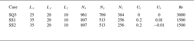

 (a)
 (b)
 dEV/dt
 −Ω/Re
 F
 P

 (a)
 (b)

 (a,b)
 t=0
 (c,d)
 t=52.5
 (e,f)
 t=65
 (g,h)
 t=85

 (a)
 d
 (b)
 xr
 t=61
 t=61.5

 (a)
 Ω
 (b)
 Ωmax
 Ωmax
 t=65
 t=65.5

 (a)
 t=45
 (b)
 t=65.5
 (c)
 t=72
 (d)
 t=10
 (e)
 t=17
 (f)
 t=25

 (a,b)
 t=10
 (c,d)
 t=19
 (e,f)
 t=22
 (g,h)
 t=28
 (i,j)
 t=35
 t=35


 Open access

