1. Introduction
Industrial robots are widely used in welding, spraying, handling, and automated production lines due to their stability, rapid movement, low cost, and ability to operate in environments unsafe for humans [Reference Pham and Ahn1]. In recent years, advances in additive manufacturing and robotics have spurred their adoption across various industries, fundamentally reshaping product manufacturing. The combination of these technologies enables multi-axis additive manufacturing and the fabrication of complex geometries. A significant limitation of traditional additive manufacturing systems, such as the three-axis gantry system used for layer-by-layer printing, is their constrained working envelope [Reference Li, Haghighi and Yang2, Reference Zhao, Ma, Xiao and Tian3]. In contrast, industrial robots perform printing within large workspace areas. Although robotic systems may sacrifice some accuracy compared to three-axis systems, they are ideal for manufacturing large parts and integrating multiple techniques in a single workspace [Reference Bandari, Ding, Bandari, Williams and Martina4].
The RAMLAB laboratory at the Port of Rotterdam, Netherlands, combined arc additive manufacturing and subtractive manufacturing to print a marine propeller with a diameter of 1.3 m and a mass of 400 kg [Reference Dai, Feng, Xu, Huang, He and Shi5]. Song et al. [Reference Song, Yang, Guo, Cui and Yan6] developed a mobile manipulator platform for concrete 3D printing that manufactures products through layer-by-layer deposition. Poudel et al. [Reference Poudel, Marques, Williams, Hyden, Guerra, Fowler, Sha and Zhou7] introduced cooperative 3D printing, a concept wherein multiple mobile 3D printing robots collaborate to produce a single part. However, the aforementioned industrial robots in Fused Deposition Modeling (FDM) additive manufacturing are typically employed either for applications with relatively low precision requirements or in hybrid manufacturing systems that combine additive and subtractive processes.
The quality of final products in additive manufacturing is primarily related to the machine accuracy. Several factors influence the accuracy of additive manufacturing, including (1) robot motion accuracy, which is affected by kinematic model errors and nozzle calibration. (2) The non-parametric nature of the additive manufacturing path, which consists of continuous short line segments and tens of thousands of path points. (3) The high nonlinear dynamic model and uncertainties cause difficulties in designing high-performance controllers. (4) Additive manufacturing process parameters, such as processing technology and environmental control. (5) Mechanical performance of robot equipment. This paper mainly addresses the first three factors.
To address these challenges, several research efforts have focused on accuracy control through both offline and online compensation methods. Offline compensation typically involves identifying parameters [Reference Wang, Xie, Jiang, He and Chen8, Reference Luo, Gao, Huang and Zhang9] and modeling error sources [Reference Shen, Tang, Ye and Zhang10, Reference Ojer, Etxezarreta, Kortaberria, Ahmed, Flores, Hernandez, Lazkano and Lin11]. Online compensation methods, utilizing external measuring and sensing equipment for feedback, are more commonly employed. These methods include secondary grating feedback for joint space [Reference Uhlmann, Polte and Blumberg12, Reference Li, Tian, Li and Zhang13] and visual servoing feedback for Cartesian space [Reference Maghami and Khoshdarregi14, Reference Li, Li, Tian and Liao15]. It is worth noting that the secondary grating feedback, as a semi-closed-loop method, requires modifications and installation of a grating scale. In contrast, visual feedback provides direct measurements of the end-effector’s position and orientation, which represents a fully closed-loop approach. Zhao et al. [Reference Zhao, Lin, Xi, Guo and Ouyang16] designed the robotic riveting system with visual servoing and proposed a control scheme with varying parameter-linear sliding surfaces and second-order sliding surfaces to ensure accurate rivet positioning and robust path-following. Shu et al. [Reference Shu, Gharaaty, Xie, Joubair and Bonev17] introduced a dynamic path-tracking method for industrial robots based on position visual servoing and an adaptive Kalman filter, improving tracking accuracy to
 $\pm 0.2$
mm. Li et al. [Reference Li, Cui, Lin and Zheng18] proposed an attitude measurement method for robot end-effectors using inertial technology with the fourth-order Runge-Kutta algorithm, achieving an attitude accuracy reach 0.15
 $^{\circ }$
. In visual system processing, Ma et al. [Reference Ma, Zhu, Li, Zheng, Zhou, Wang and Wai Samuel Au19] developed a calibration method for vision system parameters, employing a minimal depth-dependent distortion model to reduce lens distortion and enhance measurement precision. Jiang et al. [Reference Jiang, Deng, Yin, Yang, Wang and Zhou20] focused on calibrating the coordinate system within the binocular vision field, creating a method that combines both global and local vision systems for transformation matrix calibration.
Current research on visual servoing mainly focuses on simple straight or arc trajectories. However, additive manufacturing paths, typically generated by Computer-Aided Manufacturing (CAM) software, are composed of numerous short linear segments, making it difficult to define trajectories mathematically. It becomes challenging to obtain accurate target points in robot motion control, and pauses at corners affect the effectiveness of visual servoing. Overfill and underfill of material at the corners negatively impact the geometrical quality of products manufactured by FDM 3D printing. Ref. [Reference Jiang and Ma21] indicates that the printing path influences the shape accuracy of printed parts directly. To alleviate this issue, the implementation of corner smoothing for the trajectory is deemed essential.
To achieve corner smoothness in continuous linear paths, transition methods known as corner smooth methods are proposed, which typically utilize parametric curves of circular arcs to blend adjacent linear segments [Reference Zhao, Zhu and Ding22, Reference He, Fang, Bao, Yang and Zhang23]. Zhang et al. [Reference Zhang, Liu, Yan, Bi and Han24] introduced a real-time look-ahead algorithm to improve precision and minimize damage. The path-smoothing method inserts a quintic Bezier curve between small adjacent line segments to achieve
 $G^2$
continuity at junctions. To achieve better shape accuracy in 3D printing, Communal et al. [Reference Comminal, Serdeczny, Pedersen and Spangenberg25] developed a path-planning strategy that considers the shape accuracy of the corners in each layer of additive manufacturing. Liu et al. [Reference Liu, Zhao, Li, Liu, Wang and Yue26] proposed a composite path planning method that incorporates a sharp corner correction strategy to improve the shape accuracy of parts. Zapata et al. [Reference Zapata, Bendo, Spreitler, Zhao, Bernauer, Yoshioka and Zaeh27] introduced a pixel-based model predicting overfill based on trajectory and traverse speed, controlling wire speed to mitigate corner overflow. Nevertheless, these methods have been primarily studied in machine tools, with fewer studies focusing on the integration into robotic systems. Zhu et al. [Reference Zhu, He, Yu and Li28] proposed a smooth trajectory-planning method combining Cartesian and joint space (using a fifth-order B-spline curve in joint space) to enhance smoothness and reduce vibrations. However, this planning may lead to deviations from the original Cartesian trajectory, which is not permitted in additive manufacturing.
The research outlined above has made notable contributions in the areas of robot motion tracking compensation and trajectory planning. However, there remains an urgent need to further enhance accuracy, particularly for intricate paths in robotic additive manufacturing. This paper aims to build on prior work by designing a generalized non-parametric trajectory planning method that integrates corner-smoothing and real-time interpolation in parallel. By applying chord error and speed continuity as constraints, the proposed method reduces corner overflow and enhances shape accuracy in additive manufacturing. Additionally, the paper introduces a novel robot error compensation controller that combines RBF neural network-based dynamic feedforward control with visual servoing-based feedback control. The controller incorporates variable gain parameters to adapt to speed variations in the additive manufacturing process, along with a velocity observer to reduce measurement noise, enhancing the robot’s dynamic response and trajectory tracking accuracy. Contributions of this paper are summarized as follows.
-
(1) A generalized non-parametric trajectory planning method is developed, integrating chord error and speed continuity as constraints. By combining the dynamic look-ahead planning with real-time interpolation in a parallel structure, it ensures smooth trajectory transitions and speed continuity, effectively balancing precision and quality.
-
(2) An error control method based on visual servoing feedback and RBF neural networks dynamic feedforward is proposed. This method enables the online prediction of dynamic parameters and employs a variable gain controller to address frequent velocity changes in the continuous short-line trajectory of the additive manufacturing process, significantly enhancing the trajectory accuracy of the robot.
-
(3) An open and compatible robotic additive manufacturing platform is developed to address challenges in system integration. The host computer is responsible for NC code parsing, task scheduling, high-level command generation, and non-real-time state monitoring. The PLC-based real-time controller handles low-level motion control, including dynamics modeling, trajectory interpolation, and real-time execution of control algorithms. All components are integrated into one system, facilitating a collaborative system and providing a new solution for robotic manufacturing system integration.
The remainder of this paper is structured as follows. Section 2 introduces the primary methods. Section 3 discusses the experiments and results. The conclusion is provided in Section 4.
2. Methods for trajectory planning and tracking control
2.1. Establishment of the workspace frame
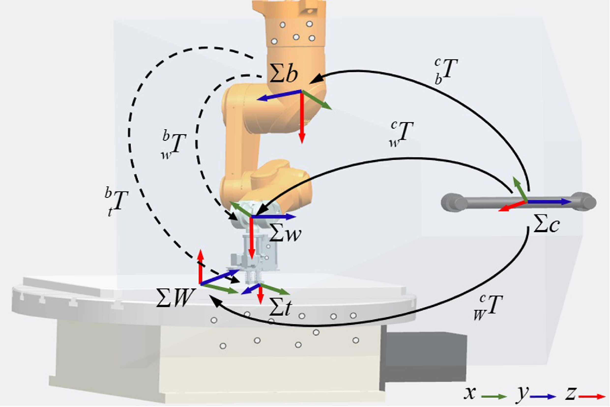
As illustrated in Figure 1, a robotic additive manufacturing system is proposed, consisting of an industrial robot equipped with a printing end-effector, a rotating platform, and a binocular vision instrument (BVI). The robot is installed upside down on the gantry for additive manufacturing. Within the BVI coordinate system, the camera frame
 $\Sigma c$
is defined with its origin located at the midpoint between the two cameras and the z-axis aligned with the optical axis of the cameras. The coordinate frames of the robot base (
 $\Sigma b$
), robot wrist (
 $\Sigma w$
), and turning platform (
 $\Sigma W$
) are also established within the BVI software environment. The tool frame
 $\Sigma t$
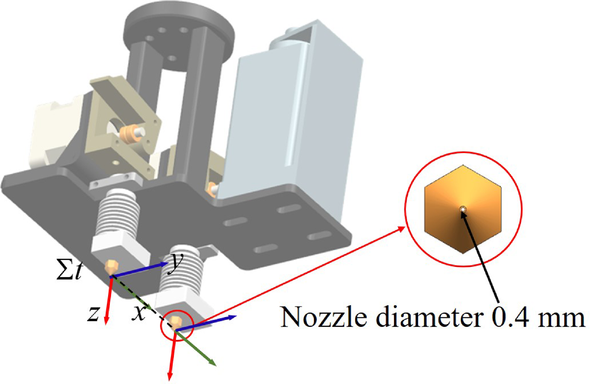
is defined such that the x-axis is aligned with the direction connecting the two nozzles, and the z-axis is aligned with the wrist frame; the y-axis is determined by the right-hand rule. The relationship between the tool frame
 $\Sigma t$
on the end-effector and the wrist frame
 $\Sigma w$
can be obtained, as shown in Figure 2. The reflectors are mounted on the robot base, end-effector, and turntable, respectively, and are tracked by the BVI system. As a position-based visual feedback device, the BVI provides real-time pose information of the tracked objects using three or more non-collinear feature points. It is important to note that during any movement, all corresponding frames must remain within the field of view of the BVI.
Robotic additive manufacturing system and space transformation of each frame.
Schematic diagram of the tool frame.
Using VXelements software and the BVI (C-track 780) from Creamform, the positional and rotational information of the tracked model relative to the camera frame
 $\Sigma c$
can be acquired, recorded, and displayed simultaneously. Therefore, the homogeneous transform matrix
 ${}_b^c{\boldsymbol{T}}$
from
 $\Sigma b$
to
 $\Sigma c$
,
 ${}_w^c{\boldsymbol{T}}$
from
 $\Sigma w$
to
 $\Sigma c$
, and
 ${}_W^c{\boldsymbol{T}}$
from
 $\Sigma W$
to
 $\Sigma c$
can be obtained at any time. The homogeneous transformation matrix
 ${}_w^b{\boldsymbol{T}}$
,
 ${}_W^b{\boldsymbol{T}}$
and
 ${}_w^W{\boldsymbol{T}}$
can be obtained as follows
 \begin{align} {}_w^b{\boldsymbol{T}} &= {}_c^b{\boldsymbol{T}}{}_w^c{\boldsymbol{T}} = {({}_b^c{\boldsymbol{T}})^{ - 1}}{}_w^c{\boldsymbol{T}} \nonumber\\[4pt]{}_W^b{\boldsymbol{T}} &= {}_c^b{\boldsymbol{T}}{}_W^c{\boldsymbol{T}} = {({}_b^c{\boldsymbol{T}})^{ - 1}}{}_W^c{\boldsymbol{T}}\\[4pt]{}_w^W{\boldsymbol{T}} & = {}_c^W{\boldsymbol{T}}{}_w^c{\boldsymbol{T}} = {({}_W^c{\boldsymbol{T}})^{ - 1}}{}_w^c{\boldsymbol{T}}\nonumber \end{align}
Suppose
 $n$
feature points on the rigid end-effector are fixed and known from the definition of the tool frame
 $\Sigma w$
, whose homogeneous coordinates
 $ {}^w \boldsymbol{P}_i = \left[ \begin{array}{l@{\quad}l@{\quad}l@{\quad}l} {}^w{x_i}&{}^w{y_i}&{}^w{z_i}&1 \end{array} \right ]$
are denoted. With the pose
 $({x_t},{y_t},{z_t},{\alpha _t},{\beta _t},{\gamma _t})$
of
 $\Sigma w$
in
 $\Sigma c$
, the homogeneous transformation matrix
 ${}_w^c{\boldsymbol{T}}$
can be formulated as follows
 \begin{equation} { {}_w^c{\boldsymbol{T}} = \left [ {\begin{array}{c@{\quad}c} {R({\alpha _t},{\beta _t},{\gamma _t})}&{{{({x_t},{y_t},{z_t})}^T}}\\ 0&1 \end{array}} \right ]=\left [\begin{array}{c@{\quad}c@{\quad}c@{\quad}c} c \alpha _t c \beta _t & c \alpha _t s \beta _t s \gamma _t-s \alpha _t c \gamma _t & c \alpha _t s \beta _t c \gamma _t+s \alpha _t s \gamma _t & x_t \\ s \alpha _t c \beta _t & s \alpha _t s \beta _t s \gamma _t+c \alpha _t c \gamma _t & s \alpha _t s \beta _t c \gamma _t-c \alpha _t s \gamma _t & y_t \\ -s \beta _t & c \beta _t s \gamma _t & c \beta _t c \gamma _t & z_t \\ 0 & 0 & 0 & 1 \end{array}\right ] } \end{equation}
where
 $R({\alpha _t},{\beta _t},{\gamma _t})$
is the rotation matrix from
 $\Sigma w$
in
 $\Sigma c$
and is taken from the ZYX-form Euler angle,
 $s$
and
 $c$
are the abbreviated forms of the functions
 $sin$
and
 $cos$
, respectively. Therefore, for the
 $i$
th feature point, the transformation equation as
 \begin{equation} {}^c{{\boldsymbol{P}}_i} = {}_w^c{\boldsymbol{T}}{}^w{{\boldsymbol{P}}_i} \end{equation}
The pose
 ${}^c{{\boldsymbol{P}}_i}$
of the manipulator can be obtained, with computations carried out in VXelements.
2.2. Trajectory planning algorithm for continuous path
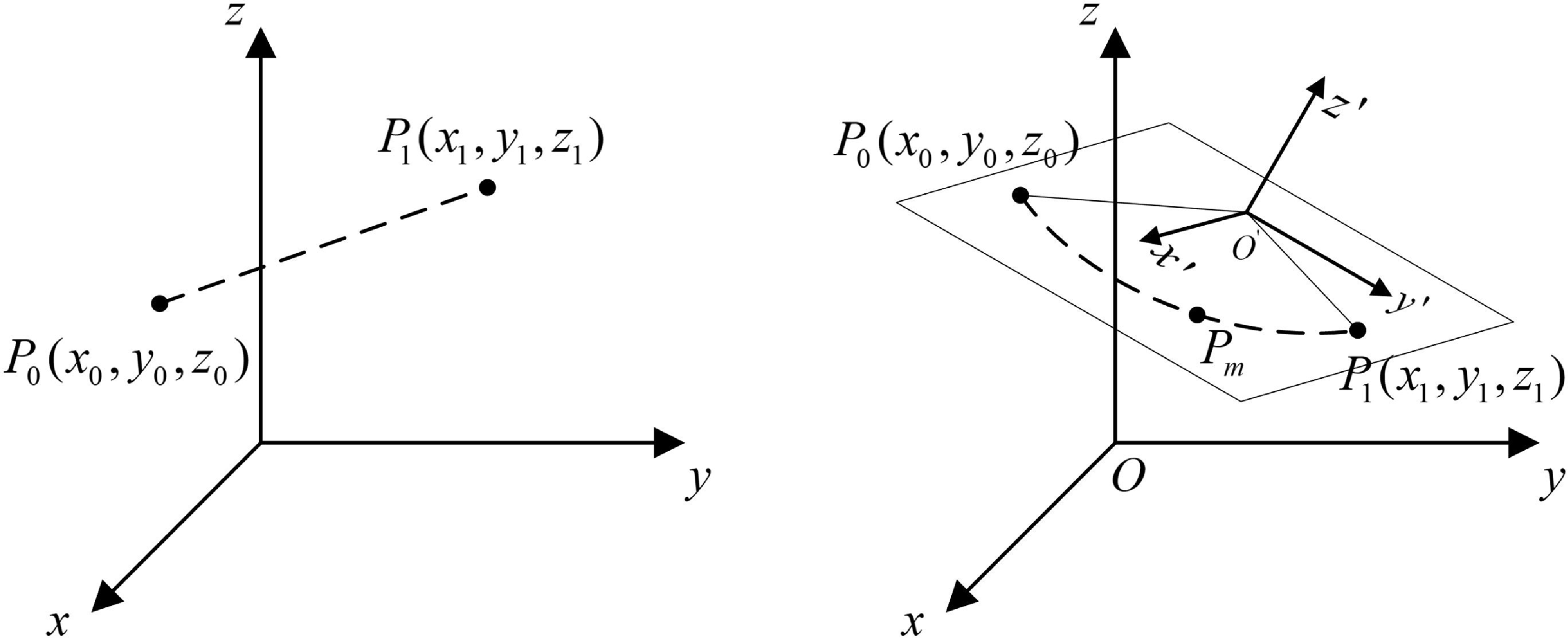
The printing path is determined by the geometric shape of the additive manufacturing part, which consists of contour and infill paths. The slicing software divides the model into layers and generates cross-sectional paths based on the contours. For the printing plane with a spatial or inclined angle, the slicing software generates the infill path by setting the angle between the slicing plane and the printing base plane. A local interpolation frame is established in the slicing plane, and the coordinate transformation relationship between it and the printing base plane is obtained. In the local interpolation frame, the printing path is discretized into a series of planar free-form paths, which consist of straight lines and arcs. Therefore, trajectory interpolation for these straight lines and arcs is a critical aspect of robotic motion. In this paper, the trapezoidal velocity curve interpolation algorithm is employed for linear trajectory planning. This algorithm ensures smooth robotic movement, avoiding sudden speed changes that could cause shaking. For circular arc interpolation, a constant velocity interpolation method is used. Ensuring a smooth transition in velocity between the end of the linear segment and the circular arc. A schematic of linear and circular interpolation is shown in Figure 3.
Diagram of linear and circular interpolation.
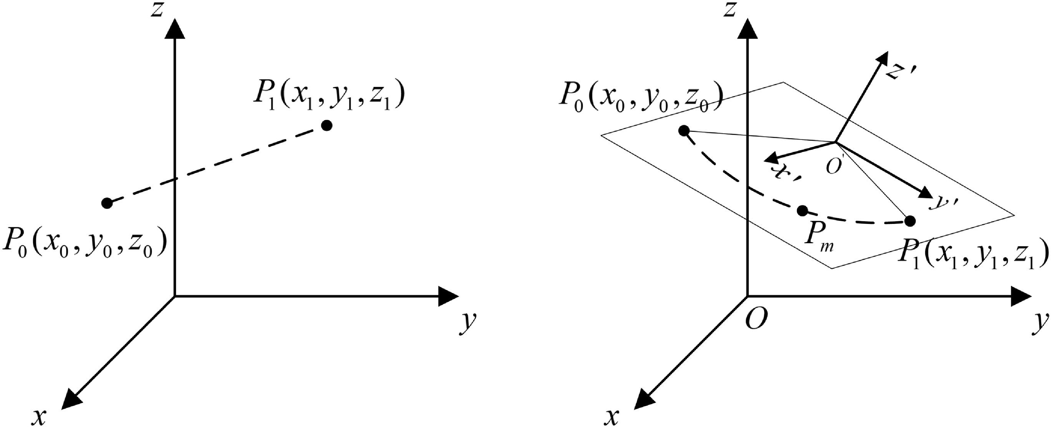
The NC code contains essential information such as robot pose, speed and acceleration limits, nozzle selection, and filament feed rate. When moving in continuous linear no-arc transition mode (the stop-at-turn motion), the robot is required to decelerate to a complete stop before changing direction and then re-accelerate afterward, which significantly increases the printing time [Reference Zhao, Zhu and Ding22]. Meanwhile, due to the filament material overflow caused by the nozzle pressure, the quality of the additive manufacturing products is further compromised when the robot stops at the corner. To enhance the speed continuity and print quality, the trajectory planning method for continuous linear arc transition is proposed. By limiting the maximum normal acceleration of small arcs, the speed at the corners can be restricted, and the accuracy effect is considered. The method results in smaller shape deviations and enables faster printing compared to the continuous linear no-arc transition method, thereby achieving a balance between print quality and manufacturing time.
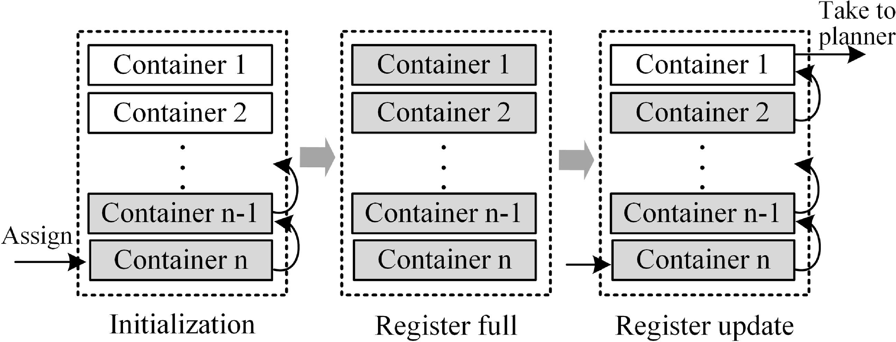
For continuous short straight paths, a register is used to store the path information from the NC code for look-ahead planning, as illustrated in Figure 4. The register is first initialized, and the point data is sequentially stored from the
 $n-th$
container to the first container. The top of the register is then accessed to enable continuous linear arc transition planning, with the container data moving forward sequentially. After completing a segment of continuous path motion, a request is sent to the host computer system to retrieve a new set of data, thereby facilitating the update to the register.
The design for the register.
Continuous linear corners with arc transition.
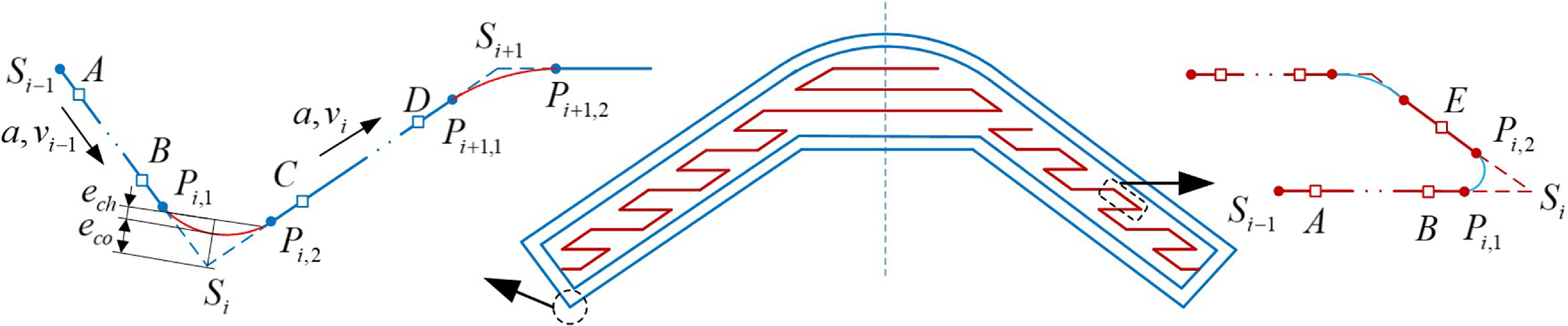
For trajectory planning around corners, the robot’s velocity must transition smoothly at corner points to minimize speed fluctuations and improve motion stability. As discussed in Ref. [Reference Liu, Zhao, Li, Liu, Wang and Yue26], adjusting the robot’s speed to maintain continuity and smoothness through arc corners minimizes overflow and improves part quality. As shown in Figure 5, the additive manufacturing path employs smooth transitions using arcs, where the distance between the arc and the corner point is defined as the contour error
 $e_{co}$
. The deviation between the actual and the theoretical chord is termed the chord error
 $e_{ch}$
. Both errors are kept within acceptable limits. At the initial transition radius of the path at the
 $i-th$
corner point and the
 $(i+1)-th$
corner point, the radius is defined as follows
 \begin{equation} \begin{aligned} & r_i=\sin (\theta _i / 2) \cdot (e_{c o}-e_{c h}) / (1-\sin (\theta _i / 2)) \\ & r_{i+1}=\sin (\theta _{i+1} / 2) \cdot (e_{c o}-e_{c h}) / (1-\sin (\theta _{i+1} / 2)) \end{aligned} \end{equation}
where
 $\theta _i$
represents the angle between the two lines at the
 $i-th$
corner point. The projection lengths of the two arc segments on
 $\overrightarrow {{S_{i}}{S_{i+1}}}$
are
 \begin{equation} \begin{aligned} & L_{S_i P_{i,2}}=r_i / \tan (\theta _i / 2) \\ & L_{S_{i+1} P_{(i+1),1}}=r_{i+1} / \tan (\theta _{i+1} / 2) \end{aligned} \end{equation}
If
 $L_{S_i S_{i+1}}\lt L_{S_i P_{i,2}}+L_{S_{i+1} P_{(i+1),1}}$
the midpoint constraint method is required for initial adjustment.
 \begin{equation} \left \{\begin{array}{c} L_{S_i P_{i, 2}}=L_{S_i S_{i+1}}-L_{S_{i+1} P_{(i+1), 1}}, \min \left \{L_{S_i P_{i, 2}}, L_{S_{i+1} P_{(i+1), 1}}\right \}\lt 0.5 \times L_{S_i S_{i+1}} \cap L_{S_i P_{i, 2}}\gt L_{S_{i+1} P_{(i+1), 1}} \\ L_{S_{i+1} P_{i(i-1), 1}}=L_{S_i S_{i+1}}-L_{S_i P_{i, 2}}, \min \left \{L_{S_i P_{i, 2}}, L_{S_{i-1} P_{i(i+1), 1}}\right \}\lt 0.5 \times L_{S_i S_{i+1}} \cap L_{S_{i+1} P_{(i+1), 1}}\gt L_{S_i P_{i, 2}} \\ L_{S_i P_{i, 2}}=L_{S_{i+1} P_{i(i+1), 1}}=0.5 \times L_{S_i S_{i+1}}, \min \left \{L_{S_i P_{i, 2}}, L_{S_{i+1} P_{(i+1) 1}}\right \} \geq 0.5 \times L_{S_i S_{i+1}} \end{array}\right . \end{equation}
The corrected radius of the arc is given by
 \begin{equation} \begin{aligned} & r_i=L_{S_i P_{i,2}} \cdot \tan (\theta _i / 2) \\ & r_{i+1}=L_{S_{i+1} P_{(i+1), 1}} \cdot \tan (\theta _{i+1} / 2) \end{aligned} \end{equation}
The kinematic constraint for the motion along the arc segment is
 $v_{i c}^2=a \times r_i$
. However, the actual arc velocity is determined by the minimum value among the maximum allowable velocity, the maximum velocity under the chord error constraint, and the system’s rated maximum velocity, which is given by
 \begin{equation} v_c=\min (v_{i c}, v_{e_{-} c h}, v) \end{equation}
where
 $v_{e_{-} c h}=2 / t \times \sqrt {2 r \times e_{c h}-e_{c h}^2}$
,
 $t$
is interpolation period.
Furthermore, it is necessary to determine whether the linear trajectory can meet the velocity conditions. Specifically, this involves verifying whether the endpoint velocity of the previous arc can accelerate or decelerate to the starting velocity of the next arc. If this is not feasible, adjustments are made by fixing the arc radius and corner velocity on one side while modifying the arc radius and velocity on the other side, in conjunction with the velocity planning of the straight-line segment.
The detailed trajectory planning process is described as follows.
 $S_i$
represent the feature points in the toolpath trajectory, which are obtained from the NC code. A sharp corner is defined by two successive linear segments
 $\overrightarrow {{S_{i-1}}{S_{i}}}$
and
 $\overrightarrow {{S_{i}}{S_{i+1}}}$
of the toolpath,
 $a$
and
 $v$
represent the acceleration or deceleration and maximum speed, respectively. The small square points
 $A$
,
 $B$
,
 $C$
, and
 $D$
represent the speed change points. The robot trajectory typically follows a four-step velocity profile:
-
• 1. Acceleration phase to reach the maximum target cruising speed, along the segment line
 $S_iA$
,
-
• 2. Uniform speed phase at constant speed
$v_{i}$
, along the segment line
$AB$
, -
• 3. Deceleration phase while approaching the arc corner, along the segment line
$BP_{i,1}$
, -
• 4. Uniform speed phase, along the curve
$P_{i,1}P_{i,2}$
.


Next, repeating the aforementioned steps. It is important to emphasize that if a line segment is short enough, it may bypass step 2, undergoing acceleration and direct deceleration. For example, the point
 $E$
on the right of Figure 5 serves as the transition point between acceleration and direct deceleration.
In the linear interpolation, let
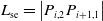 $L_{\mathrm{se}}=\left |P_{i, 2} P_{i+1,1}\right |$
be the length of the line segment,
 $v_s$
be the starting velocity, and
 $v_e$
be the ending velocity of the line segment,
 $v_{max}=v_i$
. If
 $L_{\mathrm{se}}\lt \left |\left (v_s^2-v_{\mathrm{e}}^2\right )\right | /(2a)$
, and
 $L_{\mathrm{se}}\lt \left |\left (v_s^2-v_{\mathrm{e}}^2\right )\right | /(2 a)$
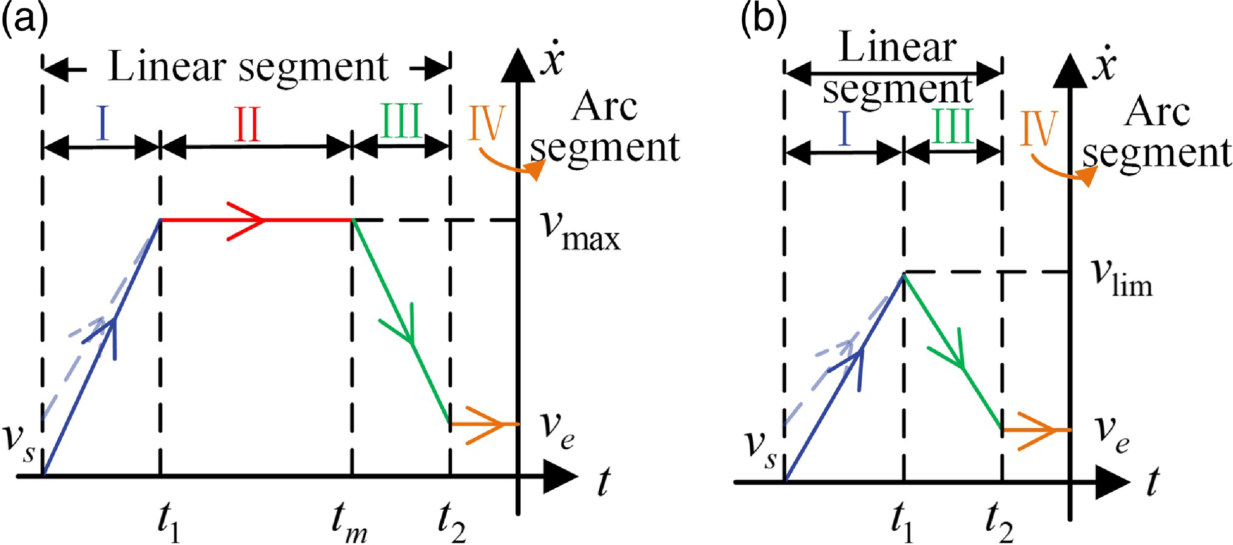
, then there is no constant velocity stage in the trajectory, corresponding to Figure 6(b). The maximum velocity that the trajectory can reach is
 \begin{equation} v_{\lim }=\sqrt {L_{\mathrm{se}} \cdot a+\frac {v_{\mathrm{s}}^2+v_{\mathrm{e}}^2}{2}} \end{equation}
The acceleration duration
 $t_1$
and deceleration duration
 $t_2$
are respectively
 \begin{equation} t_1=\frac {v_{\max }-v_{\mathrm{s}}}{a}, t_2=\frac {v_{\max }-v_{\mathrm{e}}}{a} \end{equation}
The displacement at the interpolation time
 $t$
 \begin{equation} P_l(t)=\left \{\begin{array}{c@{\quad}c} v_s \cdot t+\dfrac {1}{2} a \cdot t^2, & 0 \leq t \leq t_1 \\[5pt] L_1+v_{\lim } \cdot t-\dfrac {1}{2} a \cdot t^2, & t_1\lt t \leq t_1+t_2 \end{array}\right . \end{equation}
where
 $L_1=v_s \cdot t_1+\left (a \cdot t_1^2\right ) / 2$
.
Otherwise, the trajectory includes acceleration, uniform speed, and deceleration stages, corresponding to Figure 6(a). In this case, the acceleration duration
 $t_1$
and deceleration duration
 $t_2$
are respectively
 \begin{equation} t_1=\frac {v_{\max }-v_{\mathrm{s}}}{a}, t_2=\frac {v_{\max }-v_{\mathrm{e}}}{a} \end{equation}
The uniform speed duration is
 \begin{equation} t_{\mathrm{m}}=\frac {L_{\mathrm{se}}-\left (\frac {v_{\max }^2-v_{\mathrm{s}}^2}{2 a}+\frac {v_{\max }^2-v_{\mathrm{e}}^2}{2 a}\right )}{v_{\max }} \end{equation}
The displacement at the interpolation time
 $t$
 \begin{equation} P_l(t)=\left \{\begin{array}{c@{\quad}c} v_s \cdot t+\dfrac {1}{2} a \cdot t^2, & 0 \leq t\lt t_1 \\ L_1+v_{\max } \cdot \left (t-t_1\right ), & t_1 \leq t\lt t_1+t_{\mathrm{m}} \\ L_2+v_{\max } \cdot \left (t-t_2\right )-\dfrac {1}{2} a \cdot \left (t-t_2\right ), & t_1+t_{\mathrm{m}} \leq t \leq t_1+t_2+t_{\mathrm{m}} \end{array}\right . \end{equation}
where
 $L_2=L_1+v_{\max } \cdot t_{\mathrm{m}}$
.
For circular arc interpolation, a uniform speed planning method is employed to derive the expressions of arc length and central angle as functions of time
 \begin{equation} \begin{aligned} &l(t)=v_e \cdot t\\ &\theta (t)=\theta \cdot l(t) / S \end{aligned} \end{equation}
where
 $S$
represents the arc length,
 $\theta$
denotes the central angle corresponding to the arc length. The interpolation points in the local coordinate system are expressed as a function of time
 \begin{equation} P_c(t)=[R \cdot \cos (\theta (t)), R \cdot \sin (\theta (t))] \end{equation}
Finally, the interpolation points are transformed from the local coordinate system to the printing base plane by the transformation matrix
 $_b^l T$
, yielding the interpolation points in the printing base plane is
 \begin{equation} \left \{\begin{array}{l} P(t)={ }_b^l T \cdot P_l(t) \text{ for line } \\ P(t)={ }_b^l T \cdot P_c(t) \text{ for arc } \end{array}\right . \end{equation}
Schematic diagram of the phase trajectory: (a) Long-distance positioning; (b) Short-distance positioning.
Setting the velocity of the filament feeding motor to match the velocity of the robot’s end-effector, the velocity of the filament feeding motor
 $v_{fm}$
is
 \begin{equation} v_{f m}=\frac {v_a}{v} \cdot v_m \end{equation}
where
 $v$
is the maximum velocity for the robot in the NC code,
 $v_a$
is the actual speed of the robot’s end-effector, and
 $v_m$
is the rated speed of the feeding motor in the robot’s maximal motion velocity.
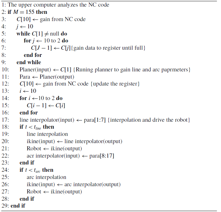
The execution logic of the planning algorithm is illustrated in Figure 7, encompassing NC code parsing, register storage, trajectory planning, and cross-interpolation of linear and circular trajectories. The sequential execution is indicated by the black arrow line, while parallel execution is represented by the red and green arrows. Notably, the red line signifies the arc interpolation input assignment, and the subsequent trajectory planning is executed in parallel with linear interpolation. The green line denotes the linear interpolation input assignment and the arc interpolation in parallel. Linear and arc interpolation are executed alternately. The pseudo-code for continuous linear arc transition is provided in Algorithm 1.
Control flow chart for execution logic.
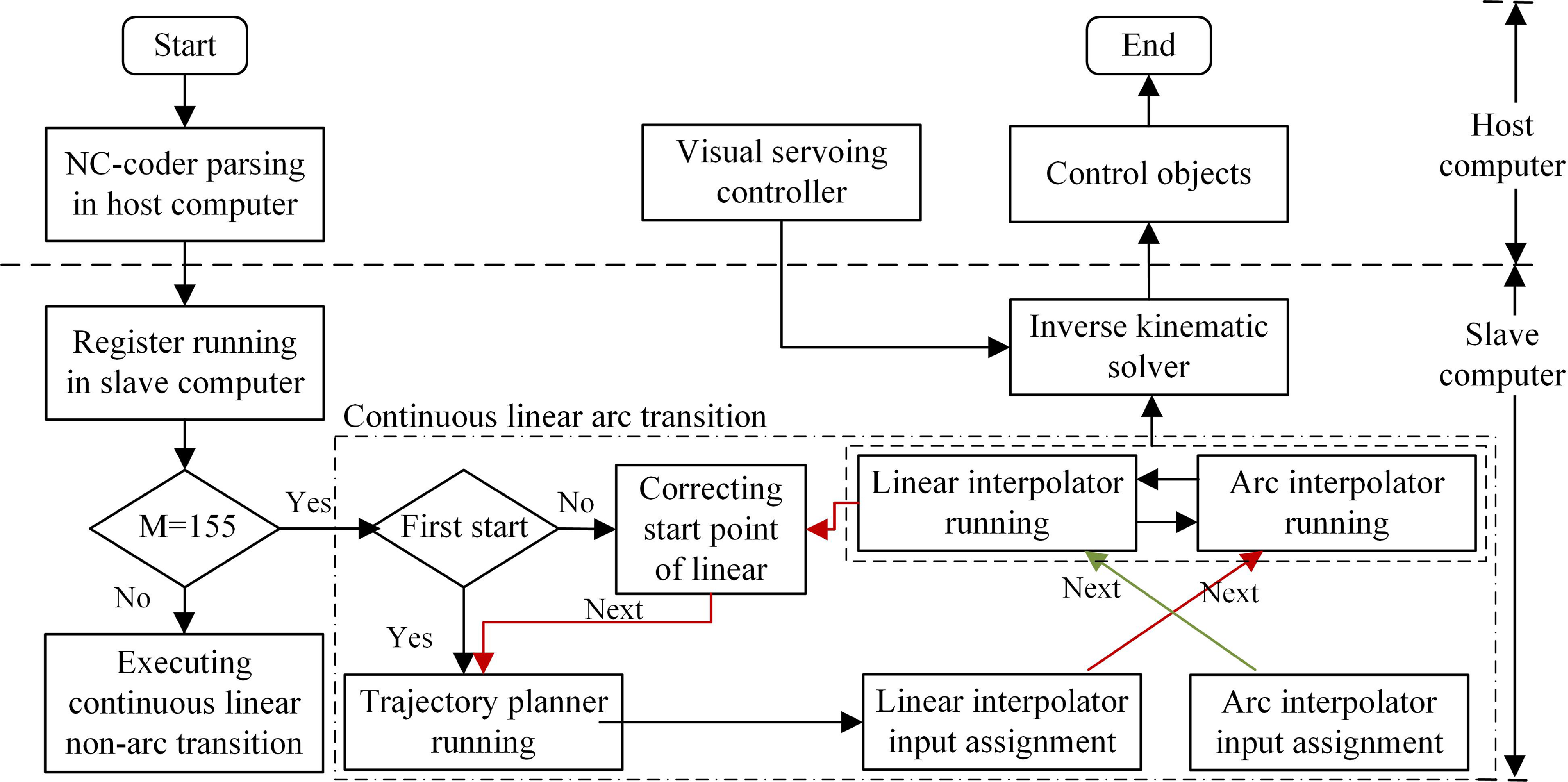
Continuous linear arc transition mode based on the register, the planner, the interpolator, and then drive the robot.
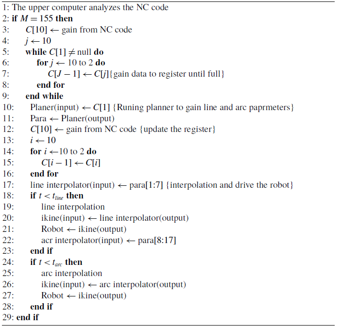
In this algorithm, “M = 155” represents the continuous linear arc transition mode,
 $\boldsymbol{C}$
represents the register container (capacity of 10), and “planner (input)” and “planner (output)” represent inputs and outputs of the trajectory planner module, respectively. Similarly, the “ikine,” “line interpolator,” and “arc interpolator” represent the inverse kinematic solver, linear interpolator module, and circular interpolator module, respectively. The “para” represents an array of capacity 17 used to temporarily store the output of the planner. The “para [1:7]” represents the motion parameters of a line segment (start/end point coordinates and velocity), while the “para [8:17]” represents the motion parameters of an arc segment (start/mid/end point coordinates and velocity).
 $t_{line}$
and
 $t_{arc}$
represent the time of linear and circular interpolation.
2.3. Tracking control based on visual servoing
In the robotic operational space, the Cartesian-space vector
 $\boldsymbol{x}$
is defined as the position and orientation of the end-effector. According to the robot kinematic, the vector
 $\boldsymbol{x}$
is dependent on the joint configuration and can be expressed as a function of joint-space displacements as
 \begin{equation} {\boldsymbol{x}} = {\boldsymbol{h}}({\boldsymbol{q}}) \end{equation}
where
 ${\boldsymbol{h}}({\bullet})$
represents a nonlinear function that computes the operational space position variables from the joint space position variables.
 $\dot{\boldsymbol{x}}$
denotes a velocity vector in Cartesian space, which is related to the joint-space velocity vector
 $\dot{\boldsymbol{q}}$
by
 \begin{equation} {\dot{\boldsymbol{x}}} = {{\boldsymbol{J}}_m}({\boldsymbol{q}}){\dot{\boldsymbol{q}}} \end{equation}
where
 ${{\boldsymbol{J}}_m}({\boldsymbol{q}})$
is the link Jacobian matrix.
Consider a bounded continuous trajectory, which is designed far away enough from any singularity. In the joint space, the dynamics of a serial n-link rigid robot can be written as
 \begin{equation} \boldsymbol{M}(\boldsymbol{q})\ddot{\boldsymbol{q}} + \boldsymbol{C}(\boldsymbol{q,}\, \dot{\boldsymbol{q}})\dot{\boldsymbol{q}} + \boldsymbol{G}(\boldsymbol{q}) = \boldsymbol{\tau } \end{equation}
where
 $\boldsymbol{M(q)} \in \mathbb{R} {^{6 \times 6}}$
denotes the positive definite inertia matrix,
 $\boldsymbol{C}\boldsymbol{(}\boldsymbol{q,}\,\dot{\boldsymbol{q}}\boldsymbol{)} \in \mathbb{R} {^{6 \times 6}}$
is the centrifugal force and Coriolis force term,
 $\boldsymbol{G(q)} \in \mathbb{R} {^{6 \times 1}}$
denotes the gravity term matrix, and
 $\boldsymbol{\tau }$
is the joint control torque matrix.
The dynamic system in Cartesian space is the following form
 \begin{equation} {\boldsymbol{M}_x}(\boldsymbol{q})\ddot{\boldsymbol{x}} + {\boldsymbol{C}_x}(\boldsymbol{q,}\, \dot{\boldsymbol{q}})\dot{\boldsymbol{x}} + {\boldsymbol{G}_x}(\boldsymbol{q}) = {\boldsymbol{F}_x} \end{equation}
where
 ${{\boldsymbol{M}}_x}({\boldsymbol{q}}) = {\boldsymbol{J}}_m^{ - T}({\boldsymbol{q}}){\boldsymbol{M}}({\boldsymbol{q}}){\boldsymbol{J}}_m^{ - 1}({\boldsymbol{q}})$
,
 ${{\boldsymbol{C}}_x}({\boldsymbol{q}}) = {\boldsymbol{J}}_m^{ - T}({\boldsymbol{q}}){\boldsymbol{C}}({\boldsymbol{q}}){\boldsymbol{J}}_m^{ - 1}({\boldsymbol{q}})$
,
 ${{\boldsymbol{G}}_x}({\boldsymbol{q}}) = {\boldsymbol{J}}_m^{ - T}({\boldsymbol{q}}){\boldsymbol{G}}({\boldsymbol{q}})$
,
 ${{\boldsymbol{F}}_x} = {\boldsymbol{J}}_m^{ - T}({\boldsymbol{q}})\boldsymbol{\tau }$
.
 $\textit {Property 1}$
: The centripetal-Coriolis matrix
 ${{\boldsymbol{C}}_x}({\boldsymbol{q}},{\dot{\boldsymbol{q}}})$
possesses the following property:
 ${{\boldsymbol{x}}^T}(\dot{\boldsymbol{M}}_x({\boldsymbol{q}}) - 2{{\boldsymbol{C}}_x}({\boldsymbol{q}},{\dot{\boldsymbol{q}}})){\boldsymbol{x}} = 0$
.
To meet the high precision requirements of additive manufacturing, it is necessary to compensate for the inherent inaccuracies of the robotic system. A visual servoing compensation strategy is established using the BVI, with measurements converted into pose information relative to the robot base frame. Feedback signals are returned to the servo compensation controller, which generates control commands to drive the robot, thereby adjusting its pose and achieving the desired position.
In the working space,
 $\boldsymbol{x}_d$
is the desired position in the desired trajectory, and
 $\dot {\boldsymbol{x}}_d$
and
 ${\ddot{\boldsymbol{x}}}_d$
represent the desired velocity and acceleration, respectively. Define the following equation
 \begin{equation} \begin{array}{l} \Delta {\boldsymbol{x}} = {{\boldsymbol{x}}_d} - {\boldsymbol{x}}\\ {{{\dot{\boldsymbol{x}}}}_r} = {{{\dot{\boldsymbol{x}}}}_d} - \textrm {T}\Delta {\boldsymbol{x}}\\ {\boldsymbol{r}} = {{{\dot{\boldsymbol{x}}}}_r} - {\dot{\boldsymbol{x}}} = \Delta {\dot{\boldsymbol{x}}} + \textrm { T}\Delta {\boldsymbol{x}} \end{array} \end{equation}
where,
 $\Delta {\boldsymbol{x}}$
is the pose error in Cartesian space, and
 $\boldsymbol{x}_d$
and
 $\dot {\boldsymbol{x}}_d$
are obtained by the interpolation module. In the Cartesian-space controller, the Cartesian-space feedback
 $\boldsymbol{x}$
and
 $\dot {\boldsymbol{x}}$
are usually measured by the BVI, which undergoes image processing, filtering, and coordinate transformation. However, due to the presence of measurement noise, directly differentiating position values
 $\boldsymbol{x}$
results in significant errors in velocity
 $\dot {\boldsymbol{x}}$
. To mitigate this issue, a velocity observer is introduced to estimate velocity using measured position data.
 $\mathrm{T}$
is a positive definite matrix.
The dynamic parameters were predicted using the RBF neural networks. The controller in Cartesian space is designed as
 \begin{equation} {{\boldsymbol{F}}_x} = \hat{\boldsymbol{w}}_M^T \cdot {{\boldsymbol{h}}_M}({\boldsymbol{q}}){{\ddot{\boldsymbol{x}}}_r} + \hat{\boldsymbol{w}}_C^T \cdot {{\boldsymbol{h}}_C}({\boldsymbol{z}}){{\dot{\boldsymbol{x}}}_r} + \hat{\boldsymbol{w}}_G^T \cdot {{\boldsymbol{h}}_G}({\boldsymbol{q}}) + {\boldsymbol{Kr}} + {k_s}\mathop {\textrm {sgn}} ({\boldsymbol{r}}) \end{equation}
where
 $(\hat{\bullet})$
is the estimation of
 $({\bullet})$
, the first three terms of the control law are model-based control components predicted by the RBF neural networks, and the construction process is detailed in Appendix A. The
 $\boldsymbol{Kr}$
is the proportional derivative (PD) control term,
 ${{\boldsymbol{K}}_p} = {\boldsymbol{K}}\textrm {T}$
and
 ${{\boldsymbol{K}}_d} = {\boldsymbol{K}}$
are diagonal and positive definite matrices, making
 ${\textrm {T}_{ij}} = \frac {1}{{{K_{ij}}^2}}(i = j)$
. The last term is a robust term to suppress the neural networks’ modeling errors, and
 ${k_s} \gt \left \| {\boldsymbol{E}} \right \|$
.
The control parameters
 $\boldsymbol{K}$
corresponding to the four stages in Figure 6 are designed as
 \begin{equation} \left \{ {\begin{array}{l} {{{\boldsymbol{K}}_{\boldsymbol{I}}} = {\bar{\boldsymbol{K}}} - \dfrac {1}{{2{a_1}}}\Delta {\boldsymbol{x}} \cdot {\boldsymbol{I}}}\\ {{{\boldsymbol{K}}_{\boldsymbol{II}}} = {\bar{\boldsymbol{K}}}}\\ {{{\boldsymbol{K}}_{\boldsymbol{III}}} = {\bar{\boldsymbol{K}}} + \dfrac {1}{{2{a_2}}}\Delta {\boldsymbol{x}} \cdot {\boldsymbol{I}}}\\ {{{\boldsymbol{K}}_{\boldsymbol{IV}}} = \dfrac {{{\bar{\boldsymbol{K}}}}}{2}} \end{array}} \right . \end{equation}
where
 $\bar{\boldsymbol{K}}$
is the nominal value,
 $a_1$
and
 $a_2$
represent the value of acceleration and deceleration, respectively.
 $\boldsymbol{I}$
represents the unit matrix. In the constant acceleration phase, parameters are designed to achieve a smooth and rapid start of the motor. Once the velocity reaches its maximum, the control parameters constrain the operating speed. During deceleration, the parameters ensure a stable and accurate approach to the target position. For short-distance positioning tasks, the uniform speed phase (step 2) is omitted.
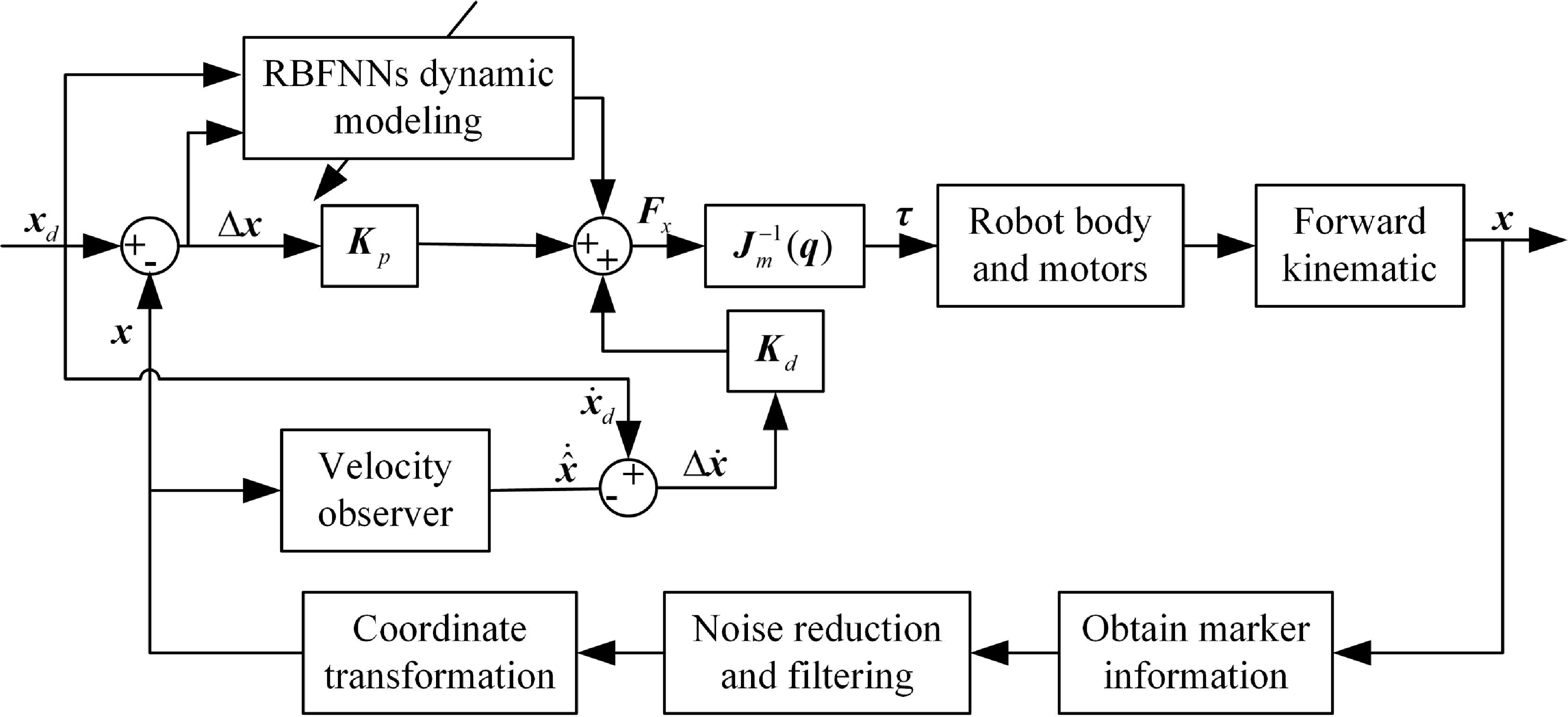
The block diagram of the visual servoing controller integrated with a velocity observer is illustrated in Figure 8. The matrix
 ${{\boldsymbol{J}}_m}({\boldsymbol{q}})$
denotes the Jacobian matrix, and the feedback information in Cartesian space is directly transformed into the controller output of the robot in joint space using the Jacobian matrix.
 $\boldsymbol{\tau }$
is the torque exerted in the joint space.
The principle of the visual servoing controller.
Define the adaptive law of neural networks weights [Reference Wei, Li, Tian, Wei, Bai, Zhang, Li and Hou29]:
 \begin{equation} \begin{array}{l} \dot{\hat{\boldsymbol{W}}}_{Mk} = {{\boldsymbol{\Gamma }}_{Mk}} \cdot {\boldsymbol{\phi } _{Mk}}({\boldsymbol{q}}){{{\ddot{\boldsymbol{x}}}}_r}{{\boldsymbol{r}}_k}\\ \dot{\hat{\boldsymbol{W}}}_{Ck} = {{\boldsymbol{\Gamma }}_{Ck}} \cdot {\boldsymbol{\phi } _{Ck}}({\boldsymbol{z}}){{{\dot{\boldsymbol{x}}}}_r}{{\boldsymbol{r}}_k}\\ \dot{\hat{\boldsymbol{W}}}_{Gk} = {{\boldsymbol{\Gamma }}_{Gk}} \cdot {\boldsymbol{\phi } _{Gk}}({\boldsymbol{q}}){{\boldsymbol{r}}_k} \end{array} \end{equation}
where
 ${\boldsymbol{\Gamma }}_{MK}$
,
 ${\boldsymbol{\Gamma }}_{CK}$
, and
 ${\boldsymbol{\Gamma }}_{GK}$
are the symmetric positive definite matrix, and
 ${\boldsymbol{\phi } _{Mk}}({\boldsymbol{q}})$
,
 ${\boldsymbol{\phi } _{Ck}}({\boldsymbol{z}})$
, and
 ${\boldsymbol{\phi } _{Gk}}({\boldsymbol{q}})$
are the Gaussian kernel functions of the neural networks, respectively.
The velocity observer is proposed to solve the velocity estimation
 \begin{equation} { \begin{array}{l} {\dot {\hat {\boldsymbol{x}}}} = \boldsymbol{P} + \Lambda {\tilde {\boldsymbol{x}}}\\ \dot{\boldsymbol{p}} = \boldsymbol{M}_x^{ - 1}(\boldsymbol{q})[{\boldsymbol{F}_x} - {\boldsymbol{C}_x}(\boldsymbol{q,}\, \dot{\boldsymbol{q}}) \dot {\hat {\boldsymbol{x}}} - {\boldsymbol{G}_x}(\boldsymbol{q})] \end{array} } \end{equation}
where
 $\boldsymbol{p}$
is an auxiliary variable,
 $\Lambda$
is a diagonal positive definite matrix designed based on the stability requirements of the closed-loop system. The expression
 $\Lambda$
will be presented in the stability analysis of the observer system. The dynamic coefficients are parameter values predicted using the RBF neural networks. Note that the equation is basically the robot Eq. (22) with
 $\dot {\boldsymbol{x}}$
replaced by
 $\dot {\hat {\boldsymbol{x}}}$
.
Before the stability of the observer systems is analyzed, the observation error
 $\dot {\tilde {\boldsymbol{x}}}$
for the system is derived. By taking the time derivative of
 $\dot {\hat {\boldsymbol{x}}}$
 \begin{equation} {{\ddot {\hat {\boldsymbol{x}}}}} = \dot {\boldsymbol{p}} + \Lambda {{\dot {\tilde {\boldsymbol{x}}}}} \end{equation}
After pre-multiplying Eq. (28) by
 ${\boldsymbol{M}_x}(\boldsymbol{q})$
, and substituting
 $\dot {\boldsymbol{p}}$
of Eq. (27)
 \begin{equation} {\boldsymbol{M}_x}(\boldsymbol{q}){\ddot {\hat {\boldsymbol{x}}}} = {\boldsymbol{F}_x} - {\boldsymbol{C}_x}(\boldsymbol{q,}\, \dot{\boldsymbol{q}})\dot {\hat {\boldsymbol{x}}} - {\boldsymbol{G}_x}(\boldsymbol{q}) + \Lambda {\boldsymbol{M}_x}(\boldsymbol{q})\dot {\tilde {\boldsymbol{x}}} \end{equation}
Subtracting Eq. (29) from Eq. (22), we obtain the closed-loop error system for Cartesian-space velocity observation error
 $\dot {\tilde {\boldsymbol{x}}}$
as
 \begin{equation} {\boldsymbol{M}_x}(\boldsymbol{q}){\ddot {\tilde {\boldsymbol{x}}}} = - {\boldsymbol{C}_x}(\boldsymbol{q,}\, \dot{\boldsymbol{q}})\dot {\tilde {\boldsymbol{x}}} - \Lambda {\boldsymbol{M}_x}(\boldsymbol{q})\dot {\tilde {\boldsymbol{x}}} \end{equation}
Let the function
 $V_0$
be defined as follows to analyze the velocity observer stability.
 \begin{equation} {V_0} = \frac {1}{2}{{\dot {\tilde {\boldsymbol{x}}}}^T}{{\boldsymbol{M}}_x}({\boldsymbol{q}}){\dot {\tilde {\boldsymbol{x}}}} \end{equation}
Taking the time derivative of
 $V_0$
 \begin{equation} {\dot {V}_0} = {{\dot {\tilde {\boldsymbol{x}}}}^T}{{\boldsymbol{M}}_x}({\boldsymbol{q}}){\ddot {\tilde {\boldsymbol{x}}}} + \frac {1}{2}{{\dot {\tilde {\boldsymbol{x}}}}^T}{{\dot {\boldsymbol{M}}}_x}({\boldsymbol{q}}){\dot {\tilde {\boldsymbol{x}}}} \end{equation}
After substituting the error system for
 $\dot {\tilde {\boldsymbol{x}}}$
of Eq. (30) from Eq. (32), results in
 \begin{equation} \begin{split} {\dot {V}_0} &= \frac {1}{2}{{\dot {\tilde {\boldsymbol{x}}}}^T}{{\dot {\boldsymbol{M}}}_x}({\boldsymbol{q}}){\dot {\tilde {\boldsymbol{x}}}} + {{{\dot {\tilde {\boldsymbol{x}}}}}^T}( - {{\boldsymbol{C}}_x}({\boldsymbol{q}},{\dot{\boldsymbol{q}}}){\dot{\tilde{\boldsymbol{x}}}} - \Lambda {{\boldsymbol{M}}_x}({\boldsymbol{q}}){\dot {\tilde {\boldsymbol{x}}}})\\ &=\frac {1}{2}{{\dot {\tilde {\boldsymbol{x}}}}^T}({{\dot {\boldsymbol{M}}}_x}({\boldsymbol{q}})-2{{\boldsymbol{C}}_x}({\boldsymbol{q}},{\dot{\boldsymbol{q}}})){\dot{\tilde{\boldsymbol{x}}}}-{\dot {\tilde {\boldsymbol{x}}}}^T \Lambda {{\boldsymbol{M}}_x}({\boldsymbol{q}}){\dot {\tilde {\boldsymbol{x}}}} \end{split} \end{equation}
Applying the
 $\textit {property 1}$
, we obtain
 \begin{equation} {\dot {V}_0}=-{\dot {\tilde {\boldsymbol{x}}}}^T \Lambda {{\boldsymbol{M}}_x}({\boldsymbol{q}}){\dot {\tilde {\boldsymbol{x}}}} \le - \Lambda {m_1} \| {\dot {\tilde {\boldsymbol{x}}}} \| \le 0 \end{equation}
 $V_0$
is positive definite,
 $\dot {V_0}$
is semi-negative definite, and the closed-loop system has progressive stabilization. When
 $t \to \infty$
,
 ${\dot {\tilde {\boldsymbol{x}}}} \to \infty$
, the observer serves as an estimator of velocity effectively.
The robot dynamics Eq. (22) is written as Eq. (35) according to Appendix A.
 \begin{equation} \begin{array}{l} {{\boldsymbol{F}}_x} = \left ( {{{\boldsymbol{F}}_{MNN}}({\boldsymbol{q}}) + {{\boldsymbol{E}}_M}} \right ){\ddot{\boldsymbol{x}}} + \left ( {{{\boldsymbol{F}}_{CNN}}({\boldsymbol{z}}) + {{\boldsymbol{E}}_{\boldsymbol{C}}}} \right ){\dot{\boldsymbol{x}}} + \left ( {{{\boldsymbol{F}}_{GNN}}({\boldsymbol{q}}) + {{\boldsymbol{E}}_{\boldsymbol{G}}}} \right ) + {k_s}\mathop {\textrm {sgn}} ({\boldsymbol{r}})\\ = \left [ {{\boldsymbol{w}}_M^T{{\boldsymbol{h}}_M}({\boldsymbol{q}}) + {{\boldsymbol{E}}_M}} \right ]{\ddot{\boldsymbol{x}}} + \left [ {{\boldsymbol{w}}_C^T{{\boldsymbol{h}}_C}({\boldsymbol{z}}) + {{\boldsymbol{E}}_C}} \right ]{\dot{\boldsymbol{x}}} + \left [ {{\boldsymbol{w}}_G^T{{\boldsymbol{h}}_G}({\boldsymbol{q}}) + {{\boldsymbol{E}}_G}} \right ] + {k_s}\mathop {\textrm { sgn}} ({\boldsymbol{r}}) \end{array} \end{equation}
Applying the control law from Eq. (24) to the robot dynamics in Eq. (35) and using Eq.(23) yields the tracking error equation
 \begin{equation} \begin{aligned} & \left [ \boldsymbol{w}_M^T \boldsymbol{h}_M (\boldsymbol{q}) + \boldsymbol{E}_M \right ]{\ddot{\boldsymbol{r}}} + \left [ \boldsymbol{w}_C^T \boldsymbol{h}_C({\boldsymbol{z}}) + \boldsymbol{E}_C \right ]\dot{\boldsymbol{r}}\\ &= {\boldsymbol{M} \dot{\boldsymbol{r}}} + {\boldsymbol{Cr}}= {\tilde {\boldsymbol{w}}}_M^T{{\boldsymbol{h}}_M}({\boldsymbol{q}})\ddot {\boldsymbol{x}}_r + {\tilde {\boldsymbol{w}}}_C^T{{\boldsymbol{h}}_C}({\boldsymbol{z}})\dot {\boldsymbol{x}}_r + {\tilde {\boldsymbol{w}}}_G^T{{\boldsymbol{h}}_G}({\boldsymbol{q}}) + {\boldsymbol{E}} - {\boldsymbol{Kr}} - {k_s}\mathop {\textrm {sgn}} ({\boldsymbol{r}}) \end{aligned} \end{equation}
where
 $(\tilde{\bullet})=({\bullet})-(\hat{\bullet})$
represents the estimation error of the parameter,
 ${\boldsymbol{E}} = {{\boldsymbol{E}}_M}{{\ddot{\boldsymbol{x}}}_r} + {{\boldsymbol{E}}_C}{{\dot{\boldsymbol{x}}}_r} + {{\boldsymbol{E}}_G}$
.
To prove the stability of the system predicted by the RBF neural networks, the Lyapunov function is defined as
 \begin{equation} {V_1} = \frac {1}{2}{{\boldsymbol{r}}^T}{{\boldsymbol{M}}_x}{\boldsymbol{r}} + \frac {1}{2}\sum \limits _{k = 1}^n \tilde{\boldsymbol{w}}_{Mk}^T {\boldsymbol{\Gamma }}_{Mk}^{ - 1}\tilde{\boldsymbol{w}}_{Mk} + \frac {1}{2}\sum \limits _{k = 1}^n \tilde{\boldsymbol{w}}_{Ck}^T {\boldsymbol{\Gamma }}_{Ck}^{ - 1}\tilde{\boldsymbol{w}}_{Ck} + \frac {1}{2}\sum \limits _{k = 1}^n \tilde{\boldsymbol{w}}_{Gk}^T {\boldsymbol{\Gamma }}_{Gk}^{ - 1}\tilde{\boldsymbol{w}}_{Gk} \end{equation}
Computing the derivative of Eq. (37) and simplifying it to get
 \begin{align} \dot{V}_1 = {\boldsymbol{r}}^T \boldsymbol{M} \dot{\boldsymbol{r}} + \frac {1}{2}\boldsymbol{r}^T {\dot{\boldsymbol{Mr}}} + \sum \limits _{k = 1}^n \tilde{\boldsymbol{w}}_{Mk}^T {\boldsymbol{\Gamma }}_{Mk}^{ - 1}\dot{\tilde{\boldsymbol{w}}}_{Mk} + \sum \limits _{k = 1}^n \tilde{\boldsymbol{w}}_{Ck}^T {\boldsymbol{\Gamma }}_{Ck}^{ - 1}{\dot{\tilde{\boldsymbol{w}}}_{Ck}} + \sum \limits _{k = 1}^n \tilde{\boldsymbol{w}}_{Gk}^T {\boldsymbol{\Gamma }}_{Gk}^{ - 1}{\dot{\tilde{\boldsymbol{w}}}}_{Gk} \end{align}
According to
 $\textit {property 1}$
, and
 $ \dot{\tilde{\boldsymbol{w}}}_{MK} = - \dot{\hat{\boldsymbol{w}}}_{Mk}$
,
 $ \dot{\tilde{\boldsymbol{w}}}_{CK} = -{\dot{\hat{\boldsymbol{w}}}}_{Ck}$
,
 $ \dot{\tilde{\boldsymbol{w}}}_{GK} = -\dot{\hat{\boldsymbol{w}}}_{Gk}$
. Substituted into the above formula
 \begin{equation} {\dot V_1} = {{\boldsymbol{r}}^T}(\boldsymbol{M}\dot{\boldsymbol{r}} + {\boldsymbol{Cr}}) - \sum \limits _{k = 1}^n \tilde{\boldsymbol{w}}_{Mk}^T {\boldsymbol{\Gamma }}_{Mk}^{ - 1}{\dot{\hat{\boldsymbol{w}}}}_{Mk} - \sum \limits _{k = 1}^n \tilde{\boldsymbol{w}}_{Ck}^T {\boldsymbol{\Gamma }}_{Ck}^{ - 1}{\dot{\hat{\boldsymbol{w}}}}_{Ck} - \sum \limits _{k = 1}^n \tilde{\boldsymbol{w}}_{Gk}^T {\boldsymbol{\Gamma }}_{Gk}^{ - 1}{\dot{\hat{\boldsymbol{w}}}_{Gk}} \end{equation}
 \begin{equation} \begin{array}{l} {{\dot V}_1} = - {{\boldsymbol{r}}^T}{\boldsymbol{Kr}} + {{\boldsymbol{r}}^T}{\boldsymbol{E}} - {k_s}{{\boldsymbol{r}}^T}\mathop {\textrm {sgn}} ({\boldsymbol{r}}) + {{\boldsymbol{r}}^T}\tilde{\boldsymbol{w}}_M^T \cdot {{\boldsymbol{h}}_M}({\boldsymbol{q}}){{{\ddot{\boldsymbol{x}}}}_r} + {{\boldsymbol{r}}^T}\tilde{\boldsymbol{w}}_C^T \cdot {{\boldsymbol{h}}_C}({\boldsymbol{z}}){{{\dot{\boldsymbol{x}}}}_r} + {{\boldsymbol{r}}^T}\tilde{\boldsymbol{w}}_G^T \cdot {{\boldsymbol{h}}_G}({\boldsymbol{q}})\\ - \sum \limits _{k = 1}^n {\tilde{\boldsymbol{w}}_{Mk}^T} {\boldsymbol{\Gamma }}_{Mk}^{ - 1}{{\dot{\hat{\boldsymbol{w}}}}_{Mk}} - \sum \limits _{k = 1}^n {\tilde{\boldsymbol{w}}_{Ck}^T} {\boldsymbol{\Gamma }}_{Ck}^{ - 1}{{\dot{\hat{\boldsymbol{w}}}}_{Ck}} - \sum \limits _{k = 1}^n {\tilde{\boldsymbol{w}}_{Gk}^T} {\boldsymbol{\Gamma }}_{Gk}^{ - 1}{{\dot{\hat{\boldsymbol{w}}}}_{Gk}} \end{array} \end{equation}
Substitute the adaptive rate Eq. (26) into the above equation and
 ${k_s} \gt \| {\boldsymbol{E}} \|$
, we obtain
 \begin{equation} {\dot V_1} = - {{\boldsymbol{r}}^T}{\boldsymbol{Kr}} + {{\boldsymbol{r}}^T}{\boldsymbol{E}} - {k_s}{{\boldsymbol{r}}^T}\mathop {\textrm {sgn}} ({\boldsymbol{r}}) \le 0 \end{equation}
In general,
 ${V_1} \ge 0$
,
 ${\dot {V_1}} \le 0$
, when the manipulator operates in a workspace where the kinematics mapping between Cartesian space and joint space is one-to-one, and the Jacobian matrix is nonsingular, the asymptotic stability can be concluded according to LaSalle’s Invariance Theorem.
3. Experimental studies
3.1. System and control architecture
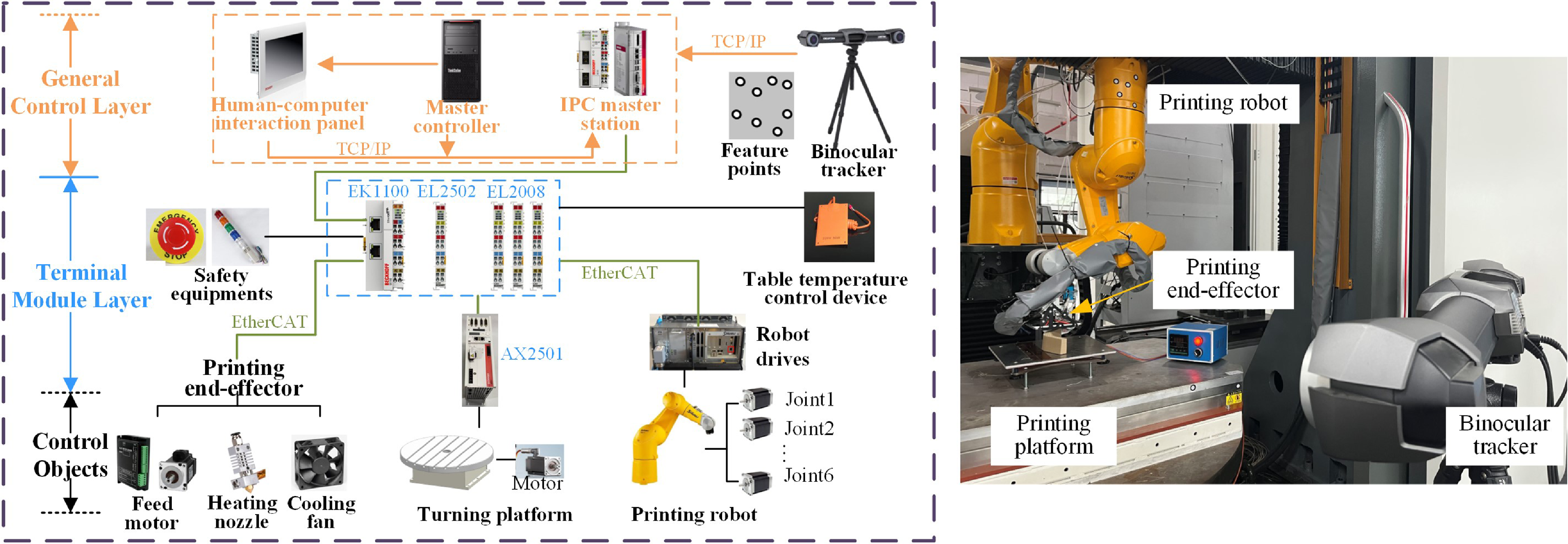
The robotic additive manufacturing platform was developed using Beckhoff industrial control software (TwinCAT), which provides an open and compatible robot control environment. By integrating a printing end-effector and a turntable, the robotic additive manufacturing system was constructed. Based on the EtherCAT bus protocol, the system is organized into three layers: the central control layer, the terminal module layer, and the controlled objects. The overall system framework and hardware compositions are depicted in Figure 9.
The central control layer comprises the master computer, the slave computer PLC (Programmable Logic Controller), and a human-computer interaction panel. The master computer is responsible for robot motion, printing planning, status collection, and hardware monitoring. The slave computer system supports the development of motion control algorithms and logic control programs. The interaction panel allows for manual debugging and automatic execution of the printing process.
The terminal module layer uses couplers and terminals to connect the central control layer with the control objects layer. The control objects include six motors of the robot, a turntable motor, and the key components of the end-effector. Motor-level control decomposes the robot into six independent motor units, which can be regulated in position, velocity, or torque mode. Additional controlled objects include safety devices and a substrate heating system for the printing platform. A binocular vision system provides real-time pose measurements, which are transmitted to the master controller via TCP/IP.
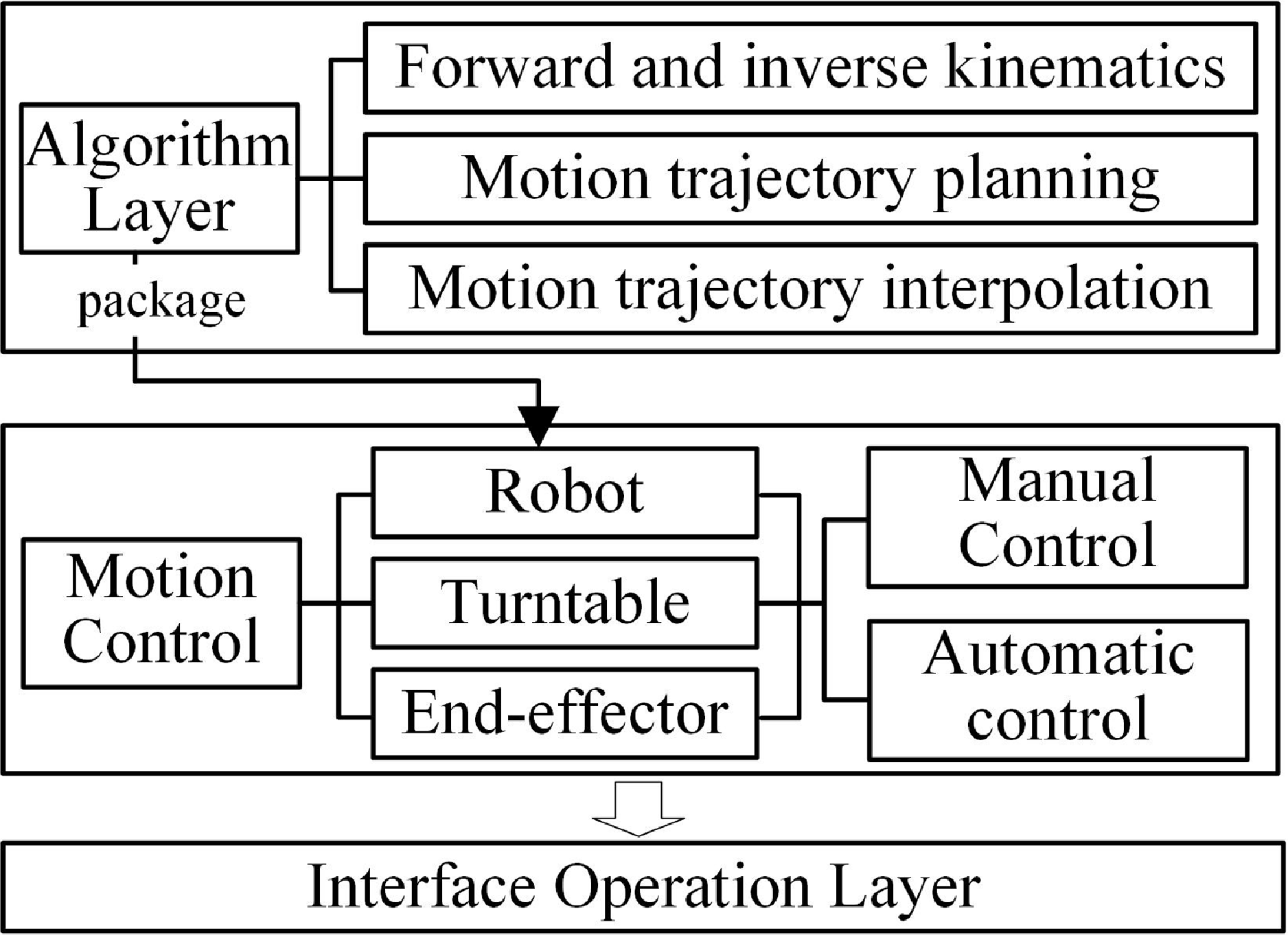
The control architecture comprises the robot algorithm layer, robot motion control layer, and interface operation layer, as shown in Figure 10. The control platform features both a manual debugging mode and an automatic execution mode. The interface operation layer facilitates the switching of control modes, enabling the jogging of the robot and printing turntable and the feeding of the wire feeding motor of the printing end-effector. The algorithm layer includes forward and inverse kinematics of the robot, the trajectory planning, and the interpolation of the end-effector, developed in Matlab/Simulink and deployed to TwinCAT software.
Calibration results of the TCP.

The hardware configuration for the robotic additive manufacturing system.
Control architecture of the additive manufacturing system.
3.2. Verification of visual servoing control
The results of the TCP in the wrist frame are shown in Table I. Nozzle 1 is located on the front, and Nozzle 2 is located on the rear side.
The theoretical and actual link lengths of TX90 robot.

The performance of the proposed visual servoing controller was evaluated using a BVI (C-track 780), visual reflectors, a Staubli TX90 robot, and the developed control system. The BVI provides continuous 3D measurements of reference reflectors with a sampling period of 20 ms. Its volumetric accuracy is 0.065 mm, and repeatability is 0.0025 mm, calibrated using a reference rod and Vxelements software. The Staubli TX90 robot has a maximum working radius of 1450 mm and a payload capacity of 14 kg. Its link parameters are shown in Table II, based on the method proposed in Ref. [Reference Tian, Mei, Li, Zeng, Hong and Zhou30], while joint limits and axis speed constraints are specified in the manufacturer’s manual. Trajectory planning and control algorithms were implemented in Twincat3 on the industrial computer (C6650-0060).
To validate the trajectory accuracy, three representative motion paths were tested: arc trajectory, linear trajectory, and continuous trajectory.
The multiple gains are given by
 $\mathrm{T} = \mathop {\textrm {diag}}\nolimits \left \{ {10} \right \}$
,
 ${\bar{\boldsymbol{K}}} = \mathop {\textrm {diag}}\nolimits \left \{ {0.5} \right \}$
, and
 $k_s=0.5$
. In light of the balance between prediction accuracy and solution speed, the number of nodes in the hidden layer is designed to be 7, and the value of the Gaussian function parameter is adjusted by
 $ {{\boldsymbol{C}}_i} = {\begin{bmatrix} {0.25}&{0.50}&{0.75}&{1.00}&{1.25}&{1.50}&{1.75}\end{bmatrix}}$
,
 ${b_i}=10$
. The weight update adaptive rate parameter is taken as
 ${{\boldsymbol{\Gamma }}_{MK}}={{\boldsymbol{\Gamma }}_{GK}} = \mathop {\textrm {diag}}\nolimits \left \{ {50} \right \}$
,
 ${{\boldsymbol{\Gamma }}_{CK}}=\mathop {\textrm {diag}}\nolimits \left \{ {2} \right \}$
.
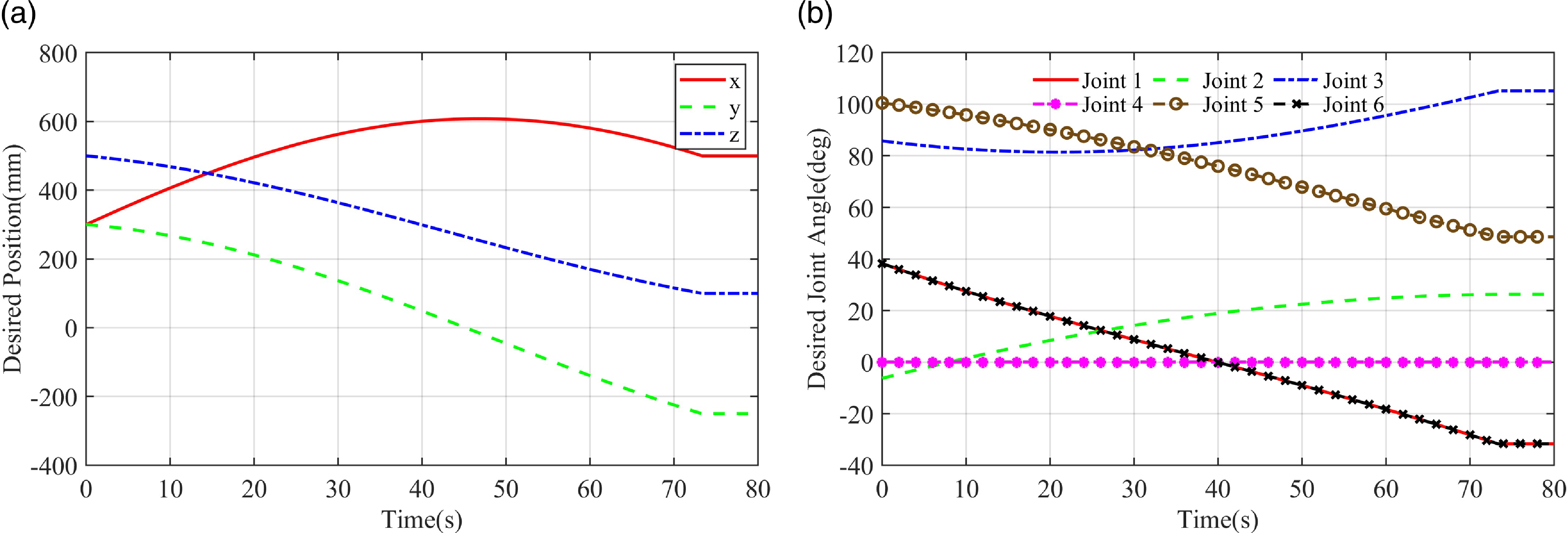
The arc trajectory was defined with a starting point (300, 300, 500), a midpoint (600, 50, 300), and an ending point (500, −250, 100). The maximum planned tangential speed is 10
 $\mathrm{mm/s}$
, with a tangential acceleration of 10
 $\mathrm{mm/{s^2}}$
. The time evolution of Cartesian coordinates is shown in Figure 11(a), and the time evolution of the joint space is shown in Figure 11(b).
Schematic diagram of the circular trajectory: (a) Interpolated curves in Cartesian space; (b) Interpolated curves in joint space.
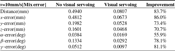
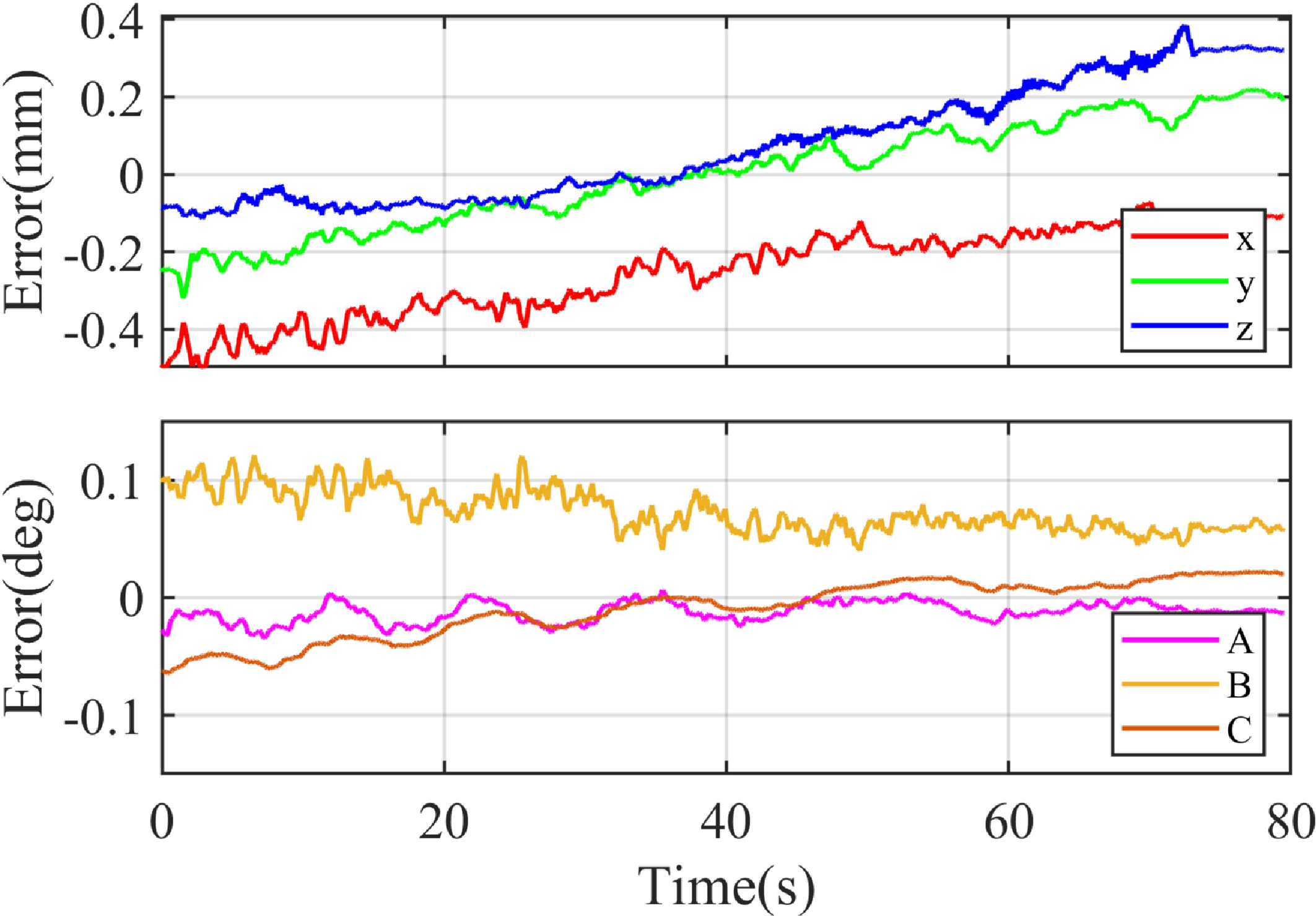
The pose tracking errors of the robot moving in an arc trajectory are displayed in Figs. 12 and 13. With visual servoing compensation, the position steady-state error is reduced to within
 $\pm$
0.1 mm, and the orientation error within
 $\pm$
0.05
 $^{\circ }$
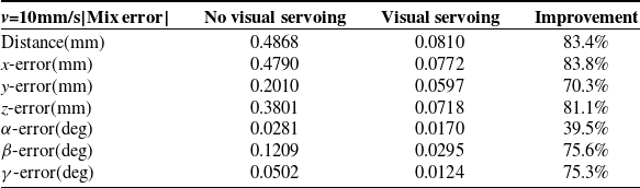
. Initial pose deviations converge to zero within 6 s. Without compensation, errors are larger and more irregular. A quantitative comparison of compensated and uncompensated circular motion is summarized in Table III.
Comparison of motion error in the stable state for circular trajectory.
Circular tracking error with visual servoing.

Circular tracking error without visual servoing.
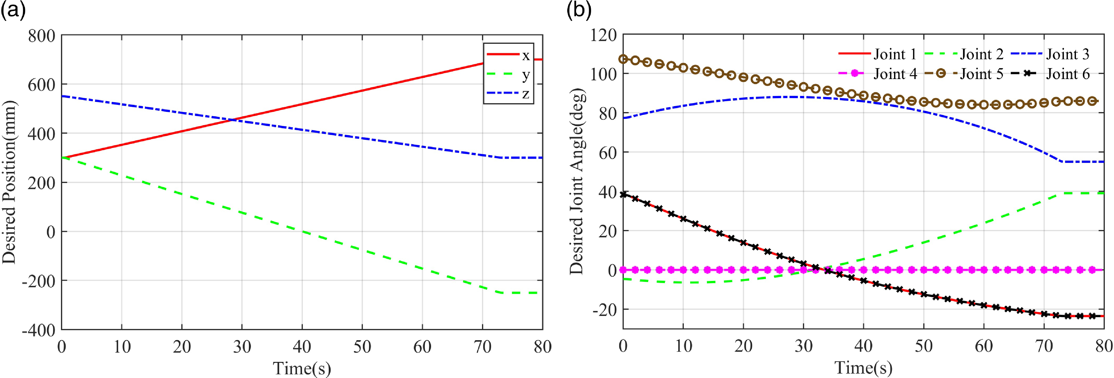
A linear trajectory was planned in the robot base frame, from (300, 300, 550) to (700, −250, 300), with a maximum velocity of 10 mm/s and an acceleration of 10
 $\mathrm{mm/s^2}$
. Cartesian and joint evolutions are shown in Figs. 14(a) and 14(b), respectively.
Schematic diagram of the linear trajectory: (a) Interpolated curves in Cartesian space; (b) Interpolated curves in joint space.
Linear tracking error with visual servoing.

Linear tracking error without visual servoing.
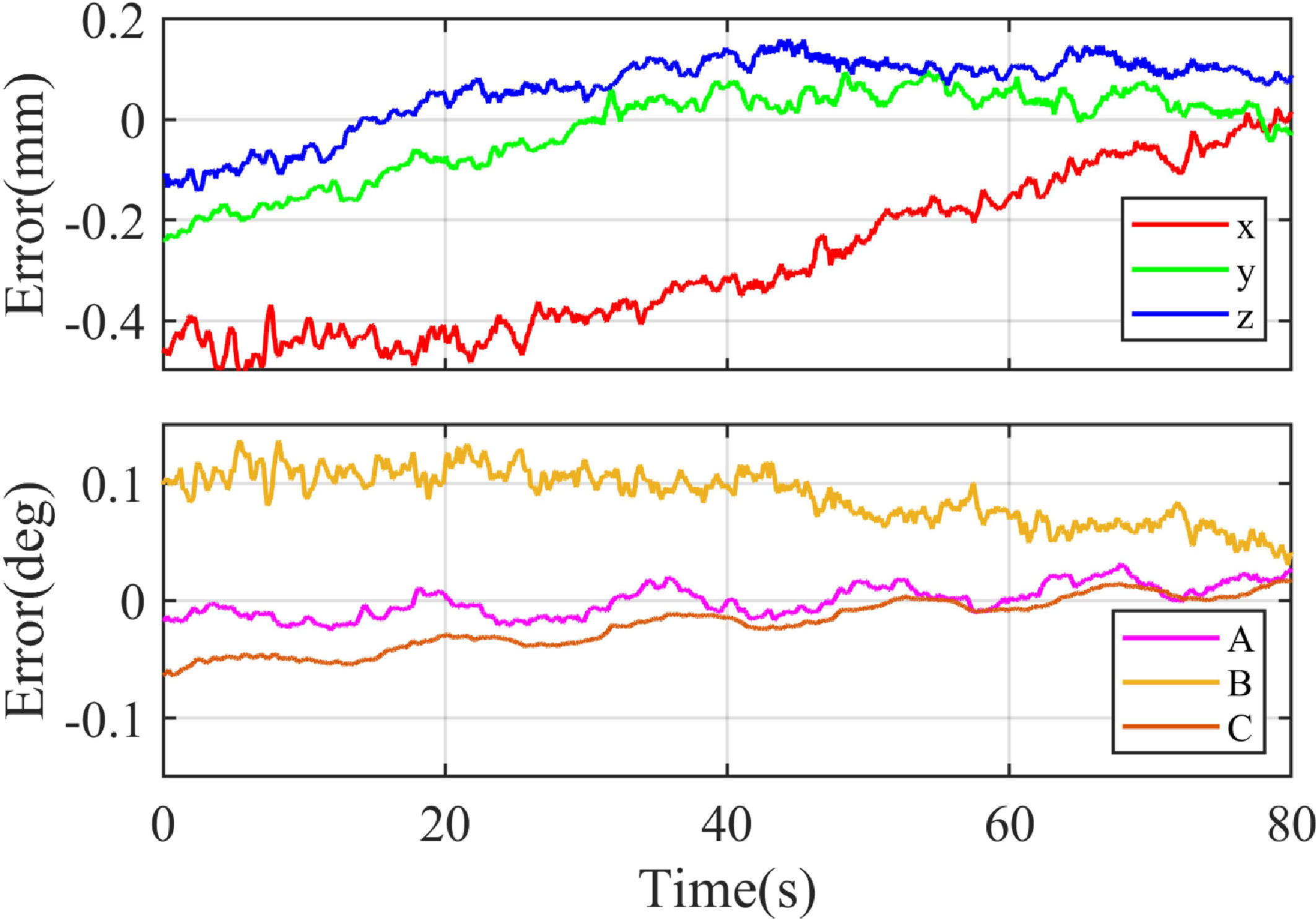
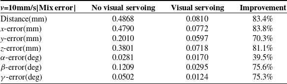
The tracking errors are displayed in Figs. 15 and 16, showing position errors below
 $\pm$
0.1 mm and rotation errors below
 $\pm$
0.05
 $^{\circ }$
. Compared with the uncompensated case, accuracy is markedly improved. Table IV summarizes the maximum steady-state errors for both conditions.
Comparison of motion error in the stable state for linear trajectory.
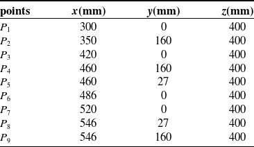
The coordinate value of trajectory sharp corner points.
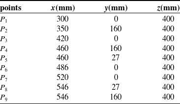
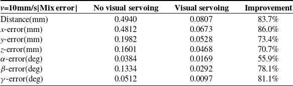
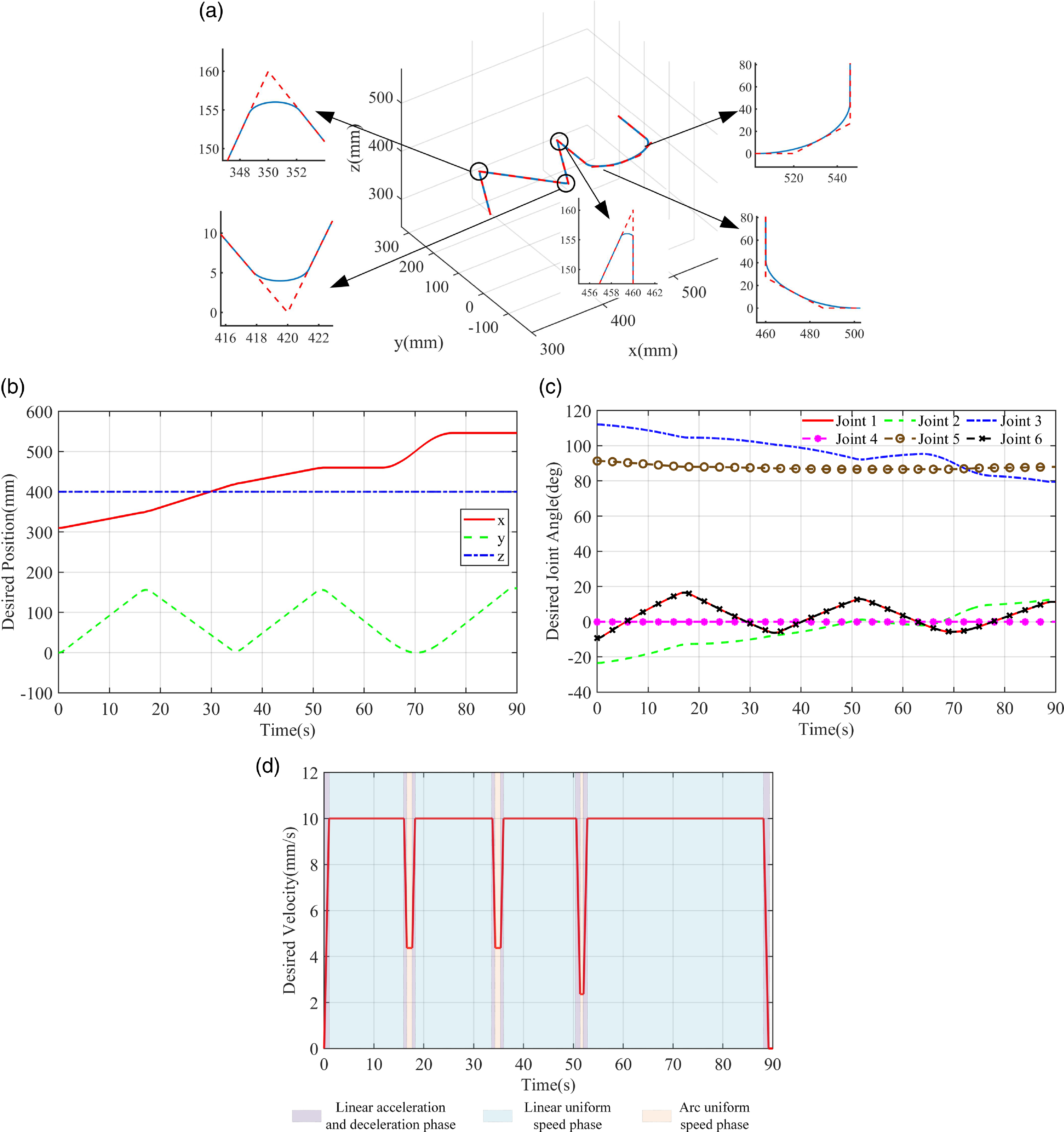
To evaluate corner tracking, a continuous trajectory with sharp turns was tested. The trajectory was smoothed using circular arc transitions, with a corner tolerance of 0.05 mm. Eight straight-line segments were combined to form the letter “NU,” with corner coordinates listed in Table V. The planned trajectories with and without arc transitions are illustrated in Figure 17(a). Cartesian and joint evolutions are shown in Figs. 17(b) and 17(c), and the Cartesian velocity profile in Figure 17(d). The velocity profile confirms continuity, as the end-effector did not decelerate to zero at the corners.
Schematic diagram of the continuous trajectory: (a) The trajectory in Cartesian space with and without arc transition; (b) Interpolated curves in Cartesian space; (c) Interpolated curves in joint space; (d) The speed in Cartesian space
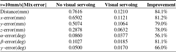
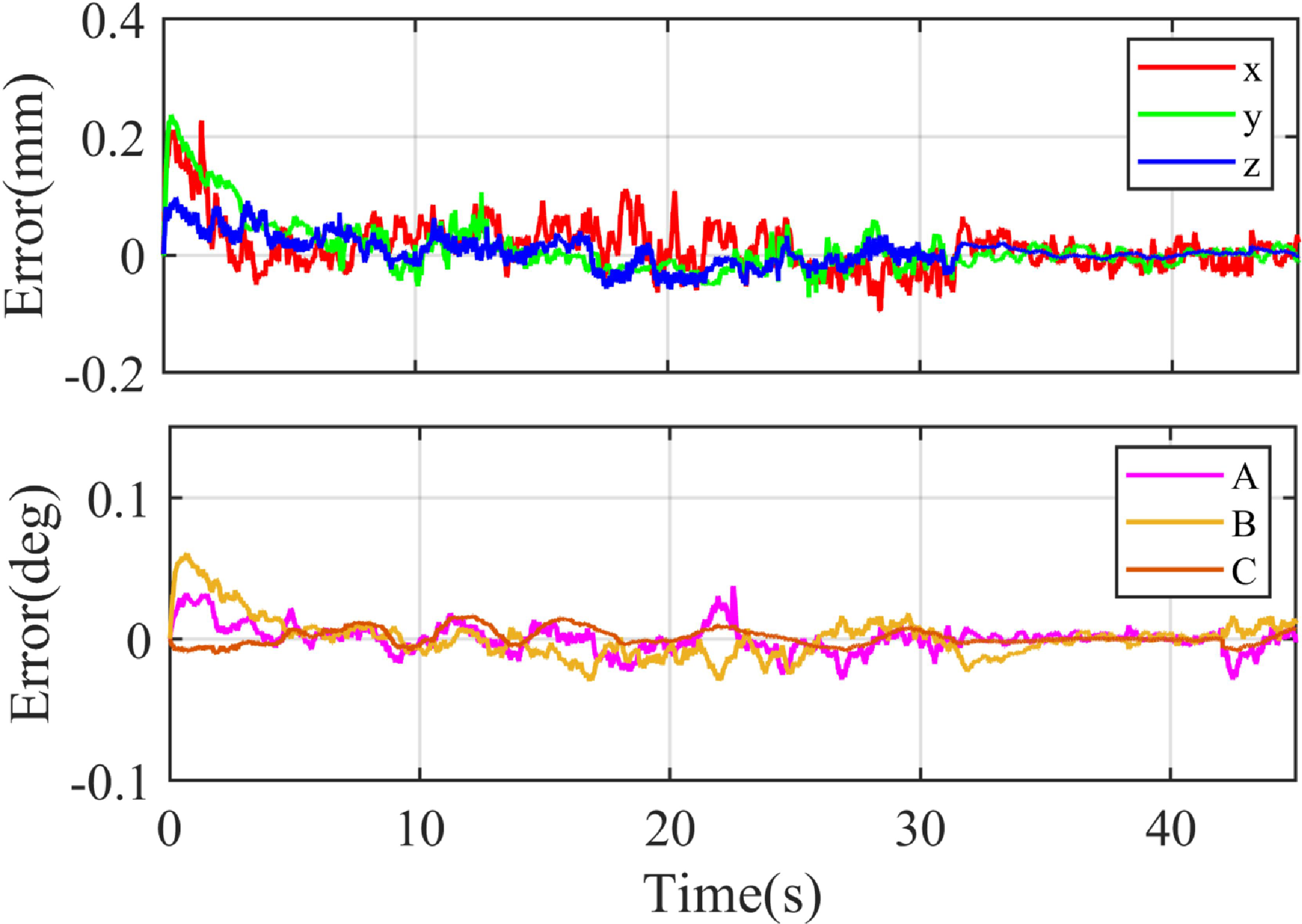
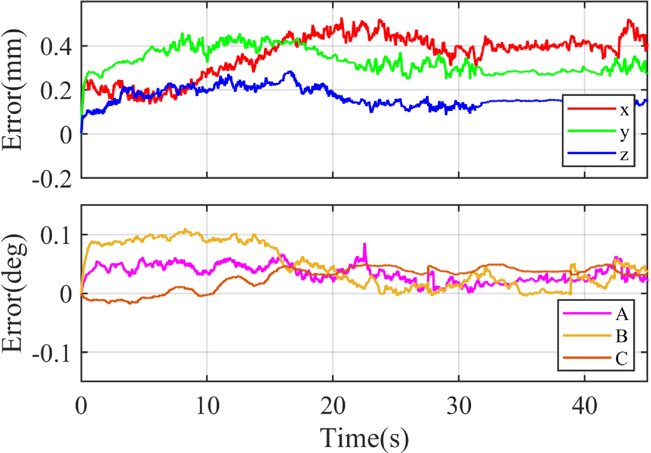
The corresponding tracking errors are presented in Figs. 18 and 19. With visual servoing, position errors remain below
 $\pm$
0.15 mm and rotation errors below
 $\pm$
0.05
 $^{\circ }$
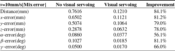
. Table VI compares the errors between compensated and uncompensated trajectories.
After the visual servoing compensation, the trajectory accuracy of the robot was improved to 0.121 mm without load for a continuous trajectory with corners. In the FDM additive manufacturing process, the load on the robot is negligible. Therefore, the improvement of the robot accuracy achieved by the method can be directly applied to the field of robot additive manufacturing, and the effectiveness was verified by the printing experiment presented in the following section.
3.3. Experiment for robotic additive manufacturing
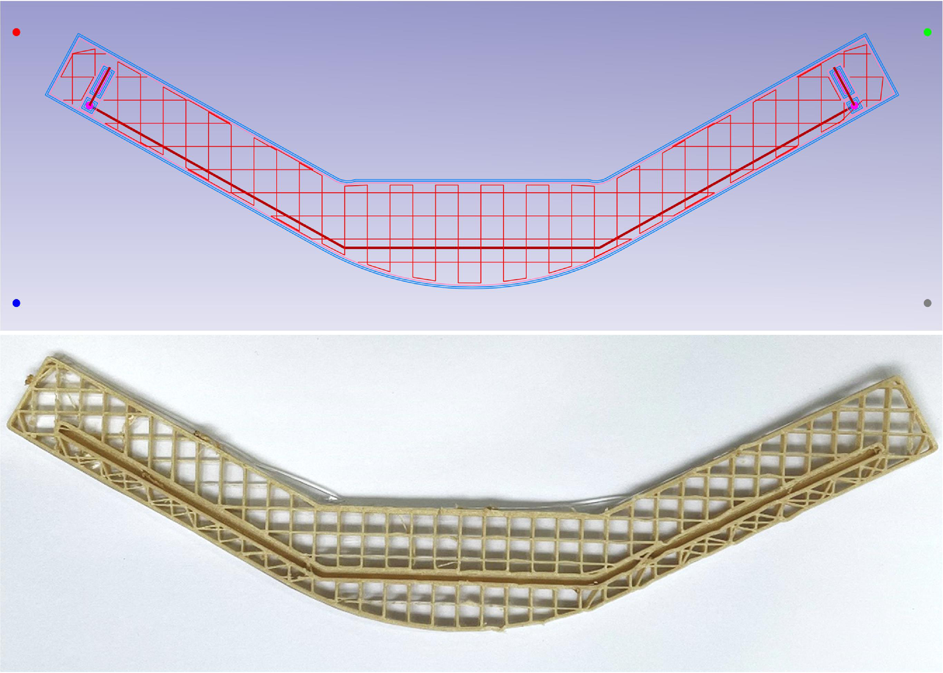
To further validate the method, a component was designed featuring both linear and curved characteristics, where the curved features can be approximated by a series of short straight lines. The printing path of the part is shown in Figure 20. The material used was PEEK, with a melting temperature of 320–390
 $^\circ C$
. Printing parameters were as follows: layer height 0.3 mm, wire feeding speed 7.5 mm/s, robot motion speed 10 mm/s, nozzle temperature 340
 $^\circ C$
, and platform temperature 150
 $^\circ C$
.
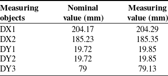
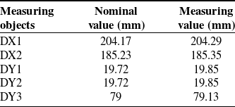
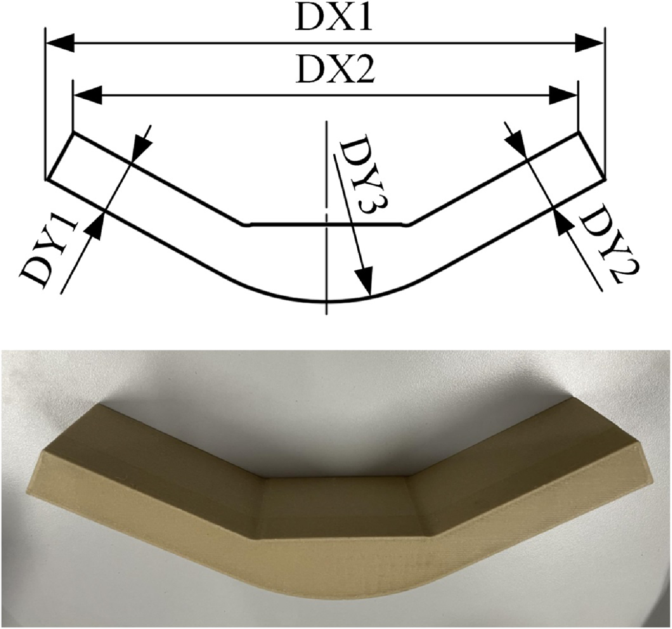
Microscopic inspection of printed parts is shown in Figure 21. Without compensation (Figure 21(a)), corner overflow and reduced trajectory straightness are evident. With the proposed method (Figure 21(b)), trajectory deviation and overflow are significantly reduced. Dimensional accuracy was evaluated using a coordinate measuring machine, with geometric dimensions annotated in Figure 22 and measurement results summarized in Table VII. The geometric error of the printed part was within
 $\pm$
0.15 mm.
These experiments demonstrate that visual servoing control, combined with arc transition smoothing, improves printing quality and enhances geometric accuracy. Thereby promoting the application of industrial robots in precision additive manufacturing of components.
4. Conclusion
In this article, a robotic additive manufacturing system is developed, integrating an industrial robot, a printing end-effector, and a turntable platform to enable effective collaborative control of multiple subsystems. A generalized non-parametric trajectory planning method is proposed to enhance the continuity and smoothness of robot motion, thereby enhancing the shape precision of printed components and reducing corner overflow. To address challenges related to limited NC code capacity and data transmission delays, a parallel planning architecture based on a register and planner mechanism is introduced. On the control side, the control strategy is employed, combining RBF neural network-based dynamic feedforward control with visual servoing feedback enhanced by a velocity observer. This framework improves both responsiveness and trajectory tracking accuracy under complex additive manufacturing paths. The stability of the control system is rigorously analyzed and proven using the Lyapunov method. The experimental results demonstrate that the trajectory planning technique significantly reduces geometric and shape-related errors, while the visual servoing-based tracking control achieves a position accuracy of
 $\pm$
0.15 mm and an orientation accuracy of
 $\pm$
0.05
 $^{\circ }$
, leading to notable improvements in manufacturing precision.
Future work will focus on improving the robustness of visual measurement under challenging environmental conditions, such as varying lighting, ambient disturbances, and partial object occlusion, to enhance the universality of the proposed method. In addition, advanced filtering strategies will be developed to improve the precision of visual servoing. Finally, tighter integration of equipment accuracy with the additive manufacturing process will be explored. These advancements are expected to facilitate broader industrial adoption of robotic systems.
Comparison of motion error in the stable state for continuous trajectory.
Continuous trajectory tracking error with visual servoing.
Continuous trajectory tracking error without visual servoing.
Measurement results of printed forming precision.
Robotic printing PEEK material.
Microscopic observation of the parts corner (a) without the method proposed in this paper; (b) with the method proposed in this paper.

Measurement results of printed forming precision.
Author contributions
Delan Wei: formal analysis, investigation, methodology, software, validation, data curation, and writing—original draft. Pengcheng Li: conceptualization, supervision, writing review & editing, and validation. Jun Xiong: supervision, writing review & editing. Yansheng Cao: investigation, resources. Xuewen Wei: software, data curation. Wei Tian: writing review & editing, validation, and resources. Wenhe Liao: conceptualization, supervision, validation, project management.
Financial support
This research was supported by the National Natural Science Foundation of China (No. 52205530), the Natural Science Foundation of Jiangsu Province (No. BK20210299), the Defense Industrial Technology Development Program of China under Grant (No. JCKY2021204B045), and the Key R&D plan of Jiangsu Province (No. BE2021090).
Competing interests
The authors declare no conflicts of interest exist.
Ethical approval
Not applicable.
Appendix A
In the RBFNNs,
 $\boldsymbol{x} = {[{x_i}]^T}$
and
 $\boldsymbol{h} = {[{h_j}]^T}$
are the inputs and outputs of the input layer and hidden layer of the networks, respectively. The output of the hidden layer is expressed as
 \begin{equation} {h_j} = \exp \left( { - \frac{{{{\left\| {{\mathrm{x}} - {c_j}} \right\|}^2}}}{{2b_j^2}}} \right)\end{equation}
where
 $\boldsymbol{c}$
represents the coordinate vector of the center point of the Gaussian basis function of the neuron, and
 $\boldsymbol{b}$
is the width of the Gaussian basis function of the neurons in the hidden layer.
The output of the RBFNNs is
 \begin{equation} y = {\boldsymbol{w}^T}\boldsymbol{h} = {w_1}{h_1} + {w_2}{h_2} + \cdots + {w_m}{h_m}\end{equation}
where
 $\boldsymbol{w}$
is the network weight,
 $\boldsymbol{w} = {[{w_1}, \cdots {w_m}]^T} $
.
Define
 \begin{equation}\begin{array}{l}{\boldsymbol{M}_x}(\boldsymbol{q}) = {\boldsymbol{F}_{MNN}}(\boldsymbol{q}) + {\boldsymbol{E}_M}\\[5pt]{\boldsymbol{C}_x}(\boldsymbol{q},\dot{\boldsymbol{q}}) = {\boldsymbol{F}_{CNN}}(\boldsymbol{q},\dot{\boldsymbol{q}}) + {\boldsymbol{E}_C}\\[5pt]{\boldsymbol{G}_x}(\boldsymbol{q}) = {\boldsymbol{F}_{GNN}}(\boldsymbol{q}) + {\boldsymbol{E}_G}\end{array}\end{equation}
where
 $\boldsymbol{E}_M$
,
 $\boldsymbol{E}_C$
,
 $\boldsymbol{E}_G$
are the modeling error of
 $\boldsymbol{M}_x (\boldsymbol{q})$
,
 $\boldsymbol{C}_x (\boldsymbol{q},\dot{\boldsymbol{q}})$
,
 $\boldsymbol{G}_x (\boldsymbol{q})$
by the RBFNNs, respectively.
The estimation for
 $\boldsymbol{F}_{MNN} (\boldsymbol{q})$
,
 $\boldsymbol{F}_{CNN} (\boldsymbol{q},\dot{\boldsymbol{q}})$
and
 $\boldsymbol{F}_{GNN} (\boldsymbol{q})$
are
 \begin{equation}\begin{array}{l}{\hat{\boldsymbol{F}}_{MNN}} = \hat{\boldsymbol{w}}_M^T \cdot {\boldsymbol{h}_M}(\boldsymbol{q})\\[5pt]{\hat{\boldsymbol{F}}_{CNN}} = \hat{\boldsymbol{w}}_C^T \cdot {\boldsymbol{h}_C}(\boldsymbol{z})\\[5pt]{\hat{\boldsymbol{F}}_{GNN}} = \hat{\boldsymbol{w}}_G^T \cdot {\boldsymbol{h}_G}(\boldsymbol{q})\end{array}\end{equation}
where
 ${\hat{\boldsymbol{w}}_M}$
,
 ${\hat{\boldsymbol{w}}_C}$
and
 ${\hat{\boldsymbol{w}}_G}$
are the estimated value of the neural networks weight, and
 ${\boldsymbol{h}_M}(\boldsymbol{q})$
,
 ${\boldsymbol{h}_C}(\boldsymbol{z})$
and
 ${\boldsymbol{h}_G}(\boldsymbol{q})$
are the kernel function matrix of the neural networks, where
 $\boldsymbol{z} = {\begin{bmatrix} \boldsymbol{q}&\dot{\boldsymbol{q}}\end{bmatrix}^T}$
.