1 Introduction
A bore is a propagating transition between two streams. Denoting by 1 the state ahead of the bore, and by and 2 the state behind it, the two streams are characterized by different water depths
 $h_{1}$
and
 $h_{2}$
, with
 $h_{1}<h_{2}$
. The intensity of two-dimensional (vertical plane) bores is mainly characterized by the Froude number
 $$\begin{eqnarray}Fr={\displaystyle \frac{|u_{1}-c_{b}|}{\sqrt{gh_{1}}}},\end{eqnarray}$$
where
 $u$
is the depth averaged velocity and
 $c_{b}$
the bore celerity. For large
 $Fr$
the jump observed corresponds to a turbulent breaking wave. For
 $Fr$
smaller than approximately 1.3, the bore transition is smooth and followed by wave trains. The bore is hence made of a mean jump between two water depths on which secondary waves are superimposed. This type of bore is usually named an undular bore. Favre (Reference Favre1935) was the first to describe this phenomenon from laboratory experiments. That is why undular bores are sometimes referred to as Favre waves. This phenomenon is a weakly dispersive non-hydrostatic process which can be modelled by Boussinesq-type equations (e.g. Peregrine Reference Peregrine1966). In the mathematical community this dispersive process is also named dispersive shock. The dynamics of two-dimensional undular bores has been extensively studied from laboratory experiments (e.g. Favre Reference Favre1935; Treske Reference Treske1994; Gourlay Reference Gourlay2001; Soares Frazao & Zech Reference Soares Frazao and Zech2002; Chanson Reference Chanson2009), theoretical (e.g. Lemoine Reference Lemoine1948; Benjamin & Lighthill Reference Benjamin and Lighthill1954; Johnson Reference Johnson1972; El, Grimshaw & Smyth Reference El, Grimshaw and Smyth2006) and numerical approaches (e.g. Peregrine Reference Peregrine1966; Wei et al.
Reference Wei, Kirby, Grilli and Subramanya1995; Soares Frazao & Zech Reference Soares Frazao and Zech2002; Tissier Reference Tissier2011; Kazolea & Ricchiuto Reference Kazolea and Ricchiuto2018; Shi et al.
Reference Shi, Malej, Smith and Kirby2018).
Schematic representation of the cross-section of natural alluvial channels;
 $W$
is the bottom channel width,
 $\unicode[STIX]{x1D6FD}$
the bed-slope angle from horizontal,
 $h_{1}$
and
 $h_{2}$
are the water depths ahead and behind the bore respectively.

However, natural estuary and river channels are non-rectangular and present most of the time a variable cross-section with a nearly trapezoidal shape and gently sloping banks (see figure 1). The bore dynamics is then mainly controlled by three dimensionless parameters among which are the Froude number (1.1), and the geometrical parameters
 $W/h_{1}$
and
 $\tan \unicode[STIX]{x1D6FD}$
, where
 $W$
and
 $\unicode[STIX]{x1D6FD}$
are the characteristic bottom channel width and bed-slope angle from horizontal respectively. Only a few studies have been devoted to undular bore dynamics in channels with variable cross-section. The propagation of undular bores over a trapezoidal cross-section channel, with fixed parameters
 $\unicode[STIX]{x1D6FD}=1/3$
and
 $W/h_{1}=7.75$
, was studied by Treske (Reference Treske1994). He showed that the secondary wave field is two-dimensional with strong variations in crest height across the channel section, and then strongly differs from that in rectangular channels. Treske (Reference Treske1994) identified a transition around
 $Fr_{t}=1.15$
. For
 $F<Fr_{t}$
, the secondary wave wavelength in the whole channel is at least two to three times larger than in a rectangular channel for the same Froude numbers. For
 $F>Fr_{t}$
however the secondary wave field along the channel axis becomes very similar to Favre waves (rectangular channels), while long wavelengths are still observed along the banks, leading to a complex multi-dimensional wave structure. In field observations a similar transition was described for the first time in long-term high-frequency experiments carried out in the two main French tidal bore estuaries: the Seine and Gironde/Garonne estuaries (see Bonneton et al.
Reference Bonneton, Parisot, Bonneton, Sottolichio, Castelle, Marieu, Pochon and de Loock2011, Reference Bonneton, Bonneton, Parisot, Sottolichio and Detandt2012, Reference Bonneton, Bonneton, Parisot and Castelle2015). The authors identified two undular bore regimes around a transition Froude number
 $Fr_{t}$
of approximately 1.1: the high Froude number regime (HFN regime) for
 $F>Fr_{t}$
and the low Froude number regime (LFN regime) for
 $F<Fr_{t}$
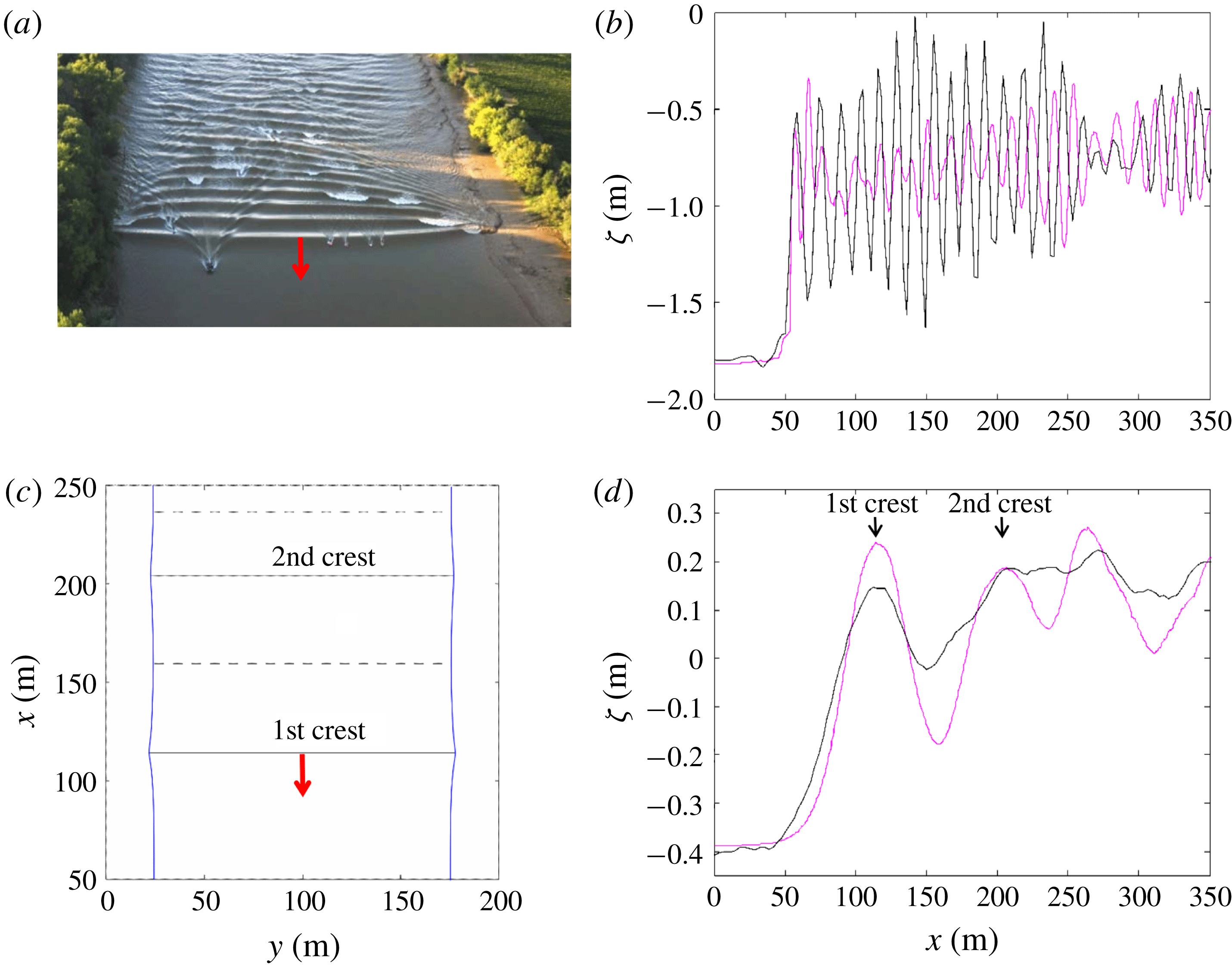
. In the HFN regime, the secondary wave field is strongly multi-dimensional and characterized by a ‘fish-tail’ pattern (see figure 2
a). The wave amplitude is maximum in the mid-channel and decreases toward the banks (figure 2
b). It was shown that the amplitude and wavelength along the river axis are similar to those of Favre waves in rectangular channels for the same Froude number. This observation indicates that this HFN regime is most probably controlled by dispersive non-hydrostatic processes as for the Favre waves. The secondary wave field in the LFN regime shows a significantly different behaviour. The phase structure is quasi-one-dimensional (figure 2
c), and the wave amplitude is at its maximum on the banks and minimum in the mid-channel (figure 2
d). The transition between HFN and LFN regimes is marked by an abrupt decrease of the secondary wave steepness (Bonneton et al.
Reference Bonneton, Bonneton, Parisot and Castelle2015), and by a considerable increase in wavelength. The low wave steepness of the LFN makes visual observations of undular tidal bores very difficult. This is why tidal bore occurrence in worldwide estuaries is certainly underestimated (Bonneton et al.
Reference Bonneton, de Loock, Parisot, Bonneton, Sottolichio, Detandt, Castelle, Marieu and Pochon2011a
, Reference Bonneton, Bonneton, Parisot and Castelle2015).
Illustration of the two undular tidal bore regimes (Garonne River, Bonneton et al.
Reference Bonneton, Bonneton, Parisot and Castelle2015). (a,b) High Froude number regime (
 $Fr=1.27$
); (c,d) low Froude number regime (
 $Fr=1.08$
). (a) Two-dimensional (2-D) phase structure; (c) quasi-1-D phase structure. Black line, elevation in the mid-channel; magenta line, elevation close to the bank.

In this paper, a detailed analysis of undular bore dynamics in channels of variable cross-section is presented. The two undular bore regimes (LFN and HFN) are simulated with a Serre–Green–Naghdi model, and the results are compared with Treske’s experiments. We show that contrary to Favre waves and HFN bores, which are controlled by dispersive non-hydrostatic mechanisms, the LFN bores correspond to an hydrostatic phenomenon. The dispersive-like properties of the LFN bores are related to wave refraction on the banks in a way similar to those of edge waves in the near shore. A fully hydrostatic asymptotic model for these dispersive-like bores (i.e. LFN bores) is derived and compared to the observations, confirming our claim.
2 Dispersive wave modelling
2.1 Mathematical and numerical model
The generation of undular bores is in general related to non-hydrostatic propagation and thus it requires the use of dispersive equations to be correctly modelled. In this work we use a phase-enhanced fully nonlinear and weakly dispersive Serre–Green–Naghdi model which can be recast as (Filippini, Kazolea & Ricchiuto Reference Filippini, Kazolea and Ricchiuto2016, Reference Filippini, Kazolea and Ricchiuto2017a ):
 $$\begin{eqnarray}\left.\begin{array}{@{}c@{}}{\displaystyle \frac{\unicode[STIX]{x2202}\unicode[STIX]{x1D701}}{\unicode[STIX]{x2202}t}}+\unicode[STIX]{x1D735}\boldsymbol{\cdot }(h\boldsymbol{u})=0,\\ {\displaystyle \frac{\unicode[STIX]{x2202}(h\boldsymbol{u})}{\unicode[STIX]{x2202}t}}+\unicode[STIX]{x1D735}\boldsymbol{\cdot }(h\boldsymbol{u}\otimes \boldsymbol{u})+gh\unicode[STIX]{x1D735}\unicode[STIX]{x1D701}=\unicode[STIX]{x1D753},\end{array}\right\}\end{eqnarray}$$
where
 $\unicode[STIX]{x1D701}$
denotes the free surface elevation,
 $h$
the water depth and
 $\boldsymbol{u}$
the depth averaged horizontal velocity vector of
 $\boldsymbol{u}=(u,v)$
. The term
 $\unicode[STIX]{x1D753}$
represents the non-hydrostatic effects, and can be shown to be the solution of an auxiliary elliptic partial differential equation which can be written as
 $$\begin{eqnarray}\unicode[STIX]{x1D753}+\unicode[STIX]{x1D6FC}T(\unicode[STIX]{x1D753})=T(gh\unicode[STIX]{x1D735}\unicode[STIX]{x1D701})-Q(\boldsymbol{u}),\end{eqnarray}$$
where
 $\unicode[STIX]{x1D6FC}$
is a tuning parameter used to enhance the linear frequency dispersion and shoaling characteristics of the model (Chazel, Lannes & Marche Reference Chazel, Lannes and Marche2011). The value
 $\unicode[STIX]{x1D6FC}=1.159$
provides relative phase errors below 1 % for reduced wavenumbers up to
 ${\approx}\unicode[STIX]{x03C0}$
. The definitions of the differential operators
 $T(\unicode[STIX]{x1D74E})$
and
 $Q(\unicode[STIX]{x1D74E})$
are reported for completeness in appendix A, following Lannes & Marche (Reference Lannes and Marche2015), Filippini et al. (Reference Filippini, Kazolea and Ricchiuto2016, Reference Filippini, Kazolea and Ricchiuto2017a
). For
 $\unicode[STIX]{x1D753}=0$
the system reduces to the hydrostatic, hyperbolic Saint–Venant/shallow water model.
The coupled system (2.1)–(2.2) is solved numerically on unstructured grids using the two step hybrid strategy proposed in Filippini et al. (Reference Filippini, Kazolea and Ricchiuto2016, Reference Filippini, Kazolea and Ricchiuto2017a
). In this approach the first step consists of recovering the non-hydrostatic correction by solving the elliptic problem (2.2) using a finite element method based on the symmetric variational form exploiting the self-adjoint character of the operator
 $T$
(see Alvarez-Samaniego & Lannes (Reference Alvarez-Samaniego and Lannes2008), Filippini et al. (Reference Filippini, Kazolea and Ricchiuto2016) for details). Once
 $\unicode[STIX]{x1D753}$
is known, the evolutionary partial differential equations (2.1) are solved by means of a third-order finite volume method, combined with a third-order strong stability preserving Runge–Kutta or with a fourth-order Adams–Bashforth/Adams–Moulton predictor corrector method to march in time. The resulting algorithm has been shown to have discrete linear dispersion properties comparable to those of a fourth-order finite difference discretization (Filippini et al.
Reference Filippini, Kazolea and Ricchiuto2016; Filippini, Kazolea & Ricchiuto Reference Filippini, Kazolea and Ricchiuto2017b
).
Finally, wave breaking is modelled by means of the shock capturing approach also used in Tonelli & Petti (Reference Tonelli and Petti2009), Shi et al. (Reference Shi, Kirby, Harris, Geiman and Grilli2012), Tissier et al. (Reference Tissier, Bonneton, Marche, Chazel and Lannes2012), Kazolea, Delis & Synolakis (Reference Kazolea, Delis and Synolakis2014), Filippini et al. (Reference Filippini, Kazolea and Ricchiuto2016): the non-hydrostatic correction
 $\unicode[STIX]{x1D753}$
is set to zero in regions flagged as breaking. This allows the formation of dissipative bores/shocks across which the total energy is dissipated, with a rate very close to the one encountered in the surf region (Bonneton Reference Bonneton2007). The flagging is performed by means of the physical criteria suggested in Kazolea et al. (Reference Kazolea, Delis and Synolakis2014), which make use of the norm of the gradient of the time derivative of the free surface
 $\unicode[STIX]{x1D701}$
, and of a limiting of the breaking region based on a minimum local Froude number of approximately 1.3 as proposed in Tissier et al. (Reference Tissier, Bonneton, Marche, Chazel and Lannes2012).
2.2 Undular bores simulations in straight-walled channels
As a preliminary step toward the main application of the paper, we consider the simulation of undular bores in channels with a rectangular section. Even though our numerical model has been thoroughly validated in the original references, this straight-walled case provides a simple benchmark involving undular bores. The resulting simulations will lead to clarification of some interesting aspects related to this type of benchmark, which have never been explicitly addressed.
We first reproduce the three undular bore configurations proposed in Wei et al. (Reference Wei, Kirby, Grilli and Subramanya1995), and then provide a more thorough study of the dependence of bore characteristics on the Froude number.
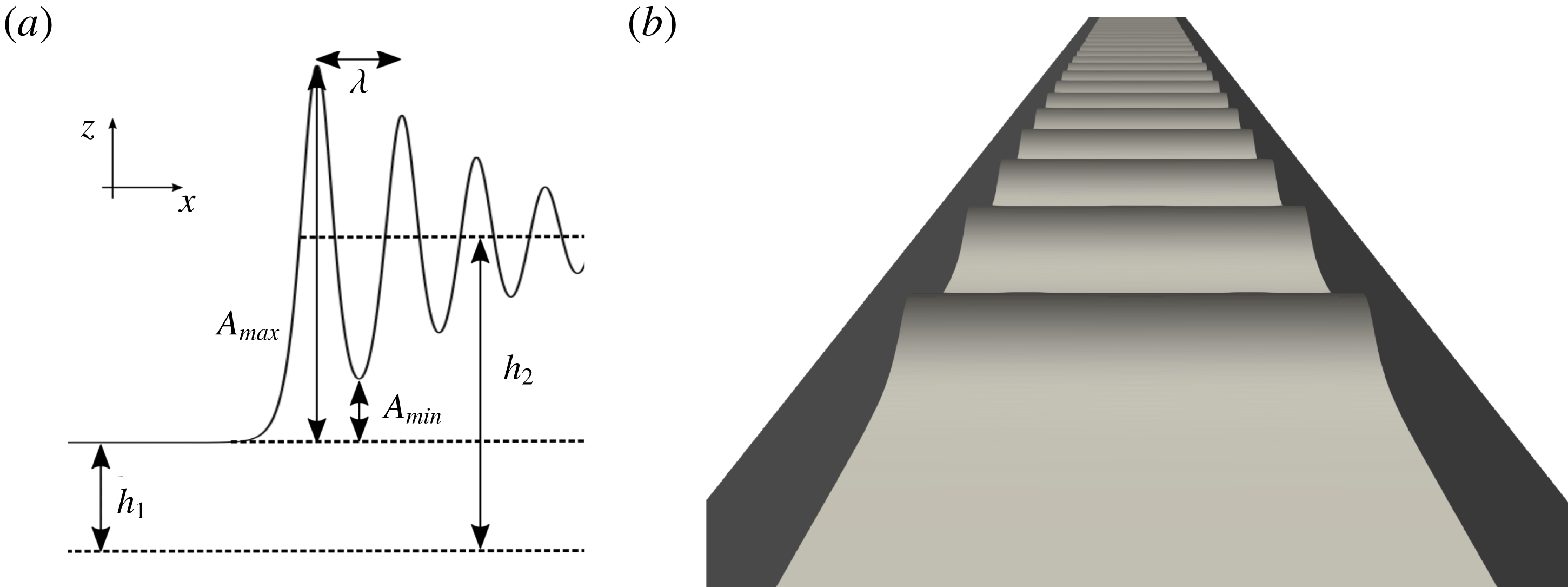
Bore in a channel of rectangular section. (a) Main physical parameters, (b) typical undular bore free surface.

A sketch of the problem with the notation for the most relevant physical parameters is reported in figure 3(a), while the typical undular bore free surface is displayed in figure 3(b). The initial condition used in the numerical simulations is defined by a mean hydrostatic bore satisfying the Rankine–Hugoniot relations associated with the Saint–Venant system. Denoting the states ahead and behind the bore with subscripts 1 and 2, these conditions read:
 $$\begin{eqnarray}\left.\begin{array}{@{}c@{}}u_{1}-c_{b}=-\left({\displaystyle \frac{gh_{2}}{2h_{1}}}(h_{1}+h_{2})\right)^{1/2},\\ u_{2}-c_{b}=-\left({\displaystyle \frac{gh_{1}}{2h_{2}}}(h_{1}+h_{2})\right)^{1/2}.\end{array}\right\}\end{eqnarray}$$
For all the computations of this section we have used a rectangular computational domain of dimensions
 $[100\times 2]~\text{m}^{2}$
, and a regularization of the initial discontinuity defined as
 $$\begin{eqnarray}\left.\begin{array}{@{}c@{}}h(x,y,t=0)={\displaystyle \frac{h_{2}-h_{1}}{2}}\tanh ((x-x_{0})/l_{t})+h_{2},\\ u(x,y,t=0)={\displaystyle \frac{u_{2}-u_{1}}{2}}\tanh ((x-x_{0})/l_{t})+u_{2}\\ v(x,y,t=0)=0,\end{array}\right\}\end{eqnarray}$$
where
 $x_{0}=95$
m and
 $l_{t}=0.5$
m. Periodic boundary conditions are used in the
 $y$
direction, and for all cases we have used
 $u_{1}=0~\text{m}~\text{s}^{-1}$
and
 $h_{1}=0.16$
m. Concerning the discretization, the reference grid sizes in the longitudinal and transversal axis are
 $\unicode[STIX]{x1D6FF}_{x}=0.04$
m and
 $\unicode[STIX]{x1D6FF}_{y}=0.5$
m. These sizes have been chosen to have at least twenty grid points per wavelength in all computations. We have numerically verified that for these values the flow characteristics, including the wavelengths measured, are converged.
We start by considering the three configurations discussed in § 5.2 of Wei et al. (Reference Wei, Kirby, Grilli and Subramanya1995), defined by the value of the nonlinearity ratio
 $\unicode[STIX]{x1D716}=(h_{2}-h_{1})/h_{1}$
. The values used are
 $\unicode[STIX]{x1D716}_{1}=0.1$
,
 $\unicode[STIX]{x1D716}_{2}=0.2$
, and
 $\unicode[STIX]{x1D716}_{3}=0.3$
. We can use relations (2.3) and the definition of Froude number (1.1) to show that the computations correspond to
 $Fr_{1}\approx 1.07$
,
 $Fr_{2}\approx 1.15$
and
 $Fr_{3}\approx 1.22$
.
As in the reference we visualize the ratio
 $\unicode[STIX]{x1D701}/h_{1}$
as a function of
 $x^{\prime }=x/h_{1}$
, at three different values of the non-dimensional time
 $t^{\prime }=t/\sqrt{h_{1}/g}$
:
 $t^{\prime }=50$
,
 $t^{\prime }=60$
and
 $t^{\prime }=70$
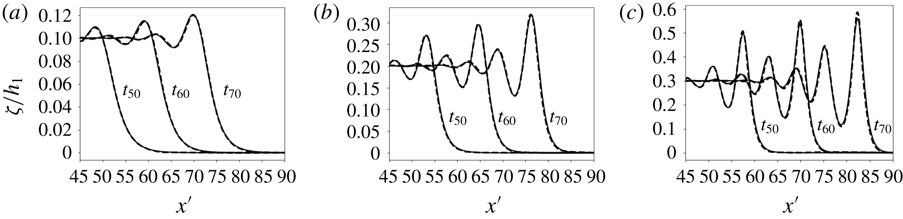
. We report in figure 4 a comparison of our numerical results with the fully nonlinear potential flow solutions reported in Wei et al. (Reference Wei, Kirby, Grilli and Subramanya1995), used here as a reference. We can see the increase in the amplitude of the secondary waves as nonlinearity increases. The fully nonlinear and weakly dispersive model used here does an excellent job in capturing the amplitudes of these waves. We also remark that the wavelengths provided by our model match very well those of the reference, despite its weakly dispersive character. The small underestimation of the amplitude for the most nonlinear case is consistent with the results obtained in Wei et al. (Reference Wei, Kirby, Grilli and Subramanya1995) with a different fully nonlinear Boussinesq model.
Undular bore propagation (from Wei et al.
Reference Wei, Kirby, Grilli and Subramanya1995). (a)
 $\unicode[STIX]{x1D716}_{1}=0.1$
, (b)
 $\unicode[STIX]{x1D716}_{2}=0.2$
, (c)
 $\unicode[STIX]{x1D716}_{3}=0.3$
. Continuous line: numerical results obtained here. Dashed line: reference fully nonlinear/fully dispersive potential solution (from Wei et al. (Reference Wei, Kirby, Grilli and Subramanya1995) reproduced with permission of the authors).

With the same set-up, we perform an investigation similar to the one done experimentally by Favre (Reference Favre1935) and Treske (Reference Treske1994) in rectangular flumes. Several simulations are performed for values of the Froude number from 1.01 to 1.30. The quantities compared to the experimental data are (cf. figure 3
a) the wave heights
 $A_{max}$
and
 $A_{min}$
, the amplitude
 $2A=A_{max}-A_{min}$
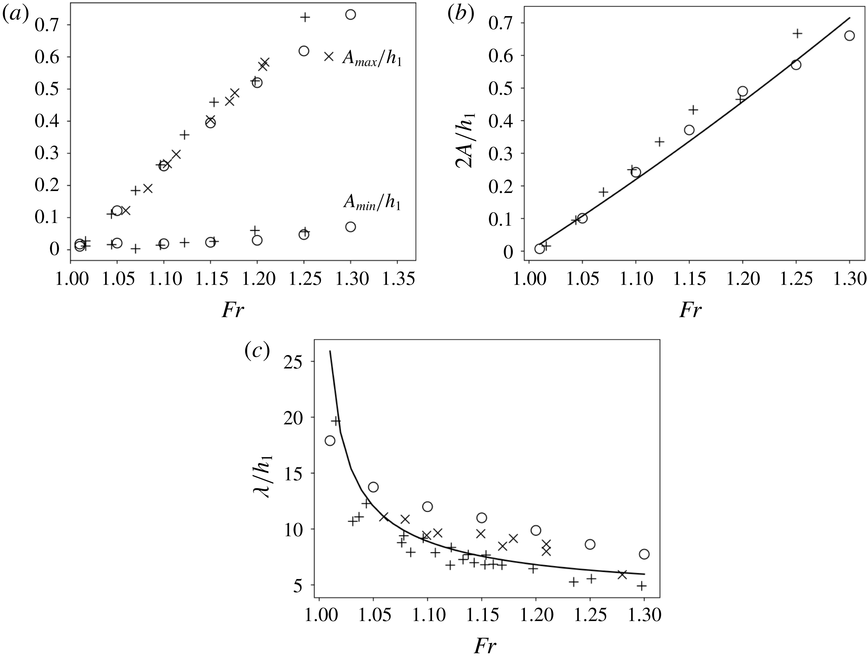
and the wavelength. The resulting comparisons between our simulations, the experimental data from Favre (Reference Favre1935) and Treske (Reference Treske1994), and the well-known theory by Lemoine (Reference Lemoine1948), are reported in figure 5.
Undular bore propagation. (a) Water heights, (b) amplitude, (c) wavelength.
 $+$
: data of Treske (Reference Treske1994),
 $\times$
: Favre (Reference Favre1935), ○: numerical simulations, ——: Lemoine (Reference Lemoine1948) theory.

The water level elevations
 $A_{max}$
and
 $A_{min}$
fit very well the data of Favre (Reference Favre1935) and Treske (Reference Treske1994). The same can be said for the amplitudes, reported in figure 5(b). The figure also shows that an excellent estimation of the amplitude can be obtained from the theory by Lemoine (Reference Lemoine1948). Concerning the wavelengths, in figure 5(c) we can see that our simulations provide a good prediction of the magnitudes, as well as of the wavelength reduction for increasing
 $Fr$
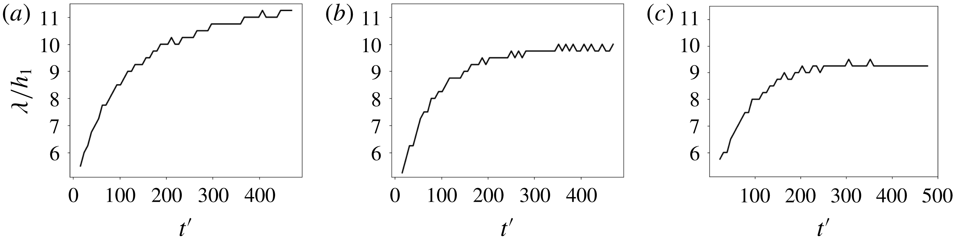
. The agreement is however less striking than for the water elevation, the numerical results providing a wavelength overestimation. This is somewhat surprising as the values of the reduced wavenumber of the secondary waves is of the order of 0.6–1.0, which is well within the validity of our model. Note however, the same discrepancy has been observed by other authors in simulations obtained with models similar to ours, as in the PhD thesis of Tissier (Reference Tissier2011), as well as in full Navier–Stokes simulations, as in Putra et al. (Reference Putra, Beaudoin, Rousseaux, Thomas and Huberson2019). This mismatch is most probably due to the fact that the wavelength after the initial bore formation increases with time. This dependency is clearly measurable in our simulations, as shown in figure 6 for Froude numbers similar to those of figure 4. This dependence is not explicitly accounted for in the experiments by Favre (Reference Favre1935) and Treske (Reference Treske1994). Despite this discrepancy, the comparisons of figures 4 and 5 are extremely satisfactory in terms of validation of our model. A more detailed investigation of the dynamics of undular bores of Green–Naghdi models is beyond the scope of this paper, and is left for future work.
Undular bore propagation: evolution of the measured wavelength with the propagation time. (a)
 $Fr=1.15$
, (b)
 $Fr=1.2$
, (c)
 $Fr=1.22$
.

3 Bore propagation in trapezoidal channels
The secondary wave field in rectangular channels simulated in the previous section is a dispersive non-hydrostatic phenomenon (a dispersive shock). As discussed in the introduction, the bore dynamics drastically change when topographic variations along the channel cross-section are present, as shown by Treske (Reference Treske1994) in laboratory experiments, and by Bonneton et al. (Reference Bonneton, Bonneton, Parisot and Castelle2015) in field observations. To show that we can model this dynamics with a weakly dispersive Serre–Green–Naghdi approach, in this section we reproduce numerically the experiments by Treske. As we will see, the simulations reproduce the transition between the high Froude number (HFN) and low Froude number (LFN) regimes discussed in the introduction. The comparison between simulations and experimental data provides some further insight into the differences between these two regimes, leading to the conclusion that the LFN secondary waves are not related to the same dispersive non-hydrostatic process generating the HFN/Favre waves.
3.1 Set-up
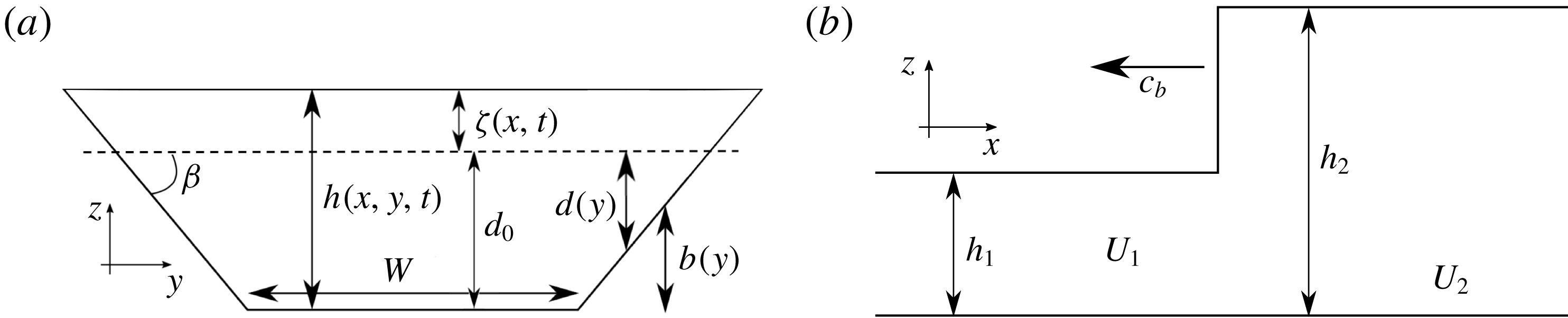
The geometry of the channel is represented by the bathymetry sketched in figure 7. Width
 $W$
, angle
 $\unicode[STIX]{x1D6FD}$
and water depth
 $h_{1}$
are the same as in Treske (Reference Treske1994):
 $W=1.24$
m,
 $\tan \unicode[STIX]{x1D6FD}=1/3$
,
 $h_{1}=0.16$
m.
Bore propagation in a trapezoidal open channel. (a) Cross view; (b) lateral view. Definition of variables:
 $W$
; width of the channel,
 $h$
; water depth,
 $d_{0}$
; still water depth on the axis,
 $\unicode[STIX]{x1D6FD}$
; angle of the banks,
 $U$
; section-averaged velocity in the axis direction,
 $c_{b}$
; bore celerity.

The jump conditions required to initialize the computations are obtained from a section-integrated version of the shallow water equations (Chanson Reference Chanson2004):
 $$\begin{eqnarray}\left.\begin{array}{@{}c@{}}{\displaystyle \frac{\unicode[STIX]{x2202}A}{\unicode[STIX]{x2202}t}}+{\displaystyle \frac{\unicode[STIX]{x2202}Q}{\unicode[STIX]{x2202}x}}=0,\\ {\displaystyle \frac{\unicode[STIX]{x2202}Q}{\unicode[STIX]{x2202}t}}+{\displaystyle \frac{\unicode[STIX]{x2202}}{\unicode[STIX]{x2202}x}}\left({\displaystyle \frac{Q^{2}}{A}}+K\right)=0,\end{array}\right\}\end{eqnarray}$$
where, as in figure 5(a),
 $d_{0}$
is a constant still water depth,
 $h_{0}=d_{0}+\unicode[STIX]{x1D701}(x,t)$
is the depth on the channel axis associated with a wave height
 $\unicode[STIX]{x1D701}$
constant along the section,
 $A=Wh_{0}+h_{0}^{2}/\text{tan}\,\unicode[STIX]{x1D6FD}$
is the wet section and
 $Q=UA$
is the total flow rate through the wet section. For the configuration of figure 5(a), following Chanson (Reference Chanson2004), the effective hydrostatic pressure
 $K$
can be easily shown to be
 $$\begin{eqnarray}K=g{\displaystyle \frac{Wh_{0}^{2}}{2}}+g{\displaystyle \frac{h_{0}^{3}}{3\tan \unicode[STIX]{x1D6FD}}}.\end{eqnarray}$$
The Rankine–Hugoniot relations become in this case:
 $$\begin{eqnarray}\left.\begin{array}{@{}c@{}}U_{1}-c_{b}=-\left(g{\displaystyle \frac{A_{2}}{A_{1}}}{\displaystyle \frac{K_{2}-K_{1}}{A_{2}-A_{1}}}\right)^{1/2},\\ U_{2}-c_{b}=-\left(g{\displaystyle \frac{A_{1}}{A_{2}}}{\displaystyle \frac{K_{2}-K_{1}}{A_{2}-A_{1}}}\right)^{1/2},\end{array}\right\}\end{eqnarray}$$
reducing to (2.3) for
 $\tan \unicode[STIX]{x1D6FD}\rightarrow \infty$
. We have performed simulations for different values of the Froude number defined as
 $$\begin{eqnarray}Fr={\displaystyle \frac{|U_{1}-c_{b}|}{\sqrt{g\overline{h}_{1}}}},\quad \overline{h}_{1}:={\displaystyle \frac{A_{1}}{\unicode[STIX]{x2202}_{h}A(h_{1})}}={\displaystyle \frac{W\tan \unicode[STIX]{x1D6FD}+h_{1}}{W\tan \unicode[STIX]{x1D6FD}+2h_{1}}}h_{1}.\end{eqnarray}$$
The computational domain is a rectangle of dimensions
 $[100\times 1.5]~\text{m}^{2}$
corresponding to half of the channel width. Symmetry/reflecting boundary conditions are imposed on the axis. The initial solution is defined by the following regularization of (3.3):
 $$\begin{eqnarray}\left.\begin{array}{@{}c@{}}h(x,y,t=0)={\displaystyle \frac{h_{2}-h_{1}}{2}}\tanh \left({\displaystyle \frac{x-x_{0}}{l_{t}}}\right)+h_{2}-b(y),\\ u(x,y,t=0)={\displaystyle \frac{U_{2}-U_{1}}{2}}\tanh \left({\displaystyle \frac{x-x_{0}}{l_{t}}}\right)+U_{2},\\ v(x,y,t=0)=0,\end{array}\right\}\end{eqnarray}$$
where
 $x_{0}=95$
m and
 $l_{t}=0.5$
m, and having assumed velocities to have a uniform value across the section. Grid sizes of
 $\unicode[STIX]{x1D6FF}_{x}=0.04$
m and
 $\unicode[STIX]{x1D6FF}_{y}=0.05$
m, respectively in the
 $x$
and
 $y$
directions, are used. These values guarantee at least approximately 20 points per wavelength for the shortest waves simulated, and has been verified to provide results which are practically mesh converged.
3.2 Numerical results
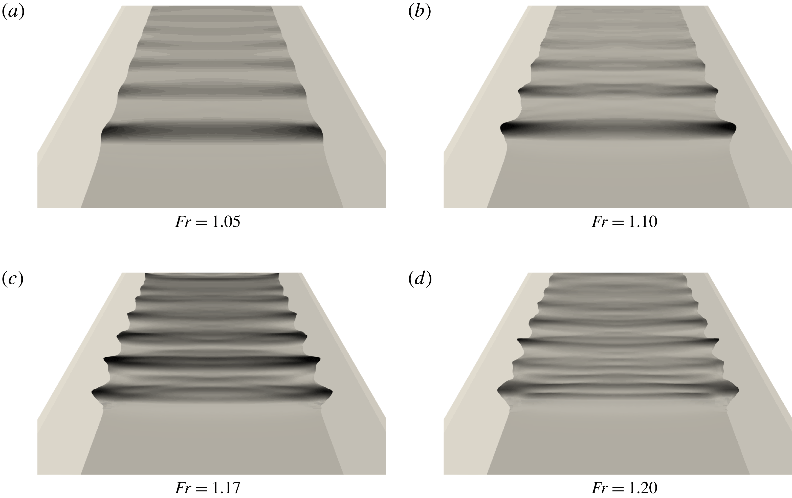
Snapshots of the simulated undular bores for different Froude numbers.

Simulations have been performed for a range of Froude numbers from 1.02 to 1.275, a range sufficiently large to study the LFN–HFN transition, while remaining well below the second transition to a fully breaking bore along the channel axis. Snapshots of the water levels obtained for four representative values of
 $Fr$
are reported in figure 8. Compared to the visualization of figure 3, these pictures show the complexity of the wave dynamics induced by the interaction with the sloping banks. The low Froude results look somewhat more similar to the results obtained for a rectangular section, with a wave phase structure uniform along the section. As
 $Fr$
increases the wave field becomes highly two-dimensional.
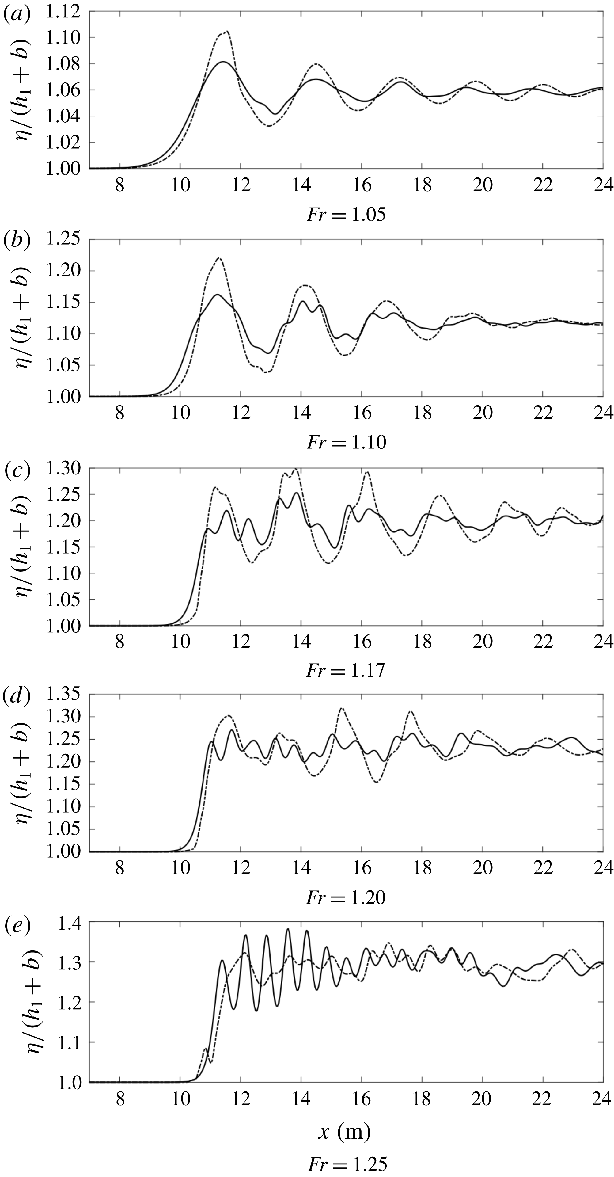
Free surface profiles for different Froude numbers. Continuous line: axis. Dash-dot: banks.

To further investigate this point, we have reported in figure 9 the free surface elevation along the channel axis and close to the banks. These figures show clearly the transition between the LFN regime, with uniform phase structure along the section and a single dominant wavelength (figure 9 a,b), to the HFN regime in which two types of waves interact (figure 9 c–e). The interaction between these two leads to the two-dimensional wave fields of the bottom pictures in figure 8. As in the field observations by Bonneton et al. (Reference Bonneton, Bonneton, Parisot and Castelle2015), and as discussed in the introduction, the LFN regime is characterized by amplitudes being higher on the banks than on the axis, while the HFN bores have larger amplitudes on the channel axis. We underline in particular the striking resemblance of the HFN bore of figure 9(e) and of the LFN wave of figure 9(a), with the bores measured in the Garonne river and reported respectively in figures 2(b) and 2(d).
To provide a more quantitative assessment of the numerical results, we have post processed the time series of the water elevation for all the simulated values of
 $Fr$
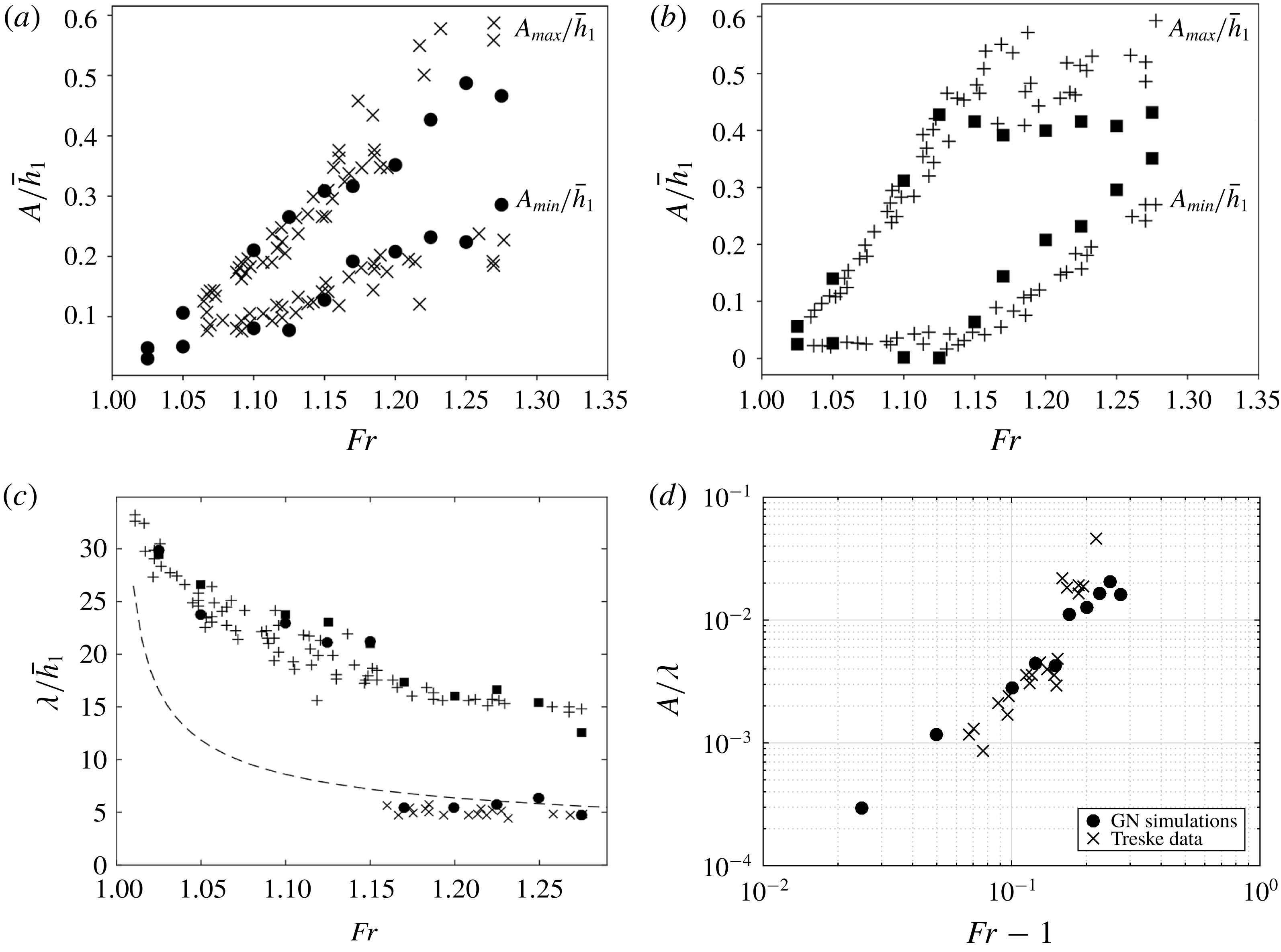
to obtain the amplitude of the first peak and trough, the wavelength and the steepness. The results are compared to the experimental data by Treske (Reference Treske1994) in figure 10.
Wavelength and water level of undular bores in a channel with trapezoidal section. (a) Water elevation (axis), (b) water elevation (banks), (c) wavelength, (d) steepness (axis).
 $\times$
: Data of Treske (Reference Treske1994) axis,
 $+$
: data of Treske (Reference Treske1994) banks, ●: simulated values on the channel axis, ▪: simulated values on the banks, — —: Lemoine (Reference Lemoine1948) theory.

The numerical peak and trough amplitude, denoted by
 $A_{max}$
and
 $A_{min}$
respectively, are compared to the experiments in figures 10(a) for the channel axis, and 10(b) for the sloping banks. On the axis both experiments and simulations show a quasi-linear increase in the water elevations with the Froude number, with no clear transition. On the contrary, on the sloping banks we observe a clear transition, taking place for a value
 $Fr_{t}\approx 1.15$
. Before
 $Fr_{t}$
, the peak elevations increase more rapidly than on the axis, in agreement with the LFN signals observed in figures 9(a) and 2(d). In the LFN regime, the trough amplitudes
 $A_{min}$
remain roughly constant. After the transition, on the sloping banks the increase of peak amplitude with
 $Fr$
becomes very weak, while the trough amplitude starts increasing. This leads to the HFN regime in which the amplitudes on the axis are more important than those on the sloping banks, as already observed in figures 9(e) and 2(b) for the field measurements. The agreement between simulations and experiment is very good, with the exception of a small advance on the onset of the transition, and of a slight underestimation of the slow growth of the peaks after
 $Fr_{t}$
, which can be seen in figure 10(b). This mismatch is most likely related to the parametrization of the wave breaking closure for which we have used standard values from Kazolea et al. (Reference Kazolea, Delis and Synolakis2014), and did not try to optimize.
The transition between the LFN and HFN bores can be seen very clearly in the wavelength and steepness distributions, reported in figures 10(c) and 10(d) respectively. For these quantities the agreement between simulations and experimental data is excellent. We can see that the HFN regime is characterized by wavelengths on the axis very close to those observed in straight channels. This is made more clear by reporting in the figure the values computed by means of the theory by Lemoine (Reference Lemoine1948). The curve provides a very good fit of the wavelengths observed in the simulations and in the experiments. This suggests that non-hydrostatic dispersive effects are the dominating ones on the channel axis, as in Favre waves. On the sloping banks some other phenomenon is active, as the wavelengths observed are approximately three times larger than on the axis. This leads to wave signals like those reported in figures 9(c) and 9(d). Below
 $Fr_{t}$
both on the axis and on the sloping banks wavelengths have values three or four times larger than those predicted by the theory of Lemoine (Reference Lemoine1948). In the LFN regime, the trend with the Froude number is the same as observed on the banks for HFN waves. The distribution of the steepness
 $(A_{max}-A_{min})/2\unicode[STIX]{x1D706}$
on the channel axis, reported for completeness in figure 10(d), also shows the transition between the LFN and HFN waves. Very similar results with field data from the Garonne and Seine river field measurements can be found in Bonneton et al. (Reference Bonneton, Bonneton, Parisot and Castelle2015). It should be remarked that the separation between the two regimes is not abrupt. Although the difference is very clear when looking at Froude numbers sufficiently above and below
 $Fr_{t}$
, when approaching this value things are less definite, as one can start guessing from figure 9(c) for example. So one should speak rather of a narrow transition region, roughly centred on
 $Ft_{t}=1.15$
for the geometry considered here.
Our results show clearly that the LFN–HFN transition can be described satisfactorily by simulations based on weakly dispersive Serre–Green–Naghdi models, with a very good overall agreement between simulations and experiments. The main question remaining open is the origin of the LFN bores. The objective of the remainder of this paper is to propose a dispersive-like mechanism for these waves.
4 Dispersive-like mechanism for small Froude numbers
4.1 Motivation
This section discusses one of the main results of this paper. We will show that the dispersion characteristics of LFN waves can be modelled by a fully hydrostatic section-averaged model, obtained starting from the shallow water equations. The dispersive effects embedded in this model are purely hydrostatic and related to the refraction along the banks. For this reason we speak of a dispersive-like process.
Note that waves with characteristics somewhat similar to those observed here are the well-known edge waves for which there exist a certain number of analytical solutions obtained from the full potential equations. The interested reader may consult for example the works of Ursell (Reference Ursell1952), Miles (Reference Miles1989) and more recently Johnson (Reference Johnson2007), and references therein.
As in the case of edge waves, we claim that the main physical mechanism acting here is the refraction induced by the sloping banks. To give a theoretical characterization of the LFN waves here we claim that we can start from an appropriately scaled linearized shallow water approximation. Indeed, dispersive propagation has been shown to arise for standard linear waves in heterogeneous media (Quezada de Luna & Ketcheson Reference Quezada de Luna and Ketcheson2013; Ketcheson & Quezada de Luna Reference Ketcheson and Quezada de Luna2015). For the application considered here, our intuition is related to two observations. First, the LFN waves are much longer than the standard Favre waves. Second, in the HFN regime these waves can still be observed in trapezoidal channels on the sloping banks where the non-hydrostatic effects are known to be less relevant. To verify this intuition, we propose a first experiment consisting of repeating the simulations of § 3 with the shallow water equations. The results are summarized in figure 11. The left picture in the figure shows the free surface profile obtained numerically for
 $Fr=1.05$
. The presence of undulations in the propagation is clearly visible. Also, these features do not disappear as the mesh is refined. The right picture in the figure shows the comparison of the wavelengths measured in the shallow water simulations with the data of Treske. The hydrostatic model clearly reproduces the LFN waves. Also note that the wavelengths measured are the same on the banks and on the axis, as one would expect.
Numerical verification: Treske experiments reproduced with shallow water simulations. (a) Free surface for
 $Fr=1.15$
. (b) Comparison of computed wavelengths (▴) with the data from the experiment by Treske (
 $+$
: banks,
 $\times$
: axis).

To complete the study, in the following we discuss an asymptotic and section-averaged approximation of the linear hydrostatic shallow water equations exhibiting geometrical dispersion. To obtain this result we make the hypothesis that a fast wave refraction phenomenon is present in the transversal direction. The time scale associated with this phenomenon, denoted by
 $\unicode[STIX]{x1D70F}_{y}$
is thus assumed to be much smaller than the time scale in the propagation direction, denoted by
 $\unicode[STIX]{x1D70F}_{x}$
. This hypothesis implies the existence of a small parameter defined as the ratio between the transversal and longitudinal time scales or, equivalently, as the reference length ratio
 $$\begin{eqnarray}\unicode[STIX]{x1D6FF}:={\displaystyle \frac{\unicode[STIX]{x1D70F}_{y}}{\unicode[STIX]{x1D70F}_{x}}}\approx {\displaystyle \frac{L_{y}}{L_{x}}}\ll 1.\end{eqnarray}$$
The correctness of our asymptotic approximation is first verified against numerical computations of monochromatic waves, and finally applied to the experiments of Treske by means of an analysis similar to the one performed in Lemoine (Reference Lemoine1948).
4.2 Hydrostatic section-averaged approximation
Main geometrical notation for the asymptotic analysis. (a) Cross-section; (b) side view.

Consider the geometrical configuration depicted in figure 12. We are interested in deriving a linear approximate model for the evolution of the section-averaged free surface, where the section-averaging operator is denoted by an overline, and defined by
 $$\begin{eqnarray}\overline{(\cdot )}={\displaystyle \frac{1}{2y_{0}}}\int _{-y_{0}}^{y_{0}}(\cdot )\,\text{d}y.\end{eqnarray}$$
An exception to the above notation is the section-averaged depth at still water, which we denote by
 $h_{0}$
. Using the notation of figure 12, we have that
 $$\begin{eqnarray}h_{0}=\overline{d}=d_{0}-\overline{b}.\end{eqnarray}$$
We also denote by
 $C_{0}^{2}=gh_{0}$
the square celerity corresponding to
 $h_{0}$
. Let now
 $L_{y}$
be the half-channel breadth at the still water level,
 $a$
a reference wave height and
 $\unicode[STIX]{x1D716}=a/h_{0}$
the standard nonlinearity parameter. We consider the following dimensionless form of the main physical variables (cf. figure 12):
 $$\begin{eqnarray}\left.\begin{array}{@{}c@{}}\unicode[STIX]{x2202}x^{\prime }={\displaystyle \frac{\unicode[STIX]{x2202}x}{L_{x}}},\quad \unicode[STIX]{x2202}y^{\prime }={\displaystyle \frac{\unicode[STIX]{x2202}y}{L_{y}}},\\ b^{\prime }={\displaystyle \frac{b}{h_{0}}},\quad \unicode[STIX]{x1D701}^{\prime }={\displaystyle \frac{\unicode[STIX]{x1D701}}{a}},\quad d^{\prime }={\displaystyle \frac{d}{h_{0}}},\\ t^{\prime }={\displaystyle \frac{C_{0}}{L_{x}}}t,\quad u^{\prime }={\displaystyle \frac{u}{\unicode[STIX]{x1D716}C_{0}}},\quad v^{\prime }={\displaystyle \frac{v}{\unicode[STIX]{x1D716}C_{0}}}.\end{array}\right\}\end{eqnarray}$$
In the above equations we recall that
 $u$
and
 $v$
denote the components of the depth-averaged flow speed for which the dimensional scaling by
 $\unicode[STIX]{x1D716}C_{0}$
is a classical choice (see e.g. Dingemans Reference Dingemans1997; Lannes Reference Lannes2013). The quantity
 $y_{0}$
, required for the evaluation of the section average, is the actual time-/space-dependent half-breadth corresponding to the local position of the water line. This means that
 $$\begin{eqnarray}y_{0}=\left.L_{y}+\int _{0}^{t}v\right|_{y=y_{0}},\,\text{d}t\rightarrow y_{0}^{\prime }=1+{\displaystyle \frac{\unicode[STIX]{x1D716}}{\unicode[STIX]{x1D6FF}}}\unicode[STIX]{x1D6E5}_{y},\quad \unicode[STIX]{x1D6E5}_{y}:=\left.\int _{0}^{t\prime }v^{\prime }\right|_{y^{\prime }=y_{0}^{\prime }}\,\text{d}t^{\prime }.\end{eqnarray}$$
We now consider the nonlinear shallow water equations in dimensionless form
 $$\begin{eqnarray}\left.\begin{array}{@{}c@{}}\unicode[STIX]{x2202}_{t}\unicode[STIX]{x1D701}+\unicode[STIX]{x2202}_{x}((d+\unicode[STIX]{x1D716}\unicode[STIX]{x1D701})u)+{\displaystyle \frac{1}{\unicode[STIX]{x1D6FF}}}\unicode[STIX]{x2202}_{y}((d+\unicode[STIX]{x1D716}\unicode[STIX]{x1D701})v)=0,\\ \unicode[STIX]{x2202}_{t}u+\unicode[STIX]{x1D716}u\unicode[STIX]{x2202}_{x}u+{\displaystyle \frac{\unicode[STIX]{x1D716}}{\unicode[STIX]{x1D6FF}}}v\unicode[STIX]{x2202}_{y}u+\unicode[STIX]{x2202}_{x}\unicode[STIX]{x1D701}=0,\\ \unicode[STIX]{x2202}_{t}v+\unicode[STIX]{x1D716}u\unicode[STIX]{x2202}_{x}v+{\displaystyle \frac{\unicode[STIX]{x1D716}}{\unicode[STIX]{x1D6FF}}}v\unicode[STIX]{x2202}_{y}v+{\displaystyle \frac{1}{\unicode[STIX]{x1D6FF}}}\unicode[STIX]{x2202}_{y}\unicode[STIX]{x1D701}=0.\end{array}\right\}\end{eqnarray}$$
Note that the primes have been dropped to simplify the notation. For simplicity we assume that the flow is fully symmetric with respect to the channel centreline
 $y=0$
. On the banks, the equations satisfy the boundary conditions
 $$\begin{eqnarray}\pm y=y_{0}+{\displaystyle \frac{\unicode[STIX]{x1D716}}{\unicode[STIX]{x1D6FF}}}\unicode[STIX]{x1D6E5}_{y}\Rightarrow (d+\unicode[STIX]{x1D716}\unicode[STIX]{x1D701})v=0,\quad (d+\unicode[STIX]{x1D716}\unicode[STIX]{x1D701})u=0,\quad d+\unicode[STIX]{x1D716}\unicode[STIX]{x1D701}=0.\end{eqnarray}$$
The condition on
 $(d+\unicode[STIX]{x1D716}\unicode[STIX]{x1D701})v$
also applies to channels with vertical side walls.
We now pass to a fully linear regime
 $\unicode[STIX]{x1D716}\rightarrow 0$
. Equation (4.5) can be used to simplify the domain definition in the transversal direction which is now
 $y\in [-1,1]$
. This leads to a simplification of the section-averaging operator which becomes
 $$\begin{eqnarray}\overline{(\cdot )}={\displaystyle \frac{1}{2}}\int _{-1}^{1}(\cdot )\,\text{d}y.\end{eqnarray}$$
The linearized model equations read
 $$\begin{eqnarray}\left.\begin{array}{@{}c@{}}\unicode[STIX]{x2202}_{t}\unicode[STIX]{x1D701}+\text{d}\unicode[STIX]{x2202}_{x}u+{\displaystyle \frac{1}{\unicode[STIX]{x1D6FF}}}\unicode[STIX]{x2202}_{y}(\text{d}v)=0,\\ \unicode[STIX]{x2202}_{t}u+\unicode[STIX]{x2202}_{x}\unicode[STIX]{x1D701}=0,\\ \unicode[STIX]{x2202}_{t}v+{\displaystyle \frac{1}{\unicode[STIX]{x1D6FF}}}\unicode[STIX]{x2202}_{y}\unicode[STIX]{x1D701}=0,\\ y=\pm 1\rightarrow \text{d}v=0,\end{array}\right\}\end{eqnarray}$$
where the last expression is a linear non-dimensional boundary condition, still valid for both banks and vertical side walls.
The boundary condition in (4.9) can be readily used to derive a section-averaged wave equation by taking the average of the first equation in (4.9):
 $$\begin{eqnarray}\left.\begin{array}{@{}c@{}}\unicode[STIX]{x2202}_{t}\overline{\unicode[STIX]{x1D701}}+\overline{\text{d}\unicode[STIX]{x2202}_{x}u}=0\\ \unicode[STIX]{x2202}_{t}u+\unicode[STIX]{x2202}_{x}\unicode[STIX]{x1D701}=0\end{array}\right\}\Rightarrow \unicode[STIX]{x2202}_{tt}\overline{\unicode[STIX]{x1D701}}-\overline{\text{d}\unicode[STIX]{x2202}_{xx}\unicode[STIX]{x1D701}}=0.\end{eqnarray}$$
Our objective is to obtain a closed form of the above equation for the evolution in space and time of
 $\overline{\unicode[STIX]{x1D701}}$
. To this end we invoke hypothesis (4.1), and we introduce asymptotic expansions of all the variables in terms of the small parameter
 $\unicode[STIX]{x1D6FF}$
:
 $$\begin{eqnarray}\left.\begin{array}{@{}c@{}}\unicode[STIX]{x1D701}=\unicode[STIX]{x1D701}_{0}+\unicode[STIX]{x1D6FF}\unicode[STIX]{x1D701}_{1}+\unicode[STIX]{x1D6FF}^{2}\unicode[STIX]{x1D701}_{2}+\cdots \,,\\ u=u_{0}+\unicode[STIX]{x1D6FF}u_{1}+\unicode[STIX]{x1D6FF}^{2}u_{2}+\cdots \,,\\ v=v_{0}+\unicode[STIX]{x1D6FF}v_{1}+\unicode[STIX]{x1D6FF}^{2}v_{2}+\cdots \,.\end{array}\right\}\end{eqnarray}$$
These expansions are substituted in (4.9), and terms of equal powers in
 $\unicode[STIX]{x1D6FF}$
are equated. This results in a system of partial differential relations/equations for the coefficients in the development. This system can be closed by applying iteratively the three following steps:
(i)
 $\unicode[STIX]{x2202}_{y}(\text{d}v_{n+1})=-(\unicode[STIX]{x2202}_{t}\unicode[STIX]{x1D701}_{n}+\text{d}\unicode[STIX]{x2202}_{x}u_{n})$
, with
$\text{d}v_{n+1}=0$
for
$y=\pm 1$
;
(ii)
$\unicode[STIX]{x2202}_{t}u_{n}=-\unicode[STIX]{x2202}_{x}\unicode[STIX]{x1D701}_{n}$
,
$\forall \,n$
;(iii)
$\unicode[STIX]{x2202}_{y}\unicode[STIX]{x1D701}_{n+1}=-\unicode[STIX]{x2202}_{t}v_{n}$
.


To complete the procedure, we need a starting condition as well as a way of closing the integration along
 $y$
required in step (iii) (for step (i) the boundary condition provides this closure).
The starting condition is obtained by observing that
 $\unicode[STIX]{x2202}_{y}(\text{d}v_{0})=0$
with
 $\text{d}v_{0}=0$
on both sides of the domain. This implies
 $v_{0}=0$
which is used as initial value in (i) and (iii).
Concerning step (iii), the closure used here is based on the explicit computation of a primitive function
 $Z_{n+1}$
such that
 $\unicode[STIX]{x2202}_{y}Z_{n+1}=-\unicode[STIX]{x2202}_{t}v_{n}$
. This means that
 $$\begin{eqnarray}\unicode[STIX]{x1D701}_{n+1}=Z_{n+1}+F(x,t).\end{eqnarray}$$
Note that in general
 $Z_{n+1}=Z_{n+1}(x,y,t)$
. We express the integration ‘constant’
 $F$
using section-averaged values:
 $F=\overline{\unicode[STIX]{x1D701}}_{n+1}-\overline{Z}_{n+1}$
. This gives the closure for step (iii):
 $$\begin{eqnarray}\unicode[STIX]{x1D701}_{n+1}=\overline{\unicode[STIX]{x1D701}}_{n+1}+Z_{n+1}-\overline{Z}_{n+1}.\end{eqnarray}$$
Applying this procedure we obtain the following order results.
- Order 0
- (4.14)$$\begin{eqnarray}\left.\begin{array}{@{}c@{}}v_{0}=0,\\ \unicode[STIX]{x1D701}_{0}=\overline{\unicode[STIX]{x1D701}}_{0}(x,t).\end{array}\right\}\end{eqnarray}$$
- Order 1
- (4.15)$$\begin{eqnarray}\left.\begin{array}{@{}c@{}}\displaystyle v_{1}=-{\displaystyle \frac{1+y}{d}}\unicode[STIX]{x2202}_{t}\overline{\unicode[STIX]{x1D701}}_{0}-{\displaystyle \frac{D}{d}}\unicode[STIX]{x2202}_{x}\overline{u}_{0},\quad D=\int _{-1}^{y}d(s)\,\text{d}s,\\ \unicode[STIX]{x1D701}_{1}=\overline{\unicode[STIX]{x1D701}}_{1}(x,t).\end{array}\right\}\end{eqnarray}$$
- Order 2
- (4.16)$$\begin{eqnarray}\left.\begin{array}{@{}c@{}}\displaystyle v_{2}=-{\displaystyle \frac{1+y}{d}}\unicode[STIX]{x2202}_{t}\overline{\unicode[STIX]{x1D701}}_{1}-{\displaystyle \frac{D}{d}}\unicode[STIX]{x2202}_{x}\overline{u}_{1},\quad D=\int _{-1}^{y}d(s)\unicode[STIX]{x2202}s,\\ \displaystyle \unicode[STIX]{x1D701}_{2}=\overline{\unicode[STIX]{x1D701}}_{2}(x,t)+(\unicode[STIX]{x1D705}(y)-\overline{\unicode[STIX]{x1D705}})\unicode[STIX]{x2202}_{xx}\overline{\unicode[STIX]{x1D701}}_{0},\quad \unicode[STIX]{x1D705}(y)=\int _{-1}^{y}{\displaystyle \frac{1+s-D(s)}{d(s)}}\,\text{d}s.\end{array}\right\}\end{eqnarray}$$
- Order 3
- (4.17)$$\begin{eqnarray}\left.\begin{array}{@{}c@{}}\displaystyle v_{3}=-{\displaystyle \frac{1}{d}}\int _{-1}^{y}(\unicode[STIX]{x2202}_{t}\unicode[STIX]{x1D702}_{2}+\text{d}\unicode[STIX]{x2202}_{x}u_{2})\unicode[STIX]{x2202}s,\\ \displaystyle \unicode[STIX]{x1D701}_{3}=\overline{\unicode[STIX]{x1D701}}_{3}(x,t)+(\unicode[STIX]{x1D705}(y)-\overline{\unicode[STIX]{x1D705}})\unicode[STIX]{x2202}_{xx}\overline{\unicode[STIX]{x1D701}}_{1},\quad \unicode[STIX]{x1D705}(y)=\int _{-1}^{y}{\displaystyle \frac{1+s-D(s)}{d(s)}}\,\text{d}s.\end{array}\right\}\end{eqnarray}$$


We do not proceed further as the above solutions provide an approximation which is exact within
 $O(\unicode[STIX]{x1D6FF}^{4})$
. This is the typical order retained for weakly dispersive models such as e.g. the Serre–Green–Naghdi model used in this paper. Collecting all the orders, we have
 $$\begin{eqnarray}\unicode[STIX]{x1D701}=\overline{\unicode[STIX]{x1D701}}_{0}+\unicode[STIX]{x1D6FF}\overline{\unicode[STIX]{x1D701}}_{1}+\unicode[STIX]{x1D6FF}^{2}(\overline{\unicode[STIX]{x1D701}}_{2}+(\unicode[STIX]{x1D705}(y)-\overline{\unicode[STIX]{x1D705}})\unicode[STIX]{x2202}_{xx}\overline{\unicode[STIX]{x1D701}}_{0})+\unicode[STIX]{x1D6FF}^{3}(\overline{\unicode[STIX]{x1D701}}_{3}+(\unicode[STIX]{x1D705}(y)-\overline{\unicode[STIX]{x1D705}})\unicode[STIX]{x2202}_{xx}\overline{\unicode[STIX]{x1D701}}_{1})+O(\unicode[STIX]{x1D6FF}^{4}).\end{eqnarray}$$
Using the relations
 $\unicode[STIX]{x1D701}=\unicode[STIX]{x1D701}_{0}+\unicode[STIX]{x1D6FF}\unicode[STIX]{x1D701}_{1}+O(\unicode[STIX]{x1D6FF}^{2})$
and
 $\overline{\unicode[STIX]{x1D701}}_{0}+\unicode[STIX]{x1D6FF}\overline{\unicode[STIX]{x1D701}}_{1}+\unicode[STIX]{x1D6FF}^{2}\overline{\unicode[STIX]{x1D701}}_{2}+\unicode[STIX]{x1D6FF}^{3}\overline{\unicode[STIX]{x1D701}}_{3}=\overline{\unicode[STIX]{x1D701}}+O(\unicode[STIX]{x1D6FF}^{4})$
, we deduce the following asymptotic expansion for the free surface:
 $$\begin{eqnarray}\unicode[STIX]{x1D701}=\overline{\unicode[STIX]{x1D701}}+\unicode[STIX]{x1D6FF}^{2}(\unicode[STIX]{x1D705}(y)-\overline{\unicode[STIX]{x1D705}})\unicode[STIX]{x2202}_{xx}\overline{\unicode[STIX]{x1D701}}+O(\unicode[STIX]{x1D6FF}^{4}).\end{eqnarray}$$
We can now use this expansion in the section-averaged wave equation (4.10) to obtain, within an
 $O(\unicode[STIX]{x1D6FF}^{4})$
error, the following section-averaged dispersive approximation:
 $$\begin{eqnarray}\unicode[STIX]{x2202}_{tt}\overline{\unicode[STIX]{x1D701}}-\unicode[STIX]{x2202}_{xx}\overline{\unicode[STIX]{x1D701}}-\unicode[STIX]{x1D6FF}^{2}\unicode[STIX]{x1D712}\unicode[STIX]{x2202}_{xxxx}\overline{\unicode[STIX]{x1D701}}=0.\end{eqnarray}$$
The coefficient
 $\unicode[STIX]{x1D712}$
is a geometrical dispersion coefficient defined by
 $$\begin{eqnarray}\unicode[STIX]{x1D712}=\overline{d(y)\unicode[STIX]{x1D705}(y)}-\overline{d}\,\overline{\unicode[STIX]{x1D705}},\end{eqnarray}$$
with the expression for
 $\unicode[STIX]{x1D705}(y)$
provided both in (4.16) and (4.17). We stress that this dispersive perturbation is only related to the geometrical shape of the channel section, and to the initial hypothesis that
 $\unicode[STIX]{x1D6FF}\ll 1$
. We recall that this hypothesis implies that the transversal time/length scale, related to the wave refraction, is much smaller than the time/length scale in the main propagation direction.
By means of standard Fourier transform, we can easily obtain the dispersion relation verified by solutions of (4.20), which reads in dimensional form
 $$\begin{eqnarray}\unicode[STIX]{x1D714}^{2}=k^{2}C_{0}^{2}(1-\unicode[STIX]{x1D712}(kL_{y})^{2}),\end{eqnarray}$$
with
 $k$
the wavenumber.
4.3 Numerical verification of the expansion for monochromatic waves
Our first objective is to verify the asymptotic approximation obtained. This is not a completely trivial task, as we do not have any analytical reference to compare to. To perform this verification, we compare the dispersion characteristics of the asymptotic model to those obtained numerically on fine meshes with the code described in § 2.1 in the shallow water limit.
Setting
 $\overline{\unicode[STIX]{x1D701}}=a\sin (kx-\unicode[STIX]{x1D714}t)$
we can deduce for a given channel a
 $y$
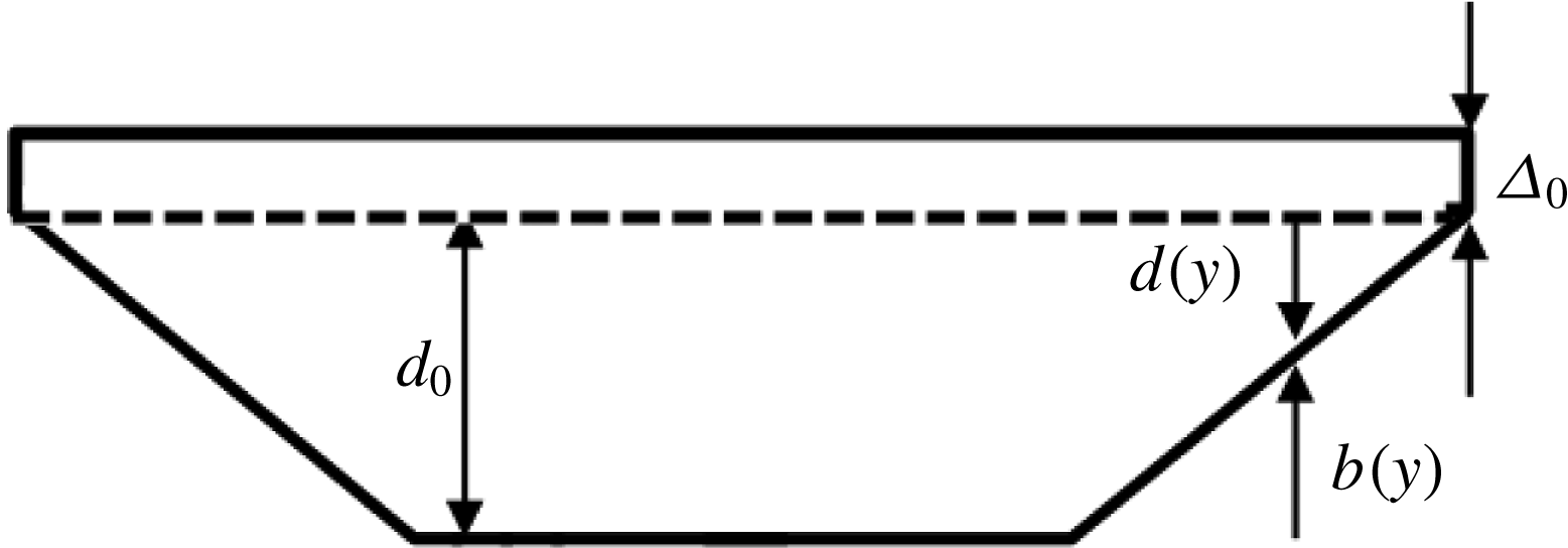
-dependent boundary condition from (4.19). This is used as an inlet condition in the code. To avoid the impact of the treatment of the wet–dry interface, in the computations the bathymetry is modified by introducing vertical lateral walls, as depicted in figure 13. Note that, as remarked several times, this configuration is also compatible with the boundary condition used in the asymptotic development. The computations are started from a flat free surface, and the inlet boundary condition is propagated numerically in the channel. The numerical solution obtained is then averaged over the section and the resulting signal analysed to measure the dispersion relation provided by the simulations. Note that these results embed full nonlinearity and a full approximation of the transverse propagation. For this reason they are considered as a good reference against which the theoretical relation (4.22) can be tested.
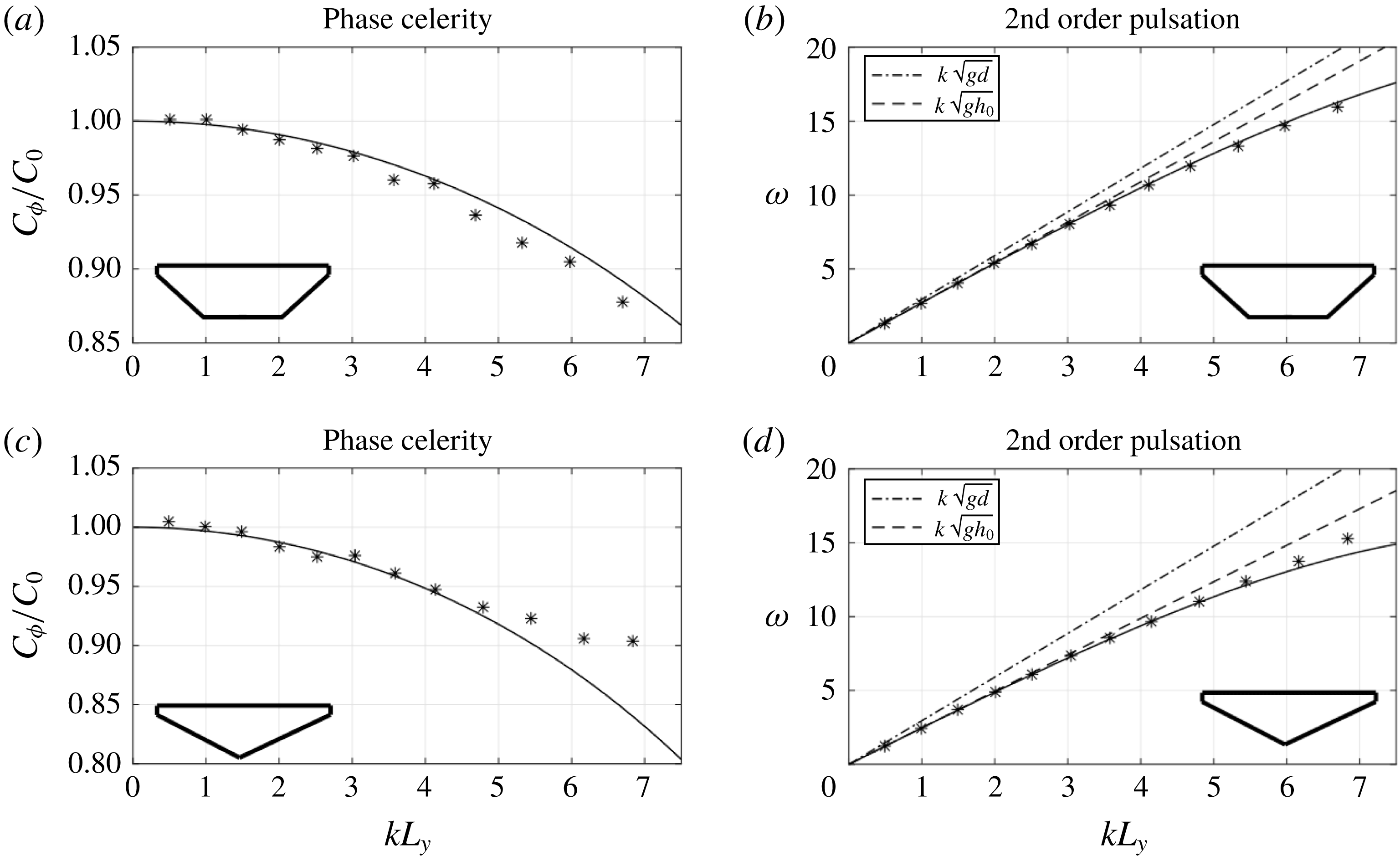
The resulting comparisons are reported in figure 14 for trapezoidal and triangular channels in terms of non-dimensional celerity and phase. The figure highlights two things. First, a dispersive process is indeed present in the shallow water results. Secondly, for long waves, namely
 $kL_{y}\leqslant 5{-}6$
, the asymptotic approximation provides an excellent prediction of the physical dispersion relation. This confirms the soundness of the asymptotic development, and implicitly confirms the geometrical origin and hydrostatic nature of the dispersive behaviour observed. For this reason we speak here of dispersive-like waves, because actual physical non-hydrostatic/dispersive effects are not the origin of these waves.
Concerning the deviation observed for higher wavenumbers for the triangular shape may be related to the effects neglected in the asymptotic development (e.g. some geometrical nonlinearity to account for higher bank slopes).
Channel geometry used for the numerical verification.

Verification of the asymptotic analysis: trapezoidal (a,b) and triangular (c,d) section. (a,c) Celerity. (b,d) Phase.
 $\ast$
: shallow water code; ——: new asymptotic theory; – – –: linear phase for
 $d(y)=\overline{d}$
; — ⋅ —: linear phase for
 $d(y)=d_{0}$
.

4.4 Application to LFN bores
We propose here a method to predict the wavelength observed in the LFN regime in the spirit of Lemoine (Reference Lemoine1948). Using the linearized dispersive model derived in the previous sections, we compute theoretical wavelengths by equating the bore speed obtained from the jump conditions (3.3) with the celerity in (4.22):
 $$\begin{eqnarray}C_{0}^{2}(1-\unicode[STIX]{x1D712}(kL_{y})^{2})=g{\displaystyle \frac{A_{1}}{A_{2}}}{\displaystyle \frac{K_{2}-K_{1}}{A_{2}-A_{1}}}.\end{eqnarray}$$
For a given Froude number, the above equation can be readily solved for the wavelength
 $\unicode[STIX]{x1D706}=2\unicode[STIX]{x03C0}/k$
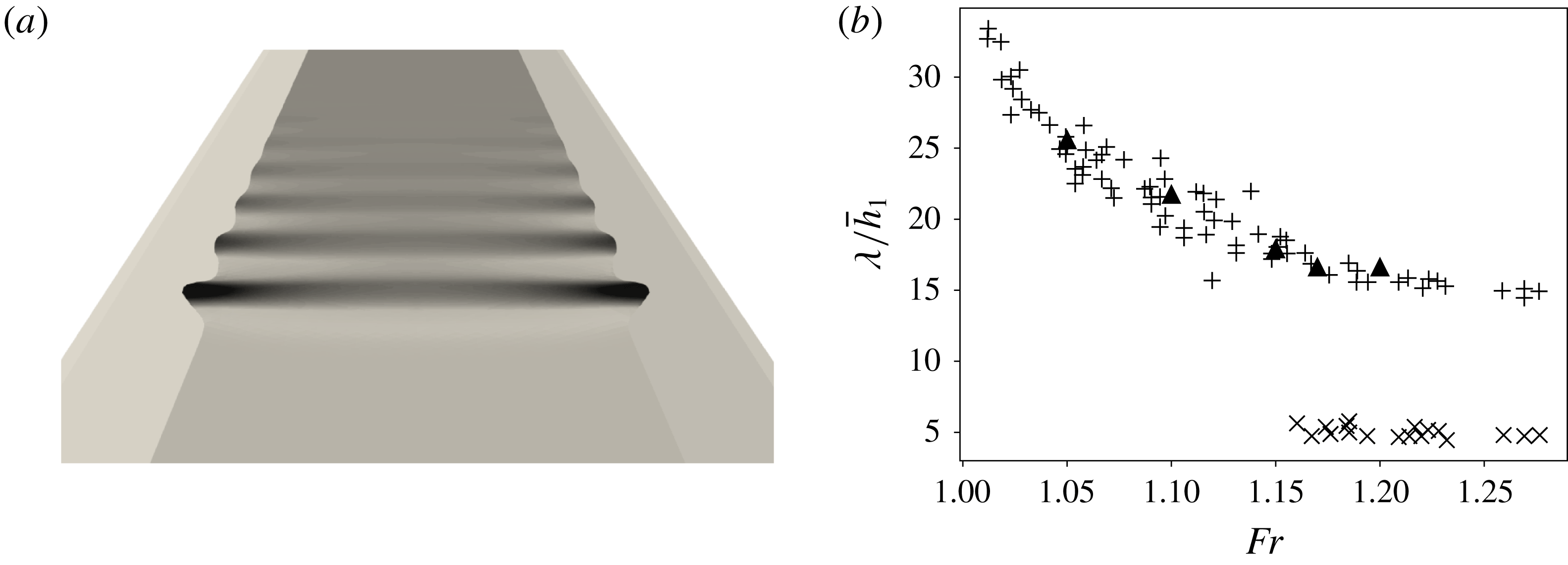
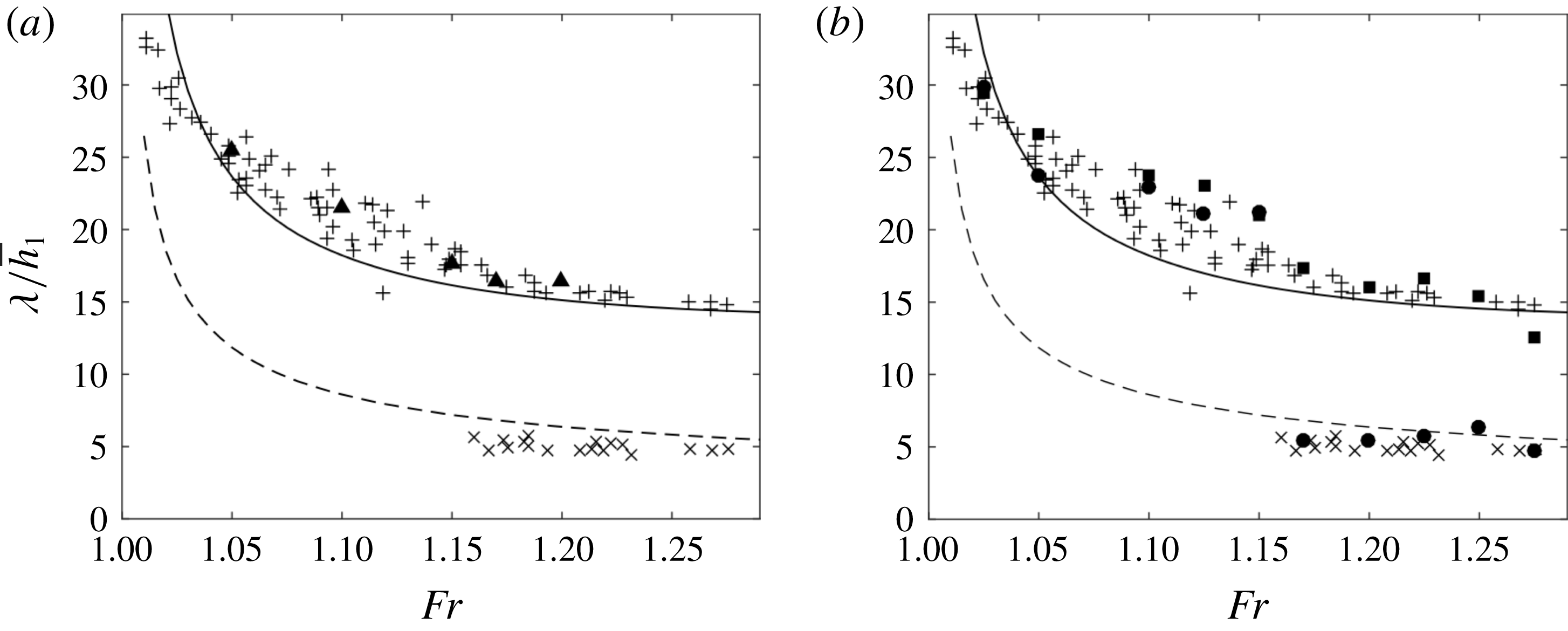
. The resulting wavelength distribution with respect to the Froude number is plotted in figure 15 against both the data by Treske, and the shallow water (a) and Serre–Green–Naghdi (b) simulations.
The results clearly shows that our theoretical analysis fully captures the nature of the LFN waves. They confirm that the low Froude waves observed in the experimental setting by Treske (Reference Treske1994), and those of the field measurements by Bonneton et al. (Reference Bonneton, Bonneton, Parisot and Castelle2015) have an entirely different nature from the so called Favre waves. The latter are associated with fully non-hydrostatic dispersion, while LFN bores are mainly related to the coupling of geometrical refraction in the transversal direction and hydrostatic wave propagation.
Theoretical wavelengths compared to numerical and experimental data. (a) Shallow water simulations; (b) Serre–Green–Naghdi simulations.
 $\times$
: data of Treske (Reference Treske1994) axis,
 $+$
: data of Treske (Reference Treske1994) banks, ●: Serre–Green–Naghdi simulations axis, ▪: Serre–Green–Naghdi simulations banks, ▴: shallow water simulations, — —: (Lemoine Reference Lemoine1948) theory, ——: new asymptotic theory.

5 Conclusions and outlook
In this paper we have proposed a detailed analysis of undular bore dynamics in channels of variable cross-section. By means of a weakly dispersive Serre–Green–Naghdi numerical model we have successfully reproduced the two undular bore regimes, a low Froude number (LFN) and a high Froude number (HFN) one, observed both in the experiments by Treske (Reference Treske1994) and in Bonneton et al. (Reference Bonneton, Bonneton, Parisot and Castelle2015) in field measurements in the Garonne and Seine rivers. In the HFN regime two families of waves are observed. On the channel axis there are short waves with characteristics similar to those of the well-known Favre waves. These are associated with non-hydrostatic dispersive effects. On the sloping banks, longer waves are observed, clearly not generated by the same phenomenon. The interaction between these two leads to a complex two-dimensional wave phase structure. In the LFN regime, only the long waves are observed in the whole channel. This gives a quasi-one-dimensional wave phase structure, with larger amplitudes on the banks. A dispersive-like mechanism related to geometrical refraction on the banks has been proposed as the phenomenon responsible for the LFN waves. The claim has been first verified numerically, showing that these waves can be reproduced with shallow water simulations. Then we have shown that, under the hypothesis that the time scale associated with refraction in the transversal direction is much smaller than the time scale associated with wave propagation, the section averaged free surface level verifies a linear dispersive wave equation. The corresponding dispersion relation has been used to compute theoretical wavelengths for the secondary waves which fit very accurately the wavelengths observed experimentally and numerically in the LFN regime.
This study clarifies the main mechanism active in the LFN regime. However, it remains to understand what the mechanisms are leading the transition between LFN and HFN waves. It will also be interesting to understand the dependence of the LFN waves on the geometrical parameters of the channel. Preliminary investigations have shown that wavelengths in the LFN regime decrease as the slope of the banks
 $\unicode[STIX]{x1D6FD}$
increases, and when the channel width
 $W$
(cf. figure 5
a) increases. The same parameters have a small impact in the HFN regime. A detailed study of these issues, as well as a numerical and theoretical analysis of realistic configurations such as those studied in Bonneton et al. (Reference Bonneton, Bonneton, Parisot and Castelle2015) are currently ongoing.
Acknowledgements
Work partially funded by the TANDEM contract, reference ANR-11-RSNR-0023-01 of the French Programme Investissements d’Avenir, and by the project ‘vagues extrêmes’ funded by the Région Nouvelle Aquitaine (reference 2017-1R20107). Some of the numerical simulations presented in this paper were carried out using the PlaFRIM platform, supported by Inria, CNRS (LABRI and IMB), Université de Bordeaux, Bordeaux INP and Conseil Régional d’Aquitaine (see https://www.plafrim.fr/). The authors warmly thank Professor M. Hubbard for proofreading the last version of the manuscript.
Appendix A. Differential operators defining the non-hydrostatic correction
The differential operators appearing in (2.2) can be recast as
 $$\begin{eqnarray}\displaystyle T(\unicode[STIX]{x1D74E}) & = & \displaystyle -{\displaystyle \frac{1}{3}}\unicode[STIX]{x1D735}\left(h^{3}\unicode[STIX]{x1D735}\boldsymbol{\cdot }\left({\displaystyle \frac{\unicode[STIX]{x1D74E}}{h}}\right)\right)-{\displaystyle \frac{h^{2}}{2}}\left(\unicode[STIX]{x1D735}\boldsymbol{\cdot }\left({\displaystyle \frac{\unicode[STIX]{x1D74E}}{h}}\right)\right)\unicode[STIX]{x1D735}b,\nonumber\\ \displaystyle & & \displaystyle +\,{\displaystyle \frac{1}{2}}\unicode[STIX]{x1D735}\left(h^{2}\unicode[STIX]{x1D735}b\boldsymbol{\cdot }\left({\displaystyle \frac{\unicode[STIX]{x1D74E}}{h}}\right)\right)+h\left(\unicode[STIX]{x1D735}b\boldsymbol{\cdot }\left({\displaystyle \frac{\unicode[STIX]{x1D74E}}{h}}\right)\right)\unicode[STIX]{x1D735}b,\end{eqnarray}$$
 $$\begin{eqnarray}\displaystyle Q(\unicode[STIX]{x1D74E}) & = & \displaystyle {\textstyle \frac{2}{3}}\unicode[STIX]{x1D735}(h^{3}(\unicode[STIX]{x1D735}\unicode[STIX]{x1D714}_{1}\boldsymbol{\cdot }\unicode[STIX]{x1D735}^{\bot }\unicode[STIX]{x1D714}_{2}+(\unicode[STIX]{x1D735}\boldsymbol{\cdot }\unicode[STIX]{x1D74E})^{2})),\nonumber\\ \displaystyle & & \displaystyle +\,h^{3}(\unicode[STIX]{x1D735}\unicode[STIX]{x1D714}_{1}\boldsymbol{\cdot }\unicode[STIX]{x1D735}^{\bot }\unicode[STIX]{x1D714}_{2}+(\unicode[STIX]{x1D735}\boldsymbol{\cdot }\unicode[STIX]{x1D74E})^{2})\unicode[STIX]{x1D735}b,\nonumber\\ \displaystyle & & \displaystyle +\,{\textstyle \frac{1}{2}}\unicode[STIX]{x1D735}(h^{2}(\unicode[STIX]{x1D74E}\boldsymbol{\cdot }(\unicode[STIX]{x1D74E}\boldsymbol{\cdot }\unicode[STIX]{x1D735})\unicode[STIX]{x1D735}b))+h(\unicode[STIX]{x1D74E}\boldsymbol{\cdot }(\unicode[STIX]{x1D74E}\boldsymbol{\cdot }\unicode[STIX]{x1D735})\unicode[STIX]{x1D735}b)\unicode[STIX]{x1D735}b,\end{eqnarray}$$
where
 $b$
represents the bathymetry,
 $\unicode[STIX]{x1D714}_{1}$
and
 $\unicode[STIX]{x1D714}_{2}$
denote the first and second components of the vector
 $\unicode[STIX]{x1D74E}$
and
 $\unicode[STIX]{x1D735}^{\bot }$
denotes the normal to the gradient operator.