1 Introduction
The design of efficient and robust algorithms for the simulation of homogeneously sheared flows is valuable for an understanding of the effect of shear on complex flows such as turbulence and complex fluids such as particle suspensions without the added complications of confining walls or shear rate inhomogeneities. In particular, homogeneously sheared turbulence (HST) has been widely studied as a flow intermediate in complexity between homogeneous isotropic turbulence and inhomogeneous and wall-bounded flows. Homogeneously sheared turbulence allows the consideration of anisotropy arising due to a mean flow and the production of turbulent kinetic energy by the mean shear. In this paper, we build upon the method for calculating HST using shear-periodic boundary conditions in real space proposed by Gerz, Schumann & Elghobashi (Reference Gerz, Schumann and Elghobashi1989) and create a new algorithm which is shown to yield stable, energy conserving and accurate simulation of HST for long time periods. We present a thorough comparison of the simulations with HST experiments and discuss the universality of the long-time behaviour of HST.
A step towards elucidation of the mechanisms that arise in complex flows with complex geometries consists in the analysis of HST. This flow presents an intermediate complexity between isotropic homogeneous turbulence and fully inhomogeneous turbulent flows of interest in the design of engineering systems. The work done by the mean shear produces turbulent kinetic energy, and the shear deformation contributes to the complexity of the flow structures. For example, Rogers & Moin (Reference Rogers and Moin1987) showed that HST can produce hairpin vortices usually observed in near-wall turbulent flow. Sweep and ejection mechanisms similar to those present in turbulent boundary layers have also been shown to exist in HST (Pumir & Shraiman Reference Pumir and Shraiman1995). Without bounding walls, HST can provide a simpler view of the effects of shear on turbulence.
Particular interest has been devoted to the long-time behaviour of HST. Most experiments point to the existence of a self-similar state (Tavoularis & Corrsin Reference Tavoularis and Corrsin1981; Tavoularis & Karnik Reference Tavoularis and Karnik1989; Garg & Warhaft Reference Garg and Warhaft1998; Shen & Warhaft Reference Shen and Warhaft2000; Isaza et al.
Reference Isaza, Warhaft and Collins2009), a state controlled by a single time scale and most notably displaying exponential growth of the kinetic energy. However, the experimental literature dealing with the sensitivity of the asymptotic state to the initial conditions is scarce (Isaza & Collins Reference Isaza and Collins2011). The existence of a self-similar state is less clear from the direct numerical simulation (DNS) literature. Part of the ambiguity arises because many simulations stop too early, leaving no time for the flow to reorganize from the artificial initial turbulence to a self-similar state. The simulations of Sukheswalla, Vaithianathan & Collins (Reference Sukheswalla, Vaithianathan and Collins2013) suggest that an unambiguous self-similar state can be reached by
 $\unicode[STIX]{x1D6E4}t=20$
, where
 $\unicode[STIX]{x1D6E4}$
is the shear rate. However, the question of the universality of the asymptotic state for various initial conditions remains open.
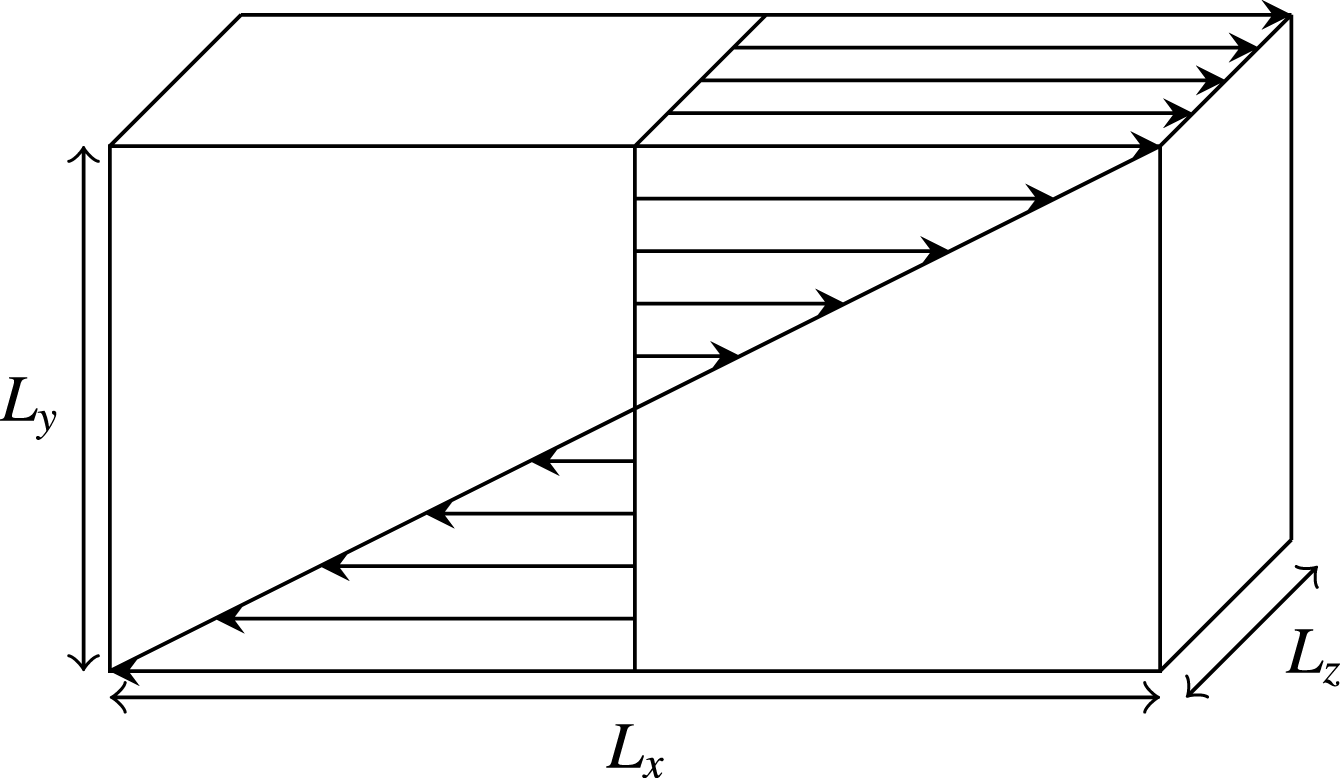
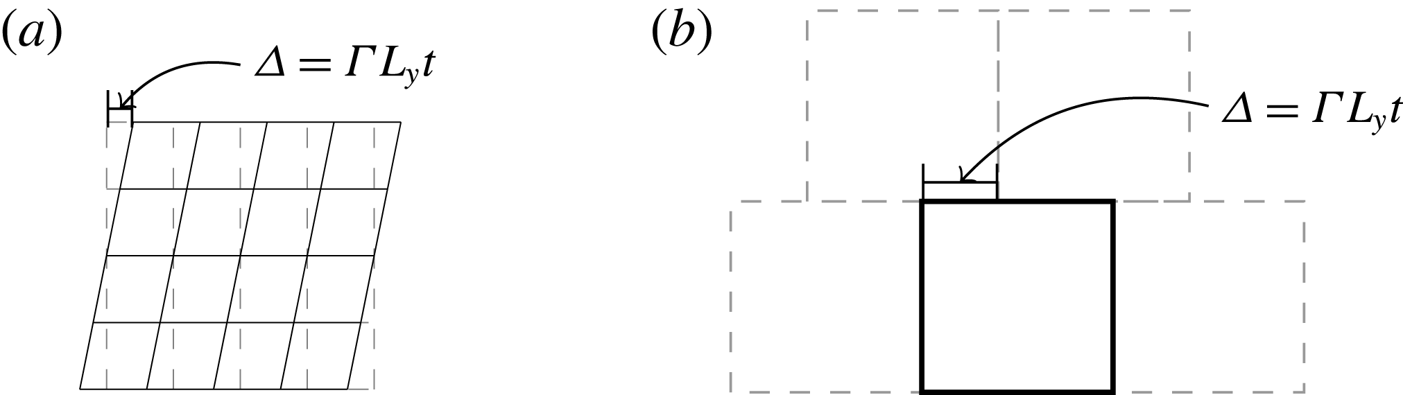
The simulation of HST (see figure 1 for a sketch of the geometry) and other homogeneously sheared cases requires the deployment of a special class of algorithms. The workhorse of most HST simulations is a pseudo-spectral algorithm developed by Rogallo (Reference Rogallo1981). In this approach, the governing equations are solved on a mesh that deforms with the mean flow (see figure 2 a). This method is widely popular due to the ease of implementation (Rogers & Moin Reference Rogers and Moin1987; Adrian & Moin Reference Adrian and Moin1988; Lee, Kim & Moin Reference Lee, Kim and Moin1990; Holt, Koseff & Ferziger Reference Holt, Koseff and Ferziger1992; Ishihara, Yoshida & Kaneda Reference Ishihara, Yoshida and Kaneda2002; Shotorban & Balachandar Reference Shotorban and Balachandar2006; Gualtieri et al. Reference Gualtieri, Casciola, Benzi and Piva2007a ; Jacobitz et al. Reference Jacobitz, Liechtenstein, Schneider and Farge2008, Reference Jacobitz, Schneider, Bos and Farge2010, Reference Jacobitz, Schneider, Bos and Farge2016; Chung & Matheou Reference Chung and Matheou2012; Salhi et al. Reference Salhi, Jacobitz, Schneider and Cambon2014). Challenges arising from different mean velocities at the two boundaries in the direction of the shear are circumvented by the use of simple periodic boundary conditions in the deforming mesh reference frame. Past a certain level of deformation, the solution is interpolated to a straightened mesh to restore the aspect ratio of the computational cells. The cost of remeshing can be severely penalizing and leads to discontinuous turbulence statistics. Brucker et al. (Reference Brucker, Isaza, Vaithianathan and Collins2007) estimated that up to 40 % of the turbulent kinetic energy can be lost over the long term, depending on the shear rate. They proposed another pseudo-spectral method which replaces the remeshing of the physical grid by a shift of wavenumber space at every iteration of the algorithm. The method achieves continuous statistics, but the long-time behaviour is plagued by Gibbs oscillations coming from the fine vortical structures in HST and requires the use of numerical dissipation for stabilization (Sukheswalla et al. Reference Sukheswalla, Vaithianathan and Collins2013).
The geometrical configuration. The velocity vectors illustrate the mean shear given by
 $(\unicode[STIX]{x1D6E4}y,0,0)$
.

In Rogallo’s method (a) the governing equations are solved on a deforming mesh allowing for normal periodicity in all directions. Baron’s method (b) solves the equations on a straight mesh using the shear-periodic boundary conditions to account for the displacement of the computational domain in the shear direction (Baron Reference Baron1982).

Another method was introduced by Baron (Reference Baron1982) and later improved by Schumann and coworkers (Schumann Reference Schumann and Boujot1985; Schumann, Elghobashi & Gerz Reference Schumann, Elghobashi, Gerz, Schumann and Friedrich1986; Gerz et al.
Reference Gerz, Schumann and Elghobashi1989). This method solves the equations in physical space without the need for remeshing as in Rogallo’s method. To do so, it relies on two key elements. First, the so-called shear-periodic boundary conditions are employed (see figure 2
b). For a quantity of interest
 $f$
, these boundary conditions apply in the following way:
 $$\begin{eqnarray}f(x,L_{y},z)=f(x-\unicode[STIX]{x1D6E4}tL_{y},0,z),\end{eqnarray}$$
where
 $\unicode[STIX]{x1D6E4}$
is the shear rate and
 $L_{y}$
is the domain size in the shear direction
 $y$
. Second, an operator splitting is used when solving the momentum equation, leaving the convection by mean shear for a separate step. The authors conducted a series of tests on stably stratified HST (Gerz et al.
Reference Gerz, Schumann and Elghobashi1989; Kaltenbach, Gerz & Schumann Reference Kaltenbach, Gerz and Schumann1994; Schumann Reference Schumann1996) and showed promising results. However, the complex interplay between the operator splitting, the boundary conditions and the interpolation method has not been fully unveiled. Additionally, it is stated in Schumann et al. (Reference Schumann, Elghobashi, Gerz, Schumann and Friedrich1986) that the method is unstable, and particularly so at higher resolutions, for longer simulation times and for unstratified HST, which is less numerically stable than the stratified situation.
To understand the issues with the method in Gerz et al. (Reference Gerz, Schumann and Elghobashi1989), we consider rotating waves, a class of solutions fundamental to homogeneously sheared flows. In addition to being relevant to a variety of problems (single phase flows (Thomson Reference Thomson1887), particle-laden flows (Kasbaoui et al.
Reference Kasbaoui, Koch, Subramanian and Desjardins2015), granular flows (Schmid & Kytomaa Reference Schmid and Kytomaa1994), accretion disks (Goldreich & Tremaine Reference Goldreich and Tremaine1978; Johnson & Gammie Reference Johnson and Gammie2005; Salhi et al.
Reference Salhi, Jacobitz, Schneider and Cambon2014), etc.), rotating waves have a direct application to HST. The rapid distortion theory (RDT) (Moffatt Reference Moffatt1965; Townsend Reference Townsend1970; Maxey Reference Maxey1982; Rogers Reference Rogers1991; Pope Reference Pope2001; Isaza & Collins Reference Isaza and Collins2009), applicable when the mean deformation greatly exceeds the nonlinear effects, shows that the fluctuating velocity
 $\boldsymbol{u}$
, defined as the deviation from the mean shear, can be expressed as a series of ‘rotating’ Fourier modes,
 $$\begin{eqnarray}\boldsymbol{u}(\boldsymbol{x},t)=\int \int \int \left\{\!\unicode[STIX]{x1D63C}(\boldsymbol{k}_{0},t)\hat{\boldsymbol{u}}_{0}\exp \!\left(\!-\unicode[STIX]{x1D708}t\!\left(\!k^{2}-k_{x,0}k_{y,0}\unicode[STIX]{x1D6E4}t+\frac{(k_{x,0}\unicode[STIX]{x1D6E4}t)^{2}}{3}\right)\!\right)\exp (\text{i}\boldsymbol{k}(t)\boldsymbol{\cdot }\boldsymbol{x})\!\right\}\,\text{d}\boldsymbol{k}_{0},\end{eqnarray}$$
where
 $\unicode[STIX]{x1D63C}$
is the RDT matrix (Maxey Reference Maxey1982; Isaza & Collins Reference Isaza and Collins2009), defined in appendix A, and
 $\hat{\boldsymbol{u}}_{0}$
is the amplitude of the mode
 $\boldsymbol{k}_{0}=(k_{x,0},k_{y,0},k_{z,0})$
at a chosen time origin. The evolution of the wavevector (and thus the orientation and wavelength of the mode) results from the shear,
 $\text{d}\boldsymbol{k}/\text{d}t=\unicode[STIX]{x1D6E4}\boldsymbol{e}_{y}\boldsymbol{e}_{x}\boldsymbol{\cdot }\boldsymbol{k}$
. We find that the method proposed by Gerz et al. (Reference Gerz, Schumann and Elghobashi1989) cannot maintain the normal structure of these waves. This deficiency is probably the reason for its lack of robustness. We resolve these issues with a careful execution of the operator splitting and timing of the shear-periodic boundary conditions.
The improved method combined with an energy-conserving discretization tailored for turbulence simulations (Desjardins et al.
Reference Desjardins, Blanquart, Balarac and Pitsch2008) allows us to produce statistics of HST for long times (
 $\unicode[STIX]{x1D6E4}t=20$
) without artificial stabilization. Direct numerical simulations of HST suffer from a loss of resolution at large times caused by the continuous production of finer turbulent structures by the shear straining. Simulations found in the literature run typically until
 $\unicode[STIX]{x1D6E4}t\sim 10$
(Lee et al.
Reference Lee, Kim and Moin1990; Brucker et al.
Reference Brucker, Isaza, Vaithianathan and Collins2007; Isaza & Collins Reference Isaza and Collins2009, Reference Isaza and Collins2011). The extension of the time window is critical to determining the nature of HST at long time.
With the ability to simulate for this long, we are in a position to compare our results with experiments and assess the sensitivity of the self-similar state to the initial conditions. The anisotropy of HST is also of interest and will be discussed.
This paper is organized as follows. Section 2 presents the governing equations. Section 3 goes into the details of the numerical approach. Rotating modes are used to understand the shortcomings of the method introduced in Gerz et al. (Reference Gerz, Schumann and Elghobashi1989). A fix is proposed and is verified to faithfully capture the rotating modes. In § 4, we use the algorithm to simulate HST. We present an extensive comparison with available experiments. A self-similar state, only weakly sensitive to the initial conditions, is found. Agreement with RDT is shown to hold until
 $\unicode[STIX]{x1D6E4}t\sim 5$
. We finally look into measures of local anisotropy in § 5.
2 Governing equations
The governing equations for an incompressible Newtonian fluid are
 $$\begin{eqnarray}\displaystyle & \displaystyle \frac{\unicode[STIX]{x2202}\boldsymbol{U}}{\unicode[STIX]{x2202}t}+\boldsymbol{U}\boldsymbol{\cdot }\unicode[STIX]{x1D735}\boldsymbol{U}=-\frac{1}{\unicode[STIX]{x1D70C}}\unicode[STIX]{x1D735}p+\unicode[STIX]{x1D708}\unicode[STIX]{x1D6FB}^{2}\boldsymbol{U}, & \displaystyle\end{eqnarray}$$
 $$\begin{eqnarray}\displaystyle & \displaystyle \unicode[STIX]{x1D735}\boldsymbol{\cdot }\boldsymbol{U}=0, & \displaystyle\end{eqnarray}$$
where
 $\boldsymbol{U}$
,
 $p$
,
 $\unicode[STIX]{x1D70C}$
and
 $\unicode[STIX]{x1D708}$
are the fluid velocity, pressure, density and kinematic viscosity respectively. The flow is subject to a mean shear wherein the flow is in the
 $x$
direction and varies in the
 $y$
direction with a shear rate
 $\unicode[STIX]{x1D6E4}$
(see figure 1) given by
 $(\unicode[STIX]{x1D6E4}y,0,0)$
. In the study of homogeneously sheared flow, a first step consists of separating the velocity fluctuations
 $\boldsymbol{u}$
from the mean shear motion
 $$\begin{eqnarray}\displaystyle \boldsymbol{U}=\unicode[STIX]{x1D6E4}y\boldsymbol{e}_{x}+\boldsymbol{u}. & & \displaystyle\end{eqnarray}$$
Introduction of the shear decomposition (2.3) in the governing equations (2.1) and (2.2) yields the evolution equations of the fluctuating part of the velocity field,
 $$\begin{eqnarray}\displaystyle & \displaystyle \frac{\unicode[STIX]{x2202}\boldsymbol{u}}{\unicode[STIX]{x2202}t}+\boldsymbol{u}\boldsymbol{\cdot }\unicode[STIX]{x1D735}\boldsymbol{u}=-\frac{1}{\unicode[STIX]{x1D70C}}\unicode[STIX]{x1D735}p+\unicode[STIX]{x1D708}\unicode[STIX]{x1D6FB}^{2}\boldsymbol{u}-\unicode[STIX]{x1D6E4}y\frac{\unicode[STIX]{x2202}\boldsymbol{u}}{\unicode[STIX]{x2202}x}-\unicode[STIX]{x1D6E4}u_{y}\boldsymbol{e}_{x}, & \displaystyle\end{eqnarray}$$
 $$\begin{eqnarray}\displaystyle & \displaystyle \unicode[STIX]{x1D735}\boldsymbol{\cdot }\boldsymbol{u}=0. & \displaystyle\end{eqnarray}$$
Two new terms appear in the momentum equation for the fluctuating velocity. The
 $\unicode[STIX]{x1D6E4}u_{y}\boldsymbol{e}_{x}$
term is a production of streamwise momentum caused by the convection of mean shear by the fluctuating velocity. The second term,
 $\unicode[STIX]{x1D6E4}y(\unicode[STIX]{x2202}\boldsymbol{u}/\unicode[STIX]{x2202}x)$
, arises due to the convection of fluctuations by the mean shear. As we explain below, it is this term that requires a careful implementation.
3 Numerical strategy
The approach discussed by Gerz et al. (Reference Gerz, Schumann and Elghobashi1989) solves (2.4) and (2.5) in physical space in the reference frame of the laboratory. These equations are completed by the shear-periodic boundary conditions (1.1) in the shear direction
 $y$
, and periodic boundary conditions in the other two directions. As recognized by Gerz et al. (Reference Gerz, Schumann and Elghobashi1989), special handling of the convection by the homogeneous shear term is required.
In a finite volume code, direct implementation of
 $\unicode[STIX]{x1D6E4}y(\unicode[STIX]{x2202}\boldsymbol{u}/\unicode[STIX]{x2202}x)$
as a source term is problematic. Errors associated with the discretization of the derivative are further magnified by the inhomogeneous coordinate
 $y$
multiplying the term. A severe consequence for HST simulations is the breaking of the homogeneity of the fluctuating velocity field. To circumvent this, Gerz et al. (Reference Gerz, Schumann and Elghobashi1989) proposed a solution that relies on operator splitting and spectral interpolations for the shear-periodic boundary conditions. The method was tested on stratified HST (Kaltenbach et al.
Reference Kaltenbach, Gerz and Schumann1994; Schumann Reference Schumann1996) and proved to be superior to the classic Rogallo algorithm (Rogallo Reference Rogallo1981). However, the method is recognized to be ‘weakly unstable’ (Schumann Reference Schumann and Boujot1985), and we will show that it fails to capture the analytical Kelvin modes.
To understand how these issues can be addressed, we start by summarizing the key ideas from Gerz et al. (Reference Gerz, Schumann and Elghobashi1989). The first step towards finding
 $\boldsymbol{u}^{n+1}$
consists of updating the velocity with an Adam–Bashforth scheme using the previous solutions
 $\boldsymbol{u}^{n}$
and
 $\boldsymbol{u}^{n-1}$
, i.e.
 $$\begin{eqnarray}\displaystyle \tilde{\boldsymbol{u}}=\boldsymbol{u}^{n}+\unicode[STIX]{x0394}t\left({\textstyle \frac{3}{2}}{\mathcal{M}}(\boldsymbol{u}^{n})-{\textstyle \frac{1}{2}}{\mathcal{M}}(\boldsymbol{u}^{n-1})\right), & & \displaystyle\end{eqnarray}$$
where
 ${\mathcal{M}}$
is the momentum operator from which the shear convection term is omitted,
 $$\begin{eqnarray}\displaystyle {\mathcal{M}}(\boldsymbol{u})=\unicode[STIX]{x1D708}\unicode[STIX]{x1D6FB}^{2}\boldsymbol{u}-\unicode[STIX]{x1D735}\boldsymbol{\cdot }(\boldsymbol{u}\boldsymbol{u})-\unicode[STIX]{x1D6E4}u_{y}\boldsymbol{e}_{x}. & & \displaystyle\end{eqnarray}$$
Next, the convection by shear is included using
 $$\begin{eqnarray}\check{\boldsymbol{u}}(\boldsymbol{x})=\tilde{\boldsymbol{u}}(\boldsymbol{x}-\unicode[STIX]{x0394}t\unicode[STIX]{x1D6E4}y\boldsymbol{e}_{x}).\end{eqnarray}$$
This is equivalent to solving the equation of pure convection by homogeneous shear,
 $$\begin{eqnarray}\frac{\unicode[STIX]{x2202}\boldsymbol{u}}{\unicode[STIX]{x2202}t}+\unicode[STIX]{x1D6E4}y\boldsymbol{e}_{x}\boldsymbol{\cdot }\frac{\unicode[STIX]{x2202}\boldsymbol{u}}{\unicode[STIX]{x2202}x}=0,\end{eqnarray}$$
using the method of characteristics over a time interval
 $\unicode[STIX]{x0394}t$
. We term step (3.3) the ‘shear-remapping’ operation because it maps local values to upstream ones. The boundary conditions (1.1) are then applied at time
 $n+1$
. Finally, the pressure-Poisson equation is solved and the velocity is updated,
 $$\begin{eqnarray}\displaystyle & \displaystyle \unicode[STIX]{x1D6FB}^{2}p^{n+1}=\frac{1}{\unicode[STIX]{x0394}t}\unicode[STIX]{x1D735}\boldsymbol{\cdot }\check{\boldsymbol{u}}, & \displaystyle\end{eqnarray}$$
 $$\begin{eqnarray}\displaystyle & \displaystyle \boldsymbol{u}^{n+1}=\check{\boldsymbol{u}}-\frac{\unicode[STIX]{x0394}t}{\unicode[STIX]{x1D70C}}\unicode[STIX]{x1D735}p^{n+1}. & \displaystyle\end{eqnarray}$$
This is efficiently done with a spectral preconditioner in the
 $x$
and
 $z$
directions. A linear system is solved for the direction
 $y$
with a careful implementation of the boundary conditions. Further details can be found in Schumann (Reference Schumann and Boujot1985).
In most cases in the literature, validation of codes dealing with homogeneously sheared flows has been conducted on HST with the goal of obtaining statistics that are in accordance with experiments or turbulence theories (Pope Reference Pope2001). In such complex flows, it is easy to miss numerical errors. A stronger test case is a comparison against the analytical Kelvin modes. These are the individual modes appearing in the RDT expansion (1.2). In 2D (
 $k_{z}=0$
), a Kelvin mode reads
 $$\begin{eqnarray}\displaystyle & \displaystyle u_{y}^{K}(\boldsymbol{x},t)=\left(\frac{k_{0}}{k}\right)^{2}\exp \left(-\unicode[STIX]{x1D708}t\left(k^{2}-k_{x}k_{y,0}\unicode[STIX]{x1D6E4}t+\frac{(k_{x}\unicode[STIX]{x1D6E4}t)^{2}}{3}\right)\right)u_{y,0}\exp (\text{i}\boldsymbol{k}\boldsymbol{\cdot }\boldsymbol{x}), & \displaystyle\end{eqnarray}$$
 $$\begin{eqnarray}\displaystyle & \displaystyle u_{x}^{K}(\boldsymbol{x},t)=-\frac{k_{y}(t)}{k_{x}}u_{y}^{K}(\boldsymbol{x},t), & \displaystyle\end{eqnarray}$$
 $$\begin{eqnarray}\displaystyle & \displaystyle k_{y}=k_{y,0}-k_{x}\unicode[STIX]{x1D6E4}t. & \displaystyle\end{eqnarray}$$
In the above,
 $\boldsymbol{k}(t)=(k_{x},k_{y})$
is the rotating wavevector of the Kelvin mode, the magnitude of which is
 $k=\sqrt{k_{x}^{2}+k_{y}^{2}}$
(i.e. the wavenumber). According to (3.9), the orientation of the wave changes over time to align with the shear direction
 $\boldsymbol{e}_{y}$
. The wavelength increases when the wavevector is in the stretching quadrant of the homogeneous shear (
 $k_{x}k_{y}>0$
) and decreases in the compressive quadrant (
 $k_{x}k_{y}<0$
). The Kelvin mode is a solution to the full Navier–Stokes equations and decays in a superexponential fashion. These attributes make it an excellent way of validating numerical codes. A desirable feature of any algorithm is the ability to keep the level of numerical errors below the magnitude of the mode, even as it decays. The simulation of Kelvin modes has the potential to quickly expose numerical artefacts due to the very fast decay of the solution.
We performed simulations with the method above on a 2D square domain. The algorithm was implemented in the CFD code NGA (Desjardins et al.
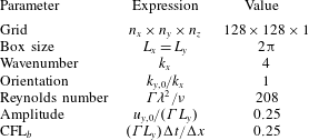
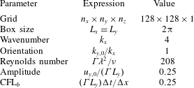
Reference Desjardins, Blanquart, Balarac and Pitsch2008), on a staggered mesh and with a second-order discretization. The simulation parameters are listed in table 1. The initial wavevector was
 $45^{\circ }$
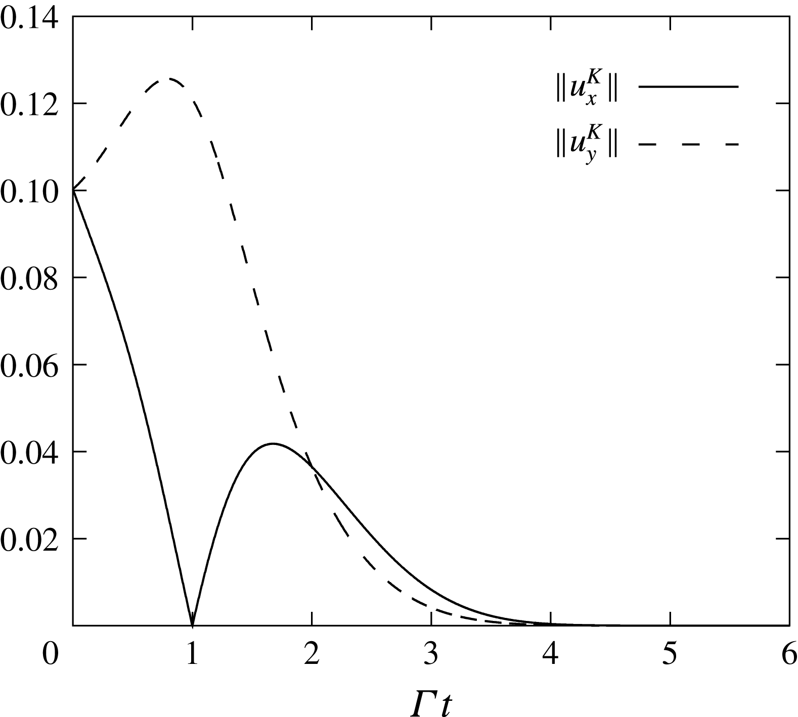
upstream of the gradient direction with four periods in the domain. Figure 3 reports the time evolution of the velocity amplitudes of the Kelvin mode based on the analytical expressions (3.7)–(3.9). It should be noticed that these quantities decay exponentially, and that at
 $\unicode[STIX]{x1D6E4}t=1$
,
 $\hat{u} _{x}^{K}$
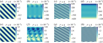
vanishes because the wavevector becomes horizontal. Snapshots of the simulation with the method of Gerz et al. (Reference Gerz, Schumann and Elghobashi1989) are given in figure 4(a–d) for non-dimensional time
 $\unicode[STIX]{x1D6E4}t$
going from 0 to 5. The figure shows isocontours of the horizontal component of velocity
 $u_{x}$
. While we do observe rotation of the wave, the horizontal velocity does not vanish to machine precision at
 $\unicode[STIX]{x1D6E4}t=1$
. Furthermore, numerical errors eventually dominate the solution, with errors being largest near the top and bottom boundaries,
 $y=\pm L_{y}/2$
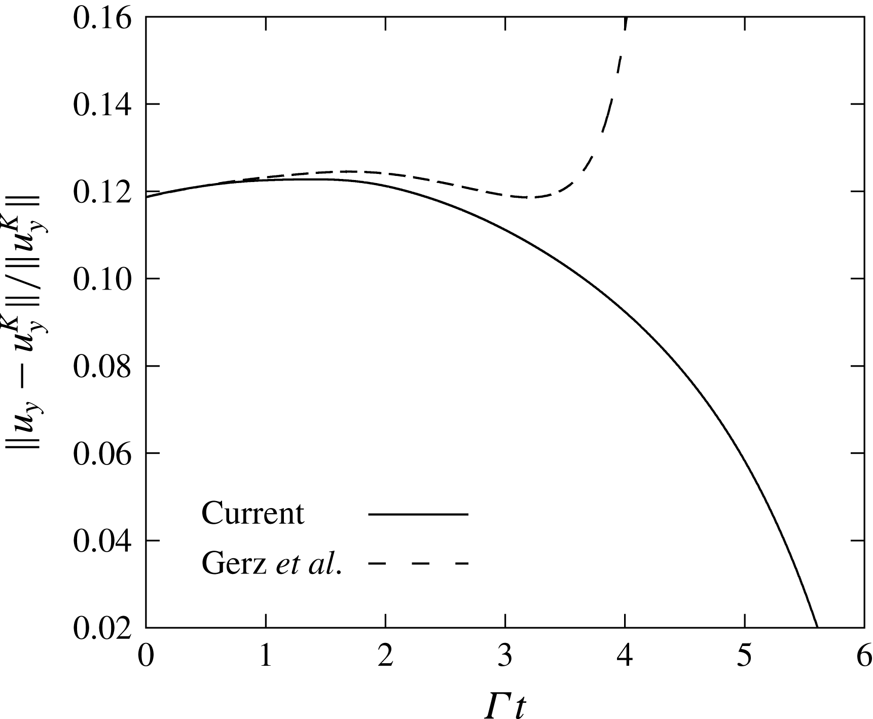
. A look at the relative error of the
 $y$
component in figure 7 also shows that errors dominate the solution after
 $\unicode[STIX]{x1D6E4}t\sim 4$
.
The magnitude of the theoretical Kelvin mode with the parameters from table 1.

Parameters for simulating the Kelvin modes given in non-dimensional form. The Reynolds number is defined using the perturbation wavelength
 $\unicode[STIX]{x1D706}=\sqrt{(2\unicode[STIX]{x03C0}/k_{x})^{2}+(2\unicode[STIX]{x03C0}/k_{y,0})^{2}}$
and base shear flow seen by the perturbation (
 $\unicode[STIX]{x1D6E4}\unicode[STIX]{x1D706}$
). The base Courant–Friedrichs–Lewy number
 $\text{CFL}_{b}$
is associated with the base shear flow in the simulation domain (
 $\unicode[STIX]{x1D6E4}L_{y}$
).
Snapshots of a Kelvin mode perturbation at the non-dimensional times
 $t^{\star }=\unicode[STIX]{x1D6E4}t=0$
, 1, 4 and 5 using the approach of Gerz et al. (Reference Gerz, Schumann and Elghobashi1989) (a–d) and the new method (e–h). The new algorithm maintains the normal structure of the wave perturbation as it is turned and dissipated at all times. The original method described by Gerz et al. (Reference Gerz, Schumann and Elghobashi1989) does not preserve the structure of a wave. The errors are most visible when the horizontal perturbation vanishes at
 $\unicode[STIX]{x1D6E4}t=1$
and when the wave is quickly dissipated by viscosity (
 $\unicode[STIX]{x1D6E4}t>4$
).

The problem with the algorithm of Gerz et al. (Reference Gerz, Schumann and Elghobashi1989) is the incompatibility between the time discretization and the operator splitting. These two need to work hand in hand because the shear-periodic boundary conditions are time-dependent. In particular, the Adam–Bashforth time integrator is ill-advised here because it convolves waves with different orientations (
 $\boldsymbol{u}^{n}$
and
 $\boldsymbol{u}^{n-1}$
).
To understand why this is an issue, let us consider the simpler equation parametrized by a constant
 $A>0$
,
 $$\begin{eqnarray}\frac{\unicode[STIX]{x2202}u}{\unicode[STIX]{x2202}t}+\unicode[STIX]{x1D6E4}y\frac{\unicode[STIX]{x2202}u}{\unicode[STIX]{x2202}x}=Au.\end{eqnarray}$$
Despite being radically simpler than the Navier–Stokes equation and unbounded, this equation still captures some of the physics of homogeneously sheared flows. In fact, the turbulent kinetic energy in the self-similar regime of HST (discussed in the following section) displays exponential growth that obeys (3.10) above. Solutions of the form of turning waves,
 $u=\hat{u} (t)\exp (\text{i}\boldsymbol{k}\boldsymbol{\cdot }\boldsymbol{x})$
, must satisfy
 $$\begin{eqnarray}\displaystyle & \displaystyle \frac{\text{d}\boldsymbol{k}}{\text{d}t}\boldsymbol{\cdot }\boldsymbol{x}=-\unicode[STIX]{x1D6E4}y\boldsymbol{k}\boldsymbol{\cdot }\boldsymbol{e}_{x}, & \displaystyle\end{eqnarray}$$
 $$\begin{eqnarray}\displaystyle & \displaystyle \frac{\text{d}\hat{u} }{\text{d}t}=A\hat{u} . & \displaystyle\end{eqnarray}$$
Hence, we find that
 $u=u(0)\exp (At)\exp (\text{i}(k_{x}x+(k_{y,0}-k_{x}\unicode[STIX]{x1D6E4}t)y))$
is a solution to (3.10). The numerical solution is well behaved when any perturbations are of the same form, i.e. rotating waves that do not break the normal structure of the wave. In this case, the perturbations grow slowly and are not amplified in a relative sense. The discretization error
 $\unicode[STIX]{x1D716}$
, that is the difference between the numerical and analytical solutions, evolves according to the same equation (3.10). Now, suppose that these errors at the time steps
 $n$
and
 $n-1$
are waves of amplitudes
 $\hat{\unicode[STIX]{x1D716}}^{n}$
and
 $\hat{\unicode[STIX]{x1D716}}^{n-1}$
and wavevectors
 $\boldsymbol{k}^{n}$
and
 $\boldsymbol{k}^{n-1}$
. For clarity, the error at the
 $n$
th time step reads
 $$\begin{eqnarray}\unicode[STIX]{x1D716}^{n}=\hat{\unicode[STIX]{x1D716}}^{n}\exp (\text{i}\boldsymbol{k}^{n}\boldsymbol{\cdot }\boldsymbol{x}).\end{eqnarray}$$
At the next time step, the new error needs to retain the form (3.13) with a new wavevector and amplitude,
 $\boldsymbol{k}^{n+1}$
,
 $\hat{\unicode[STIX]{x1D716}}^{n+1}$
, that are discrete solutions to the ordinary differential equations (3.11) and (3.12).
With the algorithm above, the Adam–Bashforth integration yields an intermediary error
 $$\begin{eqnarray}\displaystyle \bar{\unicode[STIX]{x1D716}}^{n+1} & = & \displaystyle \unicode[STIX]{x1D716}^{n}+\unicode[STIX]{x0394}tA\left({\textstyle \frac{3}{2}}\hat{\unicode[STIX]{x1D716}}^{n}\exp (\text{i}\boldsymbol{k}^{n}\boldsymbol{\cdot }\boldsymbol{x})-{\textstyle \frac{1}{2}}\hat{\unicode[STIX]{x1D716}}^{n-1}\exp (\text{i}\boldsymbol{k}^{n-1}\boldsymbol{\cdot }\boldsymbol{x})\right)\end{eqnarray}$$
 $$\begin{eqnarray}\displaystyle & = & \displaystyle \left(\hat{\unicode[STIX]{x1D716}}^{n}+\unicode[STIX]{x0394}tA\left({\textstyle \frac{3}{2}}\hat{\unicode[STIX]{x1D716}}^{n}-{\textstyle \frac{1}{2}}\hat{\unicode[STIX]{x1D716}}^{n-1}\exp (-\text{i}\unicode[STIX]{x0394}\boldsymbol{k}\boldsymbol{\cdot }\boldsymbol{x})\right)\right)\exp (\text{i}\boldsymbol{k}^{n}\boldsymbol{\cdot }\boldsymbol{x}),\end{eqnarray}$$
where
 $\unicode[STIX]{x0394}\boldsymbol{k}=\boldsymbol{k}^{n}-\boldsymbol{k}^{n-1}$
. The application of the ‘shear-remapping’ step yields the error at
 $n+1$
,
 $$\begin{eqnarray}\displaystyle \unicode[STIX]{x1D716}^{n+1} & = & \displaystyle \overbrace{\left(\hat{\unicode[STIX]{x1D716}}^{n}+\unicode[STIX]{x0394}tA\left({\textstyle \frac{3}{2}}\hat{\unicode[STIX]{x1D716}}^{n}-~{\textstyle \frac{1}{2}}\hat{\unicode[STIX]{x1D716}}^{n-1}\exp \left(-\text{i}\unicode[STIX]{x0394}\boldsymbol{k}\boldsymbol{\cdot }(\boldsymbol{x}-\unicode[STIX]{x0394}t\unicode[STIX]{x1D6E4}y\boldsymbol{e}_{x})\right)\right)\right)}^{\hat{\unicode[STIX]{x1D716}}^{n+1}}\nonumber\\ \displaystyle & & \displaystyle \times \,\exp \underbrace{(\text{i}\boldsymbol{k}^{n}\boldsymbol{\cdot }(\boldsymbol{x}-\unicode[STIX]{x0394}t\unicode[STIX]{x1D6E4}y\boldsymbol{e}_{x}))}_{\text{i}\boldsymbol{k}^{n+1}\boldsymbol{\cdot }\boldsymbol{x}}.\end{eqnarray}$$
Let us examine whether this update preserves the structure of a wave. First, the phase of the update (3.16) can be recast with a new wavevector
 $\boldsymbol{k}^{n+1}$
in the following way:
 $$\begin{eqnarray}\boldsymbol{k}^{n}\boldsymbol{\cdot }(\boldsymbol{x}-\unicode[STIX]{x0394}t\unicode[STIX]{x1D6E4}y\boldsymbol{e}_{x})=\boldsymbol{k}^{n+1}\boldsymbol{\cdot }\boldsymbol{x}.\end{eqnarray}$$
Further reorganization of the result above shows that the new wavevector is indeed a solution to (3.11),
 $$\begin{eqnarray}\frac{\boldsymbol{k}^{n+1}-\boldsymbol{k}^{n}}{\unicode[STIX]{x0394}t}\boldsymbol{\cdot }\boldsymbol{x}=-\unicode[STIX]{x1D6E4}y\boldsymbol{k}^{n}\boldsymbol{\cdot }\boldsymbol{e}_{x}.\end{eqnarray}$$
This is actually an exact solution of (3.11) because the wavevector is a linear function of time.
The amplitude
 $\hat{\unicode[STIX]{x1D716}}^{n+1}$
in the update (3.16) is, however, not a valid one and does not satisfy the condition (3.12). The failure is caused by the presence of spatial coordinates in its expression, and precisely because of the different orientations (
 $\unicode[STIX]{x0394}\boldsymbol{k}\neq 0$
) of the right-hand side between
 $n-1$
and
 $n$
. The problematic term can be simplified as follows:
 $$\begin{eqnarray}\exp (-\text{i}\unicode[STIX]{x0394}\boldsymbol{k}\boldsymbol{\cdot }(\boldsymbol{r}-\unicode[STIX]{x0394}t\unicode[STIX]{x1D6E4}y\boldsymbol{e}_{x}))=\exp (-\text{i}k_{x}\unicode[STIX]{x1D6E4}y\unicode[STIX]{x0394}t)\sim 1-\text{i}k_{x}\unicode[STIX]{x1D6E4}y\unicode[STIX]{x0394}t,\end{eqnarray}$$
showing that the errors will be larger at the top and bottom of the domain. This is consistent with previous observations.
In addition to distorting the wave, numerical errors grow faster than the analytical solution. The error amplitude can be cast in the form
 $\hat{\unicode[STIX]{x1D716}}^{n}=\text{e}^{\unicode[STIX]{x1D6FC}(y)n\unicode[STIX]{x0394}t}$
, similarly to the analytical amplitude but with a growth rate that depends on
 $y$
. From (3.16), the relative amplification
 $R=\text{e}^{\unicode[STIX]{x1D6FC}(y)\unicode[STIX]{x0394}t}$
between steps
 $n$
and
 $n-1$
satisfies
 $$\begin{eqnarray}R^{2}(y)-\left(1+\frac{3}{2}A\unicode[STIX]{x0394}t\right)R(y)+\frac{A\unicode[STIX]{x0394}tC(y)}{2}=0,\end{eqnarray}$$
where
 $C(y)=\exp (\text{i}k_{x}\unicode[STIX]{x1D6E4}y\unicode[STIX]{x0394}t)$
. Because we expect the scheme to fare the worst at the top and bottom boundaries, let us work directly at
 $y=L_{y}/2$
and consider the highest wavenumber,
 $k_{x}=\unicode[STIX]{x03C0}n_{x}/L_{x}$
. We see that for these parameters,
 $C=\exp (\text{i}\unicode[STIX]{x03C0}\text{CFL}_{b}/2)$
, where
 $\text{CFL}_{b}=\unicode[STIX]{x1D6E4}L_{y}\unicode[STIX]{x0394}t/\unicode[STIX]{x0394}x$
is the convective Courant–Friedrichs–Lewy number for the base shear. With a reasonable time step
 $A\unicode[STIX]{x0394}t=0.1$
and
 $\text{CFL}_{b}=0.9$
, we find that
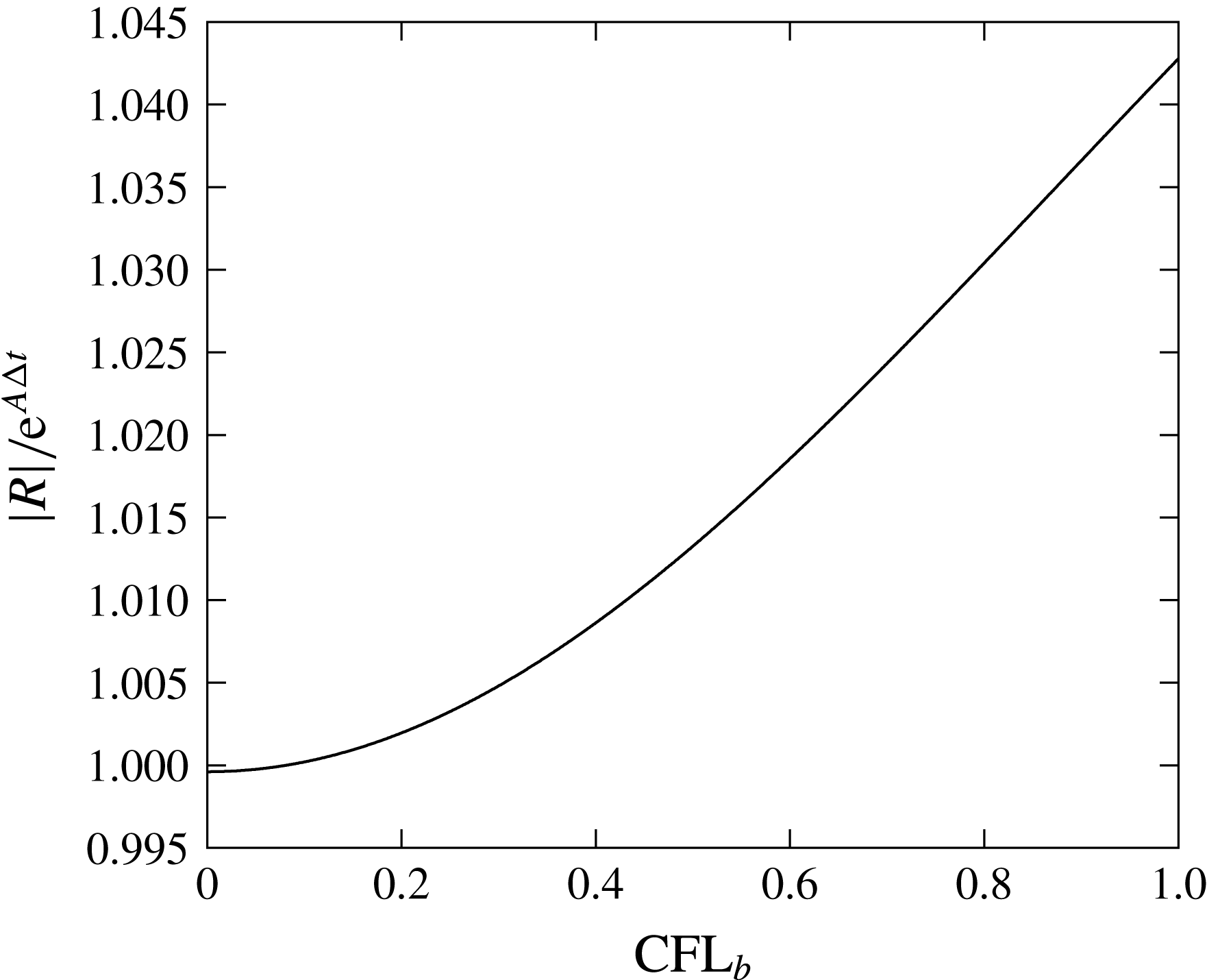
 $\left|R\right|/\text{e}^{A\unicode[STIX]{x0394}t}\sim 1.036$
. This indicates that distortions and cell to cell numerical instabilities are likely to occur near the boundaries of the domain. Figure 5 shows that the relative amplification of the error becomes lower than that of the analytical solutions only for prohibitively small
 $\text{CFL}_{b}$
numbers.
We now propose an approach that builds on the method of Gerz et al. (Reference Gerz, Schumann and Elghobashi1989) to ensure stability, robustness and adequate simulation of rotating waves.
The ratio of the error amplification between
 $n$
and
 $n+1$
to the amplification of the analytical solution. The value is given for the highest wavenumber admissible in the simulation grid,
 $k_{x}=\unicode[STIX]{x03C0}n_{x}/L_{x}$
, and at position
 $y=L_{y}/2$
. Cell to cell numerical oscillations are expected for a ratio larger than one.

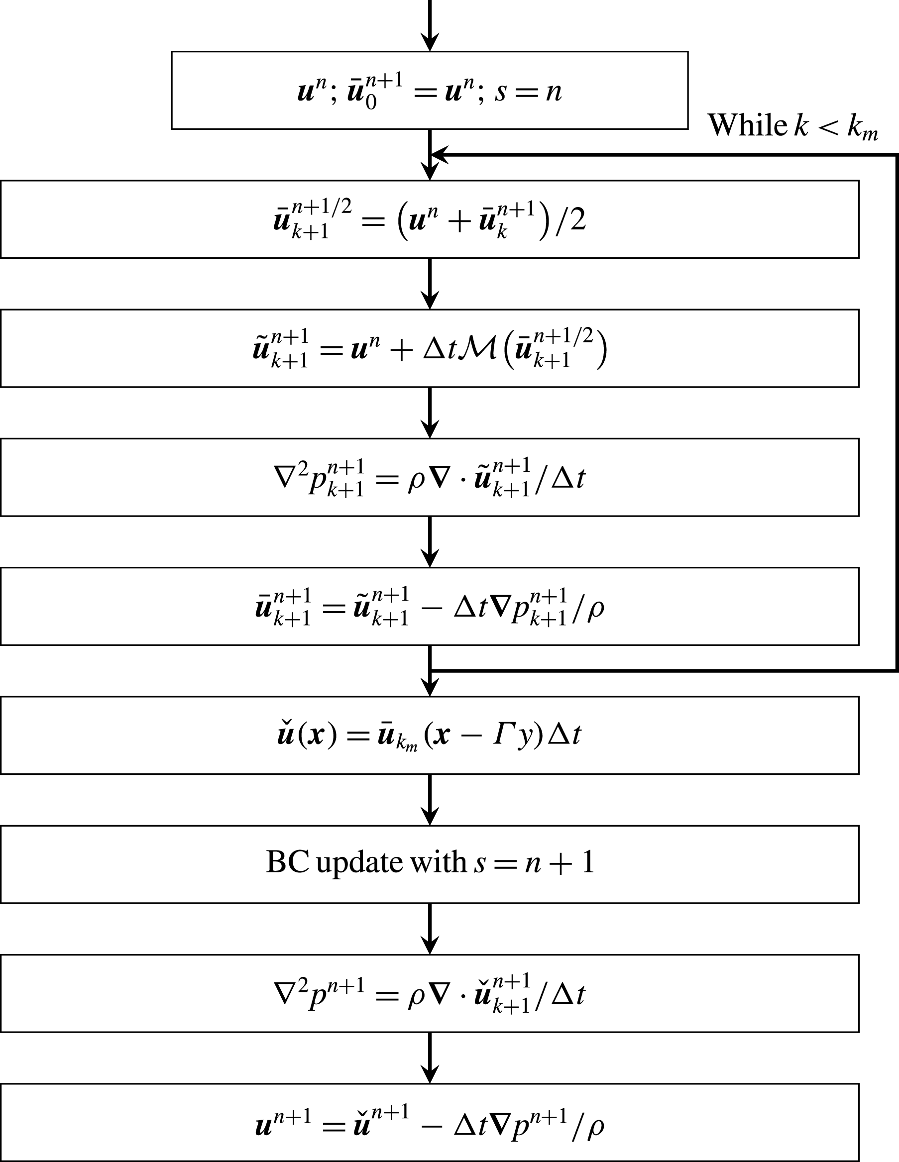
Figure 6 presents an overview of the algorithm. Coming from the realization that we cannot use solutions from previous time steps, we replace the Adam–Bashforth time integration with an explicit scheme that builds the solution at
 $n+1$
using states at
 $n$
only. In the following, we employ the iterative Crank–Nicolson method (Pierce Reference Pierce2001). Solution of the Crank–Nicolson scheme by iterations turns it into an explicit scheme that satisfies the condition of building
 $n+1$
quantities from quantities at the time step
 $n$
only. The use of two iterations per time step leads to a second-order-accurate scheme. A larger number of iterations leads to stability properties approaching those of the fully implicit scheme in the sense of Von Neumann analyses (Teukolsky Reference Teukolsky2000; Pierce Reference Pierce2001).
Summary of the algorithm with the operator splitting and shear-periodic boundary conditions.

Let us focus on the
 $(k+1)$
th sub-iteration. To find the update
 $\bar{\boldsymbol{u}}_{k+1}^{n+1}$
at the end of sub-iteration
 $k+1$
, we start by estimating the quantities at mid-step, i.e.
 $$\begin{eqnarray}\bar{\boldsymbol{u}}_{k+1}^{n+1/2}=\frac{\boldsymbol{u}^{n}+\bar{\boldsymbol{u}}_{k}^{n+1}}{2}.\end{eqnarray}$$
We will also keep track of a counter
 $s$
, corresponding to the time at which the boundary conditions are applied. At the start of the sub-iteration, we have
 $s=n$
. Next, we solve the momentum equation without the convection by the shear term,
 $$\begin{eqnarray}\tilde{\boldsymbol{u}}_{k+1}^{n+1}=\boldsymbol{u}^{n}+\unicode[STIX]{x0394}t{\mathcal{M}}(\bar{\boldsymbol{u}}_{k+1}^{n+1/2}).\end{eqnarray}$$
The pressure-Poisson equation is then solved, and the solenoidal condition is enforced,
 $$\begin{eqnarray}\displaystyle \unicode[STIX]{x1D6FB}^{2}p_{k+1}^{n+1}=\unicode[STIX]{x1D70C}\frac{\unicode[STIX]{x1D735}\boldsymbol{\cdot }\tilde{\boldsymbol{u}}_{k+1}^{n+1}}{\unicode[STIX]{x0394}t}, & & \displaystyle\end{eqnarray}$$
 $$\begin{eqnarray}\displaystyle \bar{\boldsymbol{u}}_{k+1}^{n+1}=\tilde{\boldsymbol{u}}_{k+1}^{n+1}-\frac{\unicode[STIX]{x0394}t}{\unicode[STIX]{x1D70C}}\unicode[STIX]{x1D735}p_{k+1}^{n+1}. & & \displaystyle\end{eqnarray}$$
It should be noticed that the necessary boundary conditions updated before the pressure-Poisson step are still applied with the time of step
 $n$
. At this point, we loop through these steps for a maximum number of sub-iterations
 $k_{m}$
. The next steps consist of applying the shear-remapping, updating the shear timer
 $s$
, solving a new pressure-Poisson system and reinforcing the solenoidal condition,
 $$\begin{eqnarray}\displaystyle & \displaystyle \check{\boldsymbol{u}}^{n+1}(\boldsymbol{x})=\bar{\boldsymbol{u}}_{k_{m}}^{n+1}(\boldsymbol{x}-\unicode[STIX]{x1D6E4}y\unicode[STIX]{x0394}t), & \displaystyle\end{eqnarray}$$
 $$\begin{eqnarray}\displaystyle & \displaystyle s=n+1, & \displaystyle\end{eqnarray}$$
 $$\begin{eqnarray}\displaystyle & \displaystyle \unicode[STIX]{x1D6FB}^{2}p^{n+1}=\frac{\unicode[STIX]{x1D735}\boldsymbol{\cdot }\check{\boldsymbol{u}}^{n+1}}{\unicode[STIX]{x0394}t}, & \displaystyle\end{eqnarray}$$
 $$\begin{eqnarray}\displaystyle & \displaystyle \boldsymbol{u}^{n+1}=\check{\boldsymbol{u}}^{n+1}-\frac{\unicode[STIX]{x0394}t}{\unicode[STIX]{x1D70C}}\unicode[STIX]{x1D735}p^{n+1}. & \displaystyle\end{eqnarray}$$
It is important that the shear counter is updated right after the shear-remapping step and that all subsequent boundary conditions are applied with the new time. Additional information on the pressure solver can be found in Schumann (Reference Schumann and Boujot1985). The velocity field evaluations required for the shear-remapping step and the shear-periodic boundary conditions are obtained using discrete Fourier interpolations (Schumann et al. Reference Schumann, Elghobashi, Gerz, Schumann and Friedrich1986).
The operator splitting proposed in (Gerz et al.
Reference Gerz, Schumann and Elghobashi1989) and adopted here carries a splitting penalty that is first order in time. This is similar in principle to the widely accepted pressure correction approach for incompressible flows (referring to the decoupling of steps (3.22)–(3.24)), which is in essence a first-order operator splitting (Chorin Reference Chorin1968; Temam Reference Temam1968). Later studies (Dukowicz & Dvinsky Reference Dukowicz and Dvinsky1992; Akselvoll Reference Akselvoll1995; Wall, Pierce & Moin Reference Wall, Pierce and Moin2002) show that nesting of the advection-correction steps within the iterative Crank–Nicolson loop achieves formal second-order accuracy with
 $k_{m}=2$
sub-iterations. In practice, two or three sub-iterations are used with this algorithm (Teukolsky Reference Teukolsky2000; Pierce Reference Pierce2001).
Various extensions to the explicit Iterative Crank–Nicolson scheme exist, although generally at increasing computational cost. Akselvoll (Reference Akselvoll1995) and Pierce (Reference Pierce2001) computed and inverted an incomplete Jacobian of the Navier–Stokes equations within the algorithm loop in order to treat parts of the viscous dissipation and convection implicitly. A fully implicit Crank–Nicolson scheme has also been derived and applied by Choi, Moin & Kim (Reference Choi, Moin and Kim1993) and Choi & Moin (Reference Choi and Moin1994). In DNS of turbulence where all scales are amply resolved, the explicit iterative Crank–Nicolson is a satisfactory scheme that is computationally cheaper than implicit implementations, robust and second-order accurate. Further details on the numerical properties of this family of schemes can be found in Kim & Moin (Reference Kim and Moin1985), Orszag, Israeli & Deville (Reference Orszag, Israeli and Deville1986) and Gresho (Reference Gresho1990).
To improve the time accuracy associated with the additional shear-remapping step, it would be tempting to perform this inside the Crank–Nicolson loop. However, the present analysis aims to show that this is not as trivial as it may seem. As we have shown with the Von Neumann analysis of the errors above, the interpolation (3.21) would lead to a mid-step velocity
 $\bar{\boldsymbol{u}}_{k+1}^{n+1/2}$
that does not preserve the normality of the rotating waves, because
 $\bar{\boldsymbol{u}}_{k}^{n+1}$
would be ‘shear-remapped’ one more time than
 $\boldsymbol{u}^{n}$
. This causes the solver to be numerically unstable. For robustness, it is crucial to leave the shear-remapping outside of the Crank–Nicolson loop.
Other time integration procedures can be used to replace the Crank–Nicolson as long as all time interpolations are based on states with the same degree of ‘shear-remapping’. For instance, a Von Neumann analysis of (3.10) would show that a second-order Runge–Kutta integration scheme could be employed without breaking the normal structure of the rotating waves. Unlike the Adam–Bashforth scheme, which mixes states at
 $n$
and
 $n-1$
, the Runge–Kutta scheme uses a mid-step state that is a linear combination of states at
 $n$
only. We rely on the iterative Crank–Nicolson for the reasons explained above.
For the test problem (3.10), this algorithm yields an error at
 $n+1$
of the form
 $$\begin{eqnarray}\displaystyle \unicode[STIX]{x1D716}^{n+1}=\hat{\unicode[STIX]{x1D716}}^{n}\left(\mathop{\sum }_{k=0}^{k_{m}}\frac{(\unicode[STIX]{x0394}tA)^{k}}{k!}\right)\exp (\text{i}\boldsymbol{k}^{n+1}\boldsymbol{\cdot }\boldsymbol{r}). & & \displaystyle\end{eqnarray}$$
Because the amplitude of the error at
 $n+1$
is independent of the inhomogeneous coordinate
 $y$
, the structure of the wave is preserved. Additionally, the rate of growth of errors,
 $R=\unicode[STIX]{x1D716}^{n+1}/\unicode[STIX]{x1D716}^{n}$
, is strictly smaller than the rate of growth of the analytical solution
 $\text{e}^{A\unicode[STIX]{x0394}t}$
. When tested on the Kelvin modes, the relative errors, shown in figure 7, are significantly lower than previously found with the method of Gerz et al. (Reference Gerz, Schumann and Elghobashi1989). Snapshots of the horizontal velocity isocontours, figure 4(e–h), show that the structure of the rotating wave remains intact even as it rotates and dissipates.
In contrast to the methods of Rogallo (Reference Rogallo1981) and Gerz et al. (Reference Gerz, Schumann and Elghobashi1989), there is no
 $\text{CFL}_{b}$
restriction with this approach. This property derives from the characteristic method employed in the shear-remapping step. Combined with NGA’s arbitrarily high-order spatial discretization on a staggered mesh (Desjardins et al.
Reference Desjardins, Blanquart, Balarac and Pitsch2008), the implementation conserves mass, momentum and kinetic energy in a discrete sense. We primarily use a second-order discretization for the simulation of HST, although fourth- and sixth-order discretizations are also considered.
The relative error from the simulations of Kelvin modes using the approach of Gerz et al. (Reference Gerz, Schumann and Elghobashi1989) and the one presented here. When the perturbation starts to dissipate (
 $\unicode[STIX]{x1D6E4}t>3$
), numerical errors quickly dominate in the original approach of Gerz et al. (Reference Gerz, Schumann and Elghobashi1989).

4 Direct numerical simulation of homogeneously sheared turbulence
In this section, we seek to further validate the numerical approach and explore the physics of homogeneous shear turbulence. An analysis of the long-time statistics is undertaken to test the universality of the self-similar regime. We provide comparisons with experimental data and predictions from rapid distortion theory (RDT). To understand whether the flow achieves local isotropy, we consider the statistics of the transverse velocity derivative.
The flow is initialized with the turbulence spectrum provided in Isaza & Collins (Reference Isaza and Collins2009) (IC),
 $$\begin{eqnarray}\displaystyle E_{0}(k)=C_{k}\unicode[STIX]{x1D716}_{0}^{2/3}\unicode[STIX]{x1D705}_{0}^{-5/3}\left\{\begin{array}{@{}ll@{}}(k/\unicode[STIX]{x1D705}_{0})^{2}, & k<\unicode[STIX]{x1D705}_{0},\\ (k/\unicode[STIX]{x1D705}_{0})^{-5/3}, & \unicode[STIX]{x1D705}_{0}\leqslant k\leqslant \unicode[STIX]{x1D705}_{\unicode[STIX]{x1D702}},\\ 0, & k>\unicode[STIX]{x1D705}_{\unicode[STIX]{x1D702}},\end{array}\right. & & \displaystyle\end{eqnarray}$$
where
 $\unicode[STIX]{x1D716}_{0}$
is the initial dissipation rate,
 $\unicode[STIX]{x1D705}_{0}$
is the spectrum peak wavenumber and
 $C_{k}=1.5$
is a constant. The largest wavenumber,
 $\unicode[STIX]{x1D705}_{\unicode[STIX]{x1D702}}$
, follows:
 $$\begin{eqnarray}\unicode[STIX]{x1D705}_{\unicode[STIX]{x1D702}}=\unicode[STIX]{x1D705}_{0}\left[\frac{2\unicode[STIX]{x1D716}_{0}^{1/3}}{3\unicode[STIX]{x1D708}C_{k}\unicode[STIX]{x1D705}_{0}^{4/3}}+\frac{11}{15}\right]^{3/4}.\end{eqnarray}$$
This flow is characterized by two non-dimensional numbers, the Taylor-microscale Reynolds number
 $Re_{\unicode[STIX]{x1D706}}=\unicode[STIX]{x1D706}(q^{2}/3)^{1/2}/\unicode[STIX]{x1D708}$
, based on the microscale
 $\unicode[STIX]{x1D706}=\sqrt{15\unicode[STIX]{x1D708}q^{2}/(3\unicode[STIX]{x1D716})}$
, and the shear number
 $S^{\ast }=\unicode[STIX]{x1D6E4}q^{2}/\unicode[STIX]{x1D716}$
, where
 $q^{2}$
is twice the kinetic energy. In HST,
 $Re_{\unicode[STIX]{x1D706}}$
and
 $S^{\ast }$
are dynamic quantities varying with increasing total strain
 $\unicode[STIX]{x1D6E4}t$
. We denote the initial values with a subscript 0. It should be noted that alternative definitions of
 $Re_{\unicode[STIX]{x1D706}}$
can be found in the literature. For instance, a number of experimental studies report results in terms of the longitudinal Taylor-microscale
 $\unicode[STIX]{x1D706}_{xx}=\sqrt{\langle u_{x}^{2}\rangle /\langle (\unicode[STIX]{x2202}u_{x}/\unicode[STIX]{x2202}x)^{2}\rangle }$
and the corresponding Reynolds number
 $Re_{\unicode[STIX]{x1D706}_{xx}}=\langle u_{x}^{2}\rangle ^{1/2}\unicode[STIX]{x1D706}_{xx}/\unicode[STIX]{x1D708}$
. The brackets in these expressions denote spatial averaging. The two Taylor microscales can be found from one another using
 $\unicode[STIX]{x1D716}=5\unicode[STIX]{x1D708}q^{2}/\unicode[STIX]{x1D706}^{2}=15\unicode[STIX]{x1D708}\langle u_{x}^{2}\rangle /\unicode[STIX]{x1D706}_{xx}^{2}$
, which requires knowledge of the second moment of the velocity. When only two velocity components are measured, we estimate
 $q^{2}=(1+\unicode[STIX]{x1D6FC})(\langle u_{x}^{2}\rangle +\langle u_{y}^{2}\rangle )$
. The quantity
 $\unicode[STIX]{x1D6FC}=\langle u_{z}^{2}\rangle /(\langle u_{x}^{2}\rangle +\langle u_{y}^{2}\rangle )$
is estimated at 0.43 by Isaza et al. (Reference Isaza, Warhaft and Collins2009), in agreement with prior experimental measurements.
There has been much debate in the literature about whether this flow reaches a self-similar state. According to George & Gibson (Reference George and Gibson1992) and Pope (Reference Pope2001), this is a state attained once the flow is controlled by a single time scale. This regime is observed when the following features apply.
-
(i) The kinetic energy
 $q^{2}$
grows exponentially, taking the form
$q^{2}/q_{0}^{2}\propto \exp (\unicode[STIX]{x1D70E}\unicode[STIX]{x1D6E4}t)$
, where
$\unicode[STIX]{x1D70E}$
is the growth rate.
-
(ii) Statistics normalized by the shear rate
$\unicode[STIX]{x1D6E4}$
and kinetic energy become independent of time. These include the ratio of the production rate
${\mathcal{P}}=-\unicode[STIX]{x1D6E4}\langle u_{x}u_{y}\rangle$
to the dissipation rate
$\unicode[STIX]{x1D716}$
, the shear number
$S^{\ast }$
and the anisotropic Reynolds stress tensor
$\unicode[STIX]{x1D623}_{ij}=\langle u_{i}u_{j}\rangle /q^{2}-\unicode[STIX]{x1D6FF}_{ij}/3$
. -
(iii) The integral length scale
$L_{11}=\int _{0}^{\infty }u_{x}(x,y,z)u_{x}(x+r,y,z)\text{d}r/\langle u_{x}^{2}\rangle$
, when scaled by
$q/\unicode[STIX]{x1D6E4}$
, reaches a constant.







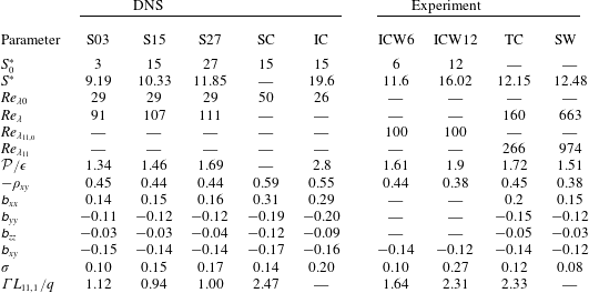
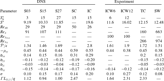
Virtually all experiments indicate the existence of a self-similar state. Experiments by Tavoularis & Corrsin (Reference Tavoularis and Corrsin1981) (TC), Rohr et al. (Reference Rohr, Itsweire, Helland and Atta1988), Tavoularis & Karnik (Reference Tavoularis and Karnik1989) (TK), Shen & Warhaft (Reference Shen and Warhaft2000) (SW) and Isaza et al. (Reference Isaza, Warhaft and Collins2009) (ICW) find asymptotic states consistent with the requirement of self-similarity. On the other hand, DNS studies offer a more uncertain view of the long-time state. The simulations of Lee et al. (Reference Lee, Kim and Moin1990) (based on Rogallo’s method) do not achieve a self-similar state, whereas the DNS of Isaza & Collins (Reference Isaza and Collins2009) (IC) and Sukheswalla et al. (Reference Sukheswalla, Vaithianathan and Collins2013) (SC) (both based on the pseudo-spectral method of Brucker et al. (Reference Brucker, Isaza, Vaithianathan and Collins2007)) indicate the opposite. Table 2 reports a compilation of data from the literature.
Comparisons of the present asymptotic DNS statistics (S03, S15, S27) with previous DNS and experiments: SC, Sukheswalla et al. (Reference Sukheswalla, Vaithianathan and Collins2013); IC, Isaza & Collins (Reference Isaza and Collins2009); ICW, Isaza et al. (Reference Isaza, Warhaft and Collins2009); TC, Tavoularis & Corrsin (Reference Tavoularis and Corrsin1981); SW, Shen & Warhaft (Reference Shen and Warhaft2000). When the kinetic energy is not reported in experiments, it is estimated preferably with
 $q^{2}=1.43(\langle u_{x}^{2}\rangle +\langle u_{y}^{2}\rangle )$
or with
 $q^{2}=2\langle u_{x}^{2}\rangle$
.
In the self-similar regime, the dependence of the asymptotic values on the initial conditions is still an open question. In the case of a self-similar regime independent of
 $S_{0}^{\ast }$
and
 $Re_{\unicode[STIX]{x1D706},0}$
, the long-time values of
 ${\mathcal{P}}/\unicode[STIX]{x1D716}$
,
 $S^{\ast }$
and
 $\unicode[STIX]{x1D623}_{ij}$
would be universal quantities. Experimental evidence for the universality of the long-time state with different initial conditions is not clear cut. SW and TC found comparable asymptotic values (see table 2), despite the different facilities, Reynolds numbers and shear rates considered. In both cases, the asymptotic shear number
 $S^{\ast }$
and the ratio
 ${\mathcal{P}}/\unicode[STIX]{x1D716}$
were found to be close to 12 and 1.6 respectively. This was further confirmed by ICW in their lower-initial-shear-number experiment (ICW6). Nonetheless, the latter group found a higher pair
 $(S^{\ast },{\mathcal{P}}/\unicode[STIX]{x1D716})$
in their larger-initial-shear-number experiment (ICW12). They also reported that the variation of
 $Re_{\unicode[STIX]{x1D706},0}$
leads to no change in the asymptotic values. The conclusion we draw from these experiments is that the asymptotic state is likely to be independent of
 $Re_{\unicode[STIX]{x1D706},0}$
, but the dependence on
 $S_{0}^{\ast }$
is unresolved. As we explain later, we find from our simulations little sensitivity to the initial shear number in the self-similar regime.
In this study, we performed three runs termed S03, S15 and S27, corresponding to the initial shear numbers
 $S_{0}^{\ast }=3$
, 15 and 27 respectively, and initial Reynolds number
 $Re_{\unicode[STIX]{x1D706}0}=29$
for all three cases. The choice of three distinct shear numbers allows analysis of the sensitivity of the long-time state to this quantity. In addition, cases S15 and S27 have sufficiently high shear numbers to allow for comparisons with RDT.
The parameters for the three runs considered in this study.

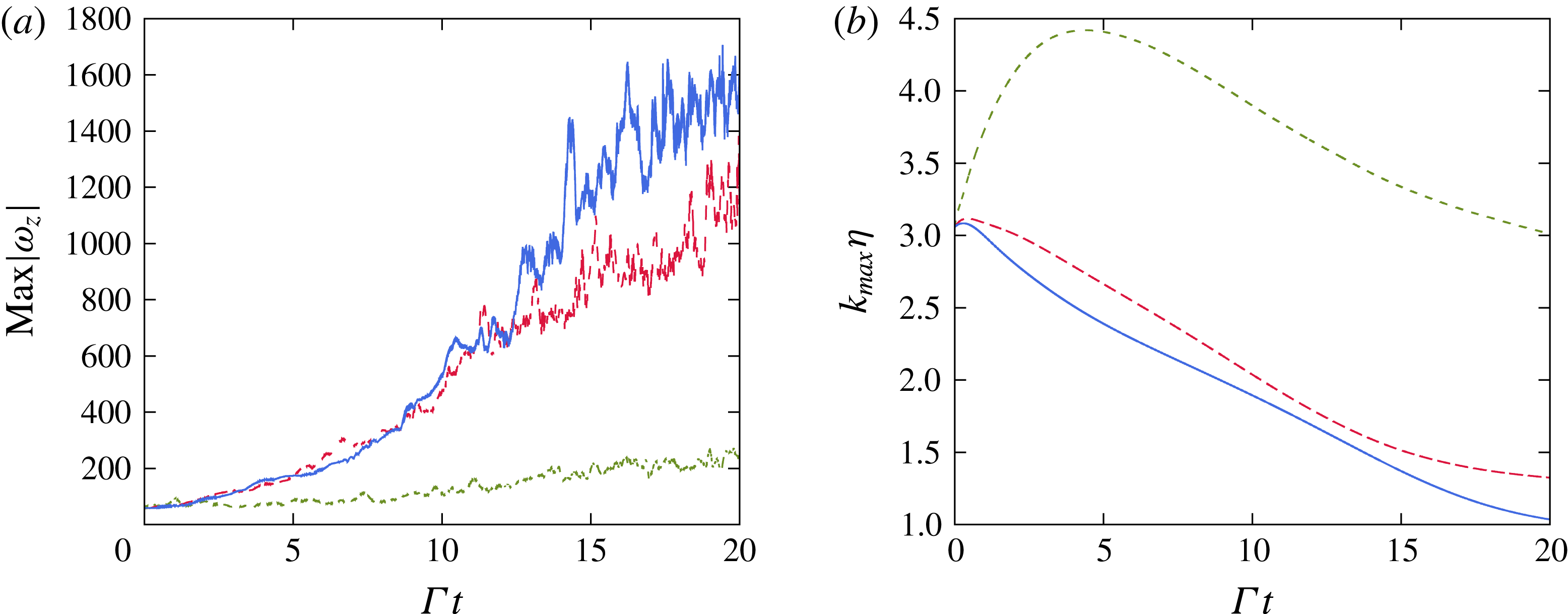
The evolution of the maximum vorticity in the
 $z$
direction (a) and the product of the largest resolved wavenumber with the Kolmogorov length scale (b) for the three cases considered: ——, S27; – –, S15;
 $\cdots \,$
, S03. The bounded evolution of the vorticity shows the stability of the numerics. The small scales of the turbulence are well resolved when
 $k_{max}\unicode[STIX]{x1D702}>1$
.

Details of the simulation set-up are given in table 3. The choice of parameters follows the DNS of SC and is based on a thorough discussion in IC. It is argued that the correct resolution of all scales is of paramount importance to achieving a self-similar state. The challenge in HST is that the large scales grow and the small scales decrease as the simulation progresses. For a given mesh, a loss of resolution is inevitable. The integration time window can be extended by the choice of a finer grid at greater computational cost. We performed our simulations with 2 billion grid cells and limited the integration to the dimensionless time
 $\unicode[STIX]{x1D6E4}t=20$
. Figure 8(b) shows that adequate resolution of the small scales is achieved for all cases by maintaining
 $k_{max}\unicode[STIX]{x1D702}\geqslant 1$
, where
 $k_{max}$
is the largest resolved wavenumber and
 $\unicode[STIX]{x1D702}=(\unicode[STIX]{x1D708}^{3}/\unicode[STIX]{x1D716})^{1/4}$
is the Kolmogorov length. It should be noted that the nearly monotonic decrease of
 $\unicode[STIX]{x1D702}$
is in agreement with the experimental findings of Tavoularis & Corrsin (Reference Tavoularis and Corrsin1981) as well as Rohr et al. (Reference Rohr, Itsweire, Helland and Atta1988). The computational box remains amply larger than the largest turbulence scales. The integral length scale
 $L_{11}$
, a measure of these scales, remains
 ${<}0.07L_{x}$
at all times for the three simulations.
We note that a subset of the literature considered integration times significantly longer than
 $\unicode[STIX]{x1D6E4}t=20$
but at significantly lower resolutions. Pumir & Shraiman (Reference Pumir and Shraiman1995) employed Rogallo’s method, which is stable to very long times but with a loss of kinetic energy due to remeshing (Brucker et al.
Reference Brucker, Isaza, Vaithianathan and Collins2007), to run simulations until
 $\unicode[STIX]{x1D6E4}t=210$
at a resolution of
 $144^{3}$
. More recently, Gualtieri et al. (Reference Gualtieri, Casciola, Benzi and Piva2007a
) ran simulations until
 $\unicode[STIX]{x1D6E4}t=870$
at a resolution of
 $256\times 256\times 128$
. Other similar approaches include those of Pumir (Reference Pumir1996), Schumacher & Eckhardt (Reference Schumacher and Eckhardt2000), Schumacher (Reference Schumacher2001), Gualtieri et al. (Reference Gualtieri, Casciola, Benzi, Amati and Piva2002) and Schumacher (Reference Schumacher2004). These simulations are, by design, confined by the numerical box. The goal of these studies is generally to achieve statistical stationarity where the production rate balances the dissipation rate, and the small scales are bounded by the mesh resolution. While confinement by the box may have its own purposes (see Gualtieri et al.
Reference Gualtieri, Casciola, Benzi and Piva2007a
), these settings do not allow the manifestation of the self-similar regime, a state of significant imbalance between production and dissipation and continuously decreasing small scales.
4.1 Numerical robustness
Before considering the physics of these flows, we address the numerical feasibility of the simulations. Figure 8(a) reports the maximum vorticity in the
 $z$
direction for all three runs. The signal is noisy (as for any instantaneous quantity in a turbulent field) but remains bounded nevertheless. In the simulations of SC, this quantity diverges around
 $\unicode[STIX]{x1D6E4}t\sim 10$
and is believed to be the root of the instability of the simulations. The remedy proposed consisted of damping the small-scale features with a spectral filter every few time steps. This fix stabilizes the method of Brucker et al. (Reference Brucker, Isaza, Vaithianathan and Collins2007) at the expense of making it more dissipative. Detailed study of the effects of the filter in SC shows that the dissipation rate is strongly affected by the filtration procedure and cannot be faithfully captured by this approach (Sukheswalla et al.
Reference Sukheswalla, Vaithianathan and Collins2013). Our attempts to run these cases with the original method of Gerz et al. (Reference Gerz, Schumann and Elghobashi1989) also failed quite rapidly (around
 $\unicode[STIX]{x1D6E4}t\sim 2$
). We ran these cases using the numerical method described in § 3 without the input of any artificial viscosity or dissipation processes, retaining the most accurate numerical properties.
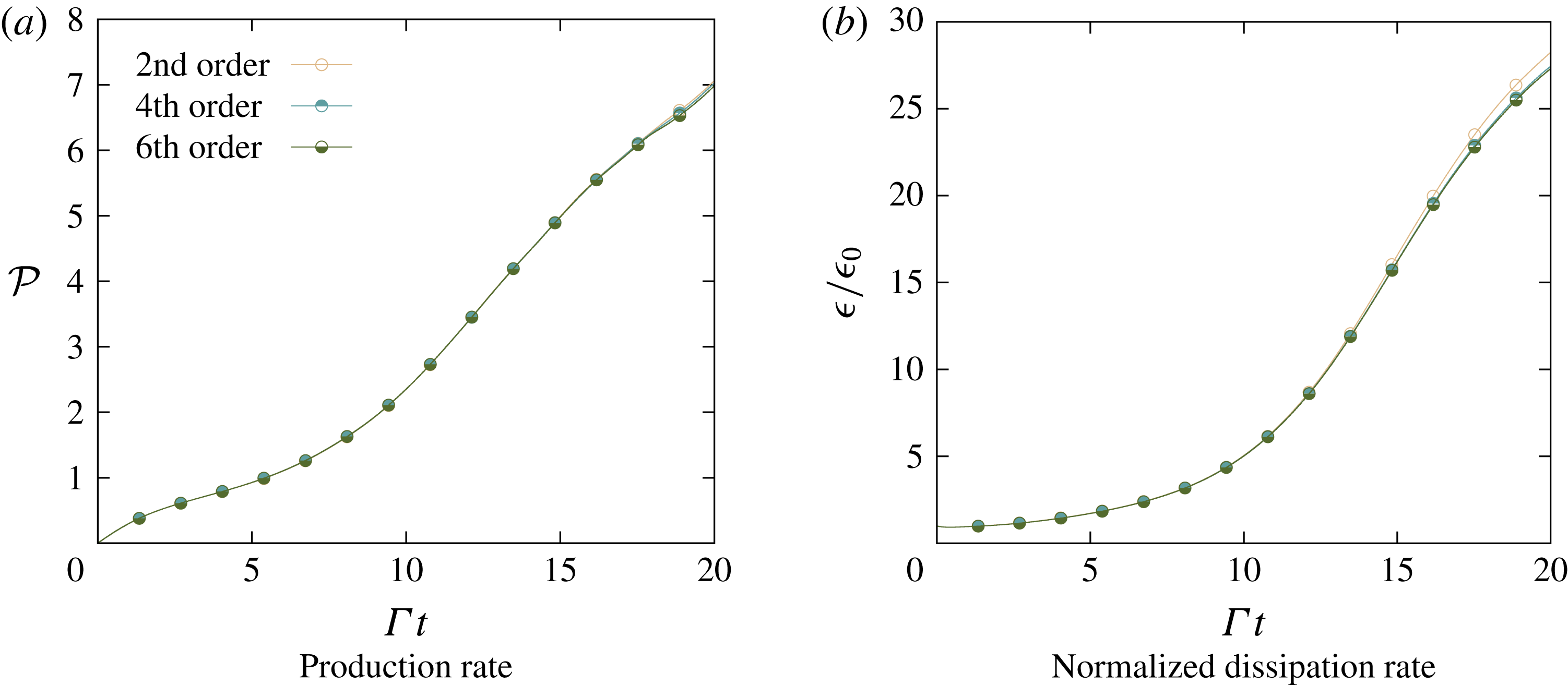
To test the effect of the spatial discretization, we ran case S15 with second-, fourth- and sixth-order discretizations. The production and dissipation rates are shown in figure 9. The discretization order affects primarily the small scales through the dissipation rate. Differences are manifested towards the end of the simulation,
 $\unicode[STIX]{x1D6E4}t\sim 20$
, but are very small given the ample resolution. We conclude that the second-order scheme is sufficient.
The effect of the spatial discretization on the large- (production rate) and small-scale (dissipation rate) statistics.

4.2 Analysis of the self-similar regime
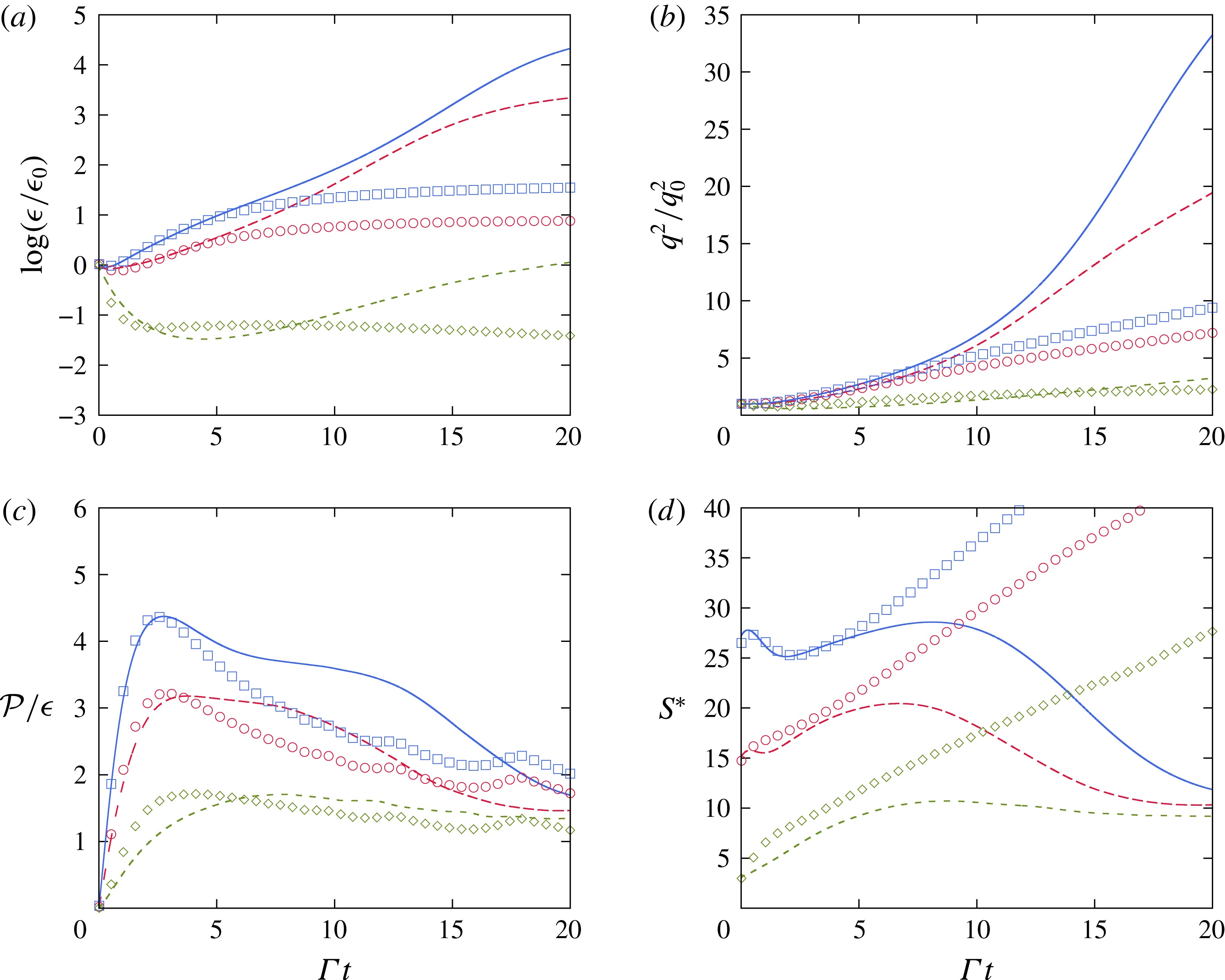
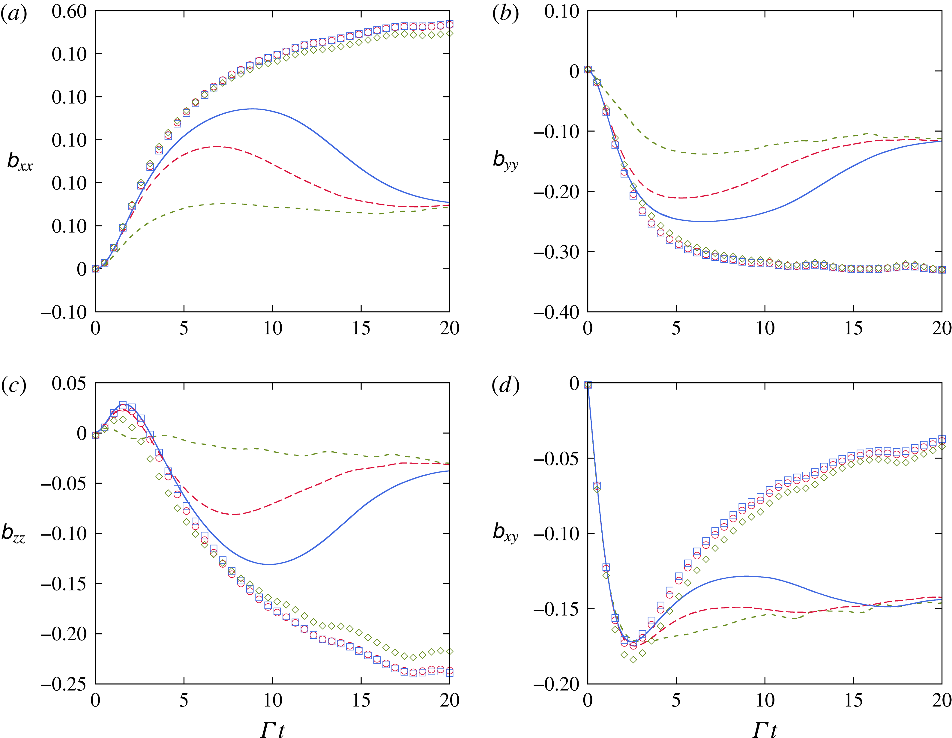
Some turbulence statistics: normalized dissipation rate (a), normalized kinetic energy (b), ratio of production rate to dissipation rate (c) and shear number (d). The DNS (lines) show a self-similar regime weakly sensitive to the initial shear number: ——, S27; – –, S15;
 $\cdots \,$
, S03. The viscous RDT (symbols) shows agreement for total strains
 $\unicode[STIX]{x1D6E4}t\leqslant 5$
: ▫, S27; ○, S15; ♢, S03.

The temporal evolutions of the normalized dissipation rate
 $\unicode[STIX]{x1D716}/\unicode[STIX]{x1D716}_{0}$
, normalized kinetic energy
 $q^{2}/q_{0}^{2}$
, ratio of production to dissipation rates
 ${\mathcal{P}}/\unicode[STIX]{x1D716}$
and shear number
 $S^{\ast }$
are presented in figure 10. Both the dissipation rate and the kinetic energy are seen to grow exponentially after
 $\unicode[STIX]{x1D6E4}t\sim 5$
. This is consistent with previous DNS and experiments as well as the requirement for a self-similar state. The growth rate
 $\unicode[STIX]{x1D70E}$
of the kinetic energy depends on the initial shear number
 $S_{0}^{\ast }$
. A fit to the DNS data for times
 $4\leqslant \unicode[STIX]{x1D6E4}t\leqslant 20$
yields
 $\unicode[STIX]{x1D70E}=0.10$
for the medium-shearing case S03 and
 $\unicode[STIX]{x1D70E}=0.15$
and 0.17 for the high-shearing cases S15 and S27 respectively. These values are close to the ones reported by SC (0.12, 0.14 and 0.13 for their simulations with initial shear numbers of 3, 15 and 27 respectively and
 $Re_{\unicode[STIX]{x1D706}0}=50$
). However, unlike SC, we observe a monotonic increase in
 $\unicode[STIX]{x1D70E}$
with increasing shear number. One might expect a monotonic increase in
 $\unicode[STIX]{x1D70E}$
with increasing
 $S_{0}^{\ast }$
based on previous observations in the experimental and theoretical literature. It is known from Tavoularis (Reference Tavoularis1985) that the growth rate is a function of the shear number and initial length scale of the flow. The theoretical analysis in George & Gibson (Reference George and Gibson1992) of the self-similar state points towards a growth rate that increases with increasing shear rate
 $\unicode[STIX]{x1D6E4}$
for similar initial turbulence spectra. Furthermore, the experiments of Isaza et al. (Reference Isaza, Warhaft and Collins2009) (ICW6 and ICW12) hint towards positive correlations between these two quantities (see table 2). Definitive conclusions would require the study of more than just two shear numbers. Experiments from TK report the growth rate for a large number of experiments but the shear number is varied at the same time as other parameters. It can be noted that a fit over the time window
 $4\leqslant \unicode[STIX]{x1D6E4}t\leqslant 9$
, as done in IC, yields values substantially close to those found in that study:
 $\unicode[STIX]{x1D70E}=0.12,~0.20,~0.20$
from our runs S03/S15/S27 and
 $\unicode[STIX]{x1D70E}=0.10,~0.20,~0.18$
from theirs. This seems to indicate that the total integration time in IC was not sufficiently long to attain a self-similar state. The experiments of TC and SW do not report the growth rate
 $\unicode[STIX]{x1D70E}$
. However, indirect comparisons can be made by considering the turbulent kinetic energy balance under the assumption of exponential growth (Tavoularis Reference Tavoularis1985),
 $$\begin{eqnarray}\displaystyle \unicode[STIX]{x1D70E}=\frac{1}{\unicode[STIX]{x1D6E4}q^{2}}\frac{\text{d}q^{2}}{\text{d}t} & = & \displaystyle 2\unicode[STIX]{x1D623}_{xy}\left(\frac{\unicode[STIX]{x1D716}}{{\mathcal{P}}}-1\right).\end{eqnarray}$$
Using this approach, we find
 $\unicode[STIX]{x1D70E}=0.12$
and
 $\unicode[STIX]{x1D70E}=0.08$
for the experiments of TC and SW respectively. These values are in approximate agreement with our findings.
At long times, the ratio of production to dissipation (figure 10
c) and the shear number (figure 10
d) tend to collapse to
 $S_{0}^{\ast }$
-independent asymptotic values for all three cases that are close to the ones reported by SW, TC and ICW. At the end of the simulations
 $\unicode[STIX]{x1D6E4}t=20$
,
 ${\mathcal{P}}/\unicode[STIX]{x1D716}=1.34$
, 1.51 and 1.63 and
 $S^{\ast }=9.18$
, 10.47 and 11.44 for S03, S15 and S27 respectively. For comparison, in their respective experiments, SW measured (
 ${\mathcal{P}}/\unicode[STIX]{x1D716},S^{\ast }$
)
 $=(1.51,12.22)$
, TC (
 ${\mathcal{P}}/\unicode[STIX]{x1D716},S^{\ast }$
)
 $=(1.72,12.15)$
and ICW (
 ${\mathcal{P}}/\unicode[STIX]{x1D716},S^{\ast }$
)
 $=(1.61,11.6)$
in their lower-initial-shear-number case. The latter group reported different plateaus in their high-
 $S_{0}^{\ast }$
experiment, but it is worth mentioning that this experiment relied on an active shear generator unlike the passive one used in their lower-
 $S_{0}^{\ast }$
experiment and by SW and TC. The constancy of
 ${\mathcal{P}}/\unicode[STIX]{x1D716}$
and
 $S^{\ast }$
in our simulations further corroborates the self-similarity of the flow. It is interesting to note that the asymptotic values seem to collapse despite the widely different initial shear numbers. Previous DNS found different trends. While Rogers (Reference Rogers1986) found asymptotic states insensitive to the initial conditions, the DNS of Rogallo (Reference Rogallo1981), Lee et al. (Reference Lee, Kim and Moin1990), Isaza & Collins (Reference Isaza and Collins2009) and Sukheswalla et al. (Reference Sukheswalla, Vaithianathan and Collins2013) indicated the opposite behaviour.
The anisotropic Reynolds stresses seen in figure 11 reach asymptotes independent of the initial shear number. These values are in good agreement with the experiments of TC and SW. The early evolutions of
 $\unicode[STIX]{x1D623}_{xx}$
,
 $\unicode[STIX]{x1D623}_{yy}$
,
 $\unicode[STIX]{x1D623}_{zz}$
and
 $\unicode[STIX]{x1D623}_{xy}$
also show very little sensitivity to the shear number. In the experiments of Isaza et al. (Reference Isaza, Warhaft and Collins2009), doubling the shear number led to no appreciable variation of
 $\unicode[STIX]{x1D623}_{xy}$
, which was found to be equal to
 $-0.12$
. It is possible that the asymptotic values might be controlled solely by the initial Reynolds number
 $Re_{\unicode[STIX]{x1D706}0}$
. The cross-correlation
 $\unicode[STIX]{x1D70C}_{xy}=\langle u_{x}u_{y}\rangle /\sqrt{\langle u_{x}^{2}\rangle \langle u_{y}^{2}\rangle }$
from our simulations reaches a value of
 $-0.45$
, in agreement with most experiments. In contrast, most DNS studies, including the ones shown in table 2, find values in the range
 $-0.5$
to
 $-0.6$
(Sukheswalla et al.
Reference Sukheswalla, Vaithianathan and Collins2013).
Anisotropic stress tensor components. The lines and symbols are as in figure 10.

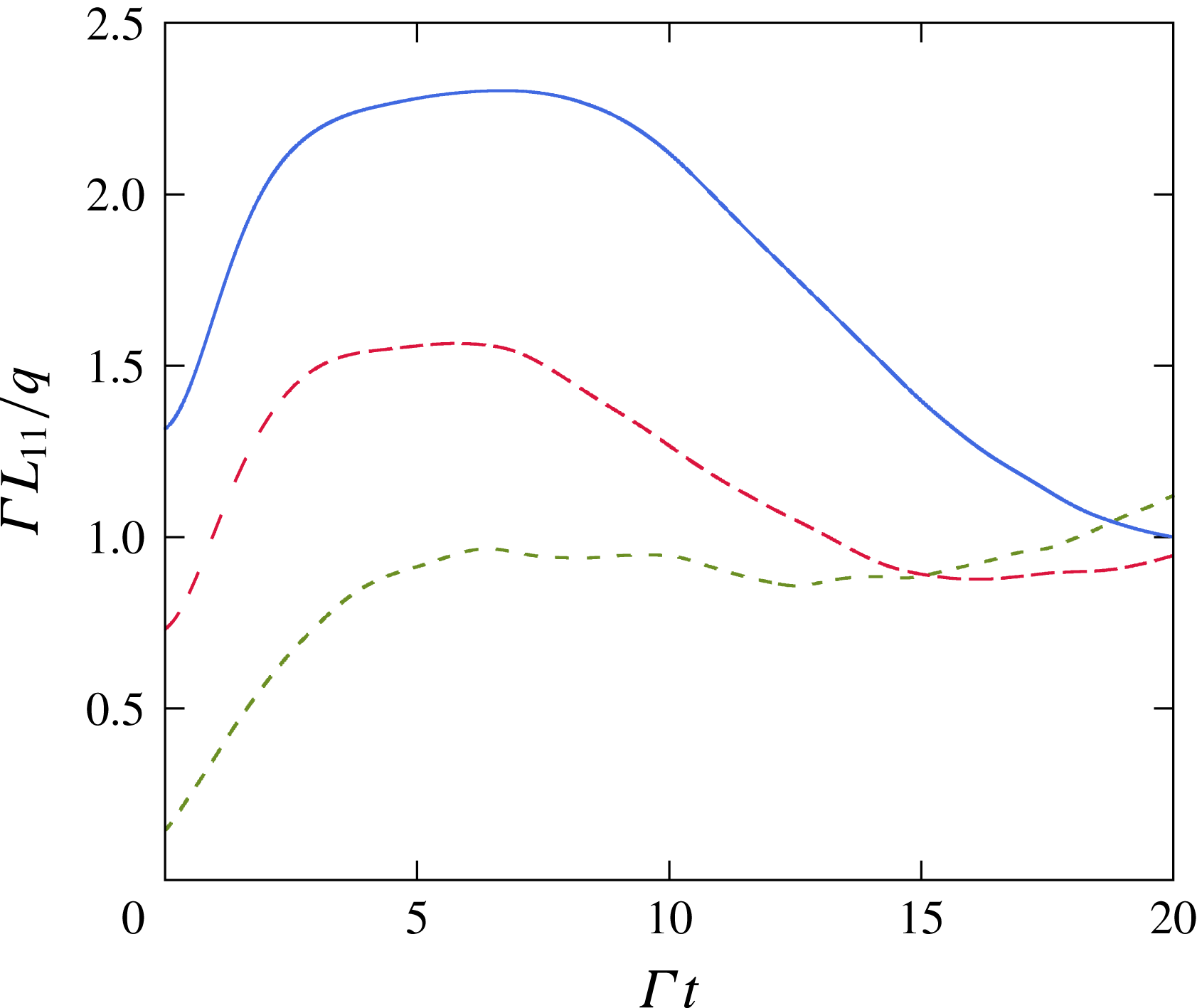
The integral length scale normalized by the characteristic large-scale length
 $q/\unicode[STIX]{x1D6E4}$
. The lines are as in figure 10.

To complete the analysis of the self-similar state, we plot the normalized integral length scale
 $\unicode[STIX]{x1D6E4}L_{11}/q$
in figure 12. Rogallo (Reference Rogallo1981) explained that this quantity must reach a non-zero plateau. On one hand, if
 $\unicode[STIX]{x1D6E4}L_{11}/q$
were to diverge, then the distortion terms would dominate at large times, leading to the ultimate decay of kinetic energy predicted by RDT (Rogallo Reference Rogallo1981; Rogers Reference Rogers1991). On the other hand, vanishing
 $\unicode[STIX]{x1D6E4}L_{11}/q$
implies a return to isotropy of the flow and decay of the kinetic energy as well. Consequently, the self-similar regime is characterized by constant
 $\unicode[STIX]{x1D6E4}L_{11}/q$
. Figure 12 suggests that this plateau is established around
 ${\sim}1$
for all three cases S03, S15 and S27.
4.3 Comparisons with viscous RDT
Here, we compare the short- and long-term turbulence statistics with predictions from viscous RDT. Previous researchers have also compared results with RDT. Rogers (Reference Rogers1991) provided early-time expansions of the inviscid RDT solution, valid until
 $\unicode[STIX]{x1D6E4}t\sim 1$
at very high shear rates. IC extended these expansions to the viscous case. They show a dependence on the shear number of the turbulence statistics that was absent from inviscid RDT. Comparisons with their DNS data were limited to the ratio
 ${\mathcal{P}}/\unicode[STIX]{x1D716}$
and showed qualitative agreement. DNS based on Rogallo’s method without remeshing by Lee et al. (Reference Lee, Kim and Moin1990) showed agreement with the inviscid linear theory at the high shear number
 $S_{0}^{\ast }=33.5$
until
 $\unicode[STIX]{x1D6E4}t=12$
. Here, we systematically compare the statistics discussed above with viscous RDT (
 $\unicode[STIX]{x1D708}$
RDT) introduced in IC. The Reynolds stresses
 $R_{ij}=\langle u_{i}u_{j}\rangle$
and dissipation rate
 $\unicode[STIX]{x1D716}$
from
 $\unicode[STIX]{x1D708}$
RDT are retrieved by computing the following integrals:
 $$\begin{eqnarray}\displaystyle R_{ij}(t) & = & \displaystyle \int \int \int \exp \left(-2\unicode[STIX]{x1D708}t\left(k^{2}-k_{x,0}k_{y,0}\unicode[STIX]{x1D6E4}t+\frac{(k_{x,0}\unicode[STIX]{x1D6E4}t)^{2}}{3}\right)\right)A_{ip}A_{jq}\unicode[STIX]{x1D719}_{pq}^{0}(\boldsymbol{k}_{0})\,\text{d}\boldsymbol{k}_{0},\end{eqnarray}$$
 $$\begin{eqnarray}\displaystyle \unicode[STIX]{x1D716}(t) & = & \displaystyle \unicode[STIX]{x1D708}\int \int \int k^{2}\exp \left(-2\unicode[STIX]{x1D708}t\left(k^{2}-k_{x,0}k_{y,0}\unicode[STIX]{x1D6E4}t+\frac{(k_{x,0}\unicode[STIX]{x1D6E4}t)^{2}}{3}\right)\right)A_{ip}A_{iq}\unicode[STIX]{x1D719}_{pq}^{0}(\boldsymbol{k}_{0})\,\text{d}\boldsymbol{k}_{0},\nonumber\\ \displaystyle & & \displaystyle\end{eqnarray}$$
where
 $\unicode[STIX]{x1D63C}$
is the RDT matrix defined in appendix A and
 $\unicode[STIX]{x1D719}_{ij}^{0}$
is the initial velocity spectrum,
 $$\begin{eqnarray}\unicode[STIX]{x1D719}_{ij}^{0}(\boldsymbol{k}_{0})=\frac{E_{0}(k_{0})}{4\unicode[STIX]{x03C0}k^{2}}\left(\unicode[STIX]{x1D6FF}_{ij}-\frac{k_{i,0}k_{j,0}}{k_{0}^{2}}\right).\end{eqnarray}$$
We evaluate the triple integral in spherical coordinates. The integral over wavenumber space, which is finite given the energy spectrum (4.1), is performed analytically to greatly reduce the computational cost. The integral over the azimuthal and polar angles is evaluated with a mid-point rule. All quantities presented here are computed on a mesh on the unit sphere refined until convergence. It should be noticed that a non-dimensionalization of time in the term
 $\exp (-2\unicode[STIX]{x1D708}t(\cdots \,))$
appearing in (4.4) and (4.5) reveals a factor
 $S^{\ast }q^{2}/Re^{2}$
. This, with the realization that the shear number does not appear in the RDT matrix, shows that only a viscous RDT approach accounts for differences arising from different shear numbers.
Figure 10 shows statistics computed from
 $\unicode[STIX]{x1D708}$
RDT alongside the DNS statistics for the medium-shear-number case S03 and the high-shear-number cases S15 and S27. We note first that the inclusion of viscous effects allows
 $\unicode[STIX]{x1D708}$
RDT to predict distinct evolution for the two cases considered. We observe that
 $\unicode[STIX]{x1D708}$
RDT matches the DNS data closely until
 $\unicode[STIX]{x1D6E4}t\sim 5$
. As expected,
 $\unicode[STIX]{x1D708}$
RDT matches the DNS data the best for the highest shear number, with the agreement for S03 being only qualitative. The viscous RDT matches the peak
 ${\mathcal{P}}/\unicode[STIX]{x1D716}$
and early transient in
 $S^{\ast }$
. The anisotropic stresses
 $\unicode[STIX]{x1D623}_{xx}$
,
 $\unicode[STIX]{x1D623}_{yy}$
,
 $\unicode[STIX]{x1D623}_{zz}$
and
 $\unicode[STIX]{x1D623}_{xy}$
from
 $\unicode[STIX]{x1D708}$
RDT, seen in figure 11, appear to have a similar time window of agreement with DNS, i.e.
 $0<\unicode[STIX]{x1D6E4}t<5$
. The evolution of these quantities predicted by
 $\unicode[STIX]{x1D708}$
RDT is marginally sensitive to the shear number.
The quality of the agreement for later times
 $\unicode[STIX]{x1D6E4}t>5$
quickly deteriorates for all cases and quantities considered. The anomalous behaviour of the long-time turbulence statistics from
 $\unicode[STIX]{x1D708}$
RDT is caused by the absence of nonlinear effects in the RDT model. It results in an approach that does not support the existence of a self-similar state as found in most experiments and as we find in our DNS. The kinetic energy from
 $\unicode[STIX]{x1D708}$
RDT grows linearly at large times (figure 10
b), contrary to the exponential growth expected. Rogers (Reference Rogers1991), using asymptotic expansion of inviscid RDT, already showed linear growth of the kinetic energy at long times. The breakdown of the approach is further seen from the anisotropic stresses, which tend towards
 $\unicode[STIX]{x1D623}_{xx}=2/3$
,
 $\unicode[STIX]{x1D623}_{yy}=\unicode[STIX]{x1D623}_{zz}=-1/3$
and
 $\unicode[STIX]{x1D623}_{xy}=0$
, corresponding to a monocomponent flow field (
 $u_{y}/u_{x}=u_{z}/u_{x}=0$
) (Lee et al.
Reference Lee, Kim and Moin1990).
IC suggested that the inclusion of a nonlinear model for the pressure strain might alleviate this issue. In the absence of such a solution, we find that
 $\unicode[STIX]{x1D708}$
RDT and our DNS at high shear numbers display satisfactory agreement until
 $\unicode[STIX]{x1D6E4}t\sim 5$
. It should be noted that the short-time expansion in IC was found to give acceptable results only until
 $\unicode[STIX]{x1D6E4}t\sim 1$
. Computation of the full
 $\unicode[STIX]{x1D708}$
RDT integrals allowed extension of this time range.
4.4 The transverse velocity derivative statistics
$\unicode[STIX]{x2202}u_{x}/\unicode[STIX]{x2202}y$

Homogeneously sheared turbulence has been central in the testing of one of the most celebrated turbulence theories. Kolmogorov’s theory of local isotropic turbulence is most famously known for the
 $-5/3$
scaling of the energy spectrum with wavenumber. The postulate states that the small scales become statistically homogeneous and isotropic when the Reynolds number is high enough. The theory is so successful that it has constituted the basis of a number of turbulence models and numerical methods. For instance, large-eddy simulations leverage the universality of the small scales to simplify the calculation to a numerical evaluation of the large scales only, considerably reducing the computational cost.
How large exactly this Reynolds number needs to be to achieve the isotropization of the small scales has been at the core of many experiments. It is argued that HST is particularly suited to test the local isotropy postulate. First, the widely studied homogeneous isotropic turbulence DNS and grid turbulence (nearly isotropic) are of limited use here. Second, general inhomogeneous flows (wake turbulence, turbulent jets, channel flows) studied in laboratory conditions or with DNS hardly achieve the stringent high Reynolds number required for true local isotropy. The absence of wall effects allows HST, in theory, to achieve izotropization of the small scales at lower
 $Re_{\unicode[STIX]{x1D706}}$
.
A consequence of the local isotropy postulate is that the odd moments of the transverse velocity derivative need to be zero in the limit of infinite Reynolds number (
 $Re_{\unicode[STIX]{x1D706}}\rightarrow \infty$
). Garg & Warhaft (Reference Garg and Warhaft1998), SW and Ferchichi & Tavoularis (Reference Ferchichi and Tavoularis2000) investigated experimentally the effect of the Reynolds number on the kurtosis and skewness of the transverse velocity derivative
 $\unicode[STIX]{x2202}u_{x}/\unicode[STIX]{x2202}y$
in HST. Garg & Warhaft (Reference Garg and Warhaft1998) considered longitudinal Taylor-microscale Reynolds numbers in the range
 $156\leqslant Re_{\unicode[STIX]{x1D706}_{xx}}\leqslant 390$
(
 ${\sim}112\leqslant Re_{\unicode[STIX]{x1D706}}\leqslant 280$
). Ferchichi & Tavoularis (Reference Ferchichi and Tavoularis2000) widened the range of Reynolds numbers studied to
 $140\leqslant Re_{\unicode[STIX]{x1D706}_{xx}}\leqslant 660$
, while SW were able to achieve the highest
 $Re_{\unicode[STIX]{x1D706}_{xx}}=1100$
. The numerical study in Isaza & Collins (Reference Isaza and Collins2011) explored the effects of the initial shear number
 $S_{0}^{\ast }$
on the moments of the velocity derivative over the range
 $22\leqslant Re_{\unicode[STIX]{x1D706}}\leqslant 68$
. In Boris et al. (Reference Boris, Luca, Gaetano and Carlo Massimo2004), Biferale & Procaccia (Reference Biferale and Procaccia2005), Casciola et al. (Reference Casciola, Gualtieri, Jacob and Piva2005) and Gualtieri et al. (Reference Gualtieri, Casciola, Jacob and Piva2007b
), the anisotropy of scales was analysed by decomposing the longitudinal structure function on the group of rotations SO(3). All of the past references concluded that, even at the highest
 $Re_{\unicode[STIX]{x1D706}}$
they considered, the flow still exhibited local anisotropy.
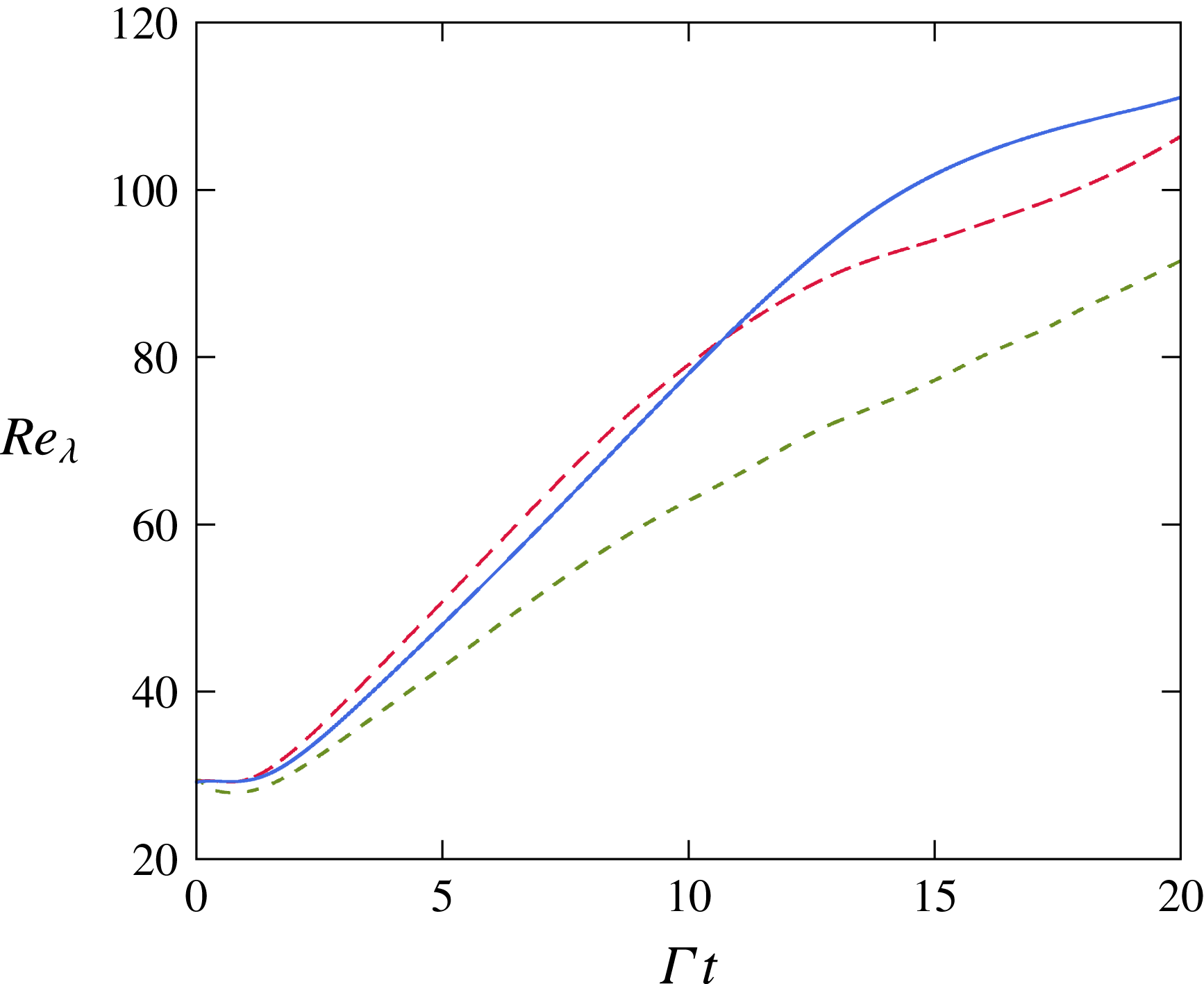
Evolution of the Taylor-microscale Reynolds number. The lines are as in figure 10.

Direct numerical simulation of HST for
 $Re_{\unicode[STIX]{x1D706}}$
of
 $O(10^{3})$
is unachievable with current computational resources and the resolution requirements discussed above. Figure 13 shows the evolution of the Reynolds number for the cases S03, S15 and S27. The maximum Reynolds number achieved was
 $Re_{\unicode[STIX]{x1D706}}=111$
for S27, followed by
 $Re_{\unicode[STIX]{x1D706}}=107$
for S15. It should be noticed that the Reynolds number grows at a similar rate for the high-shear-number cases S15 and S27 and a slower rate for S03. The upper bound of
 $Re_{\unicode[STIX]{x1D706}}$
in our simulations corresponds to the lower bound in the experiments cited above. Nevertheless, this allows us to compare S15 and S27 with the data of SW at
 $Re_{\unicode[STIX]{x1D706}_{xx}}=158$
(
 $Re_{\unicode[STIX]{x1D706}}\sim 107$
) and establish preliminary trends at low Reynolds numbers. The simulations also allow analysis of the effect of the initial shear number.
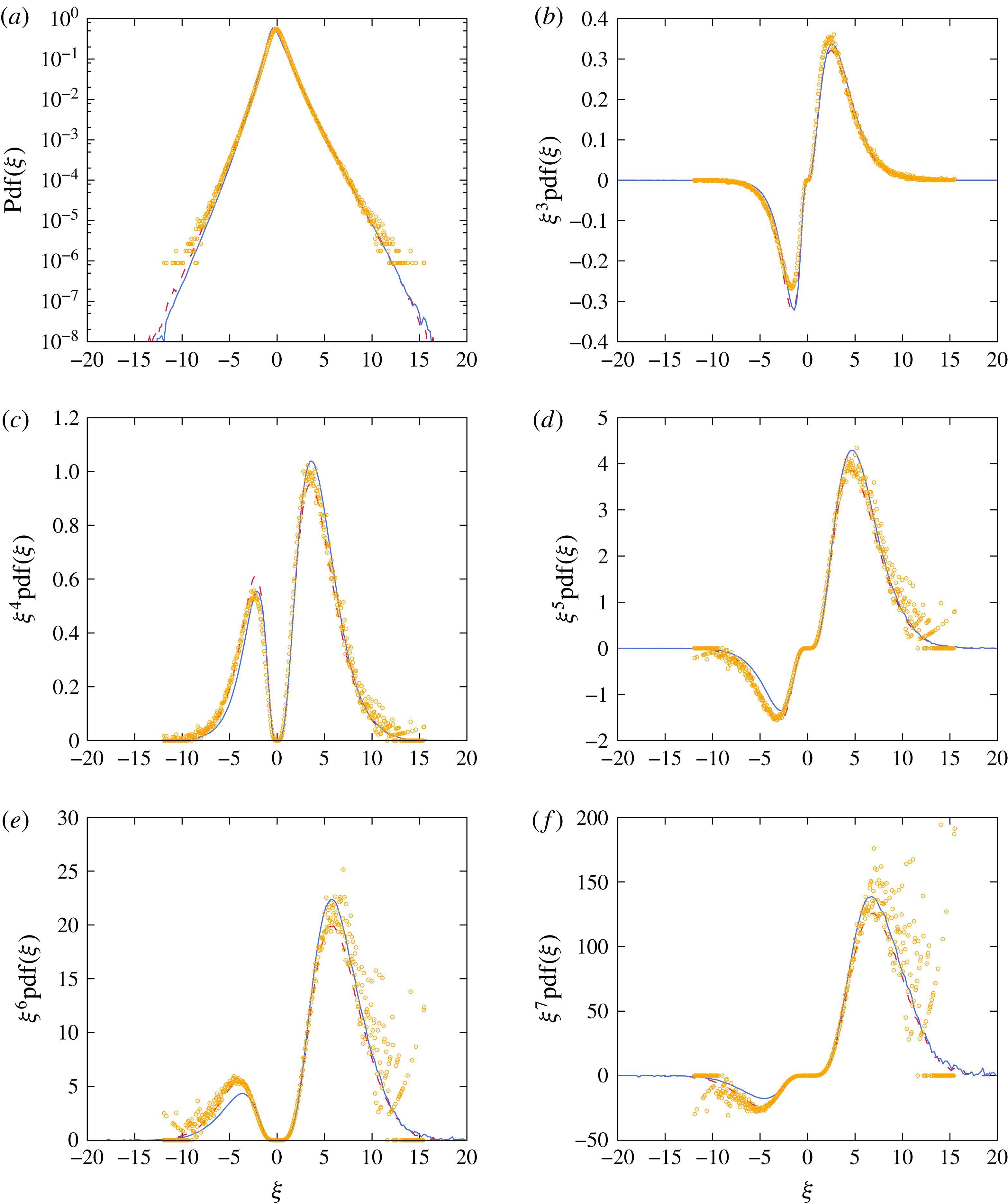
Figure 14(a) shows the probability density function (p.d.f.) of the normalized transverse velocity derivative,
 $$\begin{eqnarray}\unicode[STIX]{x1D709}=\frac{\unicode[STIX]{x2202}u_{x}/\unicode[STIX]{x2202}y}{\langle (\unicode[STIX]{x2202}u_{x}/\unicode[STIX]{x2202}y)^{2}\rangle ^{1/2}},\end{eqnarray}$$
at
 $Re_{\unicode[STIX]{x1D706}}=107$
. The two runs, S15 and S27, are reported alongside measurements by SW. The p.d.f.s are highly non-Gaussian and asymmetric. We observe a sharp peak shifted towards negative values and exponential tails. At this Reynolds number, cases S15 and S27 are essentially the same universal self-similar flow. They both yield great agreement with the data of SW, with S27 displaying a little more asymmetry of the p.d.f. and shorter tails. These small variations are likely to be caused by the slightly higher asymptotic shear number attained by S27 (see table 2).
The probability density function of the normalized transverse velocity derivative
 $\unicode[STIX]{x1D709}=(\unicode[STIX]{x2202}u_{x}/\unicode[STIX]{x2202}y)/\langle (\unicode[STIX]{x2202}u_{x}/\unicode[STIX]{x2202}y)^{2}\rangle ^{1/2}$
and the integrand for computing the moments of
 $\unicode[STIX]{x1D709}$
at
 $Re_{\unicode[STIX]{x1D706}}=107$
. The lines are as in figure 10. The symbol
 $\odot$
is from figure 9 in SW.

The integrands of the expressions for the moments of the p.d.f. of the normalized transverse velocity derivative,
 $\unicode[STIX]{x1D709}^{n}\text{pdf}(\unicode[STIX]{x1D709})$
, are reported in figure 14 for
 $n=3$
–7. Qualitatively, the agreement between the data of SW and the DNS holds well for all seven moments. The integrals of the odd orders
 $n=3$
, 5 and 7 from
 $-\infty$
to
 $+\infty$
correspond to the skewness
 $S_{3y}$
, superskewness
 $S_{5y}$
and hyperskewness
 $S_{7y}$
of the transverse velocity derivative
 $\unicode[STIX]{x2202}u_{x}/\unicode[STIX]{x2202}y$
. The integrals of the even orders
 $n=4$
and 6 are the kurtosis
 $K_{4y}$
and superkurtosis
 $K_{6y}$
. Due to experimental constraints, SW were able to measure only 18 standard deviations of the p.d.f. of
 $\unicode[STIX]{x1D709}$
, resulting in insufficient sampling for the computation of
 $K_{6y}$
and
 $S_{7y}$
. This is not an issue for DNS and shows how computational approaches might complete the information provided by experiments.
The transverse velocity derivative moments. (a) The skewness (bottom), superskewness (middle) and hyperskewness (top). (b) The kurtosis (bottom) and superkurtosis (top). The lines are as in figure 10.

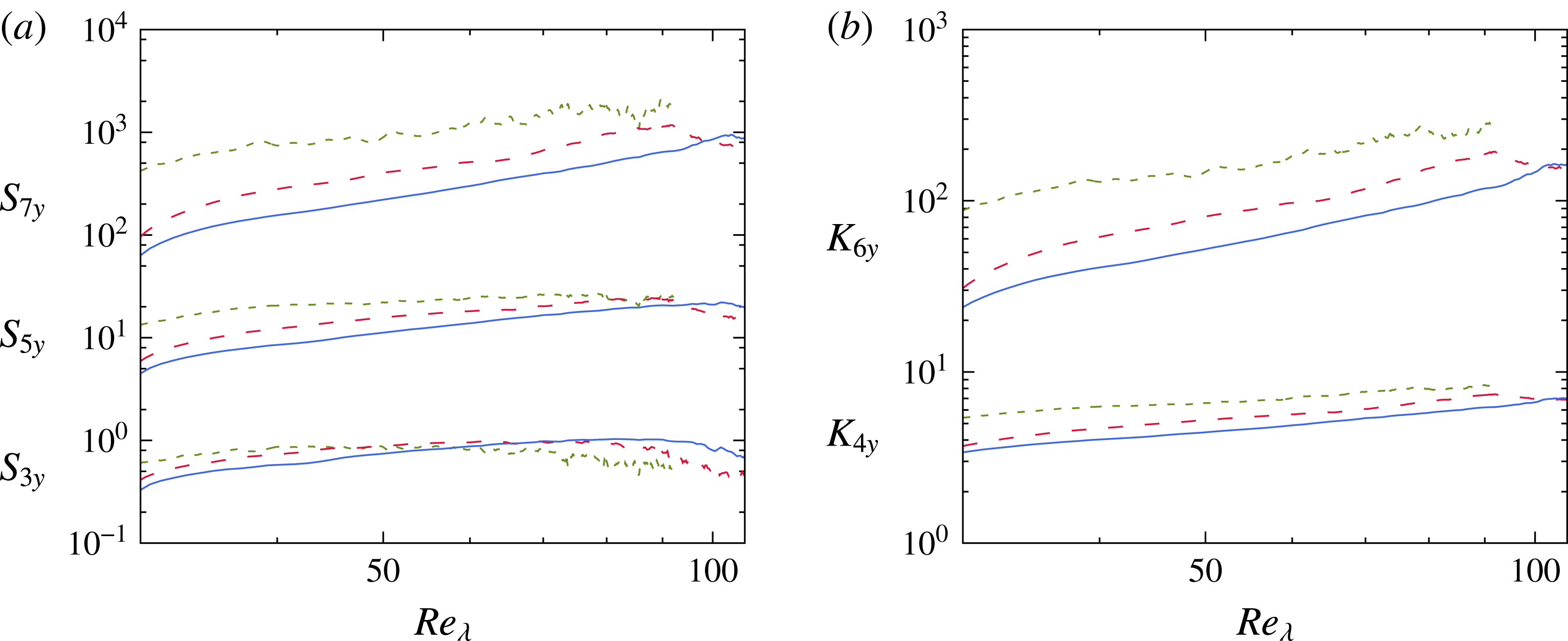
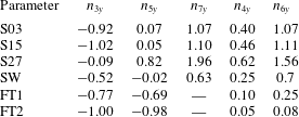
Figures 15(a) and 15(b) show the evolution with
 $Re_{\unicode[STIX]{x1D706}}$
of the odd and even moments respectively. In particular, at
 $Re_{\unicode[STIX]{x1D706}}=107$
, we find
 $S_{3y}=0.62$
,
 $S_{5y}=18.9$
,
 $S_{7y}=840$
,
 $K_{4y}=6.97$
and
 $K_{6y}=149$
from S27,
 $S_{3y}=0.46$
,
 $S_{5y}=15.5$
,
 $S_{7y}=716$
,
 $K_{4y}=6.88$
and
 $K_{6y}=153$
from S1. The data of SW yield
 $S_{3y}=0.6$
,
 $S_{5y}=16$
,
 $S_{7y}=860$
,
 $K_{4y}=7.2$
and
 $K_{6y}=175$
. It should be noted that the experimental uncertainty for the hyperskewness and superkurtosis is larger due to the undersampling discussed above. In light of this, the DNS displays close agreement with the experiment.
To test Kolmogorov’s postulate, it is customary to perform a fit of the data to a power law
 $ARe_{\unicode[STIX]{x1D706}}^{n}$
. Under Kolmogorov’s postulate of local isotropy,
 $n$
is negative for the odd moments (
 $n_{3y}$
,
 $n_{5y}$
,
 $n_{7y}$
) and positive for the even moments (
 $n_{4y}$
and
 $n_{6y}$
). To minimize the effects of the isotropic initial conditions, we perform the fit on our data for
 $Re_{\unicode[STIX]{x1D706}}>50$
. The exponents from our simulations and previous studies are reported in table 4.
The skewness
 $S_{3y}$
decreases for all three runs S03 and S15 and S27, although only slightly for the latter one. The differences in decay rate come from the initial period of growth of
 $S_{3y}$
due to the artificial initial conditions. The larger the initial shear number is, the more the moments are affected by the initial conditions. We note that the superskewness and hyperskewness have positive exponents, in contradiction to the local isotropy postulate. However, SW reported similar trends: decaying
 $S_{3y}$
, stagnating
 $S_{5y}$
and increasing
 $S_{7y}$
. The kurtosis and superkurtosis grow with increasing
 $Re_{\unicode[STIX]{x1D706}}$
as in Kolmogorov’s theory, albeit with stronger rates than in experiments.
The exponents in the power fit
 $Re_{\unicode[STIX]{x1D706}}^{n}$
of the transverse velocity derivative moments. Experiments: SW, Shen & Warhaft (Reference Shen and Warhaft2000); FT1 & FT2, Ferchichi & Tavoularis (Reference Ferchichi and Tavoularis2000).
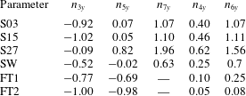
5 Conclusion
The development of algorithms capable of simulating homogeneously sheared flows enables the exploration of many physical questions. In this paper, we improve on the algorithm presented in Gerz et al. (Reference Gerz, Schumann and Elghobashi1989) and apply it to HST. The algorithm is based on a physical space formulation in the reference frame of the laboratory. This is in contrast to the formulation of Brucker et al. (Reference Brucker, Isaza, Vaithianathan and Collins2007) in Fourier space and the formulation of Rogallo (Reference Rogallo1981) in a moving reference frame. The former approach is subject to Gibbs oscillations at large total strains and the latter suffers from interpolation errors due to frequent remeshing and degradation of the cell aspect ratio. The method presented is stable and accurate and does not suffer from these problems.
Issues in the original method (Schumann Reference Schumann and Boujot1985; Schumann et al.
Reference Schumann, Elghobashi, Gerz, Schumann and Friedrich1986; Gerz et al.
Reference Gerz, Schumann and Elghobashi1989) have been addressed. An explicit time integration procedure that builds the
 $n+1$
update from
 $n$
states in conjunction with operator splitting for convection by the base shear term (see figure 6) allows the correct simulation of Kelvin modes (a ‘rotating’ wave that is a solution to the full Navier–Stokes equations) and stable simulations of HST. We present a Von Neumann analysis that explains why the use of an Adam–Bashforth integrator (1) distorts Kelvin modes and (2) leads to fast growing errors near the top and bottom boundaries,
 $y=\pm L_{y}/2$
.
We use the improved algorithm presented to simulate HST until a self-similar state is attained. For the initial Reynolds number
 $Re_{\unicode[STIX]{x1D706}0}=29$
and three different initial shear numbers
 $S_{0}^{\ast }=3$
, 15 and 27, we simulate until
 $\unicode[STIX]{x1D6E4}t=20$
on a
 $2048\times 1024\times 1024$
mesh. The large resolution is necessary to capture the smallest scales of the flow at all times, as they keep decreasing due to the mean shear motion. The simulation until
 $\unicode[STIX]{x1D6E4}t=20$
allows the observation of a self-similar state, reported in most experiments and characterized by (1) exponentially growing turbulent kinetic energy, (2) plateauing of the turbulence statistics when non-dimensionalized by the shear rate (shear number
 $S^{\ast }$
, ratio of production to dissipation
 ${\mathcal{P}}/\unicode[STIX]{x1D716}$
, anisotropic Reynolds stresses
 $\unicode[STIX]{x1D623}_{ij}$
) and (3) plateauing of the integral length scale non-dimensionalized by the shear rate and kinetic energy. Comparisons with the experiments of Tavoularis & Corrsin (Reference Tavoularis and Corrsin1981) and Shen & Warhaft (Reference Shen and Warhaft2000) show excellent agreement.
The three runs show that the self-similar states achieved are almost independent of the initial shear number
 $S_{0}^{\ast }$
. Most notably, we find the asymptotic values
 $S^{\ast }\sim 10$
,
 ${\mathcal{P}}/\unicode[STIX]{x1D716}\sim 1.5$
and
 $\unicode[STIX]{x1D623}_{xy}\sim -0.14$
. Experiments under different operating conditions (table 2) report values close to the ones we find. This suggests that the self-similar state is universal and is independent of the initial shear number and Reynolds number.
Comparisons with
 $\unicode[STIX]{x1D708}$
RDT (Isaza & Collins Reference Isaza and Collins2009) show good agreement until
 $\unicode[STIX]{x1D6E4}t\sim 5$
. As expected from this linear theory, the agreement deteriorates with diminishing initial shear number. The long-time statistics of RDT (
 $\unicode[STIX]{x1D6E4}t>5$
) differ significantly from those found in simulations and experiments because of the absence of all nonlinearities. These terms have a cumulative effect which leads to the exponential growth of kinetic energy and the appearance of a self-similar state. In contrast, RDT displays linear growth of the kinetic energy and long-time statistics that depend sensitively on the initial shear number.
For the initial non-dimensional numbers considered, the small scales display significant anisotropy. The probability density function of the transverse velocity derivative,
 $\unicode[STIX]{x2202}u_{x}/\unicode[STIX]{x2202}y$
, shows qualitative and quantitative agreement with the one measured by Shen & Warhaft (Reference Shen and Warhaft2000) at
 $Re_{\unicode[STIX]{x1D706}}=107$
. The evolution of the third, fifth and seventh moments,
 $S_{3y}$
,
 $S_{5y}$
and
 $S_{7y}$
, indicates that local isotropization of scales, if it occurs at all, requires significantly higher Reynolds numbers than the one considered,
 $29\leqslant Re_{\unicode[STIX]{x1D706}}\leqslant 111$
. Despite growing super- and hyperskewnesses with Reynolds number, the skewness
 $S_{3y}$
is seen to decrease. This trend is similar to what is reported in experiments. We also find that the degree of anisotropy increases with increasing initial shear number.
Appendix A. The rapid distortion matrix
In the context of RDT, a Fourier mode with the initial wavevector
 $\boldsymbol{k}(t=0)=\boldsymbol{k}_{0}=(k_{x,0},k_{y,0},k_{z,0})$
is turned by the base homogeneous shear flow
 $\boldsymbol{u}_{b}$
according to
 $$\begin{eqnarray}\frac{\text{d}\boldsymbol{k}}{\text{d}t}=\unicode[STIX]{x1D735}\boldsymbol{u}_{b}\boldsymbol{\cdot }\boldsymbol{k}.\end{eqnarray}$$
When the shear gradient is in the
 $y$
direction and the shear rate is
 $\unicode[STIX]{x1D6E4}$
,
 $\boldsymbol{u}_{b}=y\unicode[STIX]{x1D6E4}\boldsymbol{e}_{x}$
, the components
 $x$
and
 $z$
of the wavevector remain constant whereas
 $$\begin{eqnarray}k_{y}=k_{y,0}-k_{x}\unicode[STIX]{x1D6E4}t.\end{eqnarray}$$
In addition to the change of orientation and wavelength incurred by the variation of
 $\boldsymbol{k}$
, the amplitude of the Fourier mode evolves following
 $$\begin{eqnarray}\hat{\boldsymbol{u}}(t)=\unicode[STIX]{x1D63C}(\boldsymbol{k}_{0},t)\hat{\boldsymbol{u}}_{0}\exp \left(-\unicode[STIX]{x1D708}t\left(k^{2}-k_{x,0}k_{y,0}\unicode[STIX]{x1D6E4}t+\frac{(k_{x,0}\unicode[STIX]{x1D6E4}t)^{2}}{3}\right)\right),\end{eqnarray}$$
where
 $\boldsymbol{u}_{0}$
is the initial amplitude,
 $\unicode[STIX]{x1D708}$
is the kinematic viscosity and
 $\unicode[STIX]{x1D63C}$
is the RDT matrix,
 $$\begin{eqnarray}\displaystyle \unicode[STIX]{x1D63C}(\boldsymbol{k}_{0},t) & = & \displaystyle \left(\begin{array}{@{}ccc@{}}1 & {\displaystyle \frac{k_{0}^{2}}{k_{x}^{2}+k_{z}^{2}}}\left(-{\displaystyle \frac{k_{z}^{2}}{k_{0}^{2}}}P+{\displaystyle \frac{k_{x}^{2}}{k_{0}^{2}}}Q\right) & 0\\ 0 & {\displaystyle \frac{k_{0}^{2}}{k^{2}}} & 0\\ 0 & {\displaystyle \frac{k_{x}k_{z}}{k_{x}^{2}+k_{z}^{2}}}(P+Q) & 1\end{array}\right),\end{eqnarray}$$
 $$\begin{eqnarray}\displaystyle P & = & \displaystyle {\displaystyle \frac{k_{0}^{2}}{k_{x}\sqrt{k_{x}^{2}+k_{z}^{2}}}}(\arctan \unicode[STIX]{x1D6FC}-\arctan \unicode[STIX]{x1D70F}),\end{eqnarray}$$
 $$\begin{eqnarray}\displaystyle Q & = & \displaystyle {\displaystyle \frac{\unicode[STIX]{x1D6E4}t(k_{0}^{2}-2k_{y,0}^{2}+k_{x}k_{y,0}\unicode[STIX]{x1D6E4}t)}{k^{2}}},\end{eqnarray}$$
 $$\begin{eqnarray}\displaystyle \unicode[STIX]{x1D6FC} & = & \displaystyle {\displaystyle \frac{k_{y,0}}{\sqrt{k_{x}^{2}+k_{z}^{2}}}},\end{eqnarray}$$
 $$\begin{eqnarray}\displaystyle \unicode[STIX]{x1D70F} & = & \displaystyle {\displaystyle \frac{k_{y}}{\sqrt{k_{x}^{2}+k_{z}^{2}}}}.\end{eqnarray}$$