1 Introduction
This paper experimentally investigates the enstrophy dynamics in turbulent premixed swirl flames, such as those often used in gas turbine engines. The enstrophy is defined as
 $\unicode[STIX]{x1D6FA}=\unicode[STIX]{x1D714}_{i}\unicode[STIX]{x1D714}_{i}$
, where
 $\unicode[STIX]{x1D714}_{i}$
is the vorticity. Specifically, we address the question of whether there is significant production of enstrophy due to the simultaneous action of the swirling flow and the flame.
The enstrophy transport equation is
 $$\begin{eqnarray}\frac{1}{2}\underbrace{\left(\frac{\unicode[STIX]{x2202}\unicode[STIX]{x1D6FA}}{\unicode[STIX]{x2202}t}+u_{i}\frac{\unicode[STIX]{x2202}\unicode[STIX]{x1D6FA}}{\unicode[STIX]{x2202}x_{i}}\right)}_{L}=\underbrace{\unicode[STIX]{x1D714}_{i}\unicode[STIX]{x1D714}_{j}\frac{\unicode[STIX]{x2202}u_{i}}{\unicode[STIX]{x2202}x_{j}}}_{I}-\underbrace{\unicode[STIX]{x1D6FA}\frac{\unicode[STIX]{x2202}u_{k}}{\unicode[STIX]{x2202}x_{k}}}_{II}+\underbrace{\frac{1}{\unicode[STIX]{x1D70C}^{2}}\unicode[STIX]{x1D714}_{i}\unicode[STIX]{x1D700}_{ijk}\frac{\unicode[STIX]{x2202}\unicode[STIX]{x1D70C}}{\unicode[STIX]{x2202}x_{j}}\frac{\unicode[STIX]{x2202}p}{\unicode[STIX]{x2202}x_{k}}}_{III}+\underbrace{\unicode[STIX]{x1D714}_{i}\unicode[STIX]{x1D700}_{ijk}\frac{\unicode[STIX]{x2202}}{\unicode[STIX]{x2202}x_{j}}\left(\frac{1}{\unicode[STIX]{x1D70C}}\frac{\unicode[STIX]{x2202}\unicode[STIX]{x1D70F}_{km}}{\unicode[STIX]{x2202}x_{m}}\right)}_{IV},\end{eqnarray}$$
where
 $\unicode[STIX]{x1D70F}_{ij}$
is the viscous stress tensor and
 $\unicode[STIX]{x1D700}_{ijk}$
is the cyclic permutation tensor.
 $L$
is the Lagrangian derivative of
 $\unicode[STIX]{x1D6FA}$
. The terms
 $I$
,
 $II$
and
 $III$
represent the effects of vortex stretching, dilatation and baroclinic torque, respectively. Term
 $IV$
represents the combination of diffusive transport and viscous dissipation of enstrophy.
Only terms
 $I$
and
 $IV$
are active in constant density non-reacting turbulence, leading to enstrophy concentrating at a scale that is
 $O(10)\unicode[STIX]{x1D702}$
where these effects balance (Buch & Dahm Reference Buch and Dahm1998). Here,
 $\unicode[STIX]{x1D702}$
denotes the Kolmogorov length scale. Combustion complicates the enstrophy dynamics by introducing dilatation and baroclinic torque effects, as well as variations in
 $\unicode[STIX]{x1D70F}_{ij}$
due to the dependence of viscosity on temperature. Combustion also influences vortex stretching by dilatation and adjusting the relative alignment of the vorticity and rate-of-strain tensor (e.g. Hamlington, Poludnenko & Oran Reference Hamlington, Poludnenko and Oran2011; Steinberg, Driscoll & Swaminathan Reference Steinberg, Driscoll and Swaminathan2012; Chakraborty Reference Chakraborty2014; Coriton & Frank Reference Coriton and Frank2017; MacArt, Grenga & Mueller Reference MacArt, Grenga and Mueller2018).
If
 $II$
and
 $III$
are significant contributors to enstrophy transport (i.e.
 $L$
) relative to
 $I$
and
 $IV$
, the presence of the flame plays an active role in the turbulence dynamics at the length scales of the flame (viz. the laminar flame thermal thickness
 $\unicode[STIX]{x1D6FF}_{l}^{0}$
). This would influence both the flame scale turbulence/scalar interactions – which are critical for understanding the volumetric burning rate – and the turbulence downstream of the flame. Since the influence of the flame is to produce
 $\unicode[STIX]{x2202}_{k}u_{k}>0$
, dilatation acts purely as an enstrophy sink; flame-generated enstrophy is attributed solely to baroclinic torque.
There have been numerous studies regarding the influence of the flame on vorticity (e.g. Renard et al. Reference Renard, Thévenin, Rolon and Candel2000). Early experimental and numerical work often used the idealized framework of isolated two-dimensional vortices interacting with a planar flame front (Louch & Bray Reference Louch and Bray1998; Mueller et al. Reference Mueller, Driscoll, Reuss, Drake and Rosalik1998). These studies demonstrated attenuation of reactant side vorticity and subsequent generation of product side vorticity with opposite sign due to baroclinic torque.
Recently, direct numerical simulations (DNS) have been used extensively to study enstrophy transport in the canonical configuration of flames embedded in boxes of low Mach number homogeneous isotropic turbulence (HIT) (Bobbitt & Blanquart Reference Bobbitt and Blanquart2016; Bobbitt, Lapointe & Blanquart Reference Bobbitt, Lapointe and Blanquart2016; Chakraborty, Konstantinou & Lipatnikov Reference Chakraborty, Konstantinou and Lipatnikov2016; Dopazo, Cifuentes & Chakraborty Reference Dopazo, Cifuentes and Chakraborty2017; Papapostolou et al.
Reference Papapostolou, Wacks, Chakraborty, Klein and Im2017). Bobbitt et al. (Reference Bobbitt, Lapointe and Blanquart2016) showed that, at sufficiently high Karlovitz number (
 $Ka=(\unicode[STIX]{x1D6FF}_{l}^{0}/\unicode[STIX]{x1D702})^{2}$
), both vortex stretching and dissipation follow the same scaling as in non-reacting HIT, viz.
 $I\propto IV\propto \unicode[STIX]{x1D70F}_{\unicode[STIX]{x1D702}}^{-3}$
, where
 $\unicode[STIX]{x1D70F}_{\unicode[STIX]{x1D702}}$
is the Kolmogorov time scale. This scaling held at their lowest turbulence intensity, corresponding to
 $Ka=70$
and
 $Re_{T}=u^{\prime }\ell /\unicode[STIX]{x1D708}_{r}=83$
, where
 $u^{\prime }$
is the root-mean-squared velocity oscillation,
 $\ell$
is the integral scale and
 $\unicode[STIX]{x1D708}_{r}$
is the kinematic viscosity of the reactants.
Regarding the baroclinic torque, pressure gradients in turbulent flames may arise due to both the flame and motion of the fluid. Flame pressure gradients scale as
 $\unicode[STIX]{x1D70C}s_{T}^{2}/\unicode[STIX]{x1D6FF}_{T}$
, where
 $s_{T}$
is the turbulent burning velocity and
 $\unicode[STIX]{x1D6FF}_{T}$
is the flame brush thickness, while pressure gradients induced by vortical motion at length scale
 $l$
and rotational velocity
 $u_{l}$
scale as
 $\unicode[STIX]{x1D70C}u_{l}^{2}/l$
. For incompressible HIT and assuming
 $s_{T}^{2}/\unicode[STIX]{x1D6FF}_{T}\approx {s_{l}^{0}}^{2}/\unicode[STIX]{x1D6FF}_{l}^{0}$
, Bobbitt et al. (Reference Bobbitt, Lapointe and Blanquart2016) showed that the pressure gradients are dominated by Kolmogorov scale vortical motions, that is,
 $|\unicode[STIX]{x1D6FB}p|\propto \unicode[STIX]{x1D70C}u_{\unicode[STIX]{x1D702}}^{2}/\unicode[STIX]{x1D702}$
, where
 $u_{\unicode[STIX]{x1D702}}=\unicode[STIX]{x1D702}/\unicode[STIX]{x1D70F}_{\unicode[STIX]{x1D702}}$
is the Kolmogorov velocity scale. In this case, although
 $III$
increased with turbulence intensity, it decreased in significance as compared to
 $I$
and
 $IV$
. Hence, the enstrophy dynamics were dominated by vortex stretching and dissipation; the primary effect of the flame was to increase the viscosity in the products.
However, this conclusion relies on the pressure gradients being dominated by those arising from Kolmogorov scale rotational motion. Many situations exist in which this may not hold, such as flames with high
 $s_{T}$
(e.g. approaching the Chapman–Jouget deflagration limit) or in flows that induce large-scale pressure gradients. The former has been proposed as part of the mechanism by which flames self-accelerate in unconfined media (Poludnenko, Gardiner & Oran Reference Poludnenko, Gardiner and Oran2011; Poludnenko Reference Poludnenko2015). The importance of the latter has recently been demonstrated in the case of low Reynolds number bluff-body-stabilized flames embedded in converging (nozzle), constant area and diverging (diffuser) ducts; the nozzle and diffuser configurations showed enhancement and attenuation, respectively, of the product side vorticity relative to the neutral configuration (Geikie et al.
Reference Geikie, Carr, Ahmed and Forliti2017; Geikie & Ahmed Reference Geikie and Ahmed2018). While experimental enstrophy budgets were calculated in Geikie & Ahmed (Reference Geikie and Ahmed2018), the analysis did not consider three-dimensional (3-D) effects or term
 $IV$
.
Swirling flows are important in numerous combustion devices and induce large-scale pressure fields with gradients in the axial and radial directions. Ishizuka (Reference Ishizuka2002) describes how the low density of the burnt products results in a weaker centrifugal force in the products compared to the higher density reactants and, consequently, a static pressure increase across the flame that scales as
 $\unicode[STIX]{x0394}p\propto \unicode[STIX]{x1D70C}_{r}u_{\unicode[STIX]{x1D703},max}^{2}(1-\unicode[STIX]{x1D70C}_{p}\unicode[STIX]{x1D70C}_{r}^{-1})$
, where
 $u_{\unicode[STIX]{x1D703},max}$
is the maximum tangential velocity. This increase in static pressure contrasts with the pressure decrease found in non-swirling deflagrations, which arises from the conversion of static pressure to momentum. Hence, baroclinic torque may contribute significantly to the enstrophy dynamics in turbulent swirl flames beyond what may be expected from flames in low-speed HIT at comparable turbulence intensities.
The main objective of this work therefore was to quantify the various terms in (1.1) for swirling flames using high-resolution tomographic particle image velocimetry (T-PIV), which is combined with planar laser induced fluorescence (PLIF) of formaldehyde (
 $\text{CH}_{2}\text{O}$
) to describe the flame structure and estimate mixture viscosity within the flame.
2 Experiment and diagnostics
2.1 Combustor and operating conditions
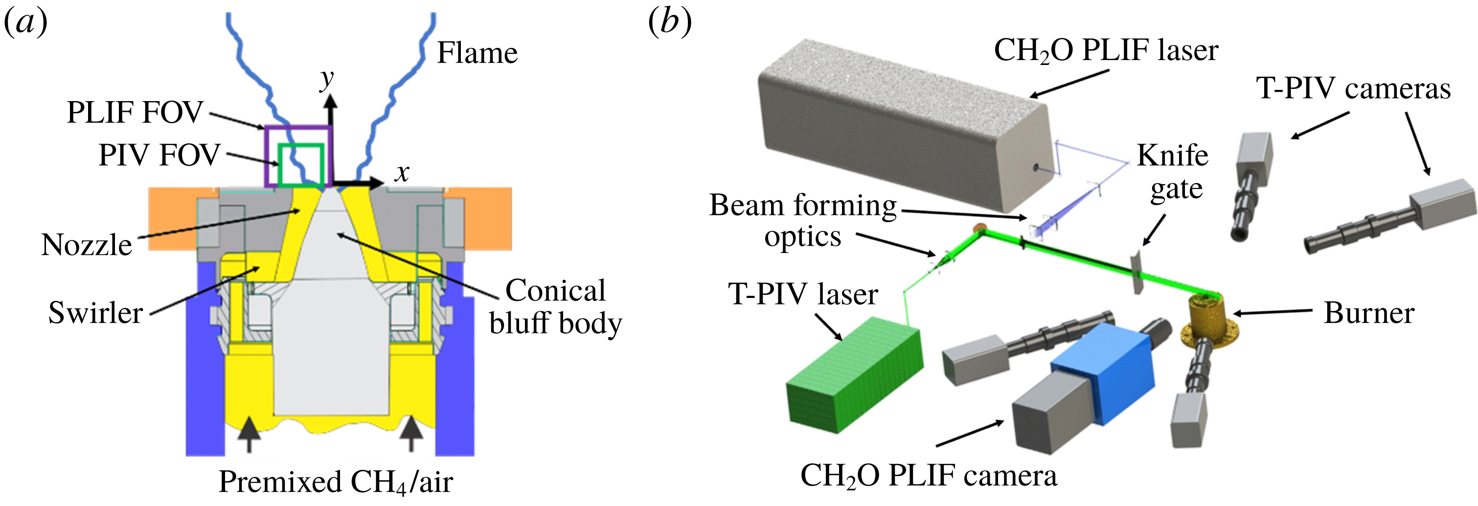
Experimental set-up showing (a) the swirl combustor and (b) the laser diagnostic set-up.

The swirl combustor used in this work (figure 1
a) was similar to that described by Meier et al. (Reference Meier, Weigand, Duan and Giezendanner-Thoben2007), but was operated with perfectly premixed reactants as in Caux-Brisebois et al. (Reference Caux-Brisebois, Steinberg, Arndt and Meier2014) and without the combustion chamber to prevent window contamination due to T-PIV seed particles. Ambient temperature reactants (methane (CH
 $_{4}$
) and air) were metered using electromechanical mass flow controllers (Brooks) and mixed approximately 2 m upstream of the combustor plenum. Swirl was induced by a 12-vane radial swirler, with a measured swirl number of 0.55 at the exit of the
 $D_{e}=27.85~\text{mm}$
diameter nozzle. The inner surface of the nozzle was formed by a conical bluff body with a spherical tip.
The test conditions are summarized in table 1. Here,
 $\unicode[STIX]{x1D719}$
is the equivalence ratio,
 $U$
is the bulk-velocity (i.e. the ratio of the total volumetric flow rate and nozzle exit area) and the jet Reynolds number is
 $Re_{j}=UD_{e}/\unicode[STIX]{x1D708}_{r}$
. The laminar flame properties were calculated using Cantera with the GRI3.0 chemical mechanism.
 $Re_{T}$
was calculated based on
 $u^{\prime }$
at the centre of the nozzle exit. We note that neither
 $\unicode[STIX]{x1D702}$
nor
 $Ka$
are included in table 1 due to the difficulty in defining these in this highly inhomogeneous system. Estimates for
 $\unicode[STIX]{x1D702}$
based on
 $\ell \approx D_{e}/2$
and
 $\unicode[STIX]{x1D702}\approx \ell Re_{T}^{-3/4}$
yield
 $\unicode[STIX]{x1D702}\approx 35{-}45~\unicode[STIX]{x03BC}\text{m}$
.
Test conditions and turbulence properties for each case.

2.2 Diagnostics
Measurements were made using simultaneous T-PIV and
 $\text{CH}_{2}\text{O}$
PLIF (figure 1
b). A total of 1000 T-PIV and PLIF measurements were made at each reacting condition. Furthermore, an additional 1000 T-PIV measurements were made for the equivalent non-reacting flow condition for each case. In each non-reacting case, the air flow rate was increased appropriately to match the total volumetric flow rate of the air and fuel of the corresponding reacting case.
2.2.1 Tomographic PIV
The T-PIV system consisted of a Nd:YAG laser (Quantel Evergreen 200, 532 nm, 10 Hz,
 $200~\text{mJ}~\text{pulse}^{-1}$
) and four sCMOS cameras (Andor Zyla 5.5,
 $2048\times 2048~\text{pixels}$
,
 $6.5~\unicode[STIX]{x03BC}\text{m}$
pixel length). Cylindrical lenses vertically expanded and collimated the laser beam at a height of 25 mm. This beam was formed into a collimated slab with a width of approximately 1.3 mm by passing it through a slit comprised of two knife edges. The time delay between laser pulse pairs was varied, depending on conditions, to allow sufficient particle displacement between frames for accurate velocity calculation.
The diagnostics were fine-tuned to balance the diffraction-limited particle image size, depth of field, particle density and interrogation volume size. The flow was seeded with aluminium oxide (
 $\text{Al}_{2}\text{O}_{3}$
) particles with a nominal diameter of
 $0.3~\unicode[STIX]{x03BC}\text{m}$
, which corresponds to a Stokes number – based on a conservative estimate of the Kolmogorov time scale – below 0.03 for all test cases. Mie scattering from seeding particles was simultaneously imaged by the four sCMOS cameras, operated at 20 Hz in a frame-straddling mode. The cameras were positioned on both sides of the laser sheet, at angles varying between
 $20^{\circ }$
and
 $30^{\circ }$
relative to the laser propagation direction. The cameras were equipped with long-distance microscopes (Infinity K2, CF-1/B objectives) and Scheimpflug mounts (LaVision) to prevent image blurring due to the off-axis viewing angle. The microscopes were operated at a numerical aperture of 0.013 – corresponding to
 $f/\#=38$
– to obtain the necessary depth of field across the probe volume, which was approximately
 $16\times 16\times 1.3~\text{mm}^{3}$
.
Velocity fields were calculated by spatial cross-correlation using an adaptive evaluation algorithm in a commercial software package (LaVision DaVis 8.4). Processing of the 3-D velocity fields consisted of camera volume calibration, preprocessing of particle images, camera self-calibration, reconstruction of 3-D particle fields, velocity field estimation via cross-correlation of the resulting tomogram pairs, and post-processing. A final interrogation volume length of 32 voxels (vx) was used with an overlap of 50 % (see § 3.2), resulting in a
 $250~\unicode[STIX]{x03BC}\text{m}$
interrogation box size and
 $125~\unicode[STIX]{x03BC}\text{m}$
vector spacing. A universal outlier detection, removal and insertion algorithm was used to reduce spurious vectors. Ghost particle levels were calculated by examining the
 $z$
-profile intensity and estimated to be 16–25 % between all cases. The data were smoothed using the penalized least-squares method of Garcia (Reference Garcia2010) with a smoothing parameter of 0.5.
2.2.2 CH
 $_{2}$
O PLIF

In
 $\text{CH}_{4}$
/air flames,
 $\text{CH}_{2}\text{O}$
is produced during the initial fuel breakdown reactions and is rapidly consumed during the formation of HCO at the final stages of oxidation. As such,
 $\text{CH}_{2}\text{O}$
PLIF is an indicator of the overall width of the instantaneous flame; the product side of the
 $\text{CH}_{2}\text{O}$
PLIF signal corresponds to regions of rapid heat release (Najm et al.
Reference Najm, Knio, Paul and Wyckoff1998; Wabel et al.
Reference Wabel, Zhang, Zhao, Wang, Hawkes and Steinberg2018). The
 $\text{CH}_{2}\text{O}$
PLIF system consisted of a Nd:YAG laser (Quanta-Ray INDI-40-10, 355 nm, 10 Hz,
 $70~\text{mJ}~\text{pulse}$
) and a sCMOS camera (Andor Neo 5.5,
 $2048\times 2048~\text{pixels}$
,
 $6.5~\unicode[STIX]{x03BC}\text{m}$
pixel length) coupled to an image intensifier (LaVision IRO,
 $\text{gate}=100~\text{ns}$
) and camera lens (Tamron,
 $f=180~\text{mm}$
,
 $f/\#=2.8$
). The laser excited the
 $A-X_{0}^{1}$
transition of
 $\text{CH}_{2}\text{O}$
in a bandwidth around 355 nm. The laser sheet was formed by cylindrical optics to a height of 30 mm and full-width at half-maximum of
 $100~\unicode[STIX]{x03BC}\text{m}$
and then transmitted along the centre of the T-PIV volume. Images were taken with a field of view of
 $20\times 20~\text{mm}$
, overlapping the
 $x$
-
 $y$
domain of the T-PIV at
 $z=0$
. Fluorescence from
 $\text{CH}_{2}\text{O}$
in the range of 370–480 nm was isolated using a specialized filter (Semrock FF01-CH2O-50.8-D).
3 Data processing and uncertainty
3.1 Overview
All of the analysis below is performed at the central plane of the T-PIV volume, corresponding to the locations of the PLIF measurements. We consider the Reynolds-averaged version of (1.1), viz.
 $$\begin{eqnarray}{\textstyle \frac{1}{2}}\overline{L}=\overline{I}-\overline{II}+\overline{III}+\overline{IV},\end{eqnarray}$$
where
 $\overline{L}=\overline{u_{j}\unicode[STIX]{x2202}_{j}\unicode[STIX]{x1D6FA}}$
represents the mean turbulent advection in this statistically steady flow. Because the flow was statistically stationary, the Reynolds averaging was performed by ensemble averaging. The mean vortex stretching
 $\overline{I}$
, dilatation
 $\overline{II}$
and advection
 $\overline{L}$
can be determined directly from well-resolved velocity measurements. However,
 $\overline{III}$
could not be measured, as it requires knowledge of both the pressure and density fields; our general approach will be to determine
 $\overline{III}$
as the difference between
 $\overline{L}$
and the other terms on the right-hand side of (3.1). We note here that the measurement of
 $\overline{IV}$
is challenging as it requires calculation of third spatial derivatives of the velocity field, as well as measurements of the fluid density and fluid viscosity, which are temperature dependent.
The analysis presented below therefore progresses in two steps. We first consider the sum
 $(\overline{III}+\overline{IV})_{L}=\frac{1}{2}\overline{L}-\overline{I}+\overline{II}$
. Here, the subscript
 $(\cdot )_{L}$
indicates that the term on the left is calculated by subtracting appropriate terms from the Lagrangian term. We compare the shapes of the
 $(\overline{III}+\overline{IV})_{L}$
curves in the reacting case to the
 $\overline{IV}_{L}=\frac{1}{2}\overline{L}-\overline{I}$
curves in the non-reacting case in order to describe qualitative differences. This analysis can be performed based on the T-PIV data alone. We then provide our best estimate of
 $\overline{IV}$
in the reacting cases by direct calculation using the T-PIV and PLIF data, thus allowing calculation of
 $\overline{III}_{L}=\frac{1}{2}\overline{L}-\overline{I}+\overline{II}-\overline{IV}$
. Uncertainty in all calculations is discussed below.
In order to compare (i) data at different axial locations
 $y$
in a given case, (ii) data from different cases and (iii) data from the non-reacting versus reacting conditions, it is necessary to reference the spatial location against physically meaningful locations in the system. To do so, we segment the data into 2 mm tall bands. Within each band, we plot the various quantities of interest against radial position
 $x$
, centred about the position
 $x_{0}$
that corresponds to the maximum
 $\overline{I}$
in that band. It was found that the profiles at different heights and conditions collapsed well in this coordinate system. To further facilitate comparison across different cases, we also present averages across all axial locations within a case. We denote these averaged results by
 $\langle \cdot \rangle$
.
3.2 Velocity uncertainty and resolution
Uncertainty in the measurement of the velocity field and its gradients arises due to both measurement noise and under-resolution. Uncertainty in the mean quantities of interest arises due to these sources and statistical convergence. Measurement noise is associated with a random uncertainty that reduces the convergence rate by artificially increasing the variance. The resultant uncertainty in the mean quantities that are calculated directly from the velocity measurements (e.g.
 $\overline{I}$
) was estimated by assuming a Gaussian process and are indicated by the symmetric error bars in the data presented below. The associated uncertainty in
 $(\cdot )_{L}$
terms was determined by summing the uncertainties of the terms on the right in quadrature.
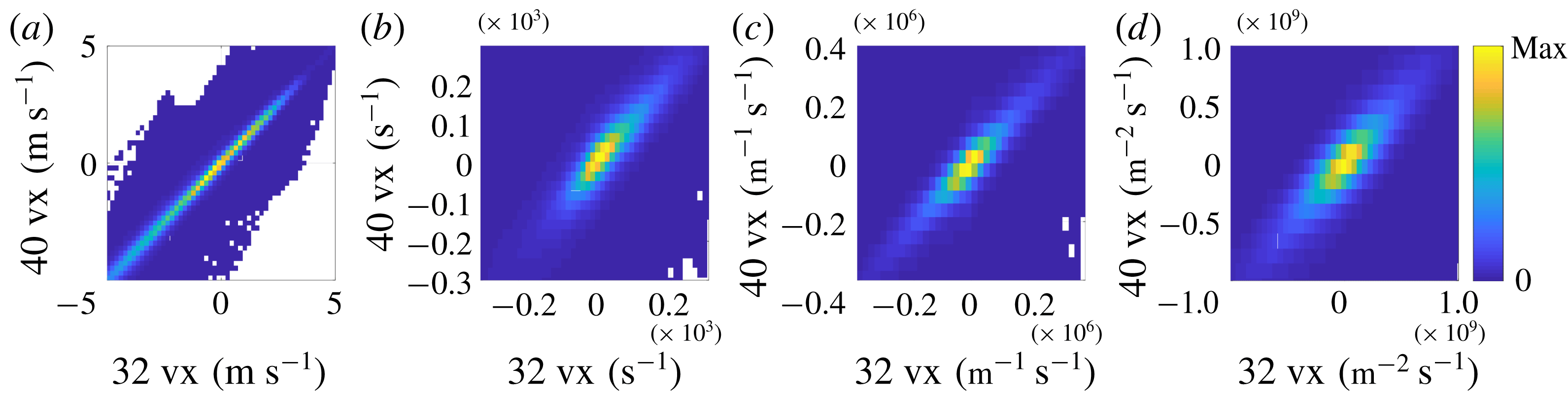
Joint probability density functions of (a)
 $u_{i}$
, (b)
 $\unicode[STIX]{x2202}u_{i}/\unicode[STIX]{x2202}x_{j}$
, (c)
 $\unicode[STIX]{x2202}^{2}u_{i}/\unicode[STIX]{x2202}x_{j}^{2}$
and (d)
 $\unicode[STIX]{x2202}^{3}u_{i}/\unicode[STIX]{x2202}x_{j}^{3}$
as computed using 32 vx and 40 vx grids for case 1.

Under-resolution results in a systematic reduction in the measured gradients, which is also affected by the numerical methods used for smoothing and gradient calculation. We assessed the impact of resolution by calculating vector fields using interrogation volume lengths ranging from 48 vx to 24 vx and comparing the results. We note that there was a large increase in measurement noise at interrogation boxes smaller than 32 vx. The issue of measurement noise in the cross-correlated velocity fields associated with interrogation box size is discussed in greater detail below.
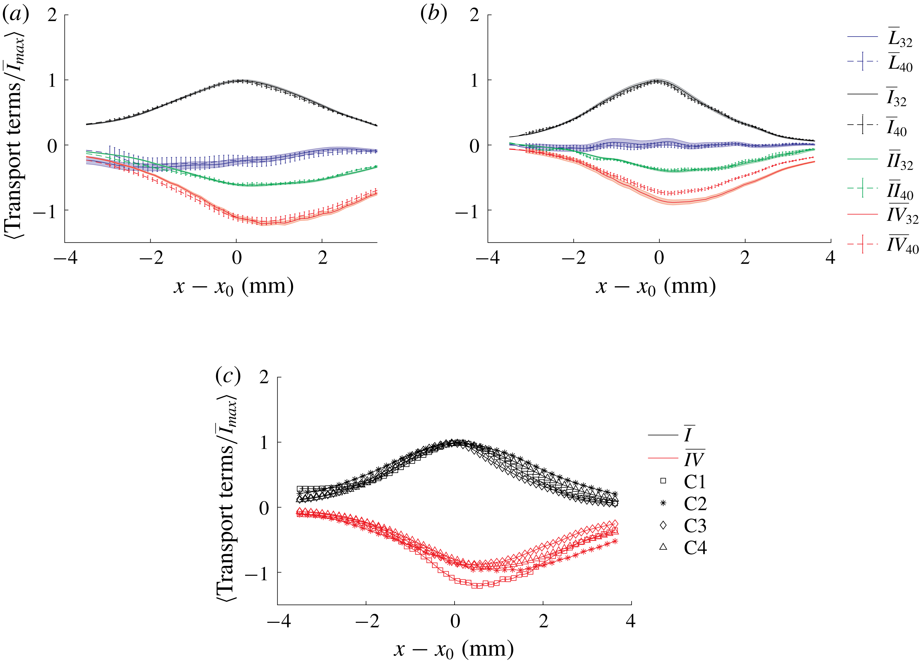
Figure 2 shows joint probability density functions of the velocity field and its gradients (up to third order) with interrogation boxes lengths of 40 vx and 32 vx for case 1. The higher-order derivatives were associated with higher noise, but there was no systematic under-prediction of the gradients at the lower resolution. Figure 3(a) shows the directly calculated terms in the average enstrophy transport budgets (
 $\overline{L}$
,
 $\overline{I}$
,
 $\overline{II}$
, and
 $\overline{IV}$
) for case 1 using the 40 vx and 32 vx interrogation boxes (the method by which
 $\unicode[STIX]{x1D707}$
and
 $\unicode[STIX]{x1D70C}$
were calculated to determine
 $\overline{IV}$
is discussed below). The results from both resolutions agree within the convergence uncertainty. We therefore conclude that the measurements were well-resolved in case 1.
Comparison of mean enstrophy transport terms demonstrating the degree of convergence with reducing interrogation box size in (a) case 1 and (b) case 3. Panel (c) shows the comparison between cases at 32 vx i. Shaded regions and the error bars represent the uncertainty in the mean due entirely to fluctuations (not systematic bias) for terms computed using 32 vx and 40 vx grids, respectively.

However, the same was not equally true for the more turbulent cases. Specifically, the measurements did not fully converge in the calculation of
 $\overline{IV}$
. This is demonstrated in figure 3(b), which shows
 $\overline{I}$
and
 $\overline{IV}$
calculated with 40 vx and 32 vx interrogation boxes for case 3. As can be seen,
 $\overline{I}$
did not change with the finer spatial resolution. However, the magnitude of
 $\overline{IV}$
increased with the finer resolution, indicating that the measurements were not fully resolved at 40 vx. As mentioned, it was not possible to further reduce the interrogation box due to noise issues, so it is not possible to determine whether the measurements were well-resolved at 32 vx. If not, this would result in a systematic under-estimation of the magnitude of
 $\overline{IV}$
and a corresponding under-estimation of
 $\overline{III}$
.
To estimate the bias uncertainty associated with possible under-estimation of
 $\overline{IV}$
, we speculate that, if fully resolved, the
 $\overline{I}$
and
 $\overline{IV}$
curves from the different cases should collapse when normalized by the maximum magnitude of
 $\overline{I}$
. Figure 3(c) shows
 $\overline{I}$
and
 $\overline{IV}$
from the different cases. Whereas the
 $\overline{I}$
curves collapse, the measured
 $\overline{IV}$
in case 1 has higher relative magnitude than in the other cases. Note that the collapse of
 $\overline{IV}$
for cases 2–4 does not indicate they are under-estimating by the same amount, as they are being normalized by the appropriate maximum
 $\overline{I}$
for each case.
Based on our assumption above, we estimate the bias uncertainty in the measurement of
 $\overline{IV}$
for cases 2–4 as the distance between the normalized
 $\overline{IV}$
curve for these cases and the
 $\overline{IV}$
curve for the fully resolved case 1, multiplied by the appropriate value of the maximum
 $\overline{I}$
for that case. The resultant asymmetric uncertainty bars are indicated in the figures in § 4.2.
While the resolution could potentially be increased by further decreasing the interrogation box size, this was limited by the need to have a sufficient number of particles in the interrogation box for accurate cross-correlation. A significant increase in random noise was observed when moving from 32 vx to 28 vx due to the reduced number of particles, and the particle seeding density could not be further increased due to unacceptable levels of ghost particles. Hence, an interrogation box length of 32 vx was selected for all further calculations.
3.3 Analysis of CH
$_{2}$
O PLIF

The
 $\text{CH}_{2}\text{O}$
measurements were used to estimate the instantaneous progress variable field
 $c$
in a plane corresponding to the centre of the T-PIV volume (
 $z=0$
). This allowed both estimation of the local fluid density and viscosity needed to calculate
 $IV$
in the reacting cases, as well as characterization of the enstrophy transport relative to the mean flame brush.
It is common practice to use PLIF to determine a progress-variable-like parameter based on the infinitely thin flame assumption. That is, the PLIF data are used to separate the flow into unburnt (
 $c=0$
) and burnt (
 $c=1$
) regions; intermediate values of
 $c$
are not considered. This is most commonly done based on OH PLIF images, in which the OH PLIF signal rapidly increases in the thin oxidation layer of the flame (Steinberg et al.
Reference Steinberg, Boxx, Arndt, Frank and Meier2011; Coriton, Steinberg & Frank Reference Coriton, Steinberg and Frank2014; Osborne et al.
Reference Osborne, Ramji, Carter, Peltier, Hammack, Lee and Steinberg2016, Reference Osborne, Ramji, Carter and Steinberg2017; Wabel, Skiba & Driscoll Reference Wabel, Skiba and Driscoll2017a
; Wabel et al.
Reference Wabel, Skiba, Temme and Driscoll2017b
).
However, using
 $\text{CH}_{2}\text{O}$
PLIF allows for a better estimation of the progress variable field. That is,
 $\text{CH}_{2}\text{O}$
occupies a region spanning the flame ‘preheat zone’ and is consumed by oxidation reactions. The region upstream of the
 $\text{CH}_{2}\text{O}$
therefore corresponds to
 $c\approx 0$
and the region downstream corresponds to
 $c\approx 1$
.
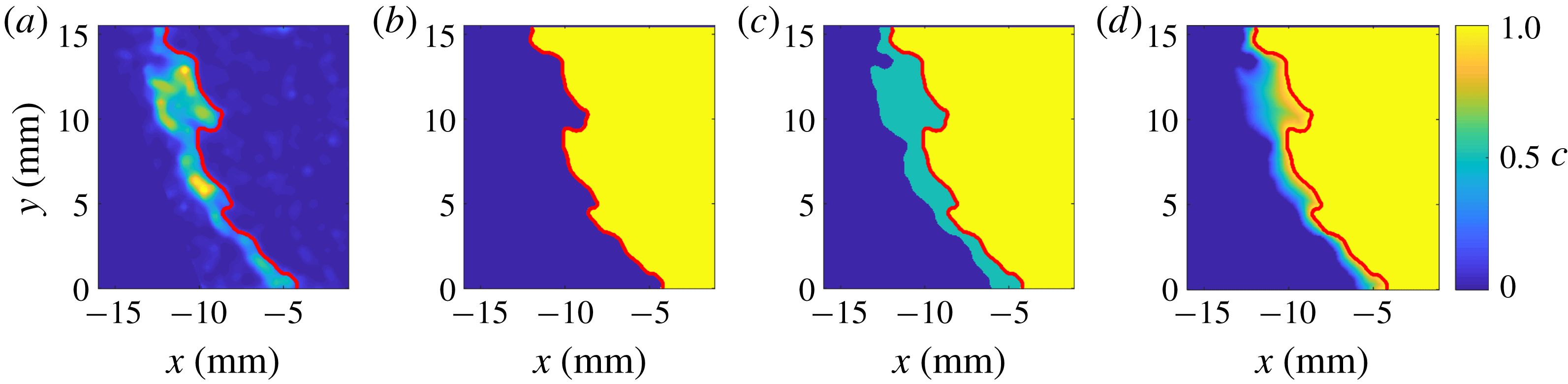
Instantaneous
 $\text{CH}_{2}\text{O}$
distribution (a) at case 4, and the associated
 $c$
fields as calculated via (b) infinitely thin flame assumptions, (c) an intermediate
 $c=0.5$
assumption and (d) linearly-interpolated relative distance assumption. The solid red curve demarcates the region containing
 $\text{CH}_{2}\text{O}$
from the inner recirculation zone.

We used three methods of deducing the intervening values of
 $c$
from the PLIF fields; these methods are demonstrated in figure 4. In the first, we assigned all locations upstream of the most downstream edge of the
 $\text{CH}_{2}\text{O}$
PLIF a value of
 $c=0$
. This is analogous to the infinitely thin flame method using OH PLIF. In the second, we assigned the region between the upstream and downstream edges a value of
 $c=0.5$
. In the third, we assigned the value of
 $c$
at any point in the
 $\text{CH}_{2}\text{O}$
region using a linear fit between
 $c=0$
and
 $c=1$
based on the distance of that point from the nearest upstream and downstream
 $\text{CH}_{2}\text{O}$
edges.
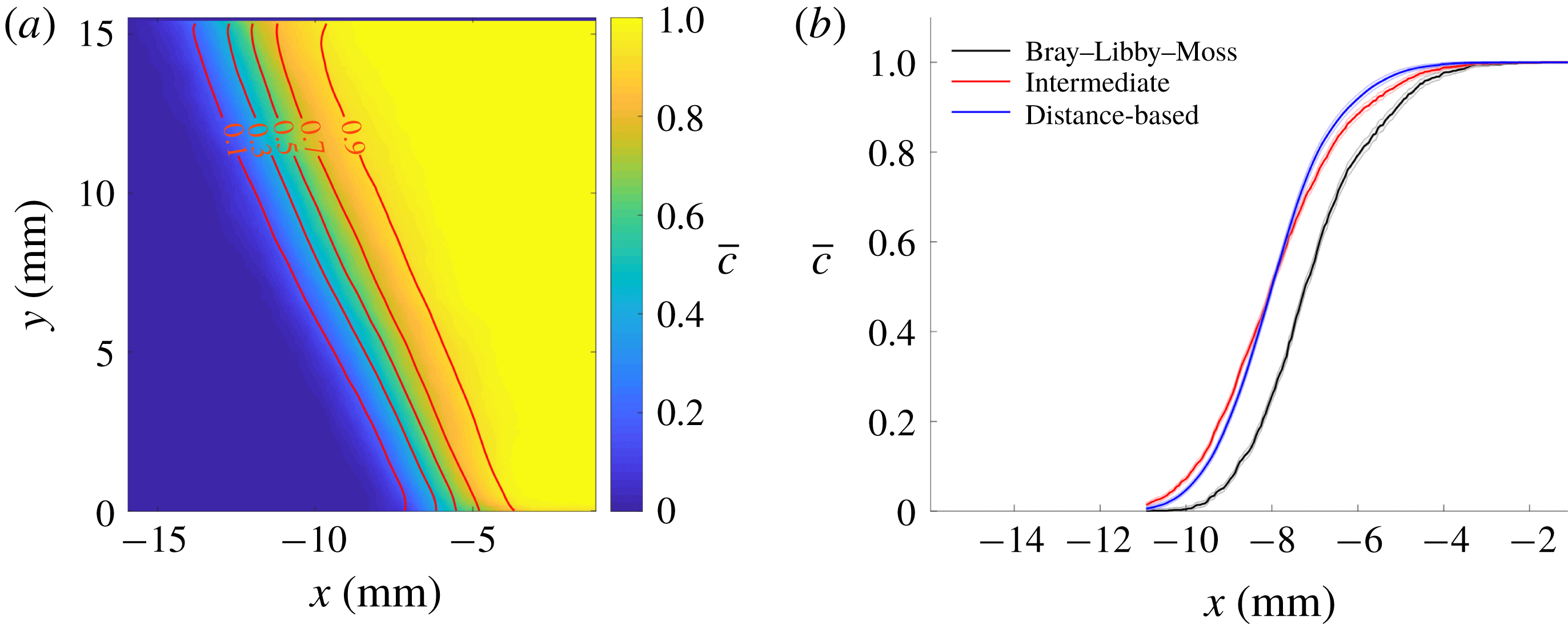
Ensemble averaging was performed to obtain the
 $\overline{c}$
field, which is shown in figure 5(a) based on the third method. Figure 5(b) shows typical
 $\bar{c}$
profiles through the mean flame brush using the three different methods. The infinitely thin flame assumption generated a
 $\overline{c}$
distribution that is shifted towards the products by approximately 1 mm relative to the other methods. The other two methods showed nearly identical results. The results presented below are based on the third (distance-based) method.
(a) Mean progress-variable field at case 4, calculated using the relative distance assumption; (b)
 $\overline{c}$
along
 $y=3~\text{mm}$
, as calculated using three estimation methods: infinitely thin flame (Bray, Libby & Moss Reference Bray, Libby and Moss1985; Libby Reference Libby1985), intermediate (
 $c\,=\,0.5$
where
 $\text{CH}_{2}\text{O}$
is present), and linear interpolation of
 $c$
between two edges of the
 $\text{CH}_{2}\text{O}$
region. Shaded region represents uncertainty in
 $\overline{c}$
.

We use the instantaneous
 $c$
field to estimate the values of
 $\unicode[STIX]{x1D707}$
and
 $\unicode[STIX]{x1D70C}$
needed for evaluation of
 $IV$
in the reacting cases. This is done by invoking a flamelet assumption across the instantaneous flame front. Dem et al. (Reference Dem, Stöhr, Arndt, Steinberg and Meier2014) performed Raman scattering measurements to determine the major species and temperature in the combustor used in the present study at conditions closely matching case 4 (the most turbulent case). They found that the thermo-chemical states – that is, the relationship between major species and temperature – within the inner shear layer corresponded closely to those of a laminar flame. For example, the measured instantaneous temperature at any given
 $\text{H}_{2}\text{O}$
mole fraction differed by less than 10 % from what would be expected in a laminar flame.
Hence, we assume that the instantaneous thermo-chemical state is a function of
 $c$
that can be determined from the corresponding laminar flame. The laminar flame profiles were determined using the same Cantera simulations used to determine
 $s_{L}^{0}$
and
 $\unicode[STIX]{x1D6FF}_{L}^{0}$
. Instantaneous
 $c$
fields were determined as described above, from which corresponding
 $\unicode[STIX]{x1D707}$
and
 $\unicode[STIX]{x1D70C}$
fields were determined. Since the PLIF data are taken with a higher resolution than the TPIV,
 $\unicode[STIX]{x1D707}$
and
 $\unicode[STIX]{x1D70C}$
were averaged in each interrogation box to determine the value corresponding to each vector. To test the impact of this calculation on the final results, the enstrophy transport budgets for case 4 were performed again, but using the second method described above for determining the instantaneous
 $c$
field (figure 4
c); the choice of
 $c$
field had negligible impact on the enstrophy transport budgets.
4 Results and discussion
4.1 Analysis of
$\overline{I}$
,
$\overline{II}$
and
$\left(\overline{III}+\overline{IV}\right)_{L}$


In this section, we consider the distributions of
 $\overline{I}$
,
 $\overline{II}$
and
 $\left(\overline{III}+\overline{IV}\right)_{L}$
in the reacting cases. We also compare the reacting
 $\left(\overline{III}+\overline{IV}\right)_{L}$
to
 $\overline{IV}_{L}$
in the non-reacting cases.
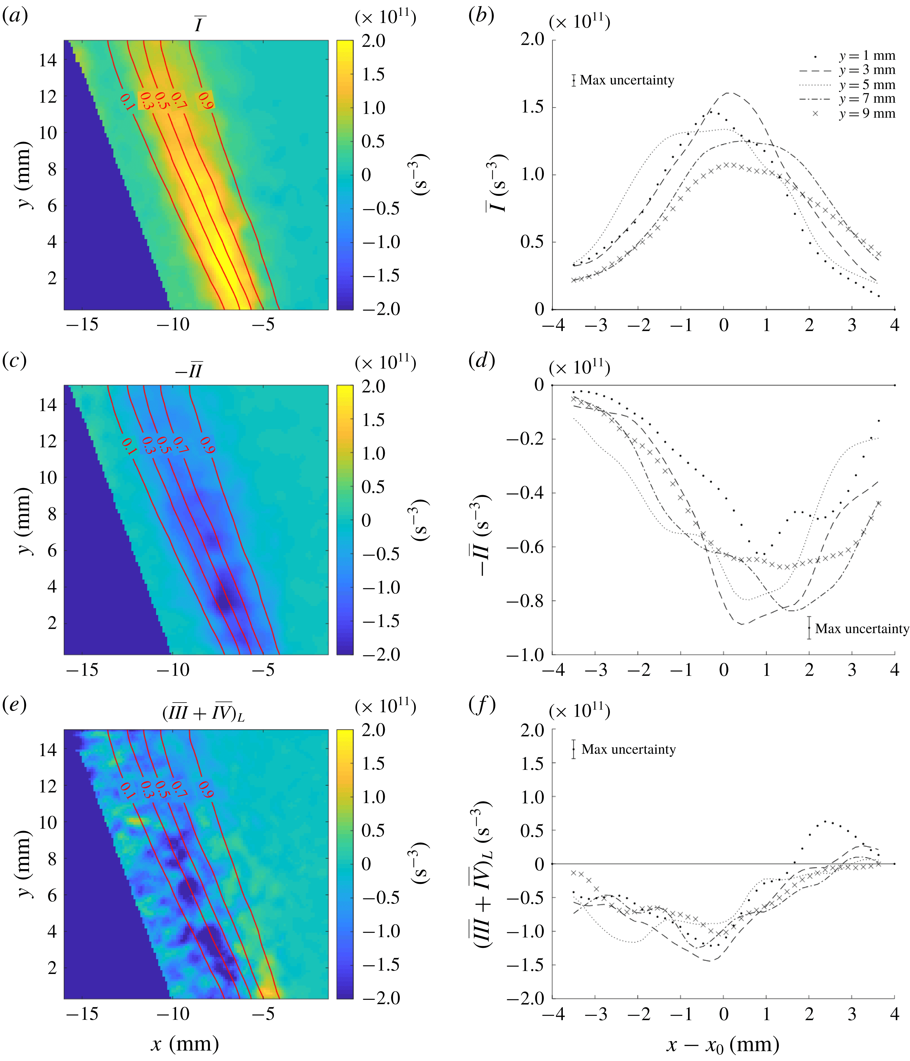
Figure 6 shows the
 $\overline{I}$
,
 $-\overline{II}$
and
 $(\overline{III}+\overline{IV})_{L}$
fields from case 2; these are overlaid by contours of
 $\bar{c}$
indicating the position of the flame brush. Also shown are profiles of these terms along the
 $x$
-direction at several downstream locations
 $y$
. As expected, the production and dilatation terms are strictly positive and negative, respectively. In contrast,
 $(\overline{III}+\overline{IV})_{L}$
is negative towards the reactants, but obtains slightly positive values towards the products. A preliminary comparison of
 $\overline{IV}$
in figure 3(c) to
 $(\overline{III}+\overline{IV})_{L}$
shows that the maximum magnitude of the latter occurs further towards the reactants and the magnitude drops more steeply towards the products. These observations indicate that the baroclinic torque acts as a source of enstrophy towards the product side of the flame brush.
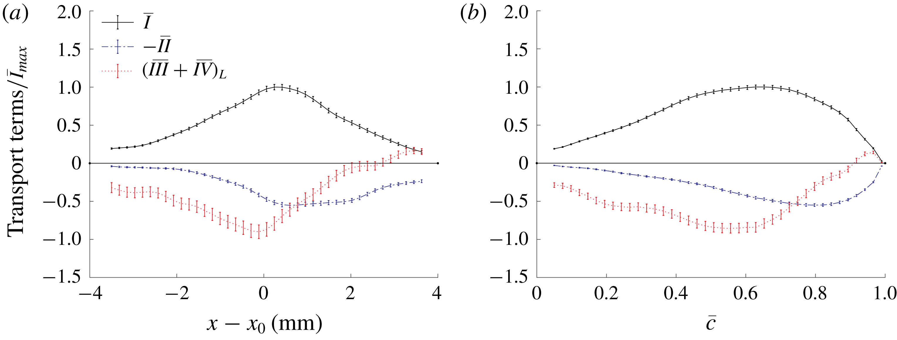
It is common practice in DNS of flames in HIT to plot budgets versus the mean progress variable, as opposed to spatial coordinates. However, as seen in figure 6, the budgets are not necessarily well-described by the position in the
 $\overline{c}$
field in this inhomogeneous system. For reference, figure 7 shows profiles of
 $\overline{I}$
,
 $-\overline{II}$
,
 $(\overline{III}+\overline{IV})_{L}$
at
 $y=3$
mm for case 2, all normalized by the maximum value of
 $\overline{I}$
, versus both physical space and mean progress variable. The trends are qualitatively similar, but the profiles are skewed towards the products in
 $\overline{c}$
space compared to physical space. The analysis below will be presented in physical space; the mean transport budgets also are presented as function of
 $\overline{c}$
for reference in appendix A.
Reynolds-averaged enstrophy transport terms:
 $\overline{I}$
,
 $-\overline{II}$
and
 $(\overline{III}+\overline{IV})_{L}$
for case 2 on the central plane of the T-PIV volume (
 $z=0~\text{mm}$
). Contour lines of the
 $\overline{c}$
field are overlaid with enstrophy budget plots. The region containing the outer recirculation zone is masked because this area was not seeded for the T-PIV measurements. Radial
 $x$
profiles at various downstream locations
 $y$
for each term are shown to the right. Reference
 $x_{0}$
is the axial coordinate of maximum vortex stretching
 $\overline{I}_{max}$
at each
 $y$
.

The flame is stabilized in the inner shear layer between the inflowing reactants and the inner recirculation zone, resulting in a spatial overlap of the flame brush with the regions of high enstrophy production due to vortex stretching. The maximum enstrophy production due to vortex stretching occurs 3 mm above the exit plane and decreases further downstream due to weakening of the shear layer.
The mean dilatation acts to dissipate enstrophy across the flame (
 $-\overline{II}<0$
) and is therefore confined to the regions within the flame brush. A fluid element passing through the flame undergoes a change in volume by a factor of approximately five. Thus, the length scale of any vortical structures passing through the flame is correspondingly increased, attenuating vorticity. Unlike
 $\overline{I}$
, dilatation remains similar in magnitude – within measurement uncertainty – across a range of axial locations due to the fixed expansion across the flame.
The residual term
 $(\overline{III}+\overline{IV})_{L}$
, represents the cumulative effect of baroclinic torque and viscous dissipation/diffusion on the enstrophy transport. Note that, while dissipation is strictly negative, the diffusion may be of either sign. Holzner et al. (Reference Holzner, Liberzon, Nikitin, Luthi, Kinzelbach and Tsinober2008) and Watanabe et al. (Reference Watanabe, Sakai, Nagata, Ito and Hayase2014) observed that viscous diffusion of enstrophy had a positive contribution to enstrophy transport across the turbulent/non-turbulent boundary, while dissipation remained strictly negative. However, the relative magnitude of dissipation is usually greater than that of diffusion;
 $\overline{IV}$
was strictly negative in all cases studied here.
Normalized enstrophy budget terms for case 2 at
 $y=3~\text{mm}$
. (a) Versus radial position
 $x-x_{0}$
. (b) Versus mean progress variable
 $\bar{c}$
. The error bars represent the convergence uncertainty in the mean.

Comparison of normalized
 $(\overline{III}+\overline{IV})_{L}$
(solid red) in a reacting flow to normalized
 $\overline{IV}_{L}$
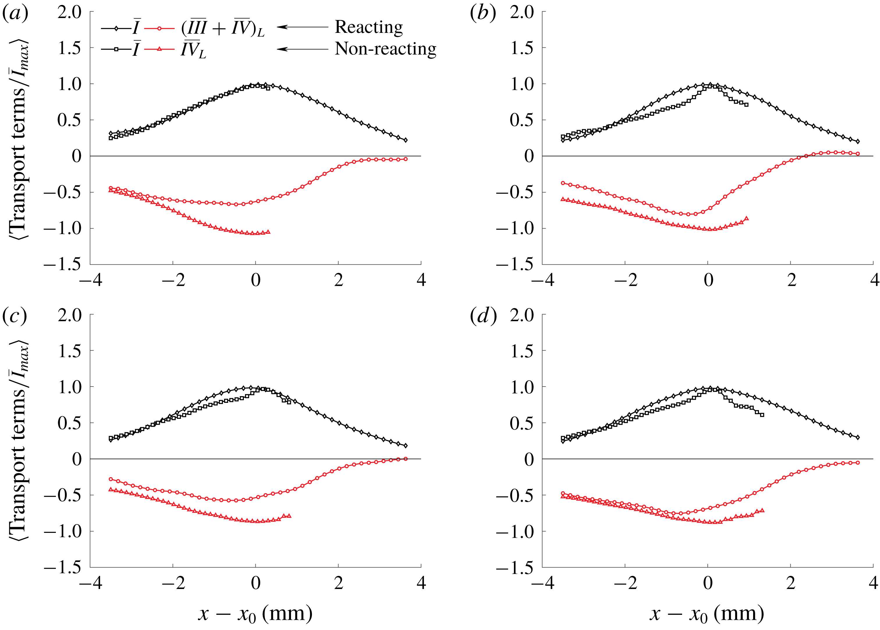
(dashed red) in a non-reacting flow in (a) case 1, (b) case 2, (c) case 3, (d) case 4. Vortex stretching in a reacting flow (solid black) is compared to vortex stretching in non-reacting flow (dashed black). The non-reacting flow profile was limited by the field of view.

As a first assessment of the impact of baroclinic torque, figure 8 compares the profiles of
 $(\overline{III}+\overline{IV})_{L}$
in the reacting cases to
 $\overline{IV}_{L}$
in the non-reacting cases. It would be expected that the reacting cases would exhibit greater dissipation in the products (i.e. at higher
 $x$
) due to the increase in temperature and viscosity. However,
 $(\overline{III}+\overline{IV})_{L}$
in the reacting cases was greater than
 $\overline{IV}_{L}$
in the non-reacting cases. This is indicative of a positive mean baroclinic torque that is a source of enstrophy.
4.2 Baroclinic torque
We now aim to isolate the effects of baroclinic torque from dissipation, i.e. estimate
 $\overline{III}_{L}$
based on the measured data. The approach described in § 3.2 was used to approximate the magnitude of
 $\overline{IV}$
and its uncertainty.
Reynolds-averaged
 $\overline{IV}$
and
 $\overline{III}_{L}$
for case 2 on the central plane of the T-PIV volume (
 $z=0~\text{mm}$
). Contour lines of the
 $\overline{c}$
field are overlaid with enstrophy budget plots. Corresponding radial
 $x$
profiles at various downstream locations
 $y$
are shown to the right.

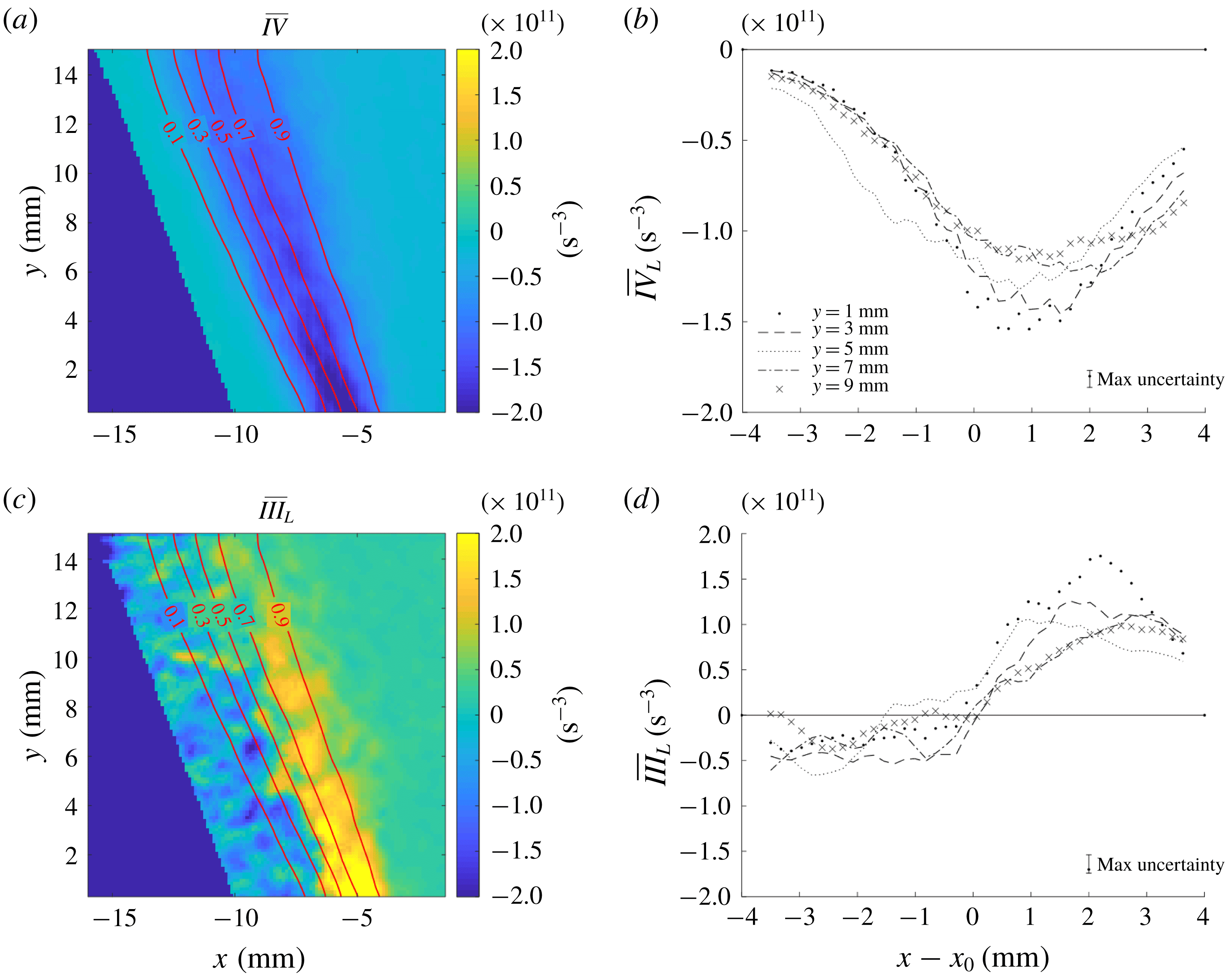
Figure 9 shows the
 $\overline{III}_{L}$
and
 $\overline{IV}$
fields on the central plane of TPIV volume in case 2; radial profiles along select
 $y$
locations also are shown. Viscous dissipation is a sink of enstrophy (
 $\overline{IV}<0$
) within the shear layer. The maximum value of
 $\overline{IV}$
decreases with
 $y$
in a similar manner to
 $\overline{I}$
shown in figure 6. This trend was also observed at the higher turbulence intensities. Such a balance was also found to naturally hold for non-reacting HIT and HIT at high turbulence intensities by Bobbitt et al. (Reference Bobbitt, Lapointe and Blanquart2016).
The baroclinic torque
 $\overline{III}_{L}$
obtains small negative values on the reactant side of the flame brush and considerably larger positive values on the product side. This qualitatively agrees with the attenuation of reactant side vorticity and generation of product side vorticity seen in laminar flame/vortex interactions (Louch & Bray Reference Louch and Bray1998; Mueller et al.
Reference Mueller, Driscoll, Reuss, Drake and Rosalik1998). However, in these interactions, the vorticity attenuation generally was greater than or comparable to the vorticity production. Here, we observe relatively weak attenuation and much stronger generation.
The sign of baroclinicity may be interpreted in terms of the alignment between density and pressure gradients. Density gradients are perpendicular to the local flame front, whereas the pressure gradients are determined by the simultaneous action of the turbulent vortices, combustor scale swirling flow and flame. The data demonstrate that the orientation and magnitude of the pressure field associated with the swirling flow results in significant baroclinic enstrophy production relative to what would occur in a non-swirling flow. Note that this indicates that the significance of baroclinic enstrophy production does not have a universal relationship with the turbulence and flame properties, but depends on the pressure field associated with the particular configuration of interest.
Normalized radial profiles of the decoupled enstrophy transport terms in (a) case 1, (b) case 2, (c) case 3, (d) case 4. All radial profiles averaged over downstream locations
 $y$
.

The transition from
 $\overline{III}_{L}<0$
to
 $\overline{III}_{L}>0$
occurs around the location of maximum vortex stretching (i.e.
 $x=x_{0}$
) at all downstream positions. The decreasing strength of the radial pressure gradient with axial distance results in a corresponding decrease in the peak magnitude of the baroclinic torque. Nevertheless, the significance of enstrophy production by baroclinic torque remains comparable to that of vortex stretching and dissipation, both of which also decrease with axial distance.
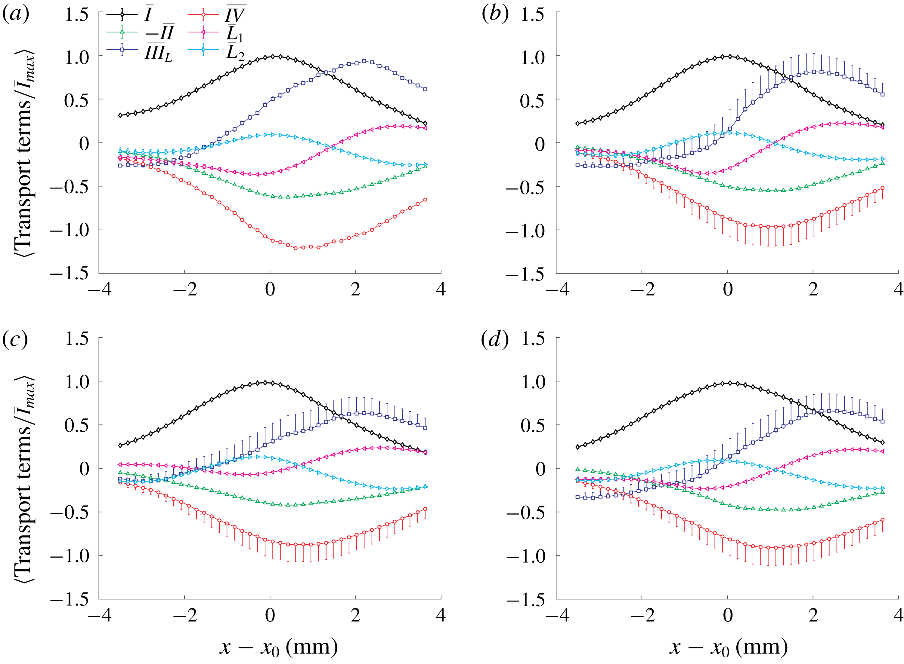
The radial profiles of
 $\langle \overline{III}_{L}\rangle$
and
 $\langle \overline{IV}\rangle$
(averaged over axial locations) are shown in figure 10 for the different cases. The uncertainties in
 $\overline{I}$
and
 $-\overline{II}$
are due to statistical convergence. The asymmetric uncertainty bars in
 $\langle \overline{III}_{L}\rangle$
and
 $\langle \overline{IV}\rangle$
combine the systematic under-prediction of
 $\overline{IV}$
and the convergence uncertainty. The systematic bias results in an under-estimation of the magnitude of
 $\langle \overline{IV}\rangle$
and a corresponding under-estimation of
 $\langle \overline{III}_{L}\rangle$
.
Also shown in figure 10 are normalized radial profiles of the advection of enstrophy by the mean flow (
 $\overline{L}_{1}$
) and the mean turbulent transport (
 $\overline{L}_{2}$
), which together constitute the Lagrangian derivative, viz.
 $$\begin{eqnarray}\overline{L}=\underbrace{\overline{u}_{i}\frac{\unicode[STIX]{x2202}\overline{\unicode[STIX]{x1D6FA}}}{\unicode[STIX]{x2202}x_{j}}}_{\overline{L}_{1}}+\underbrace{\overline{u_{i}^{\prime }\frac{\unicode[STIX]{x2202}\unicode[STIX]{x1D6FA}^{\prime }}{\unicode[STIX]{x2202}x_{j}}}}_{\overline{L}_{2}}.\end{eqnarray}$$
Here,
 $u_{i}^{\prime }$
and
 $\unicode[STIX]{x1D6FA}^{\prime }$
represent the fluctuating components of velocity and enstrophy, respectively. Figure 10 shows that
 $\overline{L}_{2}$
is the main contributor to
 $\overline{L}$
inside the shear layer, whereas
 $\overline{L}_{1}$
is the main contributor inside the central recirculation zone. However, the relative magnitude of
 $\overline{L}_{1}$
and
 $\overline{L}_{2}$
to terms
 $\overline{I}$
through
 $\overline{IV}$
is small.
For all test cases, the baroclinic torque attenuates enstrophy at the earlier stages of combustion, but results in significant enstrophy production on the product side of the flame brush. Indeed, the baroclinic torque is the largest source of enstrophy at positions farthest towards the products, viz.
 $x-x_{0}\gtrsim 2~\text{mm}$
. Moreover, the baroclinic torque remains significant relative to the other terms in the enstrophy transport equation across cases; there is little difference in the ratio of baroclinic torque to vortex stretching across cases once the uncertainty is considered. This observation also is true for the budgets as a function of
 $\bar{c}$
shown in appendix A.
5 Conclusions
This study quantified the mechanisms contributing to Reynolds-averaged enstrophy transport in turbulent swirl flames using high-resolution T-PIV and
 $\text{CH}_{2}\text{O}$
PLIF measurements. The main conclusions are that (i) baroclinic torque is a significant source of enstrophy production relative to the effects of vortex stretching, viscous dissipation and dilatation; and (ii) the relative significance of barloclinic torque remains high with increasing turbulence intensity over the range of conditions studied. The former indicates that flame-induced turbulence production should be considered when modelling swirl combustion. The latter contrasts with DNS of flames in HIT, indicating that caution must be applied when extending results from such a canonical configuration to more practical systems. Indeed, the results indicate that the significance of baroclinic enstrophy production is not solely determined by the flame and turbulence properties, but is strongly influenced by the pressure field associated with the configuration being studied.
Future work should (i) extend this analysis to higher turbulence intensities, which will require the development of higher resolution 3-D velocimetry techniques; (ii) analyse the inter-scale energy transfer in such swirl flames to determine how the turbulence associated with flame-generated enstrophy impacts the energy dynamics; and (iii) perform DNS of similar swirl flames to obtain insights not available from experimental data.
Acknowledgements
This work was supported by the US Air Force Office of Scientific Research under grant FA9550-17-0011, Project Monitor Dr Chiping Li.
Appendix A
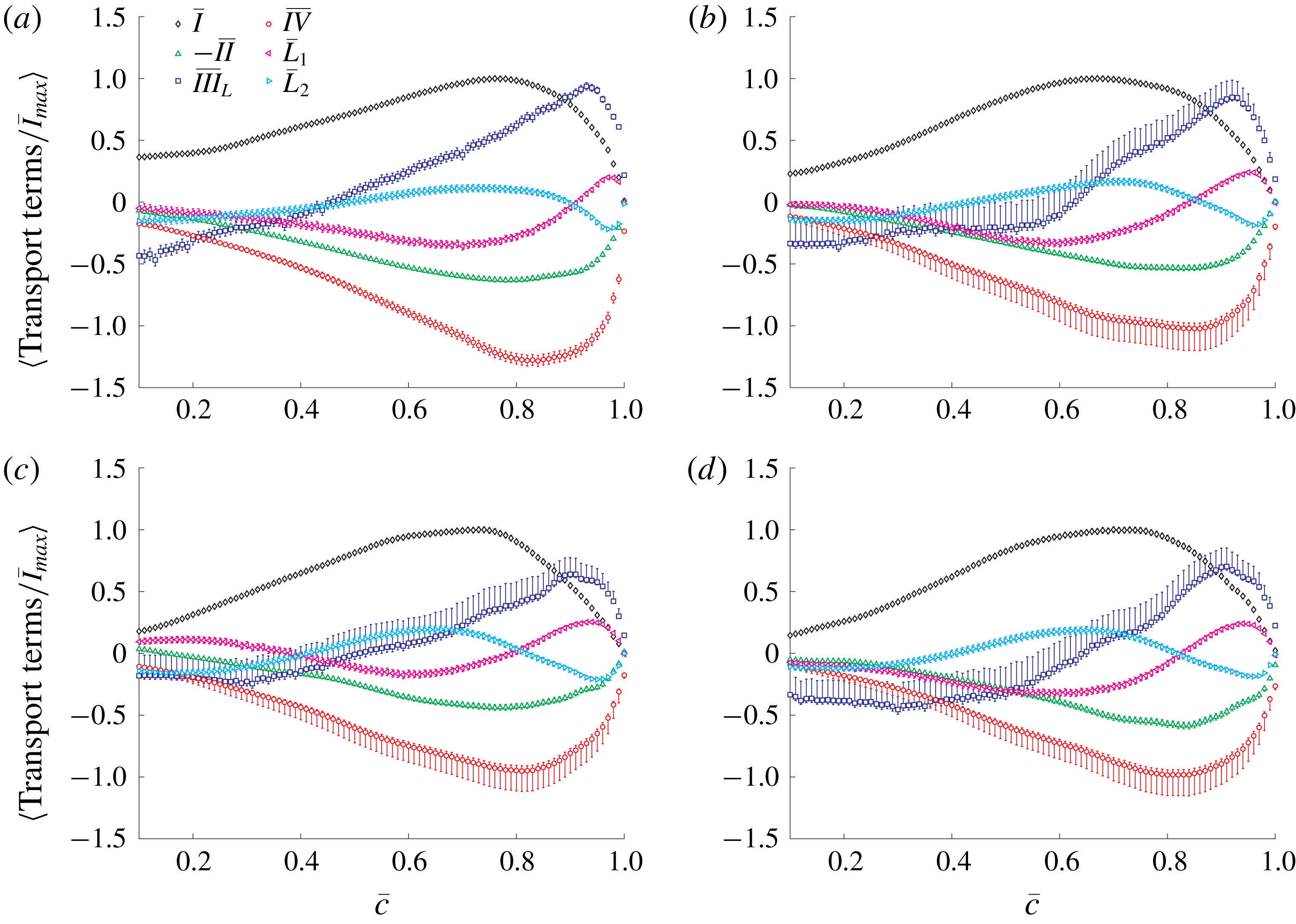
For completeness, figure 11 shows the mean enstrophy transport budgets conditioned on the mean reaction progress variable
 $\overline{c}$
. The trends and conclusions are the same as figure 10.
Normalized enstrophy transport terms conditioned on the mean progress variable in (a) case 1, (b) case 2, (c) case 3, (d) case 4.