2 Model

2.1 Two-scale dynamics

If a turbine array spans only part of the flow cross-section, two principal scales of flow phenomena may be assumed: smaller features at the scale of the turbine width and larger features at the scale of the array width. The additional assumption that array-scale flow phenomena take place much more slowly and over much greater distances than local-scale flow phenomena allows the two sets of events to be separated and analysed quasi-independently (Nishino & Willden Reference Nishino and Willden2012b ; Vogel et al. Reference Vogel, Houlsby and Willden2016). This concept of scale separation redefines the global blockage, $B_{G}$ , as the product of an array blockage, $B_{A}$ , which represents the ratio of the cross-sectional area of the array to that of the channel, and a local blockage, $B_{L}$ , which represents the ratio of the cross-sectional area of the turbine to that of its local flow passage, thus giving

(2.1a-c ) $$\begin{eqnarray}B_{G}=\frac{nA_{T}}{hw_{C}},\quad B_{A}=\frac{hw_{A}}{hw_{C}}\quad \text{and}\quad B_{L}=\frac{A_{T}}{hw_{L}},\end{eqnarray}$$

in which $n$ is the number of identical and equally spaced turbines; $A_{T}$ is the turbine swept area; $h$ is the fluid depth; $w_{C}$ and $w_{A}$ are the widths of the channel and array; and $w_{L}(=w_{A}/n)$ is the width of the local flow passage. This revised definition allows consideration of different turbine arrangements, with each arrangement of a given $B_{G}$ defined by two parameters: the relative width of the array, $B_{A}$ , and the relative size of the turbines within it, $B_{L}$ (Nishino & Willden Reference Nishino and Willden2012b ; Vogel et al. Reference Vogel, Houlsby and Willden2016).

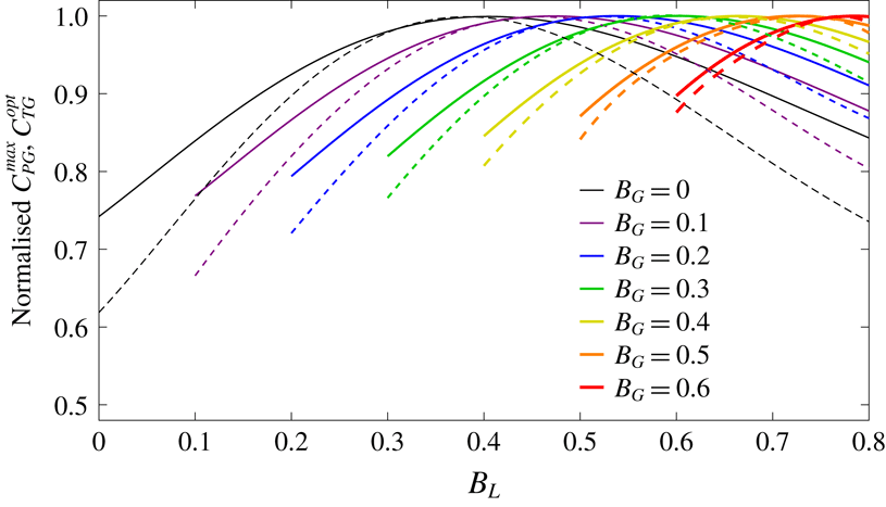
Results from the two-scale actuator disc model of Nishino & Willden (Reference Nishino and Willden2012b ) show that for each arrangement of a given $B_{G}$ , there is an optimal turbine resistance: that is to say, there is an optimal global thrust coefficient, $C_{TG}^{opt}$ , which produces a maximum global power coefficient, $C_{PG}^{max}$ . The prefix ‘global’ is used to indicate that these parameters represent the normalisation of array thrust and power with respect to the large-scale flow: $C_{TG}$ is defined as the ratio of applied thrust, $T$ , to the integral of channel-scale dynamic pressure, $0.5\unicode[STIX]{x1D70C}u_{C}^{2}$ (in which $\unicode[STIX]{x1D70C}$ is the fluid density and $u_{C}$ is the channel-scale velocity), over the swept area of the array, $A_{A}(=nA_{T})$ , whereas $C_{PG}$ is defined as the ratio of available power, $P_{av}$ , to the kinetic energy flux of the channel-scale flow passing through an equivalent area, $0.5\unicode[STIX]{x1D70C}A_{A}u_{C}^{3}$ . The optimal turbine resistance is determined by the balance between the local-scale slowing of flow that accompanies energy extraction and the array-scale choking of flow which ultimately limits the amount of power that can be produced.

Figure 1.

Results from the two-scale actuator disc model of Nishino & Willden (Reference Nishino and Willden2012b ): variations in maximum global power coefficient $C_{PG}^{max}$ (solid lines) and corresponding optimal global thrust coefficient $C_{TG}^{opt}$ (dashed lines) with local blockage $B_{L}$ for a range of global blockages $B_{G}$ , normalised by the respective maxima for each $B_{G}$ .

Furthermore, for each $B_{G}$ there is an optimal turbine arrangement which produces a peak $C_{PG}^{max}$ . This optimal arrangement is determined by a similar balance between the same detrimental array-scale choking effect and a beneficial local blockage effect. As $B_{L}$ is increased from $B_{G}$ (and $B_{A}$ is reduced such that $B_{G}=B_{A}B_{L}$ remains constant), $C_{PG}^{max}$ initially increases as the decreasing potential for flow to divert between the turbines enables higher optimal turbine resistances. As $B_{L}$ is further increased, however, $C_{PG}^{max}$ then begins to reduce as the increasing potential for flow to divert around the array necessitates lower optimal turbine resistances. The optimal local blockage is thus essentially the arrangement that makes it most difficult for flow to pass around the turbines: more specifically, it is the arrangement for which this local blockage effect enables the production of a peak power coefficient through the application of a near-peak thrust coefficient (figure 1). (A differing dependence on velocity ensures that the peak $C_{PG}^{max}$ and $C_{TG}^{opt}$ do not coincide exactly.) It seems intuitive, then, that the optimal local blockage must depend on the balance of forces driving and resisting the channel-scale flow, the effects of which are not captured by this two-scale actuator disc model.

To explore this dependence, a more comprehensive theoretical model must be developed in order to describe the effects of local blockage on the performance of tidal turbines operating in more realistic channel flow conditions. As a first step towards the development of such a model, the present study uses numerical simulations to provide new insight into the effects of channel-scale dynamics on the optimal turbine arrangement and potential for enhanced power capture.

2.2 Combined array and channel model

A numerical model is used to explore the potential for local blockage effects to enhance the performance of tidal turbines operating in rough and oscillatory channel flow. This model uses the depth-averaged shallow water equations to simulate head-driven flow through an idealised channel, and a sub-grid-scale actuator disc model to represent a single cross-stream row of turbines as a line sink of fluid momentum. Whereas the idealised analytical approach of Garrett & Cummins (Reference Garrett and Cummins2013) enabled the exploration of a broad parameter space, the more detailed numerical approach adopted herein necessitates a focus on a more specific set of flow conditions. Accordingly, the simulations have been designed with a view to capturing the range of conditions observed at the majority of candidate tidal energy sites. In addition to the local blockage and local resistance of the turbines, the key variables considered are the width of the array; the level of background roughness; the frequency of the tidal forcing; and the amplitude of the current velocity. Fixed variables, in this case, include the length, width and still water depth of the channel; the global blockage of the array; the number of turbine rows; and the value of the horizontal eddy viscosity coefficient. The use of a two-dimensional model naturally requires a degree of abstraction, but realistic values are sought to ensure that the results reflect, insofar as possible, the flow conditions in actual tidal channels.

The discontinuous Galerkin (DG) version of the open-source hydrodynamic model ADCIRC (Kubatko, Westerink & Dawson Reference Kubatko, Westerink and Dawson2006; Kubatko et al. Reference Kubatko, Bunya, Dawson and Westerink2009) is used to simulate uniform, depth-averaged flow through a channel of length, $l_{C}=20~\text{km}$ ; width, $w_{C}=4~\text{km}$ ; and still water depth, $h_{sC}=20~\text{m}$ (figure 2). The numerical code, which is described in greater detail by Serhadlıoğlu (Reference Serhadlıoğlu2014), solves the two-dimensional shallow water equations, which are presented herein as

(2.2) $$\begin{eqnarray}\frac{\unicode[STIX]{x2202}\unicode[STIX]{x1D702}}{\unicode[STIX]{x2202}t}+\frac{\unicode[STIX]{x2202}uh}{\unicode[STIX]{x2202}x}+\frac{\unicode[STIX]{x2202}vh}{\unicode[STIX]{x2202}y}=0,\end{eqnarray}$$

(2.3) $$\begin{eqnarray}\displaystyle & & \displaystyle \frac{\unicode[STIX]{x2202}uh}{\unicode[STIX]{x2202}t}+\frac{\unicode[STIX]{x2202}}{\unicode[STIX]{x2202}x}\bigg[u^{2}h+\frac{g(h^{2}-h_{s}^{2})}{2}\bigg]+\frac{\unicode[STIX]{x2202}uvh}{\unicode[STIX]{x2202}y}=g\unicode[STIX]{x1D702}\frac{\unicode[STIX]{x2202}h_{s}}{\unicode[STIX]{x2202}x}\nonumber\\ \displaystyle & & \displaystyle \qquad -\,C_{d}u\sqrt{u^{2}+v^{2}}+\unicode[STIX]{x1D708}\bigg[2\frac{\unicode[STIX]{x2202}^{2}uh}{\unicode[STIX]{x2202}x^{2}}+\frac{\unicode[STIX]{x2202}^{2}uh}{\unicode[STIX]{x2202}y^{2}}+\frac{\unicode[STIX]{x2202}^{2}vh}{\unicode[STIX]{x2202}x\unicode[STIX]{x2202}y}\bigg]\end{eqnarray}$$

and

(2.4) $$\begin{eqnarray}\displaystyle & & \displaystyle \frac{\unicode[STIX]{x2202}vh}{\unicode[STIX]{x2202}t}+\frac{\unicode[STIX]{x2202}uvh}{\unicode[STIX]{x2202}x}+\frac{\unicode[STIX]{x2202}}{\unicode[STIX]{x2202}y}\bigg[v^{2}h+\frac{g(h^{2}-h_{s}^{2})}{2}\bigg]=g\unicode[STIX]{x1D702}\frac{\unicode[STIX]{x2202}h_{s}}{\unicode[STIX]{x2202}y}\hspace{42.67912pt}\nonumber\\ \displaystyle & & \displaystyle \qquad -\,C_{d}v\sqrt{u^{2}+v^{2}}+\unicode[STIX]{x1D708}\bigg[\frac{\unicode[STIX]{x2202}^{2}vh}{\unicode[STIX]{x2202}x^{2}}+2\frac{\unicode[STIX]{x2202}^{2}vh}{\unicode[STIX]{x2202}y^{2}}+\frac{\unicode[STIX]{x2202}^{2}uh}{\unicode[STIX]{x2202}x\unicode[STIX]{x2202}y}\bigg],\end{eqnarray}$$

in which $\unicode[STIX]{x1D702}$ is the elevation of the free surface above the still water level; $h_{s}$ is the still water depth; $h$ ( $=h_{s}+\unicode[STIX]{x1D702}$ ) is the total depth; $u$ and $v$ are the streamwise ( $x$ -directed) and cross-stream ( $y$ -directed) components of the depth-averaged velocity vector $\boldsymbol{u}$ ; $g$ is acceleration due to gravity; $C_{d}$ is the dimensionless seabed drag coefficient; and $\unicode[STIX]{x1D708}$ is the horizontal eddy viscosity coefficient. Implicit in the presentation of these equations are the assumptions of a fixed seabed (i.e. no erosion or sedimentation); a spatially and temporally constant horizontal eddy viscosity coefficient; negligible Coriolis forcing; and a flow which is driven solely by a gradient in free surface elevation and which loses energy, in the absence of turbines, through quadratic seabed drag, changes in cross-section and turbulent mixing. Tangential slip conditions are specified for the channel walls and flow is driven by establishing a head difference between two Dirichlet boundaries, which are placed in much deeper water (at still water depths of 1 km) and far beyond the ends of the central channel (at distances of 50 km) so as to minimise the reflection of error waves through the domain of interest.

Figure 2.

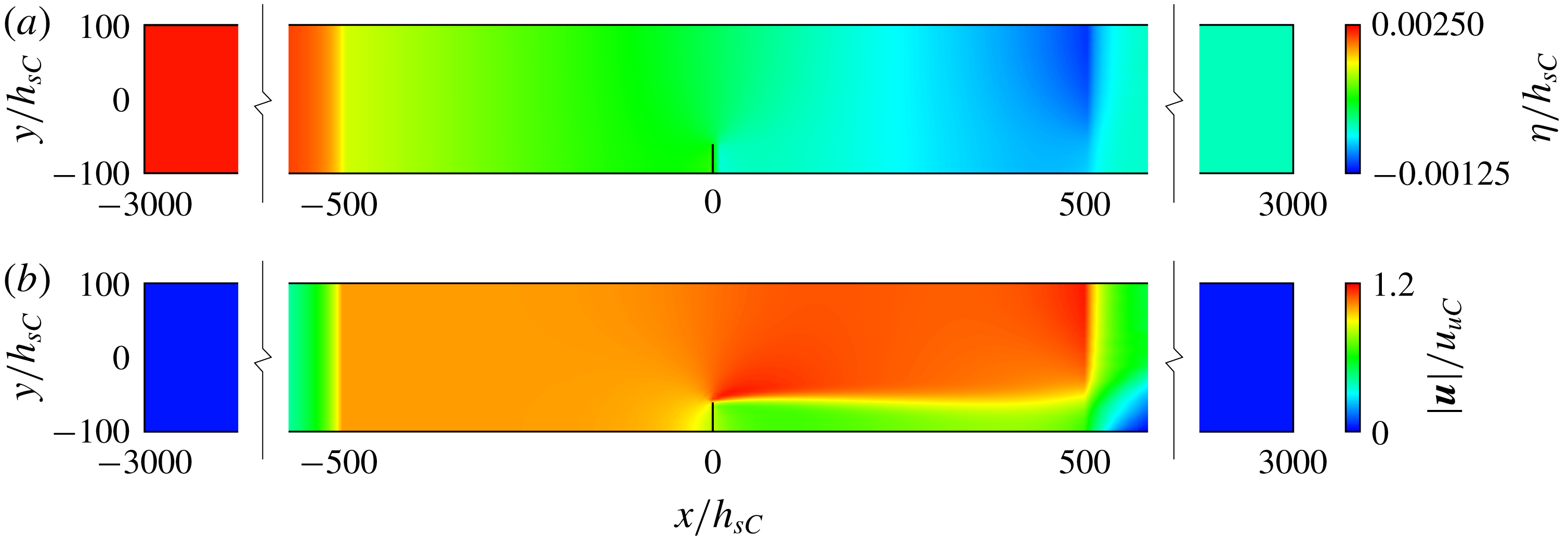
Plan views of the idealised channel ( $-500\leqslant x/h_{sC}\leqslant 500$ ) and greater model domains with (near-)steady-state contours of: (a) free surface elevation $\unicode[STIX]{x1D702}(x,y)$ , normalised by channel still water depth $h_{sC}$ , and (b) magnitude of the corresponding depth-averaged velocity $\boldsymbol{u}(x,y)$ , normalised by unexploited streamwise channel velocity $u_{uC}$ . Steady and oscillatory currents are produced by controlling the water levels at $x/h_{sC}=-3000$ and $3000$ , and the position of the turbine array is marked by the black vertical line at $x/h_{sC}=0$ . Adapted from Bonar et al. (Reference Bonar, Adcock, Venugopal and Borthwick2018).

For the less well-defined model parameters, empirical formulae are used to obtain representative values. The seabed drag coefficient is calculated, following Soulsby (Reference Soulsby1997), as $C_{d}=[\unicode[STIX]{x1D705}/(\unicode[STIX]{x1D6FE}+\text{ln}(z_{0}/h))]^{2}$ , in which $\unicode[STIX]{x1D705}$ is the dimensionless von Kármán constant, $\unicode[STIX]{x1D6FE}$ is an additional dimensionless coefficient and $z_{0}$ is a characteristic roughness length. A value of $C_{d}$ of 0.0025 would be typical for a shallow water model such as this, but herein a range of $z_{0}$ is used, taking $\unicode[STIX]{x1D705}=0.4$ and $\unicode[STIX]{x1D6FE}=1$ (as for a velocity profile which is logarithmic throughout the water column) and $h=20~\text{m}$ , to obtain representative values for a variety of seabed materials: from fine silt ( $z_{0}\approx 0.02~\text{mm}$ ; $C_{d}\approx 0.001$ ) to coarse gravel ( $z_{0}\approx 5~\text{mm}$ ; $C_{d}\approx 0.003$ ), and including both artificially smooth ( $z_{0}\approx 0.0001~\text{mm}$ ; $C_{d}\approx 0.0005$ ) and exceedingly rough ( $z_{0}\approx 25~\text{mm}$ ; $C_{d}\approx 0.005$ ) surfaces. The value of the horizontal eddy viscosity coefficient is then calculated, following Borthwick & Barber (Reference Borthwick and Barber1992), as $\unicode[STIX]{x1D708}=5.9h|\boldsymbol{u}|\sqrt{C_{d}}$ , which, taking $h=20~\text{m}$ , $C_{d}=0.0005$ and $|\boldsymbol{u}|\approx 0.964~\text{m}~\text{s}^{-1}$ (as for the unexploited streamwise channel velocity which is produced by establishing a constant head difference of 0.05 m between the two ocean boundaries), gives $\unicode[STIX]{x1D708}\approx 2.55~\text{m}^{2}~\text{s}^{-1}$ . Naturally, this spatially and temporally constant $\unicode[STIX]{x1D708}$ provides only a simplistic description of complex mixing processes, but the value is nonetheless based on engineering analysis: the above formula derives from work by Kuipers & Vreugdenhil (Reference Kuipers and Vreugdenhil1973), who suggested that the magnitude of eddy viscosity should be of the same order as that of the longitudinal diffusivity of dye in open-channel flow. Results for the power produced by the turbine array are found to be relatively insensitive to the value of $\unicode[STIX]{x1D708}$ , provided that the flow is steady: doubling the above value, for instance, is found to increase the time-averaged available power but typically by ${<}1\,\%$ . This insensitivity may be due in part to the fact that shallow water flows are often characterised by a high degree of wake stability (e.g. Lloyd, Stansby & Chen Reference Lloyd, Stansby and Chen2001), but is more likely due, in this case, to the fact the present model uses $\unicode[STIX]{x1D708}$ to describe only array-scale wake mixing processes, and not the local-scale wake mixing processes to which turbine performance is expected to be more sensitive. An accurate description of wake mixing is, of course, important in analysing turbine and array performance but, for simplicity, a single value of $\unicode[STIX]{x1D708}$ is maintained throughout the present study. As will be discussed, however, the value chosen, and the use of a temporally constant $\unicode[STIX]{x1D708}$ more generally, will have significant implications for the performance of partial-width turbine arrays operating in oscillatory flow.

The DG-ADCIRC code is chosen as the basis for the present numerical model because it has been modified by Serhadlıoğlu (Reference Serhadlıoğlu2014), following Draper et al. (Reference Draper, Houlsby, Oldfield and Borthwick2010), to incorporate the open-channel actuator disc model of Houlsby, Draper & Oldfield (Reference Houlsby, Draper and Oldfield2008) at sub-grid scale. More detailed descriptions are given by Draper et al. (Reference Draper, Houlsby, Oldfield and Borthwick2010) and Serhadlıoğlu (Reference Serhadlıoğlu2014) but the basic concept is straightforward. The DG finite element method approximates the flow field using piecewise polynomial functions which can be modified to incorporate discontinuities on the shared edge between adjacent numerical elements. In the present version of the DG-ADCIRC code, the flow between two elements may be used to provide boundary conditions for an actuator disc model placed within their shared edge, which can then simulate the performance of a turbine array and alter the momentum of the flow accordingly. Following Draper et al. (Reference Draper, Houlsby, Oldfield and Borthwick2010), this sub-grid-scale model uses the local blockage, $B_{L}$ , local resistance, $\unicode[STIX]{x1D6FC}_{4L}$ (where $\unicode[STIX]{x1D6FC}_{4L}$ is a local wake velocity coefficient, defined as the ratio of the velocity at the point of cross-stream pressure equalisation in the near wake of the turbine to the velocity far upstream of the turbine), and local Froude number, $Fr_{L}=u_{L}/\sqrt{gh_{L}}$ (in which $u_{L}$ is the local streamwise velocity and $h_{L}$ is the local depth), to calculate the applied thrust, $T$ , and available power, $P_{av}$ , as

(2.5) $$\begin{eqnarray}T={\textstyle \frac{1}{2}}\unicode[STIX]{x1D70C}A_{L}B_{L}u_{L}^{2}(\unicode[STIX]{x1D6FD}_{4L}^{2}-\unicode[STIX]{x1D6FC}_{4L}^{2})={\textstyle \frac{1}{2}}\unicode[STIX]{x1D70C}A_{L}B_{L}u_{L}^{2}C_{TL}\end{eqnarray}$$

and

(2.6) $$\begin{eqnarray}P_{av}=Tu_{L}\unicode[STIX]{x1D6FC}_{2L}={\textstyle \frac{1}{2}}\unicode[STIX]{x1D70C}A_{L}B_{L}u_{L}^{3}\unicode[STIX]{x1D6FC}_{2L}(\unicode[STIX]{x1D6FD}_{4L}^{2}-\unicode[STIX]{x1D6FC}_{4L}^{2})={\textstyle \frac{1}{2}}\unicode[STIX]{x1D70C}A_{L}B_{L}u_{L}^{3}C_{PL},\end{eqnarray}$$

in which $A_{L}$ is the cross-sectional area of the local flow passage with width $w_{L}$ and depth $h_{L}$ ; $\unicode[STIX]{x1D6FD}_{4L}$ and $\unicode[STIX]{x1D6FC}_{2L}$ are local wake bypass and turbine throughflow velocity coefficients; and $C_{TL}$ and $C_{PL}$ are local thrust and power coefficients. The momentum sink associated with energy extraction is expressed as a loss of fluid head, $\triangle h_{L}$ , which is used to calculate the power dissipated in local-scale wake mixing, $P_{wL}$ (which is defined herein as the difference between the extractable power, $P_{ex}=P_{av}+P_{wL}$ , and the available power, $P_{av}$ ), and then represented in the numerical model as a discontinuous change in the depth of the channel-scale flow. Whereas the more two-dimensional array-scale wake mixing is simulated numerically by means of the horizontal eddy viscosity coefficient, $\unicode[STIX]{x1D708}$ , the highly three-dimensional local-scale wake mixing is thus described analytically, with the local-scale extraction efficiency, $\unicode[STIX]{x1D719}_{L}$ , given, following Draper et al. (Reference Draper, Houlsby, Oldfield and Borthwick2010), by

(2.7) $$\begin{eqnarray}\unicode[STIX]{x1D719}_{L}=\frac{P_{av}}{P_{ex}}=\frac{P_{av}}{P_{av}+P_{wL}}=\frac{Tu_{L}\unicode[STIX]{x1D6FC}_{2L}}{\unicode[STIX]{x1D70C}gu_{L}A_{L}\triangle h_{L}}\bigg[1-Fr_{L}^{2}\frac{(1-(\triangle h_{L}/2h_{L}))}{(1-(\triangle h_{L}/h_{L}))^{2}}\bigg]^{-1}.\end{eqnarray}$$

The sub-grid-scale actuator disc model allows the resistance presented locally by the turbines to interact dynamically with the flow at larger scales, and provides an upper bound estimate of the power available to actual tidal turbines, which would incur additional power losses due to, for instance, the drag on support structures or generation inefficiencies. This ‘line sink’ modelling approach is known to provide an imperfect description of the variations in velocity both across the array and beyond its ends where the applied thrust drops to zero, but it has been shown to produce reasonably accurate predictions of the thrust exerted on, and presumably the power extracted by, strips of porous discs used to represent model-scale turbine arrays in laboratory experiments (Draper et al. Reference Draper, Stallard, Stansby, Way and Adcock2013).

A non-uniform, unstructured grid is used to divide the model domain into 17 436 right-angled isosceles triangles with short dimensions which range in length from 100 m in the shallow central channel to 2 km at the ocean boundaries. For ease of computation, the model is set to use linear basis functions, a 1 s time step and a second-order Runge–Kutta time-stepping scheme. A single cross-stream row of turbines is then extended inward from one side of the channel (at $x/h_{sC}=0$ ) to exploit a plane of symmetry about the channel wall (figure 2). With the turbines in place, steady or oscillatory tidal forcing is applied to the ocean boundary located at $x/h_{sC}=-3000$ (‘ramping up’ from zero over 0.2 days) whilst the free surface elevation at $x/h_{sC}=3000$ is held at the still water level, and the model is allowed time to ‘spin up’ and achieve a (near) steady state before the available power results are extracted and time-averaged to remove any remaining fluctuations. In the case of steady flow, a constant head difference of $\unicode[STIX]{x1D701}=0.05~\text{m}$ is established between the two ocean boundaries, and the model is allowed to spin up for two days before results from the following 12 h are extracted for analysis. Fluctuations in the power sampled during this period are typically ${<}1\,\%$ but the combination of high turbine thrust and steady, low-roughness flow is found to produce an unsteady array-scale wake, which exhibits periodic oscillations far downstream of the array. This unsteadiness, which may be due in part to the reflection of error waves from the downstream ocean boundary, is found to extend greatly the relaxation time and result in small, regular fluctuations in the available power. The extension in relaxation time means that the chosen sampling period overestimates, in an inconsistent manner, the amount of power produced by the array. Given that these unsteady wakes appear only in steady, low-roughness flow and that the present study focuses primarily on more realistic flow conditions, however, the issue of overestimation is assumed not to affect the overall conclusions.

The effects of local blockage on array performance are explored by comparing eight different arrangements of a given global blockage ( $B_{G}=0.1$ ) within the flow cross-section, which range from a full-width row of relatively small turbines ( $B_{A}=1$ ; $B_{L}=0.1$ ) to a very short, partial-width row of exceedingly large turbines ( $B_{A}=0.125$ ; $B_{L}=0.8$ ). For each arrangement, simulations are performed using different turbine wake velocity coefficients, $\unicode[STIX]{x1D6FC}_{4L}$ (the values of which are both constant in time and uniform across the array width), in order to determine by interpolation the maximum time-averaged available power, $P_{av}^{max}$ , and maximum global power coefficient, $C_{PG}^{max}$ (where $C_{PG}$ is calculated by dividing the time-averaged available power by the time- and cross-stream-averaged kinetic energy flux of the channel-scale flow, measured far upstream of the array). An optimal turbine arrangement for a given performance metric and flow condition is then determined by interpolating between these eight optimally tuned turbine arrangements.

Figure 3.

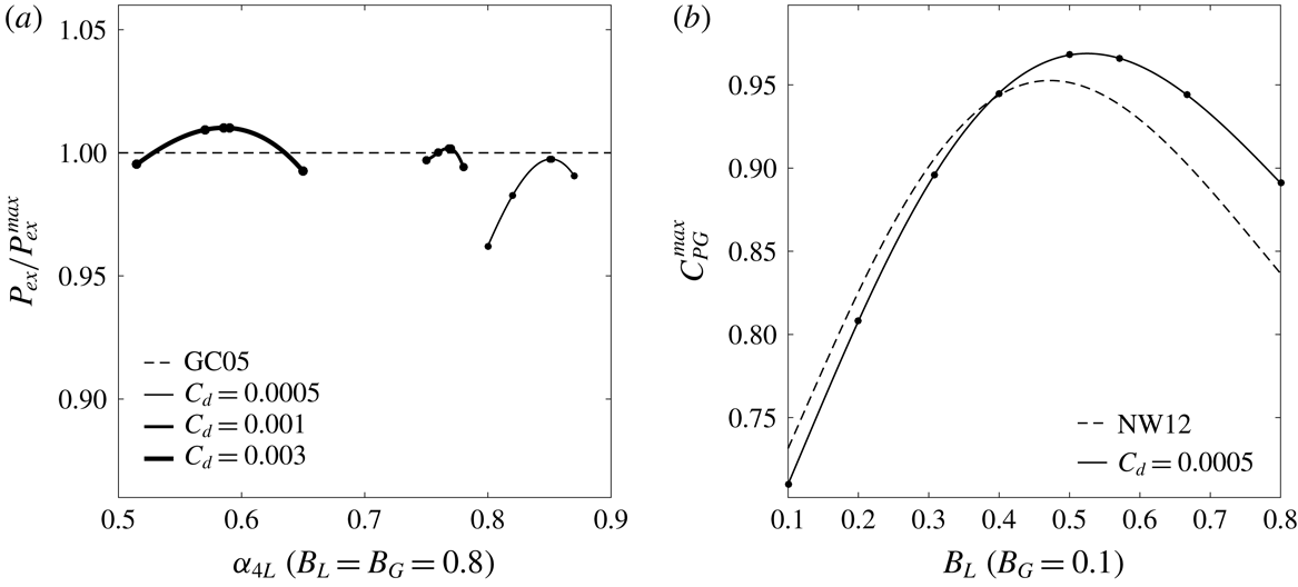
Numerical (solid lines fitted to black markers) and analytical (dashed lines) results for turbines in channels with seabed drag coefficient $C_{d}$ and steady flow driven by constant head difference $\unicode[STIX]{x1D701}=0.0025h_{sC}$ : (a) estimates of maximum extractable power $P_{ex}^{max}$ and (b) variations in maximum global power coefficient $C_{PG}^{max}$ with local blockage $B_{L}$ . Adapted from Bonar et al. (Reference Bonar, Adcock, Venugopal and Borthwick2018).

Convergence of the free surface elevation and depth-averaged velocity results is ensured by comparison with the equivalent results from additional simulations in which the dimensions of the computational grid and model time step are doubled and halved. Results from the numerical channel and array models are then shown to compare favourably, despite their different underlying assumptions, with the respective analytical solutions. Estimates of maximum extractable power (i.e. channel potential), $P_{ex}^{max}$ , calculated using much larger arrays ( $B_{L}=B_{G}=0.8$ ) and for three different values of $C_{d}$ , match very well with predictions from the analytical channel model of Garrett & Cummins (Reference Garrett and Cummins2005, GC05) (figure 3 a), whilst the predicted variation in $C_{PG}^{max}$ with $B_{L}$ , calculated using the chosen array ( $B_{G}=0.1$ ) and a very low roughness flow ( $C_{d}=0.0005$ ), agrees reasonably well with that from the frictionless two-scale actuator disc theory of Nishino & Willden (Reference Nishino and Willden2012b , NW12) (figure 3 b). The larger discrepancies found in the latter case are most likely due to the fact that the analytical model assumes a one-dimensional ‘rigid-lid’ flow which is unaffected by the resistance from turbines, whereas the numerical model describes two-dimensional channel flow with a deformable free surface. The largest deviations from two-scale theory are shown to occur at high $B_{L}$ , which is unsurprising, given that the numerical model is known to overestimate the performance of turbines operating with high thrust in steady, low-roughness flow. Despite these differences, however, the combined array and channel model is shown to reproduce satisfactorily the leading-order physics described by both theoretical models, and is therefore suitable for use in describing the effects of local blockage on the performance of tidal turbines operating in rough and oscillatory channel flow.

Figure 4.

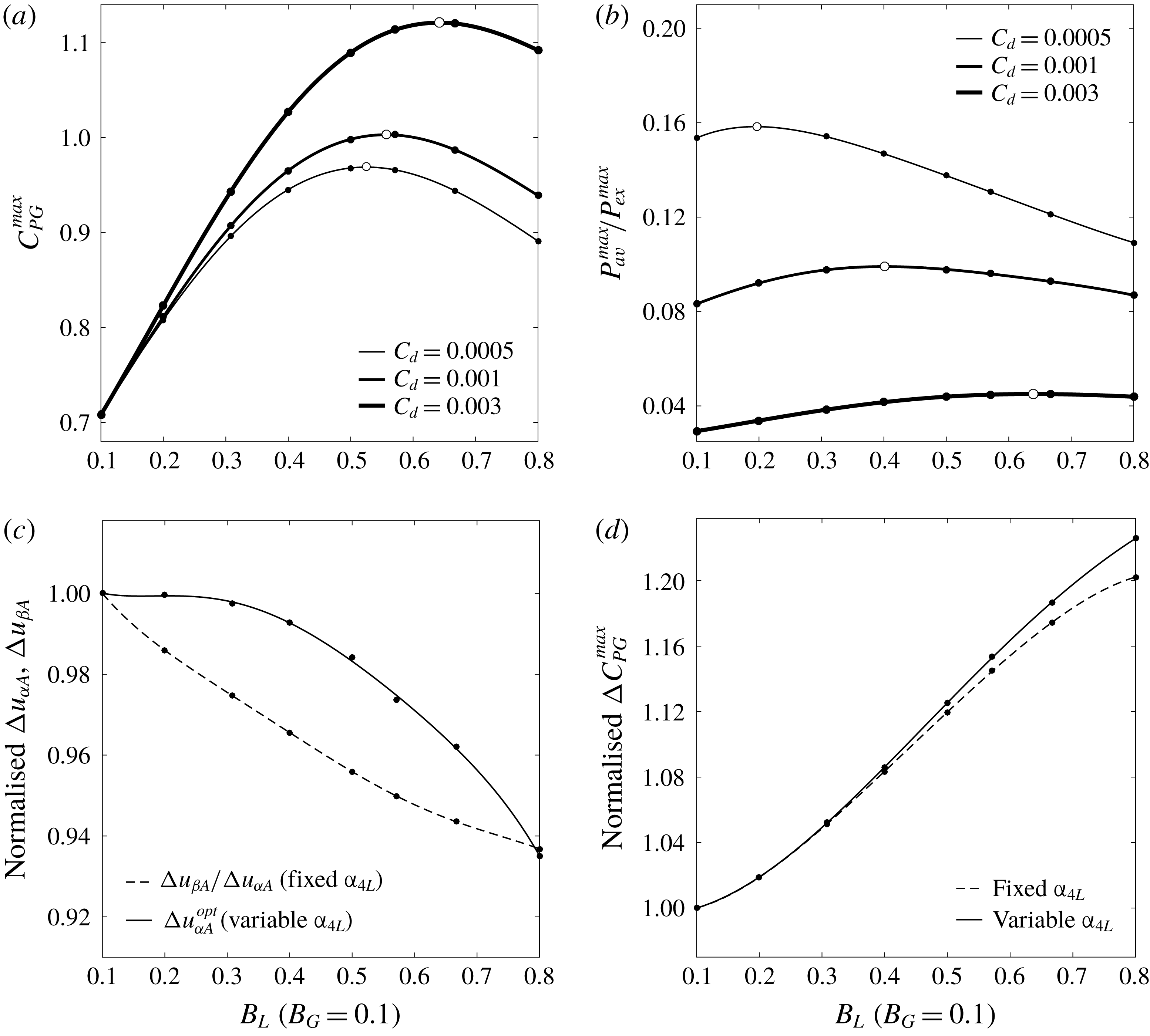
Variations in: (a) maximum global power coefficient $C_{PG}^{max}$ and (b) maximum available power $P_{av}^{max}$ , normalised by maximum extractable power $P_{ex}^{max}$ , with local blockage $B_{L}$ and seabed drag coefficient $C_{d}$ for constant head difference $\unicode[STIX]{x1D701}=0.0025h_{sC}$ . Amounts by which increasing $C_{d}$ from 0.0005 to 0.003 (c) alters the balance between array-scale core and bypass velocities $u_{\unicode[STIX]{x1D6FC}A}$ and $u_{\unicode[STIX]{x1D6FD}A}$ , and thereby $(d)$ enhances $C_{PG}^{max}$ for fixed and variable turbine tunings $\unicode[STIX]{x1D6FC}_{4L}$ .

3 Arrays in steady flow with background roughness

To begin the analysis, the numerical model is used to explore the performance of tidal turbine arrays operating in steady flow with background roughness. A steady channel flow is produced by establishing a constant head difference of $\unicode[STIX]{x1D701}=0.05~\text{m}$ between the two ocean boundaries. The effects of background roughness on the potential for local blockage effects to enhance array performance are then analysed by comparing the optimal arrangements of a given global blockage $(B_{G}=0.1)$ obtained for three different seabed drag coefficients: $C_{d}=0.0005$ , 0.001 and 0.003. (The small value of $\unicode[STIX]{x1D701}$ is chosen to ensure that the model remains stable even for the combination of high turbine thrust and low background roughness; the corresponding values of unexploited streamwise channel velocity and maximum extractable power are $u_{uC}\approx 0.964$ , 0.682 and $0.394~\text{m}~\text{s}^{-1}$ and $P_{ex}^{max}\approx 14.638$ , 10.313 and 5.907 MW.)

Figure 4(a) describes the variations in maximum global power coefficient, $C_{PG}^{max}$ , with local blockage, $B_{L}$ , and seabed drag coefficient, $C_{d}$ , for the chosen $\unicode[STIX]{x1D701}$ and $B_{G}$ . The white markers used to indicate the optimal turbine arrangement for each $C_{d}$ show that the effect of increasing background roughness is to increase both the peak $C_{PG}^{max}$ and the local blockage at which it is achieved: a result which has been previously reported by both Bonar et al. (Reference Bonar, Venugopal, Borthwick and Adcock2016) and Creed et al. (Reference Creed, Draper, Nishino and Borthwick2017).

To understand why this occurs, first consider a single turbine arrangement: $B_{L}=0.5$ , for instance. In flow with very low background roughness ( $C_{d}=0.0005$ ), the maximum $C_{PG}$ of ${\sim}0.9682$ is achieved by tuning the turbines to an $\unicode[STIX]{x1D6FC}_{4L}$ of ${\sim}0.5265$ , whereas in flow with much higher background roughness ( $C_{d}=0.003$ ), the same $\unicode[STIX]{x1D6FC}_{4L}$ produces a $C_{PG}$ of ${\sim}1.0841$ . This performance enhancement is due to the fact that the increase in background roughness affects the array-scale core and bypass flows differently: the natural drag on the flow is proportional to the square of the velocity, and so the same increase in $C_{d}$ slows the faster bypass flow relatively more than it does the slower core flow. Thus, the uniform increase in $C_{d}$ has the effect of increasing the resistance to flow bypassing the array relative to flow through the array, which helps to funnel more flow through the array and thereby enhance its performance. This change in the relative resistance presented to the array-scale core and bypass flows also allows the turbines to be retuned to exert a higher thrust on the incoming flow and thereby further enhance their performance: in the foregoing example, for instance, $C_{PG}$ can be further increased to ${\sim}1.0895$ by retuning the turbines to an $\unicode[STIX]{x1D6FC}_{4L}$ of ${\sim}0.4955$ . For a given turbine arrangement, $B_{L}$ , a uniform increase in background roughness can therefore enhance $C_{PG}$ by means of a ‘resistance boost’, in which the resistance presented to the array-scale bypass flow is increased relative to that presented to the array-scale core flow, and a subsequent ‘retuning boost’, whereby the turbines may then be retuned to present a higher optimal resistance. Although not considered in the present study, it is clear that the same mechanisms could be used to enhance array performance by increasing $C_{d}$ solely in the unexploited part of the channel, so as to increase only the resistance presented to the array-scale bypass flow.

The uniform increase in background roughness is also shown to shift the peak $C_{PG}^{max}$ to a higher local blockage. The reason for this is perhaps best illustrated by figure 4(c,d), which describes the variations with $B_{L}$ in the resistance and retuning boosts which result from increasing $C_{d}$ from 0.0005 to 0.003. For optimally tuned turbines, the difference between the core and bypass velocities increases with $B_{L}$ and so, therefore, do the amounts by which the uniform increase in $C_{d}$ slows the faster bypass flow relatively more than the slower core flow. The dashed line in figure 4(c) represents the ratio of the reductions in the cross-stream-averaged array-scale bypass and core velocities, $u_{\unicode[STIX]{x1D6FD}A}$ and $u_{\unicode[STIX]{x1D6FC}A}$ , which decreases with increasing $B_{L}$ as the relatively faster bypass flow experiences relatively greater slowing. The dashed line in figure 4(d) represents the corresponding resistance boost in $C_{PG}^{max}$ , and demonstrates a resulting increase with $B_{L}$ in the amount by which array performance may thereby be enhanced for a fixed turbine tuning, $\unicode[STIX]{x1D6FC}_{4L}$ . The degree to which the increase in $C_{d}$ slows the array-scale bypass velocity, $u_{\unicode[STIX]{x1D6FD}A}$ , relatively more than the array-scale core velocity, $u_{\unicode[STIX]{x1D6FC}A}$ , increases with $B_{L}$ , which means that the amounts by which the turbines must then be retuned to maximise $C_{PG}$ , and thus $C_{PG}^{max}$ can be enhanced by retuning, must also increase with $B_{L}$ . The solid line in figure 4(c) represents the change in the optimal cross-stream-averaged array-scale core velocity, $u_{\unicode[STIX]{x1D6FC}A}^{opt}$ , which decreases with increasing $B_{L}$ as the optimal turbine resistance increases (in response to the increase in the relative resistance presented to the array-scale bypass flow). The solid line in figure 4(d) represents the sum of the resistance and retuning boosts in $C_{PG}^{max}$ which result from the increase in $C_{d}$ , and comparison with the dashed line in figure 4(d) shows an increase with $B_{L}$ in the potential performance enhancement offered by each mechanism. The amount by which the uniform increase in $C_{d}$ can enhance $C_{PG}^{max}$ thus appears to be an increasing function of $B_{L}$ (figure 4 d), which explains why its addition to the concave function representing the variation in $C_{PG}^{max}$ with $B_{L}$ shifts the peak to a point which is higher in both $C_{PG}^{max}$ and $B_{L}$ (figure 4 a).

Figure 4(b) shows that, for each $C_{d}$ , there is also an optimal turbine arrangement to produce a peak maximum available power, $P_{av}^{max}$ , and that the arrangements which maximise $P_{av}$ and $C_{PG}$ (which is defined as the ratio of $P_{av}$ to channel-scale kinetic energy flux) need not be the same. For $C_{d}=0.0005$ , for instance, $P_{av}^{max}$ begins to reduce with increasing local blockage after its peak at $B_{L}\approx 0.197$ , whereas $C_{PG}^{max}$ continues to increase to a peak at $B_{L}\approx 0.525$ because, as $B_{L}$ increases between these two values (for optimally tuned arrays), the channel-scale kinetic flux decreases faster than $P_{av}$ decreases. The degree to which the arrangements which maximise $P_{av}$ and $C_{PG}$ differ is shown to decrease with increasing $C_{d}$ , however, as the channel-scale kinetic flux is determined less by turbine resistance and increasingly by background roughness.

Trends in $P_{av}$ are found to be similar to those in $C_{PG}$ but with one key difference: whereas $C_{PG}^{max}$ increases with increasing $C_{d}$ , $P_{av}^{max}$ decreases. Figure 4(b) shows that the peak $P_{av}^{max}$ is not only lower in flow with higher background roughness (because with more power dissipated in bed friction, there is less power available to the turbines), but also, as noted by Vennell (Reference Vennell2010), a smaller fraction of the maximum extractable power, $P_{ex}^{max}$ : for $C_{d}=0.003$ , for instance, $P_{av}^{max}$ represents just ${\sim}4.5\,\%$ of $P_{ex}^{max}$ , as compared to ${\sim}15.8\,\%$ of $P_{ex}^{max}$ for $C_{d}=0.0005$ . This is because as $C_{d}$ increases for a given head difference, $P_{ex}^{max}$ decreases as the amount of natural energy dissipation increases, but the natural resistance to flow also increases such that, for a given global blockage with limited capacity to exert thrust on the incoming flow, a smaller fraction of $P_{ex}^{max}$ is available to the turbines. Normalising the variations in $P_{av}^{max}$ with $B_{L}$ by the values obtained for the respective full-width arrays ( $B_{L}=B_{G}=0.1$ ), however, suggests that the available power can be enhanced significantly by exploiting local blockage effects and that, as with the global power coefficient, the potential for performance enhancement increases with increasing natural resistance.

4 Arrays in oscillatory flow with background roughness

The numerical model is now used to explore the performance of tidal turbine arrays operating in oscillatory flow with background roughness: a flow condition which represents a much closer approximation to those in actual tidal channels. The analysis proceeds as before but with simulations now afforded additional relaxation time where necessary, results time-averaged over the last two complete tidal cycles and optimal turbine arrangements sought for different combinations of seabed drag coefficient, $C_{d}$ , and oscillatory tidal forcing, $\unicode[STIX]{x1D709}$ , where $\unicode[STIX]{x1D709}$ represents the amplitude of a single-constituent tide with period $T_{t}=44\,700~\text{s}$ ( ${\sim}12.42$  h). Having previously established the effects of background roughness on the potential for local blockage effects to enhance the maximum available power, $P_{av}^{max}$ (as well as the role of $C_{d}$ in determining both the maximum extractable power, $P_{ex}^{max}$ , and peak $P_{av}^{max}$ ), the effects of fluid inertia are first explored by comparing the variations in $P_{av}^{max}$ with local blockage obtained for a given $C_{d}$ but different values of $\unicode[STIX]{x1D709}$ . The effects of local blockage on array performance are then isolated by normalising the variations in $P_{av}^{max}$ with $B_{L}$ by the values obtained for the respective full-width arrays ( $B_{L}=B_{G}=0.1$ ).

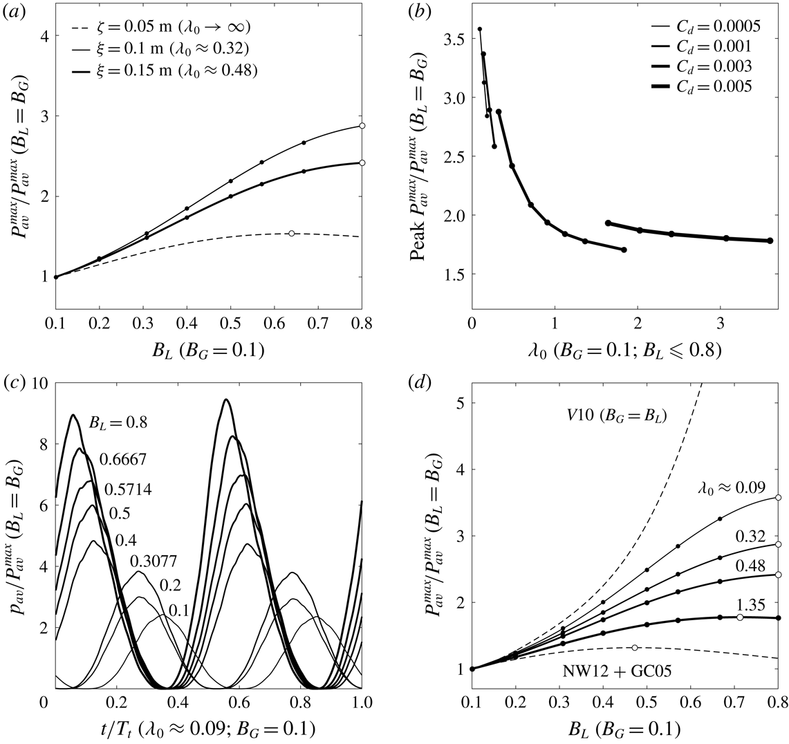
Figure 5(a) describes the variations in normalised maximum available power, $P_{av}^{max}$ , with local blockage, $B_{L}$ , and oscillatory forcing amplitude, $\unicode[STIX]{x1D709}$ , for the chosen global blockage ( $B_{G}=0.1$ ) and a flow with high background roughness ( $C_{d}=0.003$ ). An example variation from the previous steady flow analysis, in which flow is driven by a constant head difference of $\unicode[STIX]{x1D701}=0.05~\text{m}$ , is also included for comparison. The white markers used to indicate the optimal turbine arrangement for each tidal forcing show that, as compared to the power produced by the equivalent full-width arrays, the power available to short, highly blocked arrays increases significantly in oscillatory flow.

Figure 5.

Variations in: (a) maximum available power $P_{av}^{max}$ , normalised by the maximum power available to the equivalent full-width arrays ( $B_{L}=B_{G}$ ), with local blockage $B_{L}$ , constant head difference $\unicode[STIX]{x1D701}$ and oscillatory forcing amplitude $\unicode[STIX]{x1D709}$ for seabed drag coefficient $C_{d}=0.003$ , and (b) normalised peak $P_{av}^{max}$ with natural dynamic balance $\unicode[STIX]{x1D706}_{0}$ (varying $\unicode[STIX]{x1D709}$ for each $C_{d}$ ). Comparisons between: (c) normalised instantaneous power $p_{av}$ (varying in time $t$ over the tidal period $T_{t}$ ) available to eight near-optimally tuned turbine arrangements for $\unicode[STIX]{x1D706}_{0}\approx 0.09$ and $(d)$ numerical (solid lines) and analytical (dashed lines) estimates of the variation in normalised $P_{av}^{max}$ with $B_{L}$ .

To understand why this occurs, first consider how the physics of the problem changes when transitioning from steady to oscillatory flow. In steady flow, the depth and velocity at a given location are constant in time, whereas in oscillatory flow, depth and velocity vary sinusoidally in time with equal but offset phase. Garrett & Cummins (Reference Garrett and Cummins2005) showed that the amount of time by which the peak flow rate lags the peak tidal forcing is determined by the natural dynamic balance, $\unicode[STIX]{x1D706}_{0}$ , which is a dimensionless parameter used to represent, in the absence of turbines, the ratio of drag forces resisting, to inertial forces driving, the channel-scale flow. In the case of quadratic seabed drag, this parameter may be expressed, following Garrett & Cummins (Reference Garrett and Cummins2005), as

(4.1) $$\begin{eqnarray}\unicode[STIX]{x1D706}_{0}=\frac{g\unicode[STIX]{x1D709}\unicode[STIX]{x1D6FC}}{(\unicode[STIX]{x1D714}c)^{2}},\end{eqnarray}$$

with

(4.2a-c ) $$\begin{eqnarray}c=\int _{0}^{l_{C}}\frac{1}{A_{C}}\,\text{d}x,\quad \unicode[STIX]{x1D714}=\frac{2\unicode[STIX]{x03C0}}{T_{t}}\quad \text{and}\quad \unicode[STIX]{x1D6FC}=\int _{0}^{l_{C}}\frac{C_{d}}{hA_{C}^{2}}\,\text{d}x+\frac{1}{2A_{eC}^{2}},\end{eqnarray}$$

in which $c$ is a geometrical factor defined by the length of the channel, $l_{C}$ , and the cross-sectional area of the channel-scale flow, $A_{C}$ ; $\unicode[STIX]{x1D714}$ is the angular frequency of the tide; and $\unicode[STIX]{x1D6FC}$ is an additional parameter used to represent the natural energy losses due to background roughness and the separation of flow at the channel exit, at which point the cross-sectional area is given by $A_{eC}$ . Garrett & Cummins (Reference Garrett and Cummins2005) then showed that the phase lag between peak tidal forcing and peak flow rate decreases with increasing resistance to flow (with increasing $\unicode[STIX]{x1D706}_{0}$ , in the absence of turbines), but did not consider how the dependence of this phase lag on resistance might affect the flow through an array of turbines which spans only part of the channel cross-section. The two-scale actuator disc theory of Nishino & Willden (Reference Nishino and Willden2012b ) later decribed how partial-width turbine arrays separate the channel-scale flow into array-scale core and bypass flows, but did not explain how these array-scale flows interact under oscillatory tidal forcing. In a more recent study, Garrett & Cummins (Reference Garrett and Cummins2013) demonstrated a potential for partial-width arrays to extract more power from oscillatory flow than from steady flow, but did not examine how the interaction of array-scale core and bypass flows might be affected by changes in the channel’s natural dynamic balance. To the authors’ knowledge, the present study is the first to describe the dynamics of oscillatory flow through an array of turbines partially spanning a tidal channel. Results from the numerical model developed herein show that under oscillatory tidal forcing, the array-scale core and bypass flows oscillate side-by-side but with their peak velocities shifted out of phase. It is this phase shift between the array-scale core and bypass velocities that underlies the significant increase in the power available to short, highly blocked arrays in oscillatory flow.

Figure 6.

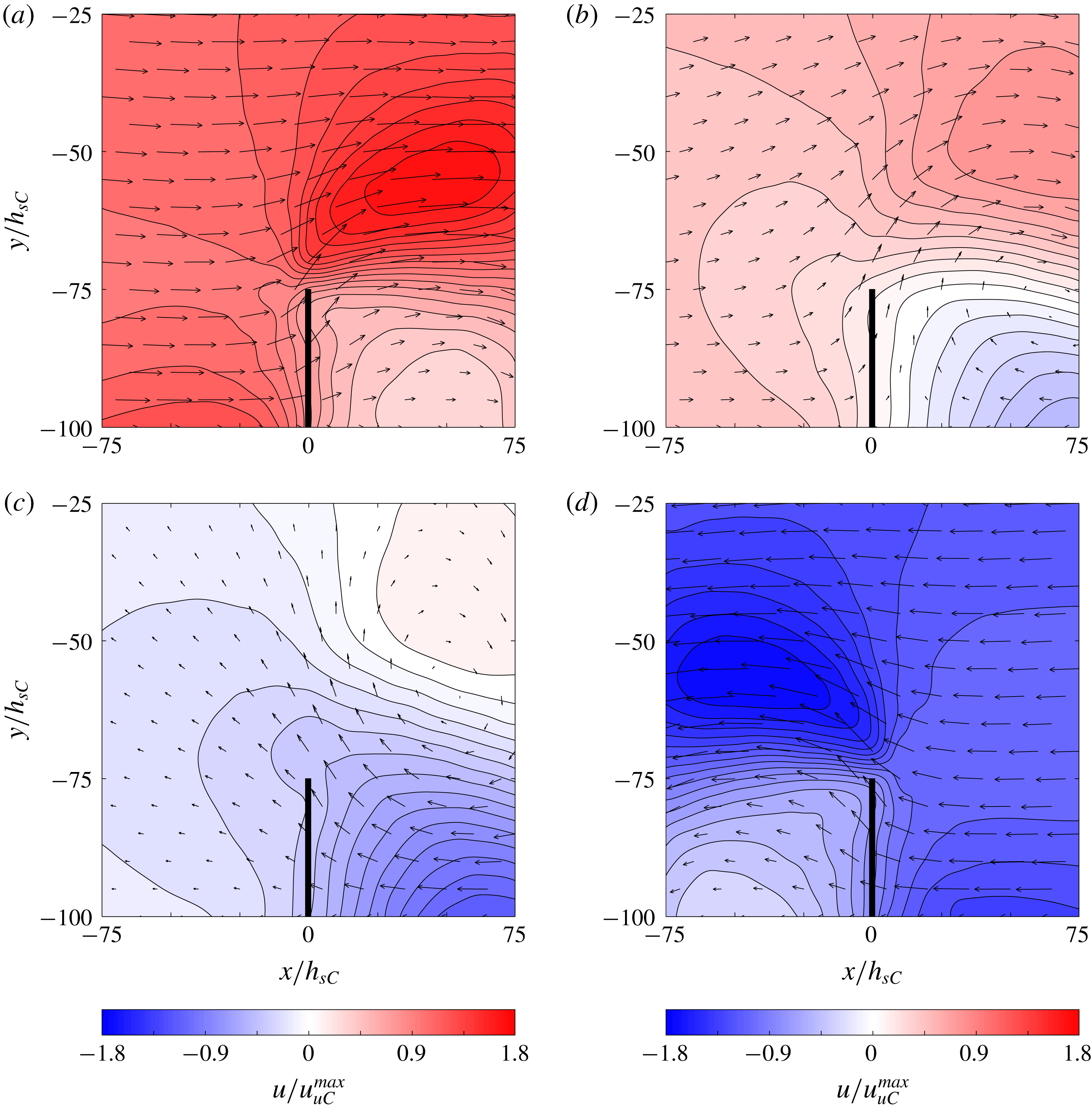
Contours of streamwise depth-averaged velocity $u(x,y)$ , normalised by maximum unexploited streamwise channel velocity $u_{uC}^{max}$ , through and around an array of local blockage $B_{L}=0.8$ within a channel with natural dynamic balance $\unicode[STIX]{x1D706}_{0}\approx 0.09$ at four times during the tidal period $T_{t}$ : (a) $t\approx 0.25T_{t}$ ; (b) $t\approx 0.437T_{t}$ ; (c) $t\approx 0.525T_{t}$ ; $(d)$ $t\approx 0.75T_{t}$ . The position of the turbine array is marked by the thick black vertical line at $x/h_{sC}=0$ , and the thin black arrows illustrate the magnitudes and directions of the corresponding depth-averaged velocity vectors $\boldsymbol{u}(x,y)$ .

The means by which this phase shift enhances array performance is explained as follows. In oscillatory flow, both core and bypass flows experience drag due to background roughness, but the core flow experiences additional drag due to the thrust which is exerted by the turbines. The fact that the resistance to flow is higher in the exploited part of the channel than in the unexploited part of the channel means that the array-scale core flow, which is presented with higher resistance, follows the tidal forcing more closely than does the array-scale bypass flow, which is presented with lower resistance. Now consider, as described in figure 6(a), an instant in the tidal cycle in which the flow is from left to right (in this extreme case, through a near-optimally tuned turbine array with $B_{G}=0.1$ and $B_{L}=0.8$ producing a near-maximum time-averaged available power, $P_{av}^{max}$ , of ${\sim}0.071$  MW in a channel with $C_{d}=0.0005$ ; $\unicode[STIX]{x1D709}=0.1~\text{m}$ ; a maximum unexploited streamwise channel velocity, $u_{uC}^{max}$ , of ${\sim}0.221~\text{m}~\text{s}^{-1}$ ; and $\unicode[STIX]{x1D706}_{0}\approx 0.09$ ). As the tide turns, the array-scale core and bypass flows slow, stop and then begin to flow from right to left. Being phase-shifted ahead, however, the core flow completes this turn before the bypass flow does (figure 6 b), and so when the bypass flow does turn, part of it, rather than attempt to overcome the inertia of the remaining bypass flow and retrace its path directly, diverts into the core region and through the array, thereby enhancing the performance of the turbines (figure 6 c,d). For part of the lagging bypass flow, the region of leading core flow thus temporarily becomes the path of least resistance, which results in a ‘reversal boost’ for the turbines each time the flow changes direction: a ‘kick-start’ at the turn of the tide which produces a stronger array-scale core flow, thereby enabling the turbines to generate more power over the tidal cycle.

In steady flow, array performance is maximised by tuning the turbines to achieve a balance between the local-scale slowing of flow that accompanies energy extraction and the array-scale choking of flow which ultimately limits the amount of power that can be produced. In oscillatory flow, however, it may prove more beneficial, depending on the local blockage ratio and natural flow conditions, to tune the turbines to present a higher resistance to the incoming flow, so as to increase the differences in amplitude and phase between the array-scale core and bypass velocities, and thereby ensure a greater funnelling of array-scale bypass flow through the array when the tide turns. The amount by which the resulting reversal boost can enhance $P_{av}^{max}$ is shown to increase with both increasing $B_{L}$ (figure 5 c), as the potential to exert high thrusts on the incoming flow increases, and decreasing $\unicode[STIX]{x1D706}_{0}$ (which is reduced herein by lowering both $\unicode[STIX]{x1D709}$ and $C_{d}$ ) (figure 5 b), as the array-scale core and bypass velocities are determined less by natural energy losses and increasingly by turbine resistance.

The array-scale dynamics described by the present numerical model is consistent with the theoretical works of Nishino & Willden (Reference Nishino and Willden2012b ) and Garrett & Cummins (Reference Garrett and Cummins2005). Naturally, however, the effects of the cross-stream diversion and resulting reversal boost cannot be predicted using these one-dimensional channel and array theories: even when coupled with the analytical channel model of Garrett & Cummins (Reference Garrett and Cummins2005, GC05), the two-scale theory of Nishino & Willden (Reference Nishino and Willden2012b , NW12) is unable to capture the two-dimensional array-scale dynamics which produces these significant power enhancements (NW12  $+$  GC05) (figure 5 d). By including a comparison with the combined full-width array and channel model of Vennell (Reference Vennell2010, V10), for which $B_{G}$ is not fixed at 0.1 but is instead set equal to $B_{L}$ and thus varies with it, figure 5(d) shows that for sufficiently high $B_{L}$ and sufficiently low $\unicode[STIX]{x1D706}_{0}$ , the amount by which the reversal boost mechanism can enhance the available power is comparable to the amount by which the power could be enhanced by filling the remainder of the cross-section with turbines. Figure 5(d) also suggests that, in the absence of a two-dimensional model such as that developed herein, these two coupled one-dimensional models could be used to provide lower and upper bounds on the maximum power available to partial-width arrays of tidal turbines operating in rough and oscillatory channel flow. The amount by which the available power predictions given by these coupled analytical models differ is shown to increase with $B_{L}$ , but remains small for the lower local blockage ratios likely to be used in practice.

5 Discussion and conclusions

Two-scale actuator disc theory has shown that the performance of a tidal turbine array can be enhanced by varying the lateral spacing between the turbines to exploit local blockage effects. However, the ideal flow assumptions behind two-scale theory, in particular those of frictionless and steady flow, make it difficult to extrapolate from the theory to more realistic channel flow conditions. As a first step towards the development of a more comprehensive theoretical model, the present study uses numerical simulations to explore the potential for local blockage effects to enhance the performance of tidal turbines operating in rough and oscillatory channel flow. To be clear, this study does not seek to provide a formal extension to the two-scale theory, or even a comprehensive set of numerical solutions. Rather, the aim is simply to examine, for a specific set of idealised flow conditions, the interaction between the local- and array-scale dynamics described by the theoretical model of Nishino & Willden (Reference Nishino and Willden2012b ) and the channel-scale dynamics previously described by the theoretical model of Garrett & Cummins (Reference Garrett and Cummins2005).

In revisiting the two-scale theory, it is shown that the optimal local blockage is essentially the arrangement that makes it most difficult for flow to pass around the turbines: more specifically, it is the arrangement for which the local blockage effect enables the production of a peak global power coefficient through the application of a near-peak global thrust coefficient. It seems intuitive, then, that the optimal local blockage must depend on the balance of forces driving and resisting the channel flow, the effects of which are not captured by the two-scale actuator disc model. Results from the combined array and channel model developed herein are then used to relax the ideal flow assumptions of two-scale theory, and describe how optimal turbine arrangements change as the flow transitions from frictionless and steady to rough and oscillatory.

The first set of simulations are used to explore how the optimal turbine arrangement and potential for enhanced power capture are affected by changes in channel background roughness. Numerical results suggest that, as described by Bonar et al. (Reference Bonar, Venugopal, Borthwick and Adcock2016) and Creed et al. (Reference Creed, Draper, Nishino and Borthwick2017), the effect of uniformly increasing the background roughness is to increase the resistance to flow around the array relative to that through the array. This change in the relative resistance presented to the array-scale core and bypass flows allows the turbines to be placed closer together, apply a higher global thrust coefficient and thus produce a higher peak global power coefficient. The results also identify different optimal turbine arrangements to produce a peak maximum available power, and show that although the absolute value of this peak available power decreases with increasing background roughness, the potential for local blockage effects to enhance the maximum available power increases as the natural resistance to flow increases and the additional drag due to turbine thrust becomes less significant.

The second set of simulations are used to obtain optimal arrangements for turbines operating in oscillatory channel flow. Numerical results suggest that the potential for local blockage effects to enhance the maximum available power is much greater in oscillatory flow than in steady flow. Under oscillatory tidal forcing, the additional drag due to turbine thrust is found to induce a phase shift between the array-scale core and bypass velocities, which results in the cross-stream diversion of array-scale bypass flow through the array each time the flow changes direction. This kick-start at the turn of the tide is shown to produce a stronger array-scale core flow, which allows the turbines to generate more power over the tidal cycle. These results suggest that in oscillatory flow, tidal turbines should be arranged in short, highly blocked rows and tuned to exert a high thrust on the incoming flow in order to maximise the effect of this ‘reversal boost’ mechanism, which is found to be more pronounced in channels with low ratios of drag to inertial forces.

Herein, numerical simulations are used to describe, for the first time, the combined effects of oscillatory flow and background roughness on the optimal arrangement of tidal turbines and the potential for enhanced power capture. It is important to recognise, however, that whilst these simulations are designed to expand on existing theoretical works, the present numerical model retains a number of simplifying assumptions. The array-scale dynamics described in this study, for instance, are consistent with these earlier theories, but rely on the assumption that array-scale flow phenomena take place much more slowly and over much greater distances than local-scale flow phenomena: an assumption which may not hold fully in more realistic turbulent flow conditions.

The present model also relies on analytical and idealised numerical models of wake mixing. Moreover, although it is used to describe only array-scale wake mixing processes, and not the local-scale wake mixing processes to which turbine performance is expected to be more sensitive, power results are found to depend on the value of the horizontal eddy viscosity coefficient. The sensitivity of the results is found to be lower in the case of steady flow, where a doubling of the value of the eddy viscosity coefficient is found to increase the time-averaged available power but typically by ${<}1\,\%$ . This finding appears to be consistent with the work of Nishino & Willden (Reference Nishino and Willden2012a ), who showed that an increase in the strength of the turbulent mixing downstream of a tidal turbine results in a slight increase in power production. The sensitivity of the results is found to be greater in the case of oscillatory flow, however, where the effects of increased eddy viscosity are less consistent, and a doubling of the chosen value is found to result in changes in peak instantaneous available power which vary, across the range of flow conditions and turbine arrangements considered, from $+2\,\%$ to $-14\,\%$ . Naturally, the largest changes in peak instantaneous power are found where the differences in the array-scale core and bypass velocities are more pronounced: particularly large changes are found, for instance, where the local blockage of the array is very high and the natural dynamic balance of the channel is very low. However, given that the present study focuses primarily on the time-averaged available power, for which the corresponding changes vary only from $+0.4\,\%$ to $-4\,\%$ , the general trends which are identified should be less sensitive to the value of the horizontal eddy viscosity coefficient than the results from individual simulations.

In calculating the value of the horizontal eddy viscosity coefficient, it is assumed, following Kuipers & Vreugdenhil (Reference Kuipers and Vreugdenhil1973) and Borthwick & Barber (Reference Borthwick and Barber1992), that the value should be proportional to the magnitude of the depth-averaged velocity. It is important to recognise, however, that the temporally constant value adopted herein is likely to be too large to capture accurately the mixing of oscillatory array-scale core and bypass flows during the period near the turn of the tide when the velocities drop to zero. The use of a temporally constant horizontal eddy viscosity coefficient is thus likely to have affected the accuracy of the present numerical results, and is expected to account for part of the large increases in available power which are observed in oscillatory channel flow. In future work, it would prove valuable to revisit this problem using a more detailed, and ideally three-dimensional, numerical model in order to describe more accurately the effects of local- and array-scale wake mixing on the performance of partial-width tidal turbine arrays.

Another important limitation is that the present study does not fully consider the effects of tidal frequency on the performance of the partial-width turbine array. Garrett & Cummins (Reference Garrett and Cummins2013) showed that in oscillatory flow, the maximum extractable power depends on the length scale of the array; the velocity scale of the flow; the amount of natural energy dissipation; and the frequency of flow oscillation. A number of these parameters are considered herein but one key variable which is not examined is the ratio of the time required for the flow to oscillate (that is to say, the period of the driving tide) to the time required for the flow to bypass the array (which might be defined in terms of the width of the array and the velocity of the channel-scale flow). If this ratio is large, then the assumption of quasi-steady flow on which actuator disc theory is based should be approximately valid. If the ratio is small or approaches unity, however, then the effects of flow oscillation and array-scale diversion should become significant. The crucial point is that this time-scale ratio does not depend on the turbine arrangement: that is to say, it exists independently of the blockage ratios. The foregoing oscillatory flow analysis considers only a single tidal period, however, which means that the effects of flow oscillation have not been investigated thoroughly. In future work, numerical simulations should also be performed using a number of different tidal frequencies so as to isolate the effects of this time-scale ratio on the potential for enhanced power capture.

Finally, it must be noted that the present set of simulations are focused on the power performance of a single cross-stream row of idealised turbines operating under a specific set of idealised flow conditions. As such, the foregoing analysis does not account for other important practical considerations, which include the efficiency of the energy extraction, the hydrodynamic loading on the turbines and the resulting changes to the natural flow regime. In addition, the present study assumes that turbine tuning is fixed throughout the tidal cycle and thus does not consider time-variable tuning strategies, which could be used to impose power or thrust limits on turbine performance, or perhaps generate more power over the tidal cycle (e.g. Vennell & Adcock Reference Vennell and Adcock2014; Vennell Reference Vennell2016).

Despite these limitations, however, the present study provides key insights into the effects of channel-scale dynamics on the optimal turbine arrangement and potential for enhanced power capture. Building on the works of Garrett & Cummins (Reference Garrett and Cummins2013), Divett (Reference Divett2014), Creed et al. (Reference Creed, Draper, Nishino and Borthwick2017) and Gupta & Young (Reference Gupta and Young2017), results from the foregoing analysis demonstrate the importance of incorporating not only local blockage effects but also background roughness and, particularly, oscillatory flow in models of tidal turbines. The greatest power enhancements are shown to require local blockage ratios which would be difficult to achieve in practice, but the present results suggest that, for channels with low ratios of drag to inertial forces, significantly more power can be produced by packing turbines into a small part of the cross-section than can be produced by evenly distributing the turbines across the channel width.

Perhaps the most important conclusion from this study is that, by assuming that tidal currents are frictionless and steady, actuator disc models may, under certain conditions, such as when the array is short and very highly blocked, and the ratio of drag to inertial forces in the unexploited channel is very low, neglect leading-order physics and, as a result, produce suboptimal turbine arrangements or inaccurate estimates of the maximum available power. Relaxing these ideal flow assumptions reveals a more complicated problem involving continuous mixing between the core and bypass flows, and demonstrates the need for a new theoretical framework to provide a more accurate description of tidal turbine performance. For the problem of partial-width arrays in channels, it is not immediately clear whether or how the effects of array-scale flow diversion could be incorporated within such a framework. However, it may prove useful to employ an electrical analogy (e.g. Cummins Reference Cummins2013; Draper et al. Reference Draper, Adcock, Borthwick and Houlsby2014) to describe the interaction of array-scale core and bypass flows in channels, and begin by exploring the apparent limits set by coupling the simple channel model of Garrett & Cummins (Reference Garrett and Cummins2005) with the one-dimensional full-width and partial-width array models of Garrett & Cummins (Reference Garrett and Cummins2007) and Nishino & Willden (Reference Nishino and Willden2012b ). Detailed numerical simulations, such as those performed herein, should, of course, also be used to provide further insight. More broadly, the results from this study demonstrate that one should be cautious when applying the findings from steady models to unsteady problems. Tidal currents are complex and dynamic systems, and do not simply comprise instances of steady flow, as is often assumed.