1. Introduction and problem statement

Wetting control, especially the dislodgement of small droplets from solid surfaces (or the prevention thereof), arises in various technologies, from droplet actuation to wiperless windscreens and oil/gas transport (for general reviews of wetting see de Gennes, Brochard-Wyart & Quéré (Reference de Gennes, Brochard-Wyart and Quéré2004), Bonn et al. (Reference Bonn, Eggers, Indekeu, Meunier and Rolley2009) and Snoeijer & Andreotti (Reference Snoeijer and Andreotti2013)). Various approaches have been shown to profoundly affect wetting, such as using surfaces of complex topography, vibrating surfaces and thermal effects. We investigate here droplet spreading/dewetting under non-isothermal conditions, partly with these applications in mind, and partly because assumed isothermal conditions are often not achieved in real systems in the first place.

Non-isothermal spreading/dewetting has been well studied for thin droplets using lubrication theory, following pioneering work by Greenspan (Reference Greenspan1977) on the corresponding isothermal problem. A general evolution equation for the drop height was derived and solved by Ehrhard & Davis (Reference Ehrhard and Davis1991) in the limit of vanishing capillary number, wherein, at any time, the entire drop exhibits a quasi-static shape that is affected by Marangoni stresses. In their study, a relation between an apparent angle and contact-line speed is used that limits the spreading/dewetting. They established that spreading is promoted on a cold surface, and that dewetting is promoted on a hot surface, if the surface tension coefficient decreases when the temperature is increased. Subsequent work has studied notably non-uniformly heated substrates (e.g. Bostwick Reference Bostwick2013).

The first aim here is to study non-isothermal spreading/dewetting with effects of finite capillary number (viscous bending), wherein spreading is limited by the conditions in the immediate vicinity of the contact line. The main difficulty here is that the Navier–Stokes equations for Newtonian fluids, with a no-slip condition, generally lead to a non-integrable singularity in wall shear stress at a moving contact line (Moffatt Reference Moffatt1964; Huh & Scriven Reference Huh and Scriven1971). Various contact-line models have been proposed (e.g. Bonn et al. Reference Bonn, Eggers, Indekeu, Meunier and Rolley2009; Snoeijer & Andreotti Reference Snoeijer and Andreotti2013) that are all challenging to implement in computational models, usually because these introduce a length scale that would have to be very small to represent real systems (Sui, Ding & Spelt Reference Sui, Ding and Spelt2014). Some tests indicate similar wetting behaviour by various models (e.g. Sibley et al. Reference Sibley, Nold, Savva and Kalliadasis2015b ). We adopt a slip model here, as this allows us to compare results with advanced theoretical predictions for isothermal droplet spreading (Hocking & Rivers Reference Hocking and Rivers1982) and prior work on non-isothermal spreading (Ehrhard & Davis Reference Ehrhard and Davis1991). Molecular dynamics simulations do suggest that slip plays a role in contact-line motion (Ren & E Reference Ren and E2007). Various slip models have actually been proposed; we use herein the conventional version wherein the tangential component of velocity at the substrate is proportional to the shear rate, as stated explicitly in § 2.

In § 3 we use lubrication theory to establish the interface shape, including an apparent angle, for a constant actual (not apparent) contact angle. Although such an approach has been pursued previously, this appears to be true only for isothermal systems, the analysis for non-isothermal systems usually being studied with lubrication theory in the limit of vanishing capillary number wherein the contact angle is a prescribed function of contact-line speed (for comparisons between these approaches under isothermal conditions, see Hocking (Reference Hocking1992) and Davis (Reference Davis, Batchelor, Moffatt and Worster2000)). In effect, the analysis in § 3 merges those of Hocking (Reference Hocking1983) and Ehrhard & Davis (Reference Ehrhard and Davis1991). The present approach is expected to be valid at sufficiently small slip length values, and is not valid in the limit of the microscopic contact angle ${\it\theta}_{w}\rightarrow 0$ at a fixed slip length (Hocking Reference Hocking1992). Contrary to prior work, we shall not assume the limit of a small Biot number (defined below). It will be shown in subsequent sections that this allows a comparison with results of direct numerical simulations (DNS).

In subsequent sections we use DNS of the full Navier–Stokes equations to go beyond the lubrication limit for thin droplets. For this purpose we extend our computational method (Sui & Spelt Reference Sui and Spelt2013a ) to non-isothermal spreading/dewetting problems. The main objective there is to establish the role of hot and cold surfaces in promoting or retarding spreading for large contact angles. We also include an investigation of the effect of thermal conduction in the solid substrate.

2. Problem definition

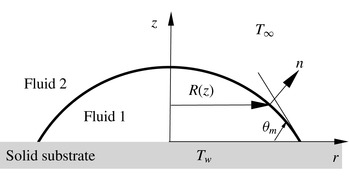
In the DNS we consider axisymmetric spreading and dewetting of a droplet with initial temperature $T_{\infty }$ equal to that of the surrounding fluid on a flat solid surface with homogeneous surface properties and a constant temperature $T_{w}$ (illustrated in figure 1); at the end of this paper, we also consider the effect of heat conduction in a substrate with a finite thickness. Gravity is not considered in the present work, and the fluids are assumed to be Newtonian with constant bulk properties. The initial shape of the drop is chosen to be a spherical cap with a contact-line radius $R$ and a contact angle ${\it\theta}_{ini}$ which equals the microscopic equilibrium contact angle ${\it\theta}_{w}$ . The droplet therefore only spreads/dewets due to the temperature difference between the droplet and the substrate. At late times, the temperature approaches $T_{w}$ throughout, and the droplet will return to its initial shape. We use the DNS here to study wetting/dewetting in this first stage (determining which of these occurs when), which is dominated by thermal effects.

Figure 1.

Problem definition sketch of an axisymmetric droplet on a solid substrate. The contact angle imposed is ${\it\theta}_{w}$ ; the contact angle seen on the macroscale used in this figure is equal to ${\it\theta}_{m}$ , which will differ from ${\it\theta}_{w}$ if interface curvature is large near the contact line. The notation $R(z)$ is introduced for use in § 6.1.

The dependence of the surface tension coefficient on the local temperature is taken to be of the form

(2.1) $$\begin{eqnarray}{\it\sigma}(T)={\it\sigma}_{w}-{\it\gamma}(T-T_{w}),\end{eqnarray}$$

where ${\it\sigma}_{w}$ represents the surface tension coefficient at $T_{w}$ , and ${\it\gamma}$ is a constant that is taken to be positive herein. The surface tension coefficient at $T_{\infty }$ is denoted by ${\it\sigma}_{\infty }$ . The Navier–Stokes equations for incompressible fluids are used, supplemented by an energy equation.

Cylindrical coordinates ( $0\leqslant r\leqslant L_{r},~0\leqslant z\leqslant L_{z}$ ) are employed. At the solid wall ( $z=0$ ) a slip boundary condition, $u_{r}=\hat{{\it\lambda}}\partial u_{r}/\partial z$ , is imposed, with $\hat{{\it\lambda}}$ the slip length and $T=T_{w}$ . Symmetry boundary conditions are imposed at $r=0$ . In the DNS, the flow and temperature are resolved in both fluids, using continuity of velocity, tangential stress and energy flux, and the jump condition for normal stress at the interface. Along the boundaries of the computational domain other than $z=0$ and $r=0$ , zero-normal-gradient boundary conditions are used for velocity and temperature. In the lubrication theory, the flow and temperature in the fluid surrounding the droplet are not resolved, but their effects are modelled by assuming the gas/liquid interface to be shear-free, and through a thermal boundary condition at the interface of the form $-k_{1}\partial T/\partial n=k_{2}(T-T_{\infty })/{\it\delta}$ , with ${\it\delta}$ a length scale representative of the thermal boundary thickness above the drop; the indices 1 and 2 represent liquid and gas properties, respectively.

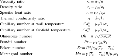
The results are presented in dimensionless form using $R$ as the length scale, ${\it\mu}_{1}R/({\it\sigma}_{w}{\it\theta}_{w}^{3})$ as the time scale, and $T_{w}-T_{\infty }$ as the temperature scale, and the droplet as the reference for fluid properties. This introduces the dimensionless groups listed in table 1.

Table 1.

Definition of dimensionless groups used. The indices 1 and 2 refer to the droplet and exterior fluid, respectively; ${\it\alpha}=k/{\it\rho}c_{p}$ is the thermal diffusivity.

3. Lubrication theory

Lubrication theories have been well developed to model the dynamics of a wide range of thin films (see Craster & Matar Reference Craster and Matar2009 for a review). The pertinent evolution equation for the dimensionless height of a thin droplet reads (Ehrhard & Davis Reference Ehrhard and Davis1991)

(3.1) $$\begin{eqnarray}h_{t}+\frac{1}{r}\left\{\left[\frac{h^{3}}{3}+{\it\beta}h^{2}\right]r\left(h_{rr}+\frac{h_{r}}{r}\right)_{r}+\frac{\widehat{\mathit{Ma}}}{1+Bh^{2}}\left[\frac{h^{2}}{2}+{\it\beta}h\right]rh_{r}\right\}_{r}=0.\end{eqnarray}$$

Here, some rescaling was necessary to facilitate a lubrication approach in this section: the coordinate $r$ is still made dimensionless with $R$ , but for the height $R{\it\theta}_{a}$ is used, time is made dimensionless with ${\it\mu}_{1}R/({\it\sigma}_{w}{\it\theta}_{w}^{3})$ in this section; $B=r_{k}R{\it\theta}_{w}/{\it\delta}$ , $\widehat{\mathit{Ma}}=B{\it\theta}_{w}^{-2}{\it\gamma}(T_{w}-T_{\infty })/{\it\sigma}_{w}=\mathit{Ma}\mathit{Oh}_{w}^{2}B/(\mathit{Pr}{\it\theta}_{w}^{2})$ and ${\it\beta}=\hat{{\it\lambda}}/(R{\it\theta}_{w})$ . The dimensionless variables used here are consistent with those in Hocking (Reference Hocking1983), apart from factors of 3 in the characteristic length and time scales introduced in that prior work having been omitted here. Small differences with the dimensionless evolution equation presented in Ehrhard & Davis (Reference Ehrhard and Davis1991) (their equation (4.8)) are due to different characteristic scales being employed here. The boundary conditions are: at $r=a(t)$ , $h=0$ and $h_{r}=-1$ ; at $r=0$ , $h_{r}=0$ due to symmetry, and we require a constant drop volume $2{\rm\pi}\int _{0}^{a}rh\,\text{d}r={\rm\pi}{\it\chi}/2$ (we keep the parameter ${\it\chi}$ to facilitate comparisons to various prior studies below).

The thermal contribution in (3.1) is entirely due to Marangoni stress. The variation of the surface tension with temperature (2.1) also enters in the normal stress condition, but inspection of the derivation of (3.1) in Ehrhard & Davis (Reference Ehrhard and Davis1991) confirms this to lead to a contribution that is $O({\it\theta}_{w}^{2}\widehat{\mathit{Ma}}/B)$ in (3.1), which is ignored in view of the lubrication approximation made. For internal consistency, the analysis of thermal effects through Marangoni stresses (the thermal term kept in (3.1)) requires $B\gg {\it\theta}^{2}$ .

The isothermal quasi-steady-state drop shape on the scale of the entire drop is readily obtained by ignoring slip, giving the usual result $h_{0}={\it\chi}(a^{2}-r^{2})/a^{4}$ , where $a$ depends on time, the apparent contact angle corresponds to $2{\it\chi}{\it\theta}_{w}/a^{3}$ . We obtain the first correction of $h_{0}$ away from the contact line by substituting $h=h_{0}+h_{1}+\cdots \,$ in (3.1), linearizing in $h_{1}$ , setting $h_{t}={\dot{a}}\partial h_{0}/\partial a$ and imposing the conditions $h_{1}(a)=0$ and $0=\int _{0}^{a}rh_{1}\,\text{d}r=-\!\int _{0}^{a}r^{2}h_{1,r}\,\text{d}r$ . (From (3.1), $h_{1}$ is linear in ${\dot{a}}$ and $\widehat{\mathit{Ma}}$ ; anticipating the result (3.4) of the analysis, this corresponds to an expansion in $1/|\!\ln {\it\beta}|$ and $\widehat{\mathit{Ma}}$ .) This results in

(3.2) $$\begin{eqnarray}\displaystyle rh_{1,r}(r,t) & = & \displaystyle \frac{3}{4}\widehat{\mathit{Ma}}\left((a^{2}-r^{2})\left(\ln \left(\frac{a^{2}-r^{2}}{a^{2}}\right)-\ln \left(\frac{1+\hat{B}(1-r^{2}/a^{2})}{1+\hat{B}}\right)\right)+r^{2}F(\hat{B})\right)\nonumber\\ \displaystyle & & \displaystyle -\,\frac{3}{4}\frac{a^{4}{\dot{a}}}{{\it\chi}^{2}}\left(\ln \left(\frac{a^{2}-r^{2}}{a^{2}}\right)+2\frac{r^{2}}{a^{2}}\right)\end{eqnarray}$$

where $\hat{B}\equiv B{\it\chi}/a^{2}$ and $F(\hat{B})\equiv \hat{B}^{-1}(1-\hat{B}^{-1}\ln (1+\hat{B}))$ , which varies monotonically between $1/2$ ( $\hat{B}\rightarrow 0$ ) and zero ( $\hat{B}\rightarrow \infty$ ). In the isothermal limit, (3.2) agrees exactly with Hocking (Reference Hocking1983). Also, in the limit ${\dot{a}}=0$ , $B\rightarrow 0$ (at small but finite $\widehat{\mathit{Ma}}$ ) it reduces to equation (7.2) in Ehrhard & Davis (Reference Ehrhard and Davis1991). It is seen in (3.2) that thermal effects vanish in the adiabatic limit $B\rightarrow 0$ and in the perfect conduction limit $B\rightarrow \infty$ ; in both these limits the interface temperature $1/(1+Bh)$ becomes a constant (corresponding to the wall and exterior temperature, respectively), resulting in no Marangoni stress. We note though that if $\widehat{\mathit{Ma}}/B$ is kept fixed in the limit $\hat{B}\rightarrow \infty$ , thermal effects remain, with $\hat{B}F(\hat{B})\rightarrow 1$ .

Next, we require the slope as the contact line is approached, which follows as

(3.3) $$\begin{eqnarray}-h_{r}(r\uparrow a)\approx \frac{2{\it\chi}}{a^{3}}+\frac{3}{4}\frac{a^{6}{\dot{a}}}{{\it\chi}^{2}}\left(\ln \left(1-\frac{r}{a}\right)+\ln 2+2\right)-\frac{3}{4}a\widehat{\mathit{Ma}}F(\hat{B}).\end{eqnarray}$$

Evidently, this result for the slope is logarithmically singular as the contact line is approached. This ‘outer region’ result is to be matched to a result for the ‘inner region’, the immediate vicinity of the contact line, wherein this singularity is alleviated by the presence of slip. It should be noted however that the curvature remains singular in this approach, due to isothermal and non-isothermal contributions (the latter are identified in Ehrhard & Davis Reference Ehrhard and Davis1991), as can be inferred from differentiating (3.2). We consider the case wherein ${\dot{a}}\ln {\it\beta}^{-1}$ is not vanishingly small. This usually leads to the requirement of the introduction of a third, ‘intermediate’ region, to match the inner and outer regions (see Cox Reference Cox1986); very recently, such an intermediate region has been demonstrated by Sibley, Nold & Kalliadasis (Reference Sibley, Nold and Kalliadasis2015a ) to be an overlap region of outer and inner regions. For the entire contact-line region it is readily seen from (3.1) that the usual rescaling of the height by the slip length (e.g. Hocking Reference Hocking1983) at this point in the analysis results in the thermal term being preceded by a factor of order ${\it\beta}\widehat{\mathit{Ma}}$ . This is assumed herein to be a very small parameter and is ignored here in the inner region. Therefore, the solution for the inner region is unchanged from that obtained by Hocking (Reference Hocking1983), after changing to the present notation. In the intermediate/overlap region the same argument arises, and thermal contributions are exponentially small, except in a narrow strip at the very outer edge of this region, but this remains small if $\widehat{\mathit{Ma}}$ is small, as assumed here.

To proceed, it is usually noted next that the third power of (3.3) (after linearization in ${\dot{a}}$ and $\widehat{\mathit{Ma}}$ ) yields a term ${\sim}\ln (r-a)$ that matches with a contribution to the result for the intermediate layer obtained by Hocking (Reference Hocking1983). Therefore, the specific function of the interface angle for which the expressions from the outer and intermediate regions are matched is selected by a requirement that the singular terms match exactly. (A similar step occurs in Hocking & Rivers (Reference Hocking and Rivers1982), although there another function of the interface angle is matched because lubrication theory is not used there.) This step has recently been justified by Sibley et al. (Reference Sibley, Nold and Kalliadasis2015a ). Proceeding with matching the third power of the slope at the next order in $r-a$ (which is $O(1)$ ) yields the condition

(3.4) $$\begin{eqnarray}\left(\frac{2{\it\chi}}{a^{3}}\right)^{3}-9a\widehat{\mathit{Ma}}\left(\frac{2{\it\chi}}{a^{3}}\right)^{2}F(\hat{B})=1+9{\dot{a}}\ln \left(\frac{a}{6e{\it\beta}}\right).\end{eqnarray}$$

This agrees with equation (4.1) in Hocking (Reference Hocking1983) if $\widehat{\mathit{Ma}}=0$ (therein ${\it\chi}=4$ , the dimensionless time variable, is three times smaller than ours, so his ${\dot{a}}\equiv \text{d}a/\text{d}t$ corresponds to $3{\dot{a}}$ here; also, his dimensionless slip length corresponds to $3{\it\beta}$ used here). We note that, within the approximations used here, (3.4) can be written in dimensional variables as

(3.5) $$\begin{eqnarray}{\it\theta}_{a}^{3}={\it\theta}_{w}^{3}+9\mathit{Ca}_{cl}\ln \left(\frac{a{\it\theta}_{w}}{6e{\it\lambda}}\right)\end{eqnarray}$$

which agrees exactly with Hocking (Reference Hocking1983), but (3.5) only holds if the apparent angle is defined based on the first two terms on the right-hand side of (3.3). The relation between the angle that the spherical cap makes with the substrate (denoted by ${\it\theta}_{sc}$ ) and this apparent angle is, by comparing (3.5) with (3.4),

(3.6) $$\begin{eqnarray}{\it\theta}_{a}={\it\theta}_{sc}-3{\it\theta}_{w}a\widehat{\mathit{Ma}}F(\hat{B}).\end{eqnarray}$$

If the apparent angle is chosen as the angle obtained by fitting a spherical cap, ${\it\theta}_{a}$ should be eliminated from (3.5) and (3.6). The presence of the dimensionless value of $a$ in these results may seem peculiar, but we recall that this is multiplied by $B$ in the definitions of $\hat{B}$ and $\widehat{\mathit{Ma}}$ , and $B$ is proportional to the length scale $R$ used to make $a$ dimensionless, so $R$ drops out of the product $aB$ and hence out of (3.6).

The matching relations developed above can be cast in the form of the contact-line speed as a power of the difference between apparent and static contact angle assumed by Ehrhard & Davis (Reference Ehrhard and Davis1991) (limit of small capillary and Biot numbers), within the accuracy used, if the power is taken to be $1/3$ ; this has been compared with experiments by Ehrhard (Reference Ehrhard1993), with good results when using an exponent of $1/2.8$ . The use of the present results in the next section – notably (3.5) and (3.6) – is valid for all Biot numbers, and explicit representation of the slip length, under unsteady conditions. We briefly further analyse the present results here, however.

If the initial condition corresponds to the isothermal equilibrium, spreading results on a cold substrate from thermal effects and dewetting on a hot surface (as the first term on both sides in (3.4) then cancel initially), as determined previously by Ehrhard & Davis (Reference Ehrhard and Davis1991). In fact, from (3.4) we conclude that, if the initial condition is such that spreading (dewetting) is expected under isothermal conditions, dewetting may occur if the substrate is cold (hot).

Regarding the rate of spreading/dewetting, after a short-time regime during which the contact-line velocity is constant, $\text{d}a/\text{d}t\sim -\widehat{\mathit{Ma}}$ , (3.4) would not appear to allow for a general power law under non-isothermal conditions. Yet assuming the spherical-cap angle to be very close to the static angle, or both angles to be small, results in $a(t)\sim -\text{sgn}(\widehat{\mathit{Ma}})\,|\widehat{\mathit{Ma}}\,t|^{1/6}$ , where $\widehat{\mathit{Ma}}\,t$ amounts to a rescaling of the time variable such that, in the isothermal viscocapillary time scale ${\sim}{\it\mu}_{1}R/{\it\sigma}_{w}$ , the surface tension ${\it\sigma}_{w}$ is replaced by ${\it\gamma}(T_{w}-T_{\infty })$ . Of course, in the isothermal case, the balance between the first term on the left-hand side with the last term on the right-hand side recovers Tanner’s law for axisymmetric systems ( $a\sim t^{1/10}$ ) (Tanner Reference Tanner1979).

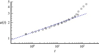
A power law for $a(t)$ has not been predicted previously for non-isothermal systems, to our knowledge (Ehrhard (Reference Ehrhard1993) compared instead with the lubrication theory of Ehrhard & Davis (Reference Ehrhard and Davis1991)). We therefore compare in figure 2(a) the present prediction of $a\sim t^{1/6}$ with the experimental data of Ehrhard (Reference Ehrhard1993) for perfectly wetting silicone oil on a non-isothermal glass surface. We have used here his data for the case with the weakest effects of gravity (data for cases wherein these are stronger differ only marginally). It is seen that a considerable segment of the curve follows a similar power law (as is clear from the corresponding figure in Ehrhard (Reference Ehrhard1993), this power law differs from Tanner’s law). We also note that for a power law of $1/6$ the effect of the initial condition has vanished once the radius is approximately 1.3 its initial value, which corresponds to the start of the experimental data.

Figure 2.

Confirmation of power-law spreading rate as a function of time by comparison with the experiments of Ehrhard (Reference Ehrhard1993) on silicone oil droplets spreading on a cold solid substrate (here $a$ and $t$ are as defined in Ehrhard Reference Ehrhard1993). Symbols are from experiments and the dashed line represents ${\sim}t^{1/6}$ .

When an equilibrium drop shape has almost been reached, such a power law no longer applies. This late-time regime, similar to the exponential late-time regime in isothermal spreading (Hocking Reference Hocking1983), is obtained from linearization (here of (3.4)) in $a(t)-a_{\infty }$ (where $a_{\infty }$ is the equilibrium radius). Allowing for a time-dependent Marangoni number, we obtain

(3.7) $$\begin{eqnarray}a(t)\approx a_{\infty }-G(\infty )+(a_{0}-a_{\infty }+G(\infty ))\text{e}^{-bt}+G(t),\quad G(t)=\int _{0}^{t}c({\it\tau})\text{e}^{-b(t-{\it\tau})}\,\text{d}{\it\tau},\end{eqnarray}$$

where $b=-A_{\infty }^{3}/\!\ln (a_{\infty }/(6e{\it\beta}))$ , $c=(A_{\infty }^{3}-1-9a_{\infty }\widetilde{\mathit{Ma}}A_{\infty }^{2}F)/(9\!\ln (a_{\infty }/(6e{\it\beta})))$ , with $A_{\infty }\equiv 2{\it\chi}/a_{\infty }^{3}={\it\theta}_{ini}/{\it\theta}_{w}$ , where $c$ is allowed to depend on time by a possible time-dependent value of $\widehat{\mathit{Ma}}$ . For constant thermal forcing, this corresponds to an exponential regime with the same exponential $\text{e}^{-bt}$ as in the isothermal limit; thermal effects then only enter in the amplitude. For an exponential thermal forcing $c(t)\sim \text{e}^{-{\it\beta}t}$ , $a(t)$ is a linear combination of $\text{e}^{-bt}$ and $\text{e}^{-{\it\beta}t}$ . There are insufficient experimental data available to validate this late-time regime analysis. Ehrhard (Reference Ehrhard1993) also presented experimental data for paraffin oil with a contact angle of 8° that differ substantially from a power law for perfectly wetting fluids as the equilibrium shape was approached, potentially consistent with the above predictions. But an exponential curve fit has not been pursued here, as several parameters would have to be fitted for a single data set.

The analysis presented here is restricted in many ways – thin drops, a small Marangoni number, the approximate representation of the external temperature field through a prescribed boundary-layer thickness in the interfacial condition for temperature, and the approximate matching procedure adopted. In order to go beyond these restrictions, we turn to full axisymmetric DNS in the subsequent sections, and return to the lubrication theory in the discussion of the DNS results.

4. Computational method for DNS

For DNS beyond the lubrication limit, the finite-volume-based level-set method of Sui & Spelt (Reference Sui and Spelt2013a ) has been extended. The continuous surface tension formulation of the momentum equations is, as under isothermal conditions (e.g. Brackbill, Kothe & Zemach Reference Brackbill, Kothe and Zemach1992), based on a divergence-free velocity field, and is not repeated here. A first difference is the force density term $\boldsymbol{f}(\boldsymbol{x},t)$ in the momentum equation, which represents herein surface tension with Marangoni stresses due to temperature variations (e.g. Herrmann et al. Reference Herrmann, Lopez, Brady and Raessi2008),

(4.1) $$\begin{eqnarray}\boldsymbol{f}(\boldsymbol{x},t)={\it\sigma}(T){\it\kappa}\boldsymbol{{\rm\nabla}}H({\it\phi})+\boldsymbol{{\rm\nabla}}_{s}{\it\sigma}(T)|\boldsymbol{{\rm\nabla}}H({\it\phi})|\end{eqnarray}$$

where ${\it\kappa}$ denotes the interface curvature, ${\it\phi}$ is the level-set function, $H$ is the Heaviside function and $\boldsymbol{{\rm\nabla}}_{s}=(\boldsymbol{I}-\boldsymbol{n}\boldsymbol{n})\boldsymbol{\cdot }\boldsymbol{{\rm\nabla}}$ is the surface gradient operator. The standard approach of Sussman et al. (Reference Sussman, Almgren, Bell, Colella, Howell and Welcome1999) is followed to smoothen the jumps in $H$ over a few grid cells.

A second difference with isothermal approaches is that an energy balance is solved for the temperature field in (4.1). The energy equations for the two fluids involved (along with, in § 7, conduction in the substrate) are combined into a single equation in the same manner as the momentum equation,

(4.2) $$\begin{eqnarray}{\it\rho}c_{p}\left(\frac{\partial T}{\partial t}+\boldsymbol{u}\boldsymbol{\cdot }\boldsymbol{{\rm\nabla}}T\right)=\boldsymbol{{\rm\nabla}}\boldsymbol{\cdot }(k\boldsymbol{{\rm\nabla}}T).\end{eqnarray}$$

In both fluids, the local values of ${\it\rho}c_{p}$ and $k$ are determined as for the density and viscosity in the momentum equation (i.e. using relations of the form $A(\boldsymbol{x},t)=A_{1}+(A_{2}-A_{1})H({\it\phi}(\boldsymbol{x},t))$ ). This formulation is readily derived and shown to account for continuity of temperature and conductive flux at the interface following the arguments as used in the derivation of the continuous surface tension formulation. The solid substrate is represented in § 7 as a third phase with zero velocity and constant physical properties. Viscous heating has been ignored in (4.2) by virtue of the small contact-line speeds considered in the present study; we have conducted tests that include this but found no significant effect on results when $\mathit{Ec}\mathit{Pr}\ll 1$ . We have also assumed the thermal expansion coefficient to be sufficiently small for its effects to be negligible.

A significant difficulty is the large range of length scales involved, which requires excessive resources unless an accurate macroscale model can be formulated (Sui et al. Reference Sui, Ding and Spelt2014), which is not available for non-isothermal systems. In order to simulate flows at more or less realistic values of a dimensionless slip length, $\hat{{\it\lambda}}/R=O(10^{-4})$ , we have incorporated an adaptive mesh refinement tool. Details and extensive validation test results for isothermal conditions can be found in Sui & Spelt (Reference Sui and Spelt2013a ). For non-isothermal conditions we have validated the code by studying thermocapillary migration of a deformable droplet in an infinite quiescent flow with a constant temperature gradient. The terminal migration speed has been obtained analytically by Young, Goldstein & Block (Reference Young, Goldstein and Block1959) for the double limit of small Reynolds and Marangoni numbers. At $\mathit{Re}=0.1$ and $\mathit{Ma}=0.1$ , the difference between the terminal migration speeds from the present numerical simulation and this analytical solution is within 0.09 %. Various comparisons are made between computational results and theoretical analyses throughout this paper. An explicit test from some asymptotic analysis is not available for the problem simulated though, due to differences in boundary conditions used in lubrication theory and the contact-line model in the simulations. A direct validation test for a non-isothermal system with contact lines has been conducted for another system, a cylindrical droplet on a substrate that is kept at a non-uniform temperature, see Sui (Reference Sui2014).

Throughout the following, we have used $r_{d}=r_{v}=r_{c}=0.1$ , $r_{k}=0.01$ and $\mathit{Pr}=1$ in most simulations unless otherwise specified; the values of the remaining dimensionless parameters are stated below, where appropriate. We have verified that the instantaneous values of $\mathit{Re}$ and the Péclet number $\mathit{Pe}=\mathit{Re}\mathit{Pr}$ are small. Typically, the domain size is $L_{r}\times L_{z}=1\times 1$ (for small ${\it\theta}_{w}$ ) or $2\times 2$ (for ${\it\theta}_{w}>{\rm\pi}/3$ ). The mesh resolution in the present study is similar to that used in our previous work (Sui & Spelt Reference Sui and Spelt2013a ), which is sufficient to give mesh-converged results.

5. DNS results for moderate contact angles

In this section and the next, we consider spreading and dewetting of droplets on a substrate that is held at constant uniform temperature (which differs from that of the initial temperature in the two fluids). For sufficiently small contact angle values, the DNS results are consistent with those from the lubrication theory of § 3. For instance, a droplet on a cold surface with ${\it\theta}_{ini}={\it\theta}_{w}={\rm\pi}/3$ for $\mathit{Oh}=0.141$ , $\mathit{Ma}=-2.5$ does spread, as predicted by the lubrication theory. The resulting behaviour exhibits also several similarities with isothermal spreading: the velocity field is similar to ordinary wedge flow, and the velocity along the interface is linear in the distance to the contact line, again similar to ordinary wedge flow driven by a wall subject to a slip boundary condition (not shown).

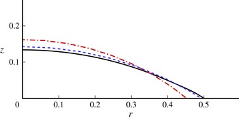
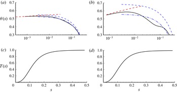
The drop shape is significantly different from that in isothermal spreading, however, as can be seen in figure 3, which is discussed further below. In figure 4 some typical snapshots during spreading on a cold substrate are presented for the angle that the interface makes with the substrate as a function of the distance to the contact line $s$ , for different values of $\mathit{Ma}$ . The corresponding interfacial temperature is also shown. For the largest value of $|\mathit{Ma}|$ , the drop shape is seen to be strongly distorted at $s=O(0.1)$ . The temperature field has only affected part of the droplet at this point, such that the surface tension is not uniform and Marangoni stresses further distort the drop shape; these effects appear to progress in these figures in the form of a wave from the contact line. Qualitatively the same is observed at the lower value of $|\mathit{Ma}|$ (figure 4 a), but of course much weaker there.

Figure 3.

Comparison of the droplet profiles for a cold surface at $\mathit{Oh}=0.141$ , ${\it\theta}_{ini}={\it\theta}_{w}={\rm\pi}/6$ , ${\it\lambda}=0.0004$ , $\mathit{Ca}_{cl}=0.0042$ and $\mathit{Ma}=-25$ . The black solid line represents the DNS result, the red dash-dotted line is obtained from the isothermal theory of Hocking & Rivers (Reference Hocking and Rivers1982) in the outer region, and the blue dashed line is the isothermal theory with apparent contact angle calculated from the present non-isothermal theory.

Figure 4.

Angle that the interface makes with the substrate (a,b) and interfacial temperature (c,d) versus arc length from the contact line during spreading on a cold surface for $\mathit{Oh}=0.141$ , ${\it\theta}_{ini}={\it\theta}_{w}={\rm\pi}/6$ and ${\it\lambda}=0.0004$ : (a,c) $\mathit{Ca}_{cl}=0.0007$ , $\mathit{Ma}=-5$ ; (b,d) $\mathit{Ca}_{cl}=0.0042$ , $\mathit{Ma}=-25$ . Solid lines are from DNS, dashed lines are the intermediate and outer results of Hocking & Rivers (Reference Hocking and Rivers1982), dash-dotted lines are the outer results of Hocking & Rivers (Reference Hocking and Rivers1982) with the apparent angle calculated from (3.5) and (3.6), where $B=0.21$ is inferred from figure 5.

Although close agreement was obtained for isothermal spreading with the theory of Hocking & Rivers (Reference Hocking and Rivers1982) by Sui & Spelt (Reference Sui and Spelt2013a ), we see in figure 4 that this is not so here. The isothermal theory for the outer region is seen to strongly differ from the DNS data, whereas in the intermediate region the DNS data are approached close to the contact line. The comparison in the outer region is reasonable when the apparent angle is calculated from the present non-isothermal theory, as is further confirmed by the comparison of predicted droplet shapes in the outer region shown in figure 3. In the calculation of apparent angle, the value of $B$ is not known a priori; as detailed below, we have inferred and used here $B=0.21$ . We recall also that for isothermal conditions, the corresponding lubrication theory (of Hocking Reference Hocking1983) has been found previously to agree reasonably well with the DNS (Sui & Spelt Reference Sui and Spelt2013a ).

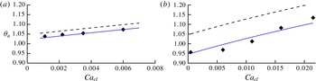
We have measured an apparent angle by fitting a spherical cap through the outer region of the droplet, corresponding to ${\it\theta}_{sc}$ in § 3. The results are shown in figure 5, where also the theoretical prediction by Hocking & Rivers (Reference Hocking and Rivers1982) for the corresponding isothermal system is shown. Under isothermal conditions, this angle may naturally be considered as the apparent angle (e.g. Sui & Spelt Reference Sui and Spelt2013a ), but we now see that with thermocapillarity, ${\it\theta}_{sc}$ attains a considerably lower value than predicted, in line with the snapshots shown in figure 4. Crucially, we find that the non-isothermal lubrication theory, (3.5) and (3.6), gives a reasonable prediction when taking $B=0.21$ (corresponding to ${\it\delta}=O(0.1)$ , which is comparable to the thickness of the droplet). We have also conducted simulations for other parameter values to verify the robustness of this finding, including using $r_{k}=0.1$ instead of 0.01, resulting in similar good agreement in ${\it\theta}_{sc}$ . The thermal boundary layer thickens with $r_{k}$ , so an almost unchanged value for $B$ is not unexpected.

Figure 5.

Apparent angle as a function of the normalized spreading rate. ${\it\lambda}=0.002$ , $\mathit{Oh}=0.141$ , ${\it\theta}_{ini}={\it\theta}_{w}={\rm\pi}/3$ and $\mathit{Ma}=-10$ (a) and $-40$ (b). Symbols are from DNS, the dashed lines are from (3.5) with ${\it\theta}_{a}={\it\theta}_{sc}$ , the solid lines are (3.6), with $B=0.21$ in both cases.

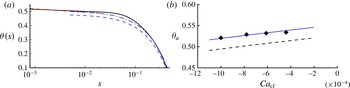
Next, we consider a droplet on a hot surface with ${\it\theta}_{ini}={\it\theta}_{w}$ , which is found here to result in dewetting, consistent with the lubrication theory. Figure 6 shows the interface shape during dewetting and the apparent angle as a function of normalized contact-line speed. We recall here that hitherto no non-isothermal theory is available, except for isothermal spreading, which is seen in this figure not to yield an accurate prediction. Interestingly, the present non-isothermal theory, using the same value for $B$ as in figure 6 (which is for a case of droplet spreading rather than dewetting), leads to a reasonable prediction of the outer shape of the droplet and the apparent angle.

Figure 6.

(a) Angle that the interface makes with the substrate versus arc length from the contact line during dewetting on a hot surface for $\mathit{Oh}=0.141$ , ${\it\theta}_{ini}={\it\theta}_{w}={\rm\pi}/6$ , ${\it\lambda}=0.0004$ , $\mathit{Ca}_{cl}=-0.00087$ and $\mathit{Ma}=5$ . The solid line is from DNS, the dashed lines are the intermediate and outer results of Hocking & Rivers (Reference Hocking and Rivers1982), the dash-dotted line is the outer result of Hocking & Rivers (Reference Hocking and Rivers1982) with the apparent angle calculated from (3.5) and (3.6) with $B=0.21$ . (b) Apparent angle as a function of the normalized contact-line speed, for ${\it\lambda}=0.002$ , $\mathit{Oh}=0.141$ , ${\it\theta}_{ini}={\it\theta}_{w}={\rm\pi}/6$ and $\mathit{Ma}=5$ . Symbols are from DNS, the dashed line is (3.5) with ${\it\theta}_{a}={\it\theta}_{sc}$ , the solid line is from (3.5) and (3.6) with $B=0.21$ .

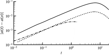
The rate of spreading corresponding to the cases studied in this section is presented in figure 7. The results for spreading and dewetting cases are qualitatively similar. From the lubrication theory in § 3, at short times $\text{d}a/\text{d}t\sim -\widehat{\mathit{Ma}}$ is expected, which is reasonably well approached by the DNS data regarding an initial linear behaviour in time and in $\mathit{Ma}$ (the results for the dewetting case do not fit exactly the results for the wetting case but are for a different static contact angle). At larger times the change in contact-line radius appears to exhibit a power-law dependence in time almost up to the point of maximum displacement, with an exponent close to $5/6$ , especially for the cases of spreading induced by a cold surface.

Figure 7.

Change in contact-line radius versus time for the cases corresponding to the wetting cases of figure 5(a,b) (short dashes and solid line, respectively) and the dewetting case of figure 6(b) (dash-dotted line), all exhibiting a power-law regime.

To conclude, the DNS results indicate that, for modest contact angle values, close to the contact line, the isothermal model remains useful, whereas the outer region is much modified by Marangoni stresses, consistent with non-isothermal lubrication theory, although the predictive capability of the latter for the spreading rate is limited.

6. Large contact angles: spreading∕dewetting reversal

Thus far, the results of lubrication theory and DNS all indicate that, at small contact angles, drops will spread on a surface, or at least, spreading will be promoted, if the substrate is at a temperature lower than the initial temperature of the droplet (referred to herein as a cold wall), and dewet on a hot surface. In our studies we have taken the initial droplet temperature equal to the ambient temperature of the surrounding fluid. We now examine the corresponding behaviour at large contact angles using DNS.

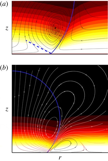
We have found that a hot surface can promote spreading if the contact angle is large: an example is shown in figure 8 for $\mathit{Oh}=0.141$ , ${\it\theta}_{ini}={\it\theta}_{w}=3{\rm\pi}/4$ . The flow pattern for this spreading droplet is seen to involve transport along the interface away from the contact line, which corresponds to the direction of the Marangoni stress. For spreading to occur, an injection-splitting streamline is expected inside the droplet, for the flow along the wall to be directed radially inwards in the frame of reference moving with the contact line.

Figure 8.

Flow field with instantaneous streamlines at $\mathit{Oh}=0.141$ , ${\it\theta}_{ini}={\it\theta}_{w}=3{\rm\pi}/4$ , $\mathit{Ma}=10$ and ${\it\lambda}=0.002$ : (a) near the contact line in a frame of reference moving with the contact line, wherein the blue dashed line identifies the injection-splitting streamline; (b) global flow in a stationary frame.

Figure 9.

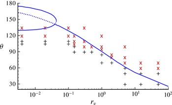
Phase diagram, for $\mathit{Oh}=0.141$ , $\mathit{Ma}=10$ and ${\it\lambda}=0.002$ : ‘ $\times$ ’ represents spreading and ‘ $+$ ’ dewetting. The solid (dashed) lines indicate the prediction presented in § 6.2 based on (6.9) of the critical value of ${\it\theta}={\it\theta}_{w}={\it\theta}_{ini}$ above which spreading (dewetting) on a hot surface is promoted by uniform Marangoni stress alone in a simple wedge model. Note that the role of normal stress is also to promote the spreading on a hot wall, especially at large contact angles, as discussed in § 6.1, and therefore to lower the reversal at large  ${\it\theta}$ .

We have conducted a parametric study to identify the regime boundaries in parameter space, primarily in terms of the viscosity ratio and the contact angle. A phase diagram is shown in figure 9 for a droplet on a hot surface with ${\it\theta}_{ini}={\it\theta}_{w}$ . Spreading is seen to be promoted on a hot surface for large contact angles and a large droplet viscosity (small $r_{v}$ ), and the critical contact angle for spreading/dewetting transition decreases when increasing the external fluid viscosity but is not sensitive to the value of $r_{v}$ for $r_{v}$ less than 0.1 or larger than 10. This means that for realistic liquids droplets will spread on a hot surface when the contact angle is larger than approximately 110°, while a bubble attached to a hot surface will spread when the contact angle defined from the liquid phase is smaller than 120°. At high viscosity ratios, the injection-splitting streamline appears inside the droplet, and the droplet spreads. When the viscosity of the external medium is reduced somewhat, the injection-splitting streamline appears outside the droplet, leading to dewetting. We have confirmed that the phase diagram is robust when $0.5\leqslant \mathit{Ma}\leqslant 40$ , and that the contact line moves in an opposite direction when using a cold instead of a hot wall. This flow diagram is surprisingly similar to that for the direction of thermocapillary translation of an entire droplet on a non-uniformly heated/cooled substrate (Sui Reference Sui2014). In the subsequent subsections we investigate the origin of the spreading/dewetting reversal, not addressed in prior work.

6.1. Role of interfacial normal stress condition: inviscid model

Under isothermal conditions the equilibrium drop shape can be determined by requiring the normal stress jump across the interface to be constant, i.e. the requirement that the surface tension coefficient times the curvature be constant. Under non-isothermal conditions this condition should be modified because the surface tension coefficient depends on the local temperature at the interface, and because Marangoni stresses can drive a (possibly circulating) fluid flow, which in turn can yield a contribution to the normal stress balance. In the lubrication theory presented in § 3, solely the second of these effects is accounted for, the first having dropped out by the lubrication approximation. We have conducted a test case using DNS wherein Marangoni stresses were switched off (by leaving out the last term in (4.1)), and found that a droplet at ${\it\theta}_{ini}={\it\theta}_{w}=120^{\circ }$ still spreads on a hot surface, suggesting that this may be due to the variation in the surface tension coefficient in the normal stress jump.

It is therefore instructive to briefly leave out Marangoni stresses, and investigate instead the direct thermal effect on such an equilibrium drop shape, which is therefore an inviscid analysis. For that purpose, denote the equilibrium interface location by $r=R(z)$ (see figure 1), and assume the surface tension coefficient to be a known function of $z$ only, denoted by ${\it\sigma}(z)$ . The normal stress condition at the interface under equilibrium conditions is then the requirement that ${\it\sigma}(z){\it\kappa}=$ constant ( $\equiv {\it\alpha}$ , say). Here the interface curvature ${\it\kappa}=\boldsymbol{{\rm\nabla}}\boldsymbol{\cdot }\boldsymbol{n}$ , with the normal vector of the interface pointing out of the droplet $\boldsymbol{n}$ having components $n_{r}=1/\sqrt{1+(\text{d}R/\text{d}z)^{2}}$ and $n_{z}=-\text{d}R/\text{d}z/\sqrt{1+(\text{d}R/\text{d}z)^{2}}$ (see figure 1). The above-mentioned stress condition is then obtained as

(6.1) $$\begin{eqnarray}\frac{\text{d}^{2}R}{\text{d}z^{2}}=\frac{1}{R}\left(1+\left(\frac{\text{d}R}{\text{d}z}\right)^{2}\right)-\frac{{\it\alpha}}{{\it\sigma}}\left(1+\left(\frac{\text{d}R}{\text{d}z}\right)^{2}\right)^{3/2}.\end{eqnarray}$$

This equation for $R(z)$ is subject to the boundary condition $\text{d}R/\text{d}z(z=0)=-1/\tan {\it\theta}_{w}$ and the drop volume corresponds to the prescribed volume. This problem is readily solved numerically using the following iterative approach. We start with isothermal cases and place the contact line at $r=1$ , i.e. by setting $R(z=0)=1$ , and then solve the resulting initial-value problem. The value of ${\it\alpha}$ is then obtained by repeatedly solving this ordinary differential equation iteratively until a drop shape is obtained that closes at the top. For non-isothermal cases, the constraint of the contact-line position is replaced by the constraint of the resulting droplet volume being equal to the volume obtained for the isothermal case at the same contact angle. Thus, for non-isothermal cases, we embed the above procedure for isothermal systems in an iterative procedure for the contact-line position subject to the volume constraint. The key result is then the value of $R(z=0)$ : Is this larger or smaller than the isothermal value? We have followed this procedure for the model profile ${\it\sigma}(z)=1\pm 0.5\text{e}^{-10z}$ , wherein the sign corresponds to hot and cold walls (we have also verified that other profiles for ${\it\sigma}(z)$ give similar results – notably a linear dependence on $z$ ).

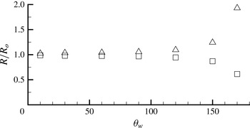
The results are shown in figure 10. At small contact angles, only a comparatively weak effect is observed, consistent with the lubrication theory in § 3, where thermal effects through the normal stress condition were found to be negligible. At large contact angles, a much stronger effect is observed, suggesting that the droplet would spread on a hot wall and dewet on a cold wall. On their own, these thermal effects through the normal stress condition do not cause a spreading/dewetting transition. This is confirmed by the numerical simulation tests wherein we switched off the Marangoni stress: no reversal was observed, but spreading did result in all cases on a hot wall. Therefore, thermal effects through the normal stress jump condition compete with those through Marangoni stress that are predicted by lubrication theory at small contact angles. This is consistent with the results obtained with the DNS shown in figure 9 – a reversal at some critical contact angle.

Figure 10.

Contact-line radius $R$ normalized by its isothermal value at the same drop volume. Result obtained by numerical integrating of (6.1), for ${\it\sigma}(z)=1+0.5\text{e}^{-10z}$ (cold wall, squares) and ${\it\sigma}(z)=1-0.5\text{e}^{-10z}$ (hot wall, triangles).

6.2. Role of Marangoni stress: wedge flow model

In the previous subsection an inviscid mechanism is identified that promotes at large contact angles the reversal of the spreading/dewetting that would otherwise result from Marangoni stress for small contact angles. The mechanism studied there being inviscid, this cannot in itself explain the strong decrease in the critical value of the contact angle at modest to large $r_{v}$ . Instead, the effects of Marangoni stress must be weaker at larger values of $r_{v}$ , or perhaps even reverse themselves upon increasing the contact angle at a fixed value of $r_{v}$ .

In this section, we determine the direction of contact-line motion due to Marangoni stress for Stokes flow in a simplified wedge-shape geometry (e.g. Moffatt Reference Moffatt1964), but for two fluids separated by an interface over which a jump in tangential stress is imposed, as a model of Marangoni stress. Thus we set out to first determine the flow field (resulting from the imposed jump in tangential stress) in a perfect wedge geometry for a stationary substrate, and then use the normal stress condition to determine the first correction in the interface shape caused by the resulting jump in normal stress, and to infer the resulting contact-line motion. The results are then compared with the flow-regime map, figure 9.

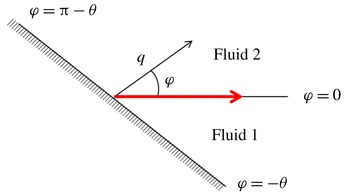
The notation used in this section is defined in figure 11. Polar coordinates ( $q,{\it\varphi}$ ) are used with the origin fixed at the contact line. The interface between the two fluids is at ${\it\varphi}=0$ , with fluid 1 at ${\it\varphi}<0$ and fluid 2 at ${\it\varphi}>0$ . At ${\it\varphi}=0$ , the shear stress ${\it\tau}_{1}$ for the lower fluid differs from ${\it\tau}_{2}$ for fluid 2. The no-slip wall bounding fluid 1 is at ${\it\varphi}=-{\it\theta}$ ; this same wall bounds fluid 2 at ${\it\varphi}={\rm\pi}-{\it\theta}$ . The dependence of the Marangoni stress ${\it\tau}_{1}-{\it\tau}_{2}$ on $q$ resulting from some temperature field can generally be written as a Taylor series, with similar expansions for the stream function. We shall assume that in the far field, on a length scale $\mathscr{L}$ , the Marangoni stress vanishes, and hence the associated velocity and pressure fields. In the following, we shall mainly consider the first term in the series expansion but do indicate how subsequent contributions can be obtained. The interfacial temperature profiles presented in figure 4(c,d) show nonlinear variation with the arc length from the contact line, $s$ , at small and large $s$ , but the main variation may, to a first approximation, be represented by a linear function. We therefore consider mainly the case that ${\it\tau}\equiv {\it\tau}_{1}-{\it\tau}_{2}$ is a constant. The radial coordinate will be taken to have been made dimensionless with $\mathscr{L}$ .

Figure 11.

Problem definition used in § 6.2. Along the interface ${\it\varphi}=0$ a jump in tangential stress is prescribed, represented by the thick (red) arrow.

The general solution for the stream function in fluid 1 can then be obtained from separation of variables,

(6.2) $$\begin{eqnarray}{\it\psi}_{1}(q,{\it\varphi})={\it\mu}_{1}^{-1}{\it\tau}_{1}q^{2}(A_{1}\cos 2{\it\varphi}+B_{1}\sin 2{\it\varphi}+C_{1}{\it\varphi}+D_{1}).\end{eqnarray}$$

The no-slip condition at ${\it\varphi}=-{\it\theta}$ , the no-penetration condition and shear stress condition at ${\it\varphi}=0$ yield

(6.3a−d ) $$\begin{eqnarray}A_{1}=-\frac{1}{4},\quad 4B_{1}=\frac{\cos 2{\it\theta}+2{\it\theta}\sin 2{\it\theta}-1}{2{\it\theta}\cos 2{\it\theta}-\sin 2{\it\theta}},\quad C_{1}=\frac{1}{2}\sin 2{\it\theta}-2B_{1}\cos 2{\it\theta},\quad D_{1}=\frac{1}{4}.\end{eqnarray}$$

The velocity along the interface varies linearly with $q$ ,

(6.4) $$\begin{eqnarray}{\it\mu}_{1}^{-1}{\it\tau}_{1}(2B_{1}+C_{1})q.\end{eqnarray}$$

The flow in fluid 2 is driven by continuity of velocity across the interface. Since this velocity, as we have seen, varies linearly with $q$ , and scales with ${\it\tau}_{1}/{\it\mu}_{1}$ , we find that in fluid 2 the stream function is of the same form as in fluid 1, and shall write this as ${\it\psi}_{2}(q,{\it\varphi})={\it\mu}_{1}^{-1}{\it\tau}_{1}q^{2}(A_{2}\cos 2{\it\varphi}+B_{2}\sin 2{\it\varphi}+C_{2}{\it\varphi}+D_{2})$ . The no-slip condition at ${\it\varphi}={\rm\pi}-{\it\theta}$ , together with the conditions at ${\it\varphi}=0$ corresponding to a no-penetration condition and the radial velocity obtained for fluid 1 above, give for the integration constants in the solution for ${\it\psi}_{2}$ ,

(6.5) $$\begin{eqnarray}\left.\begin{array}{@{}c@{}}\displaystyle A_{2}=\frac{-B_{2}\sin (2{\rm\pi}-2{\it\theta})-2C_{2}({\rm\pi}-{\it\theta})}{\cos (2{\rm\pi}-2{\it\theta})-1},\quad C_{2}=2B_{1}+C_{1}-2B_{2},\quad D_{2}=-A_{2},\\ \displaystyle B_{2}=\frac{(B_{1}+C_{1}/2)(\sin (2{\rm\pi}-2{\it\theta})-2({\rm\pi}-{\it\theta})(\cos (2{\rm\pi}-2{\it\theta})+1))}{2\sin (2{\rm\pi}-2{\it\theta})-2({\rm\pi}-{\it\theta})(\cos (2{\rm\pi}-2{\it\theta})+1)}.\end{array}\right\}\end{eqnarray}$$

The shear stress at ${\it\varphi}=0$ that results from the flow in fluid 2 is $-4A_{2}{\it\mu}_{2}{\it\tau}_{1}/{\it\mu}_{1}$ . Therefore, the jump in the shear stress across the interface is

(6.6) $$\begin{eqnarray}{\it\tau}={\it\tau}_{1}(1+4A_{2}r_{v}).\end{eqnarray}$$

The solution in both fluids is now complete. We note that the stream functions determined here represent a flow that is not directly associated with contact-line motion, but is solely driven by the jump in tangential stress. No contact-line motion occurs in this solution, and the substrate is stationary. The normal stress condition has not been used or needed here: in the assumed limit of large surface tension, interface curvature resulting from a mismatch in normal stress at ${\it\varphi}=0$ would be asymptotically small by assuming surface tension to be asymptotically large. We return to this below, when we relax this limit.

In summary, for a given stress jump ${\it\tau}$ , viscosity ratio and angle ${\it\theta}$ , ${\it\tau}_{1}$ is determined from (6.6) and the coefficients from (6.3a−d ) and (6.5). The above analysis is for an imposed constant Marangoni stress. In the numerical simulations, or in general applications, the Marangoni stress results from the temperature field, and a constant Marangoni stress is only a first approximation. The above analysis can be generalized by considering a Taylor series expansion for the Marangoni stress as a function of $q$ . Each term in such series leads to a problem such as that outlined above: a contribution to the Marangoni stress ${\sim}{\it\mu}_{1}S_{{\it\beta}}q^{{\it\beta}-2}$ leads to a contribution to the stream function $S_{{\it\beta}}q^{{\it\beta}}f_{{\it\beta}}({\it\varphi})$ , where the coefficients in the general solution of $f_{{\it\beta}}({\it\varphi})$ (e.g. Moffatt Reference Moffatt1964) are obtained analogously to the above. Although we proceed with the analysis for constant Marangoni stress below, we do provide at key steps the corresponding general result, to ensure the result is not obscured if the general case is considered.

Spreading might be expected if the velocity at the interface (given by (6.4)) is negative, as this corresponds to the direction for spreading without Marangoni stress (Moffatt Reference Moffatt1964); we generally find this to correspond to ${\it\tau}$ negative (i.e. a cold surface). But this is not conclusive, as no contact-line motion is actually predicted directly by this argument. Rather, as demonstrated below, the normal stress condition for large but finite surface tension yields a first correction of the interface shape by substitution of the flow determined above. In this respect, the present analysis has a parallel in the work of Cox (Reference Cox1986) (around his equation (3.20)), but for a different wedge flow, which is determined in the present problem by Marangoni stress instead of being associated directly (as in Cox Reference Cox1986) with the contact-line motion.

The contribution from the deviatoric stress to the total normal stress ${\it\sigma}_{{\it\varphi}{\it\varphi},i}$ is $({\it\mu}_{i}/{\it\mu}_{1}){\it\tau}_{1}(-4A_{i}\sin 2{\it\varphi}+4B_{i}\cos 2{\it\varphi}+2C_{i})$ ; any further contributions to the Marangoni stress mentioned above ( ${\it\beta}>2$ ) can be determined directly accordingly from the corresponding stream function. The pressure in fluid $i$ is obtained by substituting the stream function in the balance of the radial component of momentum. To confirm that this can be used also when the general expansion of the Marangoni stress in $q$ is accounted for, we first consider the corresponding general result for the pressure,

(6.7) $$\begin{eqnarray}p_{i}=4\frac{{\it\mu}_{i}{\it\tau}_{1}C_{i}}{{\it\mu}_{1}}\ln q+\frac{{\it\mu}_{i}}{{\it\mu}_{1}}\mathop{\sum }_{{\it\beta}=3}^{\infty }\frac{S_{{\it\beta}}q^{{\it\beta}-2}}{{\it\beta}-2}\{{\it\beta}^{2}f_{{\it\beta}}^{\prime }({\it\theta})+f_{{\it\beta}}^{\prime \prime \prime }({\it\theta})\}+{\rm\pi}_{i},\end{eqnarray}$$

where ${\rm\pi}_{i}$ is an integration constant. The length scale $\mathscr{L}$ used in the definition of $q$ has been taken such that at $q\geqslant 1$ Marangoni stresses and the associated pressure disturbance in each fluid vanish. Therefore, ${\rm\pi}_{i}$ must cancel the summation in (6.7), so each term in the summation may give a contribution to ${\rm\pi}_{i}$ . In the following, we concentrate on the leading term on the right-hand side of (6.7), which does not require a contribution to the overall integration constant for it to vanish at $q=1$ .

We obtain for the difference in normal stress across the interface in the positive ${\it\varphi}$ direction, in analogy with equation (3.20) in Cox (Reference Cox1986),

(6.8) $$\begin{eqnarray}\displaystyle & & \displaystyle -4(r_{v}C_{2}-C_{1})\ln q-2C_{1}+2r_{v}C_{2}+4(A_{1}-r_{v}A_{2})\sin 2{\it\theta}-4(B_{1}-r_{v}B_{2})\cos 2{\it\theta}\nonumber\\ \displaystyle & & \displaystyle \quad \qquad \equiv -j({\it\theta},r_{v})\ln q-k({\it\theta},r_{v}),\end{eqnarray}$$

where we have divided by ${\it\tau}_{1}$ . From (6.7) it is seen however that contributions to ${\rm\pi}_{i}$ therein to the pressure from ${\it\beta}>2$ would enter in (6.8) at the same order in $q$ as  $k$ . The present approach is restricted to the leading (logarithmic) term in $q$ , so $k$ is replaced by a general $O(1)$ term henceforth. Equation (6.8) is now equated to the surface tension coefficient times the interfacial curvature, divided by ${\it\tau}_{1}$ , which yields for the angle that the interface makes with the substrate ${\it\theta}(q)$ ,

(6.9) $$\begin{eqnarray}\frac{\partial {\it\theta}}{\partial q}=\widetilde{\mathit{Ma}}\,\left(\frac{{\it\tau}_{1}{\it\sigma}_{w}}{{\it\tau}{\it\sigma}}\right)\{j({\it\theta},r_{v})\ln q+O(1)\}.\end{eqnarray}$$

where $\widetilde{\mathit{Ma}}\equiv {\it\tau}\mathscr{L}/{\it\sigma}_{w}$ , with $\mathscr{L}$ the length scale used to make $q$ dimensionless.

Isothermal droplet spreading is driven by capillarity when the angle between the interface and the wall as the contact line is approached in the outer region exceeds ${\it\theta}_{w}$ . If this apparent angle is lowered by thermal effects, this would reduce the difference with ${\it\theta}_{w}$ that drives spreading, and hence reduce the speed of spreading, just as in the lubrication theory presented in § 3. This could be compensated by thermal effects within the contact-line region, but temperature variation therein would be small due to the smaller size of that region.

The result (6.9) establishes whether the interface is convex or concave as the contact line is approached. It does not establish whether the angle between the interface and the wall is reduced for an arbitrary Marangoni stress distribution along the wedge; that would require extending (6.8)–(6.9) to account for ${\it\beta}>2$ . This is not undertaken here because it would require an estimated temperature distribution along the interface.

Thus it is now conjectured and tested against the numerical simulations, that the sign of the logarithmic term in (6.9), which is dominant at small $q$ , determines whether spreading is promoted. In (6.9), the prefactor ${\it\tau}_{1}/{\it\tau}$ is known from (6.6); the factor ${\it\sigma}/{\it\sigma}_{w}=1+O(\widetilde{\mathit{Ma}})$ should of course be taken consistent with the imposed Marangoni stress, but is reduced to unity in (6.9) at small $|\widetilde{\mathit{Ma}}|$ . Thus, recalling that a positive value of $\widetilde{\mathit{Ma}}$ corresponds to a hot surface, and that the logarithm in (6.9) is negative, a negative value of ${\it\tau}_{1}j/{\it\tau}$ should result in a convex surface of fluid 1 which, according to the hypothesis set out above, would promote spreading on a hot surface.

At small contact angles, the resulting prediction agrees with the lubrication theory. Furthermore, we find that this model predicts a critical contact angle above which the role of Marangoni stress is reversed. We have therefore indicated in figure 9 by solid (dashed) lines ${\it\tau}_{1}j/{\it\tau}=0$ ; above (below) these lines, ${\it\tau}_{1}j/{\it\tau}<0$ , leading to an expectation of spreading being promoted on a hot surface. Good agreement is obtained with the full numerical simulations at intermediate values of $r_{v}$ . We recall here that only a constant Marangoni stress is accounted for in a wedge flow model. Deviations from the prediction such as at small and large $r_{v}$ may be caused by this.

The present model is seen to be of limited use at small values of $r_{v}$ , where it predicts several solution branches. In most cases these are demarcated by singularities at roots of $2{\it\theta}=\tan 2{\it\theta}$ , and in (6.6) (left of and below the first critical line in figure 9, we do obtain ${\it\tau}_{1}j/{\it\tau}>0$ ). These subtleties at low $r_{v}$ , and the overprediction there of the critical contact angle for reversal, are of limited concern, as we recall from § 6.1 that, at such large contact angles, a reversal is also promoted by direct thermal effects through the normal stress condition.

To our knowledge experimental data on (a reversal of) spreading of a drop on a non-isothermal substrate at large contact angles are currently not available, to test the present findings and their applications in, for instance, droplet actuation and microfluidic devices.

7. Effect of conduction inside the substrate

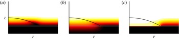
We account herein for the thermal conduction inside the substrate, imposing a constant temperature $T_{w}$ at its lower surface with the droplet on the top surface. A range of values of the solid-to-droplet thermal conductivity ratio $\widehat{r_{k}}=k_{s}/k_{1}$ and thickness of the solid substrate $H$ has been simulated. We take the value of ${\it\rho}c_{p}$ for the solid to be the same as that for the droplet. The typical temperature fields shown in figure 12 show substantial changes in the range of solid conductivity values simulated. We analyse these further below.

Despite the changes in the observed temperature field, tests for droplets with $r_{v}=0.1,1$ and various contact angles have established that heat conduction inside the substrate does not change the phase diagram presented in figure 9 and that for a droplet on a cold surface. The main reason is that, although heat conduction changes the temperature gradient along the interface near the contact line, it does not change its sign. For example, for a droplet on a cold surface, the temperature at the contact line is always lowest compared with the interface temperature close to the contact line, independent of heat conduction inside the substrate. This is different from an evaporating sessile droplet, wherein the interface temperature is determined by both heat conduction and evaporation, and the interface temperature gradient near the contact line can change its sign and therefore cause a reversal of the internal flow circulation, when the ratio of $\widehat{r}_{k}$ is adjusted (Ristenpart et al. Reference Ristenpart, Kim, Domingues, Wan and Stone2007).

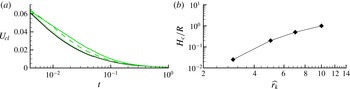
The contact-line dynamics presented in previous sections are approached here at sufficiently large values of the conductivity ratio $\widehat{r}_{k}$ ( $O(100)$ , see figure 12 a). Also, the results are then insensitive to the thickness of the substrate $H$ when this is in the range of $0.1R$ to $2R$ . At lower values of $\widehat{r}_{k}$ , the droplet spreading rate strongly depends on the thickness of the substrate. This is illustrated by figure 13(a), which presents the contact-line speed as a function of time for a droplet on a cold substrate of various thicknesses at $\widehat{r_{k}}=3$ , and compares the results with those for a droplet on a constant-temperature wall. When the deviation in instantaneous spreading speed remains within 2 %, we consider that the substrate is sufficiently thin for the heat conduction to be neglected. The critical thickness $H_{c}$ of the substrate is presented in figure 13(b) versus $\widehat{r_{k}}$ . It is seen that, upon $\widehat{r_{k}}$ decreasing from 10 to 1, $H_{c}$ sharply drops from a length scale similar to the initial droplet radius to a very small value. In the experiments of Ehrhard (Reference Ehrhard1993), a thin glass substrate has been used. There $\widehat{r_{k}}$ was of $O(10)$ , and $H/R$ was less than 0.1; therefore the substrate can be assumed to have had a constant wall temperature. If a substrate is coated with a layer of low thermal conductivity, even when the coating is very thin, the assumption of a constant wall temperature approximation may be invalid.

Figure 12.

Instantaneous temperature profile during droplet spreading on a cold substrate of which the lower surface is kept at constant temperature, with substrate conductivity $\widehat{r_{k}}=100$ (a), 1 (b), 0.01 (c), and substrate thickness $H/R=1/4$ . Other parameters are $r_{k}=0.1$ , $\mathit{Oh}=0.141$ , ${\it\theta}_{ini}={\it\theta}_{w}={\rm\pi}/6$ , ${\it\lambda}=0.0008$ and $\mathit{Ma}=-25$ .

Figure 13.

(a) Time evolution of the contact-line speed. The black solid line is for droplet spreading with $\mathit{Oh}=0.58$ , $\mathit{Ma}=-0.3$ , ${\it\theta}_{ini}={\it\theta}_{w}={\rm\pi}/6$ and ${\it\lambda}=0.02$ . Green lines are results taking into account heat conduction in the substrate with $\widehat{r}_{k}=3$ . The thickness of the substrate is $R/8$ , $R/16$ and $R/40$ for the solid, dashed and dotted line, respectively. (b) Critical thickness of the substrate as a function of ratio of thermal conductivity between the substrate and the droplet. Effect of heat conduction can be neglected below the thickness as explained in the text.

Figure 14.

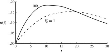
Time evolution of the spreading radius of a droplet on a substrate with a thickness of $R/4$ and thermal conductivities $\hat{r}_{k}=100$ (solid line) and 1 (dashed line). Other parameters are $\mathit{Oh}=0.141$ , $\mathit{Ma}=-40$ , ${\it\theta}_{ini}={\it\theta}_{w}={\rm\pi}/3$ and ${\it\lambda}=0.02$ .

Inspection of the temperature fields in figure 12 confirms the expectation that, when the thermal conductivity of the substrate is comparable to that of the droplet, $|\partial T/\partial r|$ at the contact line can be comparable (or even exceed) $|\partial T/\partial z|$ (this is true even for $\widehat{r_{k}}=10^{-4}$ ). Furthermore, owing to the low wall conductivity, the local wall temperature also changes with time, resulting in a Marangoni number that decreases with time. The juxtaposition of these two effects renders further analysis complex. For the cases considered in the present study, $\partial T/\partial r<0$ , which would promote spreading, however, the decrease in Marangoni number with time weakens spreading. In general, we find that low heat conductivity of the substrate leads to a longer spreading period, because a temperature gradient facilitating spreading can be maintained for longer, but that does not necessarily lead to a larger maximum spreading radius; see figure 14.