2. Derivation procedure of the mILW equation

In this study, we focus on the two-dimensional motion of two layers of incompressible fluids that are stratified according to density in the $z$ direction. The governing equations (Grimshaw, Pelinovsky & Poloukhina Reference Grimshaw, Pelinovsky and Poloukhina2002) in Eulerian coordinates are

(2.1) \begin{equation} \left \{ \begin{aligned} &\frac {\partial u}{\partial x}+\frac {\partial w}{\partial z}=0,\\ &\frac {\partial \rho }{\partial t}+u\frac {\partial \rho }{\partial x}+w\frac {\partial \rho }{\partial z}=0,\\ &\rho \left (\frac {\partial u}{\partial t}+u\frac {\partial u}{\partial x}+w\frac {\partial u}{\partial z}\right )=-\frac {\partial p}{\partial x},\\ &\rho \left (\frac {\partial w}{\partial t}+u\frac {\partial w}{\partial x}+w\frac {\partial w}{\partial z}\right )=-\frac {\partial p}{\partial z}-g\rho . \end{aligned} \right . \end{equation}

Here, the horizontal coordinate axis is at the interface between the two fluid layers, with the vertical axis $z$ being positive in the upward direction. The velocity components in the $x$ and $z$ directions are represented by $u$ and $w$ , respectively; $\rho$ denotes the density, $t$ is the time variable, $p$ represents the fluid pressure, and $g$ is the acceleration due to gravity. Equation (2.1) have a solution corresponding to a motionless ground state, where $u=u_0=0,\ v= v_0=0,\ p=p_0(z),\ \rho =\rho _0(z)$ . The fundamental hydrostatic equilibrium is described by ${{\rm d}p_0}/{{\rm d}z}=-g\rho _0$ . The appropriate boundary conditions associated with $w(z)$ are $w=0$ when $z=h$ and $z=-H$ .

This study investigates the unsteady propagation of nonlinear water waves in a density-stratified fluid system. We adopt a tanh-type continuous density profile (Lamb & Xiao Reference Lamb and Xiao2014) to model the structure characteristic of stratified oceans, where the interface at $z=0$ ensures smooth density continuity:

(2.2) \begin{equation} \rho _0\left (z\right )= \begin{cases} \rho _0 (z ),& h \geqslant {z}\gt {0},\\ \rho _0(0)=\text{constant},& {0}\geqslant z \geqslant {-H}. \end{cases} \end{equation}

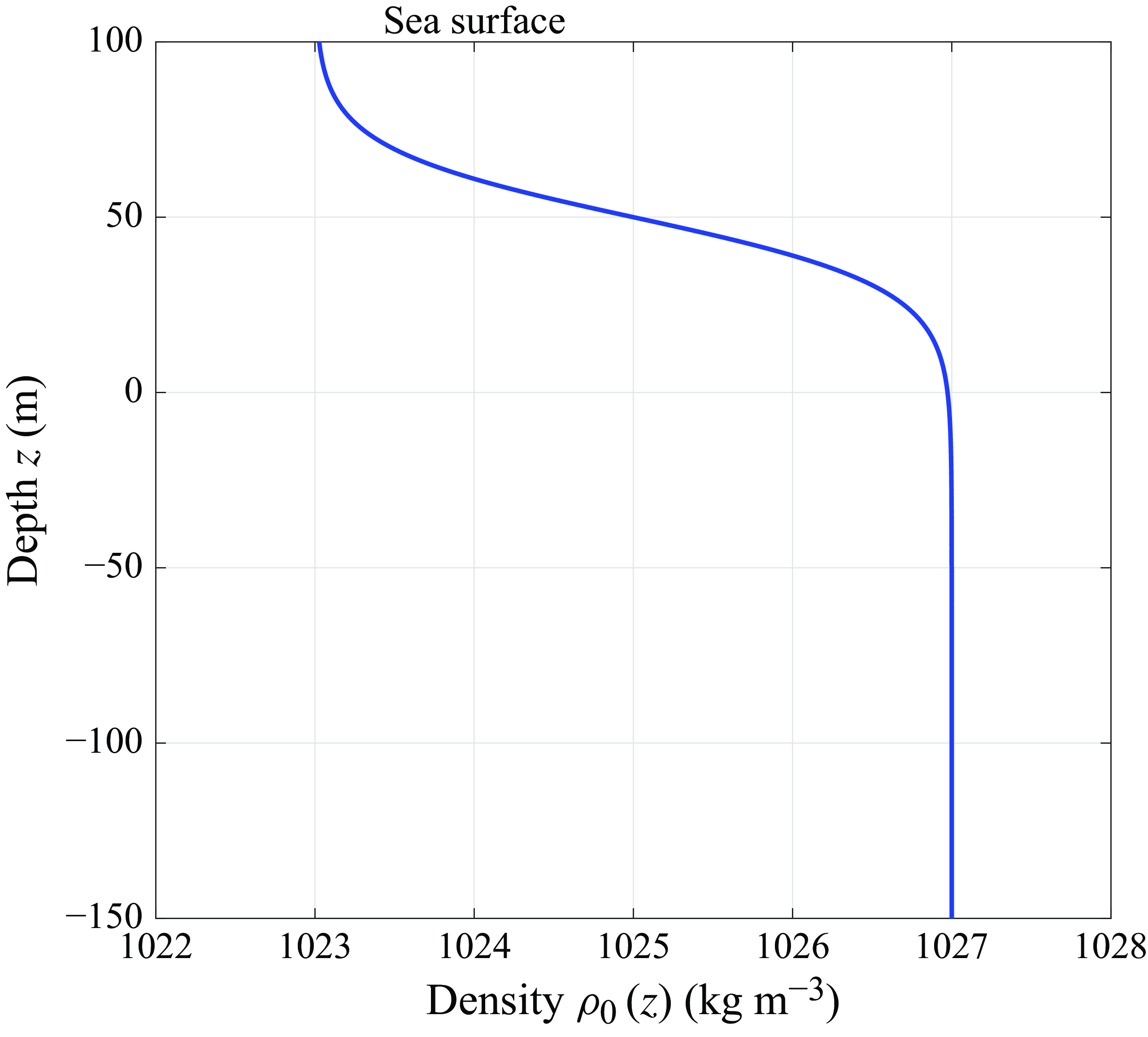
Specifically, the density distribution is defined such that the upper layer ( $h\geqslant {z}\gt {0}$ ) exhibits a vertical variation in density, while the lower layer ( ${0}\geqslant z\geqslant {-H}$ ) remains homogeneous with constant density $\rho _0$ . Figure 1 illustrates the schematic of the density profile model.

Figure 1.

Stratified ocean density profile.

In the derivation of the classical model describing ISWs, Benjamin (Reference Benjamin1967) brought in a small parameter $\epsilon$ . This parameter was used to represent the wave motion at a characteristic spatial scale of the same order as the nonlinearity to balance the effects of nonlinearity and dispersion. However, as the scope of research expanded to include real-world oceanic scenarios with a wider range of wave amplitudes, a significant issue emerged. As the amplitude of the solitary wave increases, the influence of the higher-order nonlinear terms gradually intensifies, resulting in an imbalance between the nonlinear and dispersion effects. When dealing with large-amplitude ISWs, the existing model becomes increasingly inadequate. It fails to accurately capture stronger nonlinear effects or complex soliton dynamics such as modulation instability and high-order soliton interactions. To overcome these limitations and develop a more accurate model that can better account for the behaviour of large-amplitude ISWs, we introduce the following Gardner–Morikawa type transformation in the region $h\geqslant {z}\gt {0}$ (Gardner & Morikawa Reference Gardner and Morikawa1965; Yu, Fu & Yang Reference Yu, Fu and Yang2021):

(2.3) \begin{equation} \begin{aligned} T=\epsilon ^{\tfrac{3}{2}}t,\quad X=\epsilon ^{\tfrac{1}{2}} (x-t). \end{aligned} \end{equation}

Here, both $T$ and $X$ are slow variables, where $T$ denotes the temporal coordinate, and $X$ represents the spatial coordinate. In this way, we obtain the relationship

(2.4) \begin{equation} \begin{aligned} \frac {\partial }{\partial t}=\epsilon ^\frac {3}{2}\frac {\partial }{\partial T}-\epsilon ^\frac {1}{2}\frac {\partial }{\partial X},\quad \frac {\partial }{\partial x}=\epsilon ^\frac {1}{2}\frac {\partial }{\partial X}. \end{aligned} \end{equation}

The perturbation method is a fundamental analytical technique in water wave research (Michele & Renzi Reference Michele and Renzi2020). The essence of the perturbation method is that the complex equations describing a nonlinear wave are reduced to a simple and solvable nonlinear equation by appropriate reductive perturbation expansion. Here, we assume that the velocity components $u,w$ , and pressure $p$ and density $\rho$ , can be asymptotically expanded in terms of a small parameter $\epsilon$ , reflecting their hierarchical contributions across multiple scales. Specifically, these variables are represented as a series of successive approximations:

(2.5) \begin{equation} \left \{ \begin{aligned} &u (X,z,T)=\sum \limits _{i=1}^n\epsilon ^\frac {i}{2}\,u_i (X,z,T),\\ &w (X,z,T)=\sum \limits _{i=1}^n\epsilon ^\frac {i+1}{2}\,w_i (X,z,T),\\ &p (X,z,T)=p_0 (z)+\sum \limits _{i=1}^n\epsilon ^\frac {i}{2}\,p_i (X,z,T),\\ &\rho (X,z,T)=\rho _0(z)+\sum \limits _{i=1}^n\epsilon ^\frac {i}{2}\,\rho _i (X,z,T){,} \end{aligned} \right . \end{equation}

where the subscript indices denote the order of the perturbation terms. This expansion systematically captures the interplay between nonlinear and dispersive effects, ensuring a balanced representation of dominant and higher-order dynamics.

To systematically derive the governing equations, we begin by substituting (2.4) and (2.5) into the fundamental system (2.1). This yields the lowest-order approximate equations for the perturbation parameter $\epsilon$ :

(2.6) \begin{equation} \left \{ \begin{aligned} &\frac {\partial \rho _1}{\partial X}-w_1\frac {\mathrm{d}\rho _0}{\mathrm{d}z}=0,\\ &\frac {\partial u_1}{\partial X}+\frac {\partial w_1}{\partial z}=0,\\ &-\rho _0\frac {\partial u_1}{\partial X}+\frac {\partial p_1}{\partial X}=0,\\ &\frac {\partial p_1}{\partial z}=-g\rho _1. \end{aligned} \right . \end{equation}

Through algebraic elimination of variables $p_1,u_1,\rho_1$ , we isolate the governing equation for $w_1$ :

(2.7) \begin{equation} \begin{aligned} \frac {\partial }{\partial z}\left (\rho _0\frac {\partial w_1}{\partial z}\right )-gw_1\frac {\mathrm{d}\rho _0}{\mathrm{d}z}=0. \end{aligned} \end{equation}

A separation-of-variables approach is then applied to (2.7), assuming solutions of the form

(2.8) \begin{equation} w_1 (X,z,T)=-\phi _1 (z)\,f_X (X,T){,} \end{equation}

where the subscript $X$ denotes a partial derivative with respect to the stretched coordinate $X$ . Substituting (2.8) into (2.6) simplifies the analysis, and it is easy to find that

(2.9) \begin{equation} \begin{aligned} u_1=f\frac {\mathrm{d}\phi _1}{\mathrm{d}z},\quad p_1=\rho _0\frac {\mathrm{d}\phi _1}{\mathrm{d}z}f,\quad \rho _1=-\phi _1\frac {\mathrm{d}\rho _0(z)}{\mathrm{d}z}f. \end{aligned} \end{equation}

Further, the next-order approximate equations for $\epsilon$ can be derived as

(2.10) \begin{equation} \left \{ \begin{aligned} &-\frac {\partial \rho _2}{\partial X}+w_2\frac {\partial \rho _0}{\partial z}=A_1=u_1\frac {\partial \rho _1}{\partial X},\\ &\frac {\partial u_2}{\partial X}+\frac {\partial w_2}{\partial z}=0,\\ &-\rho _0\frac {\partial u_2}{\partial X}+\frac {\partial p_2}{\partial X}=A_2=-\rho _0 u_1\frac {\partial u_1}{\partial X}-\rho _0 w_1\frac {\partial u_1}{\partial z},\\ &\frac {\partial p_2}{\partial z}=-g\rho _2{,} \end{aligned} \right . \end{equation}

leading to the governing equation for $w_2$ :

(2.11) \begin{equation} \begin{aligned} \frac {\partial }{\partial z}\left (\rho _0\frac {\partial w_2}{\partial z}\right )-gw_2\frac {\mathrm{d}\rho _0}{\mathrm{d}z}=-gA_1+\frac {\partial A_2}{\partial z}{.} \end{aligned} \end{equation}

Here,

(2.12) \begin{equation} \begin{aligned} &A_1=u_1\frac {\partial \rho _1}{\partial X}=-\phi _1\frac {\mathrm{d}\phi _1}{\mathrm{d}z}\frac {\mathrm{d}\rho _0}{\mathrm{d}z}ff_X,\\ &A_2=-\rho _0 u_1\frac {\partial u_1}{\partial X}-\rho _0 w_1\frac {\partial u_1}{\partial z}=\left [ -\rho _0^2\left (\frac {\mathrm{d}\phi _1}{\mathrm{d}z} \right )^2 +\rho _0\phi _1\frac {\mathrm{d}^2\phi _1}{\mathrm{d}z^2}\right ]ff_X. \end{aligned} \end{equation}

As a result, we can assume the functional form

(2.13) \begin{equation} w_2=\phi _2 (z)\,f (X,T)\,f_X (X,T), \end{equation}

and $p_2$ , $u_2$ and $\rho _2$ can be solved:

(2.14) \begin{equation} \left \{ \begin{aligned} &u_2=-f^2\frac {\mathrm{d}\phi _2}{\mathrm{d}z},\\ &\rho _2=\frac {\mathrm{d}\rho _0}{\mathrm{d}z}\left (\phi _2+\phi _1\frac {\mathrm{d}\phi _1}{\mathrm{d}z}\right )f^2,\\ &p_2=\left(-g\int \frac {\mathrm{d}\rho _0}{\mathrm{d}z}\left (\phi _2+\phi _1\frac {\mathrm{d}\phi _1}{\mathrm{d}z}\right )\mathrm{d}z\right)\times f^2. \end{aligned} \right . \end{equation}

Finally, we can obtain

(2.15) \begin{equation} \left \{ \begin{aligned} &-\frac {\partial \rho _3}{\partial X}+w_3\frac {\partial \rho _0}{\partial z}=B_1,\\ &\frac {\partial u_3}{\partial X}+\frac {\partial w_3}{\partial z}=0,\\ &-\rho _0\frac {\partial u_3}{\partial X}+\frac {\partial p_3}{\partial X}=B_2,\\ &\frac {\partial p_3}{\partial z}+g\rho _3=B_3, \end{aligned} \right . \end{equation}

where

(2.16) \begin{equation} \left \{ \begin{aligned} &B_1=u_1\frac {\partial \rho _2}{\partial X}+u_2\frac {\partial \rho _1}{\partial X},\\ &B_2=-\rho _0\frac {\partial u_1}{\partial T}-\rho _0 u_1\frac {\partial u_2}{\partial X}-\rho _0 u_2\frac {\partial u_1}{\partial X}-w_1\frac {\partial u_2}{\partial z}-w_2\frac {\partial u_1}{\partial z},\\ &B_3=\rho _0\frac {\partial w_1}{\partial X}. \end{aligned} \right . \end{equation}

Subsequently eliminating $u_3$ , $\rho _3$ and $p_3$ , the governing equation for $w_3$ is

(2.17) \begin{equation} \begin{aligned} \frac {\partial }{\partial z}\left (\rho _0\frac {\partial w_3}{\partial z}\right )-gw_3\frac {\mathrm{d}\rho _0}{\mathrm{d}z}=C, \end{aligned} \end{equation}

where

(2.18) \begin{equation} \begin{aligned} C=-\frac {\partial B_3}{\partial X}-gB_1+\frac {\partial B_2}{\partial z}. \end{aligned} \end{equation}

Substituting (2.16) into (2.18) yields

(2.19) \begin{equation} \begin{aligned} C=C_1f_T+C_2f_{\textit{XXX}}+C_3f^2f_X, \end{aligned} \end{equation}

with

(2.20) \begin{equation} \left \{ \begin{aligned} C_1=&-\frac {\mathrm{d}}{\mathrm{d}z}\left (\rho _0\frac {\mathrm{d}\phi _1}{\mathrm{d}z}\right )\!,\,\,\,\,\,C_2=\rho _0\phi _1,\\ C_3=&-g\frac {\mathrm{d}\rho _0}{\mathrm{d}z} \left [2\frac {\mathrm{d}\phi _1}{\mathrm{d}z}\phi _2+\phi _1\left (\frac {\mathrm{d}\phi _1}{\mathrm{d}z}\right )^2 +\frac {\mathrm{d}\phi _2}{\mathrm{d}z}\phi _1\right ]\\ &-\frac {\mathrm{d}}{\mathrm{d}z} \left (\rho _0\frac {\mathrm{d}\phi _1}{\mathrm{d}z}\frac {\mathrm{d}\phi _2}{\mathrm{d}z}+\phi _1\frac {\mathrm{d}^2\phi _2}{\mathrm{d}z^2}+\phi _2\frac {\mathrm{d}^2\phi _1}{\mathrm{d}z^2}\right ) \!.\\ \end{aligned} \right . \end{equation}

Multiplying both sides of (2.17) by $\phi _1$ , and integrating over $z$ in $[0,h]$ , we can obtain

(2.21) \begin{equation} \begin{aligned} \left .\left [\rho _0\left (\phi _1\frac {\mathrm{d}w_3}{\mathrm{d}z}-\frac {\mathrm{d}\phi _1}{\mathrm{d}z}w_3\right )\right ]\right |_{z=0}^h=\int _{0}^hC\phi _1\,\mathrm{d}z, \end{aligned} \end{equation}

where $\phi _1 (h )=0$ at $z=h$ . Incorporating (2.19) into (2.21) yields a compatibility condition for the perturbation hierarchy:

(2.22) \begin{equation} \begin{aligned} \left .\left [\rho _0\left (\phi _1\frac {\mathrm{d}w_3}{\mathrm{d}z}-\frac {\mathrm{d}\phi _1}{\mathrm{d}z}w_3\right )\right ]\right |_{z=0}^h=a_1f_T+a_2f_{\textit{XXX}}+a_3f^2f_X, \end{aligned} \end{equation}

where

(2.23) \begin{equation} \left \{ \begin{aligned} &a_1=\int _{0}^h{\left [\phi _1\frac {\mathrm{d}}{\mathrm{d}z}\left (\rho _0\frac {\mathrm{d\phi _1}}{\mathrm{d}z}\right )\right ]}\,\mathrm{d}z,\\&a_2=\int _{0}^h{\big (\rho _0\phi _1^2\big )}\,\mathrm{d}z,\\&a_3=\int _{0}^h{-\left \{\phi _1\frac {\mathrm{d}}{\mathrm{d}z} \left (\rho _0\frac {\mathrm{d}\phi _1}{\mathrm{d}z}\frac {\mathrm{d}\phi _2}{\mathrm{d}z}+\phi _1\frac {\mathrm{d}^2\phi _2}{\mathrm{d}z^2}+\phi _2\frac {\mathrm{d}^2\phi _1}{\mathrm{d}z^2}\right )\right \}}\,\mathrm{d}z\\ &\qquad{}-\int _{0}^h{\left \{g\phi _1\frac {\mathrm{d}\rho _0}{\mathrm{d}z} \left [2\frac {\mathrm{d}\phi _1}{\mathrm{d}z}\phi _2+\phi _1\left (\frac {\mathrm{d}\phi _1}{\mathrm{d}z}\right )^2 +\frac {\mathrm{d}\phi _2}{\mathrm{d}z}\phi _1\right ]\right \}}\,\mathrm{d}z.\\ \end{aligned} \right . \end{equation}

In order to capture the multi-scale nature of ISWs in a two-layer ocean, we introduce scaled coordinates that reflect the distinct dynamical behaviours of the upper and lower layers. The upper layer, typically characterised by a thinner depth and smaller density, exhibits faster wave propagation and stronger nonlinear effects, necessitating a finer horizontal scaling. In contrast, the lower layer, with its greater depth and larger density, supports waves with a broader horizontal scale and slower dynamics. To balance the nonlinear and dispersive effects in both layers, we adopt different scaling for the horizontal coordinate in the upper and lower layers, while maintaining a consistent time scaling to ensure the synchronisation of wave evolution across the interface. Specifically, in the lower layer ${0}\geqslant z \geqslant {-H}$ , we adopt the stretching transformations

(2.24) \begin{equation} \begin{aligned} T=\epsilon ^\frac {3}{2}t,\quad X=x-t.\\ \end{aligned} \end{equation}

This is expressible as

(2.25) \begin{equation} \begin{aligned} \frac {\partial }{\partial t}=\epsilon ^\frac {3}{2}\frac {\partial }{\partial T}-\frac {\partial }{\partial X},\quad\frac {\partial }{\partial x}=\frac {\partial }{\partial X}. \end{aligned} \end{equation}

Asymptotic expansions for $u,w,p,\rho$ are then formulated as

(2.26) \begin{equation} \left \{ \begin{aligned} &u(X,z,T)=\sum \limits _{i=1}^n\epsilon ^\frac {i+1}{2}\,U_i(X,z,T),\\ &w(X,z,T)=\sum \limits _{i=1}^n\epsilon ^\frac {i+1}{2}\,W_i(X,z,T),\\ &p (X,z,T)=p_0 (z)+\sum \limits _{i=1}^n\epsilon ^\frac {i+1}{2}\,P_i (X,z,T),\\ &\rho (X,z,T)=\rho _0(z). \end{aligned} \right . \end{equation}

Substituting (2.25) and (2.26) into (2.1), Laplace’s equation for $W_1$ can be expressed as

(2.27) \begin{equation} \begin{aligned} \frac {\partial ^2W_1}{\partial X^2}+\frac {\partial ^2W_1}{\partial z^2}=\textit {O}(\epsilon ), \end{aligned} \end{equation}

with boundary conditions

(2.28) \begin{align} \begin{split} W_1(X,z,T) &= W_0, \quad \quad z =0,\nonumber \\ W_1(X,z,T) & = 0, \quad \qquad z =-H. \end{split} \end{align}

Since (2.27) is Laplace’s equation, by applying the Fourier transform, its inverse transform and the convolution theorem, we are able to obtain the solution of (2.27):

(2.29) \begin{equation} \begin{aligned} W_1 (X,z,T)=\frac {1}{2\pi }\int _{-\infty }^{+\infty }{\mathcal{F}\left ({W_1}|_{z=0}\right )\frac {\textrm{e}^{-kz}-\textrm{e}^{2kH+kz}}{1-\textrm{e}^{2kH}}\,\mathrm{e}^{\mathrm{i}kX}}\,{\rm d}k. \end{aligned} \end{equation}

Here, $\mathcal{F} ({W_1}|_{z=0} )$ represents the Fourier transformation of ${W_1}|_{z=0}$ . Differentiating (2.29) with respect to $z$ gives

(2.30) \begin{equation} \begin{aligned} \frac {\partial W_1 (X,z,T)}{\partial z}=-\frac {1}{2\pi }\int _{-\infty }^{+\infty }k\,{\mathcal{F}\left ({W_1}|_{z=0}\right )\frac {1+\textrm{e}^{2kH+2kz}}{(1-\textrm{e}^{2kH})\,\textrm{e}^{kz}}\,\mathrm{e}^{\mathrm{i}kX}}\,{\rm d}k. \end{aligned} \end{equation}

To establish the continuity condition at the interface $z=0$ , the solutions of the upper and lower layers are matched. Since the lower fluid in our model is specified as a homogeneous medium, pressure continuity automatically holds under this configuration. At the interface $z=0$ , we impose matching conditions based on the continuity of vertical velocity. These arise naturally from the requirement that the fluid motion be dynamically and kinematically compatible across the interface. In particular, since the density is assumed to be continuous at the interface, and the fluids are incompressible, the vertical velocity must also be continuous at $z=0$ . This ensures the smooth transmission of internal wave energy and momentum between the two layers, and is physically justified. By taking the limit as $z$ approaches zero, the following relationships are derived:

(2.31) \begin{align}&\quad \left .\epsilon w_1\right |_{z=0}+\left .\epsilon ^{\frac {3}{2}}w_2\right |_{z=0}+\left .\epsilon ^2w_3\right |_{z=0}=\left .\epsilon W_1\right |_{z=0}, \end{align}

(2.32) \begin{align}& \left .\epsilon\frac {\partial{w_1}}{\partial z}\right |_{z=0}+\left .\epsilon ^{\frac {3}{2}}\frac {\partial w_2}{\partial z}\right |_{z=0}+\left .\epsilon ^2\frac {\partial w_3}{\partial z}\right |_{z=0}=\left .\epsilon \frac {\partial W_1}{\partial z}\right |_{z=0}. \end{align}

From (2.31), we can get

(2.33) \begin{equation} \left .-\phi _1\left (z\right )\,f_X\right |_{z=0}=\left .W_1\right |_{z=0},\quad \left .w_3\right |_{z=0}=0. \end{equation}

According to (2.30) and (2.33), we have

(2.34) \begin{equation} \begin{aligned} \frac {\partial W_1}{\partial z}= \frac {-\epsilon }{4H}\frac {\partial ^2}{\partial X^2}\int _{-\infty }^{+\infty }{ f (X^{\prime },T)\,\phi _1(0) \coth \left [ \frac {\pi }{4H}(X^{\prime }-X)\right ]}\, \mathrm{d}X^{\prime }. \end{aligned} \end{equation}

Considering (2.8), (2.32) and (2.34), it is easy to find that

(2.35) \begin{equation} \begin{aligned} &\phi _1(0)=1,\quad \left .{\frac {\partial \phi _1}{\partial z}}\right |_{z=0}=0,\quad w_3(0)=0,\\ &\left .\frac {\partial w_3}{\partial z}\right |_{z=0}=\frac {-1}{4H}\frac {\partial ^2}{\partial X^2}\int _{-\infty }^{+\infty }{ f (X^{\prime },T)\,\phi _1(0)\coth \left [ \frac {\pi }{4H}(X^{\prime }-X)\right ] }\,\mathrm{d}X^{\prime }. \end{aligned} \end{equation}

Next, substituting (2.35) into (2.22), the new governing equation is obtained:

(2.36) \begin{equation} \begin{aligned} f_T+b_1f^2f_X+b_2f_{\textit{XXX}}+b_3\frac {\partial ^2}{\partial X^2}\,\mathrm{G}(f)=0, \end{aligned} \end{equation}

with $\mathrm{G}(f)= ({-1}/{(4H)})({\partial ^2}/{\partial X^2})\int _{-\infty }^{+\infty }{ f (X^{\prime },T )\,\phi _1(0)\coth [ ({\pi}/{(4H)})(X^{\prime }-X) ]}\, \mathrm{d}X^{\prime }, b_1= ({a_2}/{a_1}),\ b_2= ({a_3}/{a_1}), b_3= ({\rho _{0}(-h)}/{a_1})$ .

Equation (2.36) is a modified model, designated as the mILW equation, which is introduced here to model ISWs in oceanic environments. For brevity, (2.36) is referred to as the mILW model. When the dispersive term $f_{\textit{xxx}}$ vanishes, the mILW equation reduces to the cubic ILW (cILW) equation, as discussed in Naumkin & Sánchez-Suárez (Reference Naumkin and Sánchez-Suárez2018). It reduces to the classical ILW equation when the dispersive term $f_{\textit{XXX}}$ vanishes and the nonlinear term $f^2f_X$ simplifies to $ff_X$ , as documented in Joseph (Reference Joseph1977) and Kubota et al. (Reference Kubota, Ko and Dobbs1978). And when the integral term has $b_3=0$ , it simplifies to the mKdV equation.

The KdV equation is suited for shallow water with weak nonlinearity and long waves. The BO equation assumes an infinitely deep lower layer and is valid for interfacial waves with non-local dispersion, but it lacks applicability in finite-depth ocean environments. The ILW equation bridges the above models by capturing non-local dispersive effects in finite-depth stratified fluids, making it more versatile for oceanographic applications.

Nevertheless, the standard ILW equation includes only quadratic nonlinearity and cannot fully describe the complex structure of stronger nonlinear solitary waves. The mILW equation developed in this work incorporates a third-order nonlinear correction term, enabling the capture of stronger nonlinear behaviours such as amplitude-dependent wave deformation and asymmetrical profiles that are frequently observed in oceanic solitary waves, which are worth further study.

3. Conservation laws

Conservation laws are fundamental to the study of solitary waves, providing critical insights into the underlying dynamics of unsteady wave propagation. These laws, which describe the preservation of quantities such as mass, momentum and energy, are of profound significance in mathematical physics and fluid mechanics, offering a robust framework for analysing wave behaviour and stability (Cebeci & Bradshaw Reference Cebeci and Bradshaw1984; Abreu et al. Reference Abreu, Valencia-Guevara, Huacasi-Machaca and Perez2024).

Building on this foundation, we now turn our attention to identifying conserved quantities for (2.36). By systematically examining the structure of the equation, we aim to derive conservation laws that elucidate the energy and momentum transfer mechanisms inherent in the system.

Assuming that $f(X,T)$ and its derivatives $f_X(X,T)$ , $f_{\textit{XX}}(X,T)$ and $f_{\textit{XXX}}(X,T)$ approach zero as $|X|\rightarrow \infty$ , the conservation of mass is first examined. Equation (2.36) is reformulated as

(3.1) \begin{equation} \begin{aligned} f_T=-b_1f_{\textit{XXX}}-b_2f^2f_X-b_3\frac {\partial ^2}{\partial X^2}\,\mathrm{G}(f), \end{aligned} \end{equation}

and integrating (3.1) with respect to $X$ over the interval $(-\infty ,\infty )$ yields

(3.2) \begin{equation} \begin{aligned} \frac {\mathrm{d}}{\mathrm{d}T}\int _{-\infty }^{+\infty }f\,\mathrm{d}X=0. \end{aligned} \end{equation}

Furthermore, multiplying (3.1) by $f$ and rearranging,

(3.3) \begin{equation} \begin{aligned} ff_T=-b_1ff_{\textit{XXX}}-b_2f^3f_X-b_3f\frac {\partial ^2}{\partial X^2}\,\mathrm{G}(f), \end{aligned} \end{equation}

integrating (3.3) about $X$ from $-\infty$ to $\infty$ , and utilising the following properties of the Hilbert operator,

(3.4) \begin{equation} \begin{aligned} \frac {\partial ^2}{\partial X^2}\mathrm{G}(f)&=\mathrm{G}\left (\frac {\partial ^2f}{\partial X^2}\right)\!,\\ \int _{-\infty }^{+\infty }f\mathrm{G} f\,\mathrm{d}X&=0,\\ \int _{-\infty }^{+\infty }f\mathrm{G} g\,\mathrm{d}X&=-\int _{-\infty }^{+\infty }g\mathrm{G} f\,\mathrm{d}X,\\ \end{aligned} \end{equation}

yields

(3.5) \begin{equation} \begin{aligned} \frac {\mathrm{d}}{\mathrm{d}T}\int _{-\infty }^{+\infty }f^2\,\mathrm{d}X=0{,} \end{aligned} \end{equation}

and the expression for mass $M_1$ ,

(3.6) \begin{equation} \begin{aligned} M_1=\int _{-\infty }^{+\infty }\rho\, \mathrm{d}X, \end{aligned} \end{equation}

where

(3.7) \begin{equation} \begin{aligned} \rho (X,z,T)=\rho _0 (z)+\epsilon ^\frac {1}{2}\,\rho _1 (X,z,T)+\epsilon\, \rho _2 (X,z,T){.}\\ \end{aligned} \end{equation}

It is known above that $\rho _2= ({\mathrm{d}\rho _0}/{\mathrm{d}z}) (\phi _2+\phi _1 ({\mathrm{d}\phi _1}/{\mathrm{d}z}))f^2,\ \rho _1=-\phi _1 ({\mathrm{d}\rho _0(z)}/{\mathrm{d}z})f$ , so the mass conservation can be obtained:

(3.8) \begin{equation} \begin{aligned} \frac {\mathrm{d}M_1}{\mathrm{d}T}=0. \end{aligned} \end{equation}

Similarly, momentum conservation law can be investigated:

(3.9) \begin{equation} \begin{aligned} M_2=\int _{-\infty }^{+\infty }\rho w\,\mathrm{d}X, \end{aligned} \end{equation}

where

(3.10) \begin{equation} \begin{aligned} w (X,z,T)&=\epsilon\, w_1 (X,z,T)+\epsilon ^\frac {3}{2}\,w_2 (X,z,T),\\ w_1 (X,z,T)&=-\phi _1 (z)\,f_X (X,T),\\ w_2 (X,z,T)&=\phi _2 (z)\,f (X,T)\,f_X (X,T), \end{aligned} \end{equation}

so the law of momentum conservation can be derived as

(3.11) \begin{equation} \begin{aligned} \frac {\mathrm{d}M_2}{\mathrm{d}T}=0, \end{aligned} \end{equation}

with

(3.12) \begin{equation} \begin{aligned} M_2&=\int _{-\infty }^{+\infty }\big[\beta _1f_X+\beta _2ff_X+\beta _3f^2f_X+\beta _4f^3f_X \big]\mathrm{d}X,\\ \beta _1&=-\epsilon\, \rho _0(z)\,\phi _1(z),\\ \beta _2&=\epsilon ^{\frac {3}{2}}\,\rho _0(z)\,\phi _2(z)-\epsilon \alpha _1\,\phi _1(z),\\ \beta _3&=-\epsilon ^{\frac {3}{2}}\alpha _1\,\phi _2(z)-\epsilon \alpha _2\,\phi _1(z),\\ \beta _4&=-\epsilon ^{\frac {3}{2}}\alpha _2\,\phi _2(z).\\ \end{aligned} \end{equation}

This analysis provides a comprehensive understanding of the model’s conservation properties. In the context of nonlinear wave models, conservation laws not only validate the mathematical consistency of the governing equations, but also facilitate the derivation of analytical solutions and the interpretation of physical phenomena. These conserved quantities will serve as essential tools for understanding the stability and long-term behaviour of the wave solutions described by the model.

4. Bilinear form and soliton solutions

To gain deeper insights into the propagation dynamics of ISWs, it is essential to solve the nonlinear governing equation (2.36). The study of nonlinear evolution equations has long been a central theme in applied mathematics and theoretical physics, driving the development of numerous analytical and numerical techniques. Hirota’s bilinear method is a powerful tool for constructing multi-soliton solutions for equations of nonlinear evolution. By transforming the nonlinear equation into a bilinear framework through an appropriate variable transformation, Hirota’s bilinear method enables the systematic construction of multi-soliton solutions, making it a cornerstone of soliton theory and nonlinear dynamics. In this section, we employ this method to derive the bilinear form and soliton solutions of (2.36).

The bilinear method has found widespread applications across diverse fields, including mathematical physics, fluid dynamics and optical solitons, due to its ability to handle complex nonlinear interactions with remarkable efficiency. To ensure the physical relevance of the solutions, we impose the condition that the wave profile remains real and finite for all values of the spatial coordinate $X$ and time $T$ . Under this assumption, the solution can be expressed in the form

(4.1) \begin{equation} \begin{aligned} f(X,T)=\mathrm{i}\,\frac {\partial }{\partial X}\ln \frac {g^+(X,T)}{g^-(X,T)}, \end{aligned} \end{equation}

where

(4.2) \begin{equation} \begin{aligned} g^+(X,T)=g(X-2{\rm i}H,T),\quad g^-(X,T)=g(X+2{\rm i}H,T), \end{aligned} \end{equation}

and satisfies $f\rightarrow 0,\ |X|\rightarrow \infty$ , where

(4.3) \begin{equation} \left \{ \begin{aligned} &g\left (X,Y,T\right )=\prod \limits _{n=1}^N\left \{1+\exp\left(\frac {1}{2H}\left [\frac {1}{2H}(\textrm {Im}\,X_n)\left(X-\frac {1}{2H}\right)-X_n^*\right ]\right)\right \}\!,\\ &0\lt \frac {1}{2H}\textrm {Im}\,X_n\lt \pi ,\quad n=1,2,\ldots ,N{.} \end{aligned} \right . \end{equation}

Here, $X_n$ are complex-valued functions dependent on the time variable $T$ , and $X_n^*$ denotes the complex conjugate of $X_n$ .

Using the formula (Yu et al. Reference Yu, Fu and Yang2021)

(4.4) \begin{equation} \begin{aligned} \int _{-\infty }^{+\infty }{\frac {\coth \left [\frac{\pi \lambda }{2}(X^{\prime }-X)\right ]}{\cosh (\lambda \gamma X^{\prime })+\cos (\gamma )}}\,{\rm d}X^{\prime }=-\frac {2\lambda ^{-1}\csc (\gamma )\sinh (\lambda \gamma X)}{\cosh (\lambda \gamma X)+\cos (\gamma )}\quad (0\lt \gamma \lt \pi ), \end{aligned} \end{equation}

$\mathrm{G}(f)$ can be written as

(4.5) \begin{equation} \begin{aligned} \mathrm{G}\left [f\left (X,T\right )\right ]=-\left (\frac {g^+_X}{g^+}+\frac {g^-_X}{g^-}\right )=-\frac {\partial }{\partial X}\mathrm{ln}\left (g^+g^-\right )\!. \end{aligned} \end{equation}

By substituting (4.1) and (4.5) into (2.36), the equation obtained is

(4.6) \begin{equation} \begin{aligned} \mathrm{i}\frac {\partial }{\partial T}\frac {\partial }{\partial X}\mathrm{ln}\frac {g^+}{g^-} +\frac {b_1}{3}\frac {\partial }{\partial X}\left (\!\mathrm{i}\frac {\partial }{\partial X}\mathrm{ln}\frac {g^+}{g^-}\!\right )^3 +b_2\frac {\partial ^3}{\partial X^3}\left (\!\mathrm{i}\frac {\partial }{\partial X}\mathrm{ln}\frac {g^+}{g^-}\!\right )-b_3\frac {\partial ^3}{\partial X^3}\mathrm{ln}\left (g^+g^-\right )=0. \end{aligned} \end{equation}

Integrating this equation with respect to $X$ gives

(4.7) \begin{equation} \begin{aligned} \mathrm{i}\frac {\partial }{\partial T}\mathrm{ln}\frac {g^+}{g^-} +\frac {b_1}{3}\left (\mathrm{i}\frac {\partial }{\partial X}\mathrm{ln}\frac {g^+}{g^-}\right )^3 +b_2\mathrm{i}\frac {\partial ^3}{\partial X^3}\left (\mathrm{ln}\frac {g^+}{g^-}\right )-b_3\frac {\partial ^2}{\partial X^2}\mathrm{ln}\left (g^+g^-\right )=0{,} \end{aligned} \end{equation}

and applying the properties of bilinear operators, we obtain

(4.8) \begin{equation} \begin{aligned} \frac {\partial }{\partial X}\ln \left (\frac {f}{g}\right )&=\frac {D_Xf\boldsymbol{\cdot }g}{fg},\quad\frac {\partial ^2}{\partial X^2}\ln \left (\frac {f}{g}\right )=\frac {D_X^2f\boldsymbol{\cdot }f}{2f^2}-\frac {D_X^2g\boldsymbol{\cdot }g}{2g^2},\\ \frac {\partial ^3}{\partial X^3}\ln \left (\frac {f}{g}\right )&=\frac {D_X^3f\boldsymbol{\cdot }g}{fg}-3\frac {D_X^2f\boldsymbol{\cdot }g}{fg}\frac {D_Xf\boldsymbol{\cdot }g}{fg}+2\left (\frac {D_Xf\boldsymbol{\cdot }g}{fg}\right )^3,\\ \frac {\partial ^2}{\partial X^2}\ln \left (fg\right )&=\frac {D_X^2f\boldsymbol{\cdot }g}{fg}-\left (\frac {D_Xf\boldsymbol{\cdot }g}{fg}\right )^2, \end{aligned} \end{equation}

where

(4.9) \begin{equation} \begin{aligned} D_x^nD_t^m a\boldsymbol{\cdot }b=\left .\left (\frac {\partial }{\partial x}-\frac {\partial }{\partial x_1}\right )^n \left (\frac {\partial }{\partial t}-\frac {\partial }{\partial t_1}\right )^m a(x,t)\boldsymbol{\cdot }b(x_1,t_1)\right |_{x_1=x,\ t_1=t}. \end{aligned} \end{equation}

From (4.1) and (4.5), for clarity and without restricting generality, we adopt $b_1=6b_2$ , which can be achieved by selecting appropriate stratification parameters consistent with observed ocean conditions, as demonstrated in § 5. As a result, the bilinear equation can be derived as

(4.10) \begin{equation} \begin{aligned} \left [\mathrm{i}D_T+\dfrac {1}{6}b_1\mathrm{i}D_X^3-b_3D_X^2\right ]g^+g^-&=0,\\ \left [-\dfrac {1}{2}b_1\mathrm{i}D_X^2+b_3D_X\right ]g^+g^-&=0.\\ \end{aligned} \end{equation}

Assuming that

(4.11) \begin{equation} \begin{aligned} &g^+(X,T)=1+\epsilon g^{(1)+}+\epsilon ^2g^{(2)+}+ {\cdots} +\epsilon ^ng^{(n)+}+ {\cdots} ,\\ &g^-(X,T)=1+\epsilon g^{(1)-}+\epsilon ^2g^{(2)-}+ {\cdots} +\epsilon ^ng^{(n)-}+ {\cdots} , \end{aligned} \end{equation}

for a single soliton solution, substituting (4.11) into the first equation of (4.10), and comparing the coefficients of the first power of $\epsilon$ , we have

(4.12) \begin{equation} \begin{aligned} \epsilon : \mathrm{i}\big(g^{(1)+}-g^{(1)-} \big)_T+\frac {1}{6}b_1\mathrm{i} \big(g^{(1)+}-g^{(1)-} \big)_{\textit{XXX}}-b_3 \big(g^{(1)+}+g^{(1)-} \big)_{\textit{XX}}=0. \end{aligned} \end{equation}

Equation (4.11) can be truncated to $g^{(1)+}(X,T)$ and $g^{(1)-}(X,T)$ , assuming that

(4.13) \begin{equation} \begin{aligned} &g^{(1)-}={\rm e}^{\theta _1+\mathrm{i}\gamma _1}={\rm e}^{\theta _1}(\cos {\gamma _1}+\mathrm{i}\sin {\gamma _1}),\\ &g^{(1)+}={\rm e}^{\theta _1}(\cos {\gamma _1}-\mathrm{i}\sin {\gamma _1}), \end{aligned} \end{equation}

where $\theta _1=k_1X+\omega _1T+\eta _1$ , with $k_1, \omega _1, \eta_1$ as constants. Substituting (4.13) into the bilinear equation (4.12), the dispersion relation is obtained:

(4.14) \begin{equation} \begin{aligned} \omega _1=b_3k_1^2\cot {\gamma _1}-\frac{1}{6}b_1k_1^3. \end{aligned} \end{equation}

By substituting (4.13) into (4.1), the one-soliton solution of (2.36) is derived:

(4.15) \begin{equation} \begin{aligned} f=\frac {2k_1\,{\rm e}^{\theta _1}\sin \gamma _1}{1+{\rm e}^{2 \theta _1}+2 {\rm e}^{\theta _1}\cos {\gamma _1}}. \end{aligned} \end{equation}

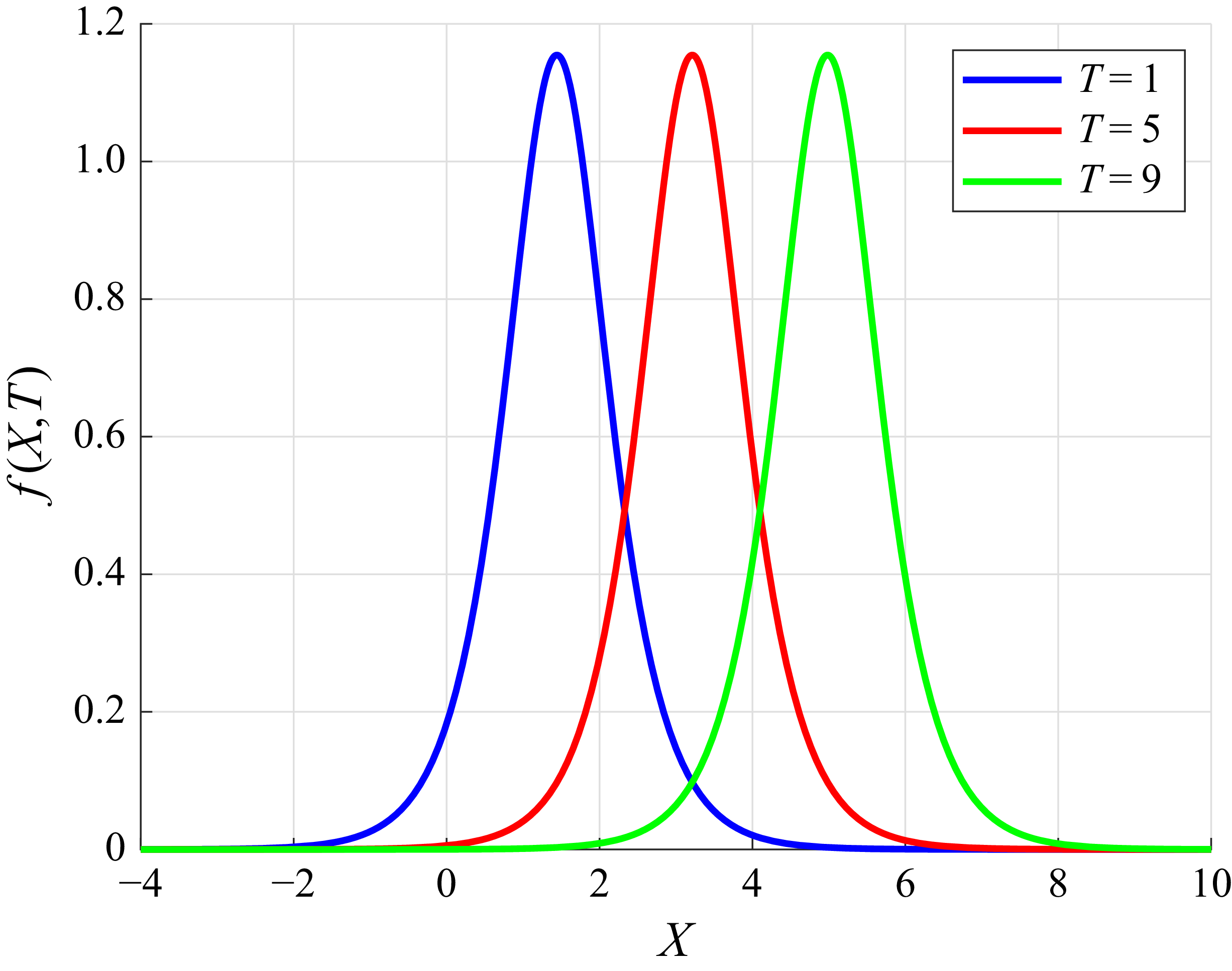
Figure 2 illustrates the one-soliton solutions at time points $T=1,5,9$ . Without loss of generality, parameters are selected as $b_1={\pi }/{2},\ b_3={\pi }/{6},\ k_1=2,\ \eta _1=2,\ \gamma _1={\pi }/{3}$ . As depicted in figure 2, as the value of $T$ increases, the position of the single-soliton solution exhibits a significant translation along the $X$ -axis, while its profile shape remains largely unchanged. This indicates that under ideal conditions, where factors such as dissipation are not taken into account, it exhibits the key characteristic of shape stability during the propagation of solitons.

Figure 2.

One-soliton solution diagrams for different time $T$ values, with $b_1={\pi }/{2},\ b_3={\pi }/{6},\ k_1=2,\ \eta _1=2$ .

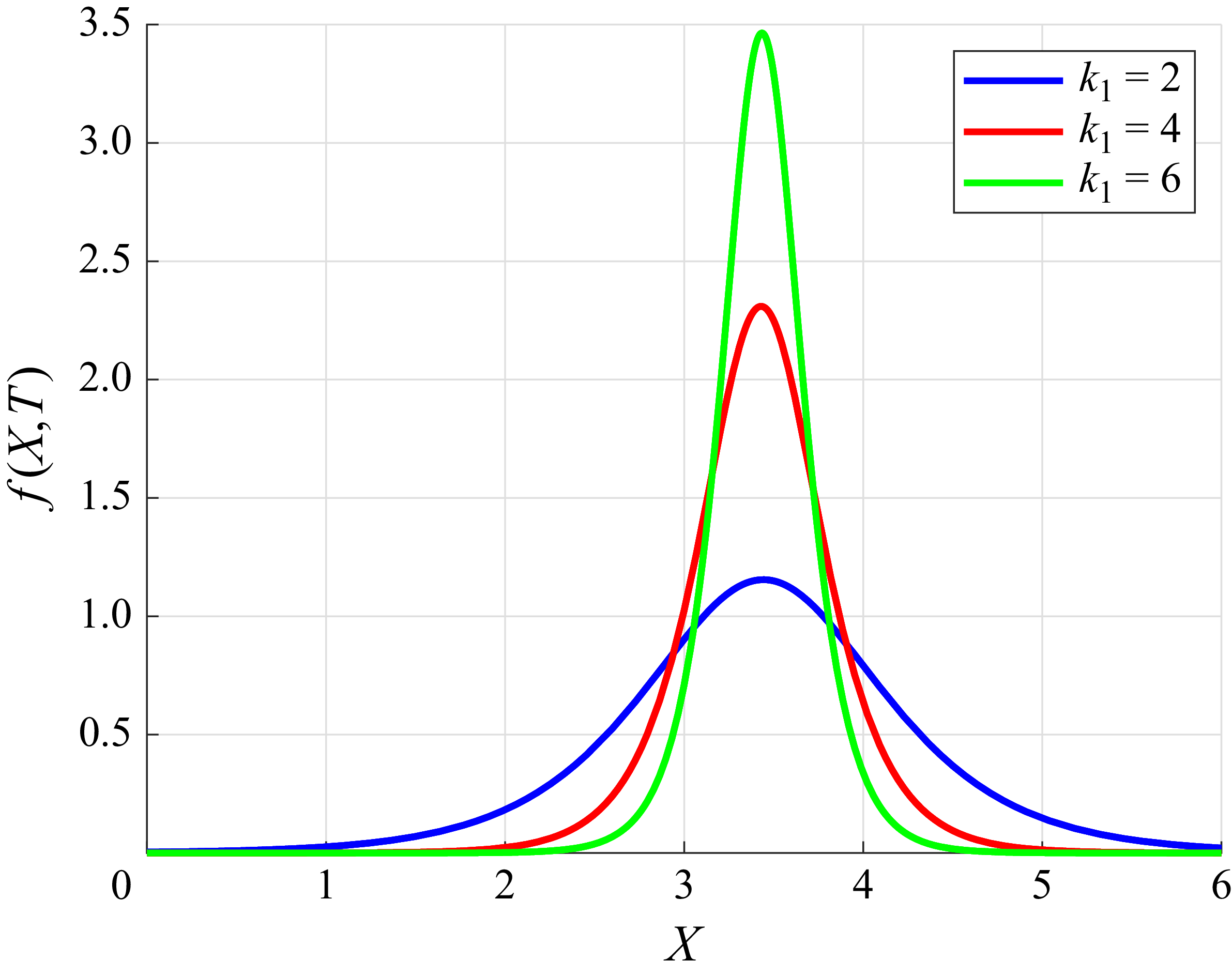
Figure 3 shows the influence of different $k_1=2,4,6$ values on the one-soliton solution with $b_1={\pi }/{2},\ b_3={\pi }/{6},\ T=1,\ \gamma _1={\pi }/{3}$ . From figure 3, it is clearly observed that as the wavenumber $k_1$ increases, the peak amplitude of the single-soliton solution curve exhibits a significant upward trend, while the curve’s profile becomes steeper and sharper.

Figure 3.

One-soliton solution diagrams for different $k_1$ values.

In soliton theory and related physical models, the wavenumber $k_1$ serves as a critical parameter that directly influences the amplitude and morphological characteristics of the single-soliton solution. By comparing the curves corresponding to different values of $k_1$ in figure 3, we can provide intuitive and effective visual data support for further investigating the role of wavenumber in soliton propagation and interaction processes. This analysis contributes to a deeper understanding of the dynamical behaviour of solitons under varying wavenumber conditions.

Next, we compare the soliton solution of the mILW equation with that of the ILW equation, for which we use the soliton solution found in Matsuno (Reference Matsuno1979) using Hirota’s bilinear method as follows:

(4.16) \begin{equation} \begin{aligned} f=\lambda \gamma _1\sin (\gamma _1)\times \left \lbrace \cosh \left [\lambda \gamma _1\left ( X-c_1T-\delta _1\right ) \right ] +\cos \left (\gamma _1 \right ) \right \rbrace ^{-1}. \end{aligned} \end{equation}

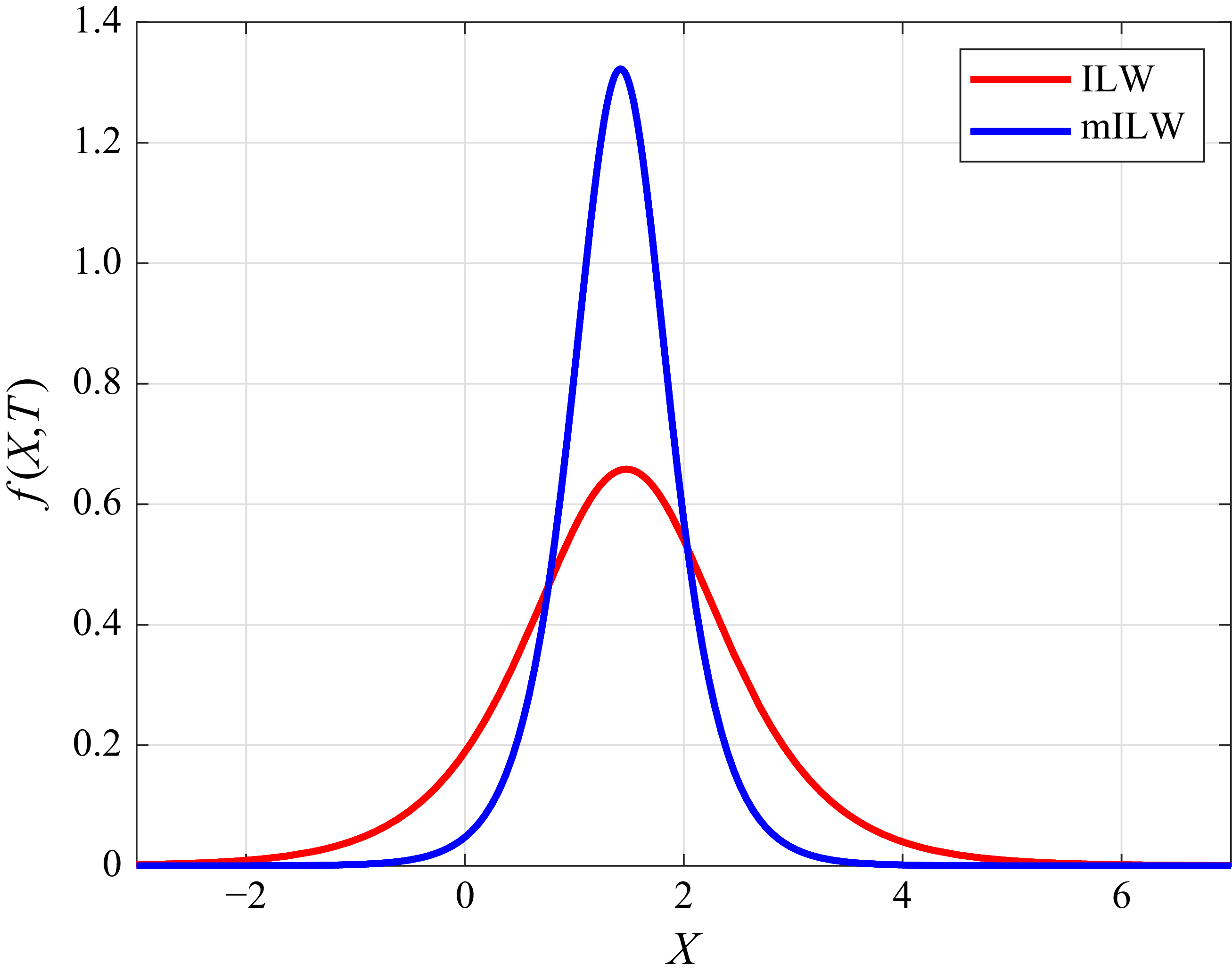
The parameter values are chosen to be $b_1={\pi }/{6},\ b_3={\pi }/{12},\ T=2, \gamma _1={\pi }/{4},\ \eta _1=2$ . As shown in figure 4, it is evident that within the same spatial domain, the peak amplitude of the solution curve for the mILW equation is significantly higher than that for the ILW equation, indicating that the mILW model has a higher amplitude than that of the ILW model. Additionally, the gradient of the mILW solution curve is steeper, suggesting more pronounced spatial variations. This demonstrates that the mILW model exhibits stronger nonlinearity compared to the ILW model.

Figure 4.

Comparison of the solutions of the ILW equation and the mILW equation.

For the two-soliton solution, comparing the coefficients of $\epsilon ^2$ , we have

(4.17) \begin{equation} \epsilon^{2} : \left \lbrace \begin{aligned} &\mathrm{i}\big ( g^{(2)+}-g^{(2)-}\big )_T+\frac {1}{6}b_1\mathrm{i}\big ( g^{(2)+}-g^{(2)-}\big )_{\textit{XXX}}-b_3\big ( g^{(2)+}+g^{(2)-}\big )_{\textit{XX}}\\&\!=-\mathrm{i}\big ( g^{(1)+}_Tg^{(1)-}-g^{(1)+}g^{(1)-}_T\big )b_3\big ( g^{(1)+}_{\textit{XX}}g^{(1)-}-2g^{(1)+}_{X}g^{(1)-}_X+g^{(1)+}g^{(1)-}_{\textit{XX}}\big )\\& \!- \frac {1}{6}b_1\mathrm{i}\big ( g^{(1)+}_{\textit{XX}}g^{(1)-}-g^{(1)+}g^{(1)-}_{\textit{XXX}}-3g^{(1)+}_{\textit{XX}}g^{(1)-}_{X}+3g^{(1)+}_{X}g^{(1)-}_{\textit{XX}}\big ). \end{aligned} \right . \end{equation}

We can truncate (4.10) to $g^{(2)+}(X,T)$ and $g^{(2)-}(X,T)$ :

(4.18) \begin{equation} \begin{aligned} g^-(X,T)=1+\epsilon g^{(1)-}+\epsilon ^2g^{(2)-},\quad g^+(X,T)=1+\epsilon g^{(1)+}+\epsilon ^2g^{(2)+}. \end{aligned} \end{equation}

Taking $g^{(1)-}={\rm e}^{\theta _1+\mathrm{i}\gamma _1}+{\rm e}^{\theta _2+\mathrm{i}\gamma _2 }$ , we find that $g^{(2)-}$ is obtained as

(4.19) \begin{equation} \begin{aligned} g^{(2)-}=A_{12}\,{\rm e}^{\theta _1+\theta _2+\mathrm{i}(\gamma _1+\gamma _2)}, \end{aligned} \end{equation}

with

(4.20) \begin{equation} \begin{aligned} &A_{12}=\\&\frac {2\left (\omega _1-\omega _2\right )\sin \left (\gamma _1-\gamma _2\right )+3b_1\left (k_1-k_2\right )^3\sin \left (\gamma _1-\gamma _2\right )-2b_3\left (k_1-k_2\right )^2\cos \left (\gamma _1-\gamma _2\right )}{2\left (\omega _1+\omega _2\right )\sin \left (\gamma _1+\gamma _2\right )+3b_1\left (k_1+k_2\right )^3\sin \left (\gamma _1+\gamma _2\right )-2b_3\left (k_1+k_2\right )^2\cos \left (\gamma _1+\gamma _2\right )}. \end{aligned} \end{equation}

Substituting (4.19) into (4.10), the two-soliton solution of (2.36) is

(4.21) \begin{equation} \begin{aligned} f=\frac {-2\left ( B_2C_1-B_1C_2\right ) }{B_1^2+B_2^2},\\ \end{aligned} \end{equation}

where

(4.22) \begin{equation} \begin{aligned} &B_1=1+\textrm{e}^{\theta _1}\cos {\gamma _1}+\textrm{e}^{\theta _2}\cos {\gamma _2}+A_{12}\,\textrm{e}^{\theta _1+\theta _2}\cos {\gamma _1+\gamma _2},\\ &B_2=\textrm{e}^{\theta _1}\sin {\gamma _1}+\textrm{e}^{\theta _2}\sin {\gamma _2}+A_{12}\,\textrm{e}^{\theta _1+\theta _2}\sin {\gamma _1+\gamma _2},\\ &C_1=k_1\,\textrm{e}^{\theta _1}\cos {\gamma _1}+k_2\,\textrm{e}^{\theta _2}\cos {\gamma _2}+A_{12}\left (k_1+k_2 \right )\, \textrm{e}^{\theta _1+\theta _2}\cos {\gamma _1+\gamma _2},\\ &C_2=k_1\,\textrm{e}^{\theta _1}\sin {\gamma _1}+k_2\,\textrm{e}^{\theta _2}\sin {\gamma _2}+A_{12}\left (k_1+k_2 \right )\, \textrm{e}^{\theta _1+\theta _2}\sin {\gamma _1+\gamma _2}.\\ \end{aligned} \end{equation}

Similarly, one can continue to calculate the three-soliton solution and four-soliton solution of the equation. Here, we will not elaborate further on this.

5. Interaction between solitary waves

In § 4, we set $b_1=6b_2$ . To justify the condition $b_1=6b_2$ adopted in the model, we conducted a systematic parameter optimisation based on realistic oceanic stratification. Specifically, we considered a two-layer density structure in which the upper layer ( $h\geqslant {z}\gt {0}$ ) exhibits a vertical variation in density, while the lower layer ( ${0}\geqslant z\geqslant {-H}$ ) maintains a constant background density $\rho _0(0)$ . Here, $z=h$ corresponds to the ocean surface. A commonly used $\tanh$ -type density profile in oceanography is adopted, and its explicit form is given as

(5.1) \begin{equation} \begin{aligned} \rho _0(z)=\bar {\rho }-\Delta \rho \tanh \left ( \frac {z-z_0}{d}\right )\! ,\\ \end{aligned} \end{equation}

where $\rho _0(z)$ denotes the density as a function of depth $z$ , $\bar {\rho }$ is the mean density of seawater, typically taken as 1025 kg m⁻ $^{3}$ , and $\Delta \rho$ represents the density contrast. The parameter $z_0$ denotes the centre depth of the pycnocline, while $d$ controls the thickness and sharpness of the stratification transition.

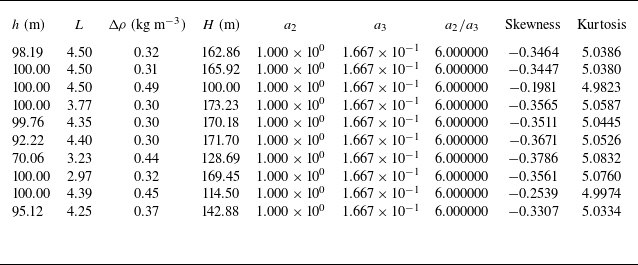
From (2.36), we can observe that $b_1=a_2/a_1$ and $b_2=a_3/a_1$ . To simplify the computation, it suffices to determine the parameter sets for which $b_1/b_2=a_2/a_3=6$ . We utilised both grid scanning and global optimisation (particle swarm) techniques, and successfully identified multiple physically reasonable parameter sets for which $a_2/a_3=6$ is achieved with high precision (to within $10^{-6}$ relative error). Table 1 shows the ten parameter sets $a_2/a_3=6$ .

Table 1.

Top ten stratification parameter sets for which $a_2/a_3 \approx 6$ .

Notably, these optimal stratifications are consistent with observed oceanic conditions (e.g. upper-layer thickness 50–100 m, density differences 0.3–0.5 $\rm kg\ m^-{^3}$ ). These results demonstrate that the assumption $a_2/a_3=6$ can be consistently realised within the framework of physically relevant stratification. Thus the use of this value in the theoretical formulation is justified, and the soliton solutions and their interaction properties discussed are based on realistic and representative oceanic environments.

Moreover, for each optimal parameter set, the computed skewness and kurtosis of the vertical velocity field provide further physical insight into the wave asymmetry and localisation induced by stratification. Specifically, we observe that the skewness values are consistently negative (approximately from $-0.20$ to $-0.38$ ), indicating an asymmetric wave structure characterised by enhanced downward motion beneath the pycnocline – a hallmark of nonlinear internal waves in oceanic settings. The kurtosis values range from approximately 4.98 to 5.08, significantly exceeding the Gaussian baseline 3, confirming that the wave energy is sharply concentrated around the wave crest, with heavy-tailed vertical distribution.

Importantly, both skewness and kurtosis exhibit sensitivity to stratification parameters. A larger density jump $\Delta \rho$ or sharper pycnocline (smaller $L$ ) enhances the nonlinearity of the system, which in turn leads to stronger asymmetry (more negative skewness) and sharper wave localisation (higher kurtosis). These statistical indicators thus reflect and reinforce the conclusion that the selected parameter regime supports stronger nonlinear solitary waves, and validate the capacity of the mILW model to capture essential dynamical features observed in realistic oceanic environments.

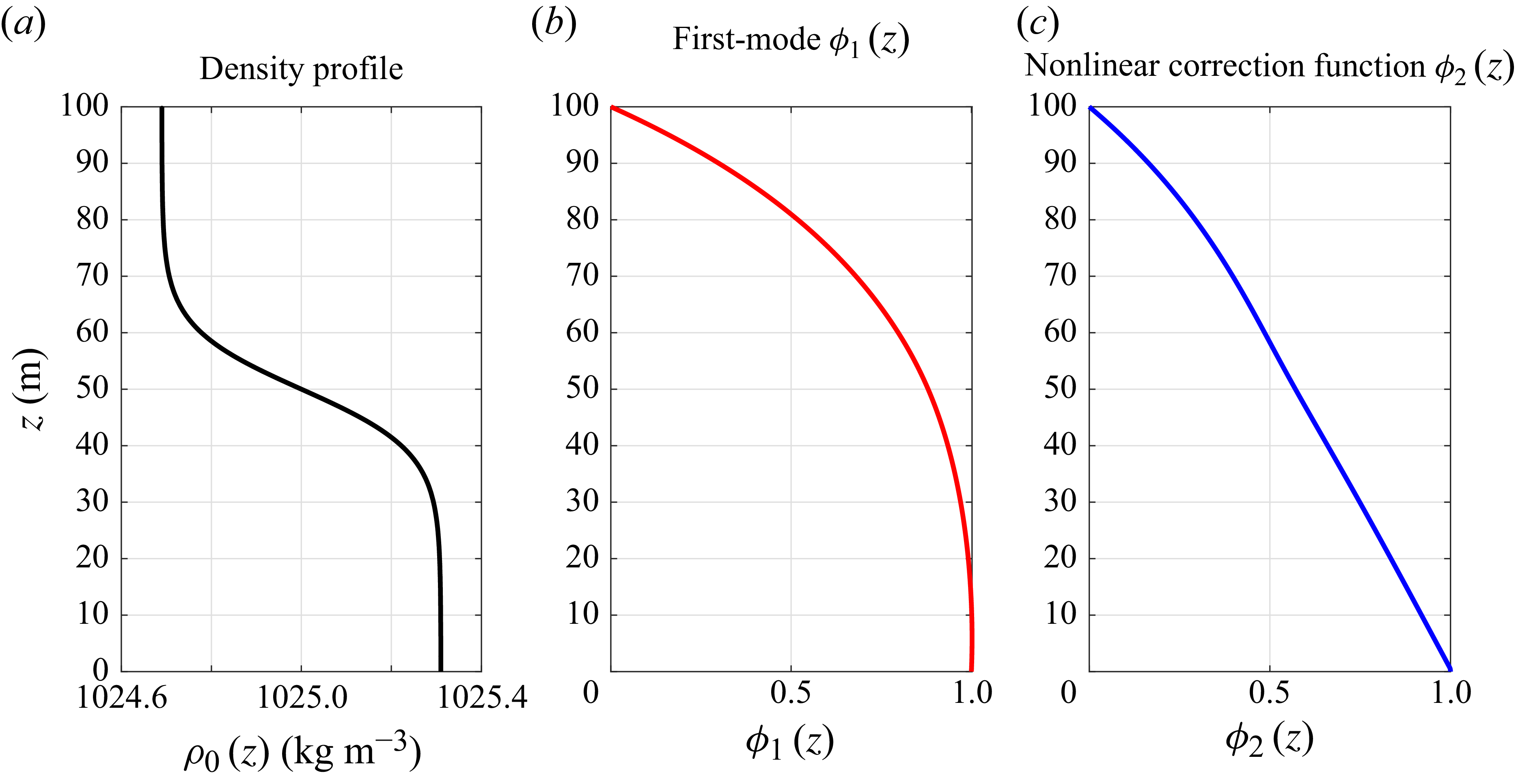
To further clarify the role of the density structure in shaping the modal dynamics and nonlinear wave behaviour, we include the computed vertical structure functions and resulting vertical velocity field in figures 5 and 6, with $h=100$ , $L=4.5$ , $\Delta \rho =0.31$ . Figure 5 illustrates the stratification profile and the corresponding vertical modal structures derived from the background density field. Figure 5(a) shows the background density $\rho _0(z)$ , defined by a hyperbolic tangent function that creates a pronounced pycnocline centred at the interface $z=0$ , which separates the homogeneous lower layer from the stratified upper layer. The vertical coordinate $z\in [0,h]$ is oriented upwards, with $z=h$ at the surface.

Figure 5.

Density profile and vertical structure of modal functions.

Figure 6.

Vertical structure of velocity components $w_1$ , $w_2$ and total field $w$ .

Figure 5(b) displays the first-mode structure function $\phi _1(z)$ , obtained by solving the Sturm–Liouville-type eigenvalue problem derived in § 2. In this study, we adopt a fixed boundary normalisation for the first-mode structure function $\phi _1(z)$ , such that $\phi _1(h)=0$ at the surface, and $\phi _1(0)=1$ at the bottom of the upper fluid. This choice aligns with the theoretical framework, and ensures consistent comparison across different stratification profiles. The resulting modal function is strictly confined within the interval $[0,1]$ , facilitating the interpretation of vertical structure and its influence on nonlinear wave evolution. As expected, $\phi _1(z)$ increases monotonically from the surface to the bottom, representing the primary mode that governs the vertical structure of ISWs.

Figure 5(c) shows the nonlinear correction function $\phi _2(z)$ , which emerges from the second-order perturbation expansion and accounts for nonlinear modifications to the wave field. Notably, the function $\phi _2(z)$ exhibits a monotonic decrease from the bottom to the surface, indicating that the nonlinear contributions are more prominent in the lower part of the stratified region. This structure introduces asymmetry into the vertical distribution of wave-induced velocity and density perturbations. This contributes to bottom intensification and asymmetrical wave profiles in strongly stratified fluids.

Figure 6 presents the vertical structure of the ISW’s vertical velocity field $w(X,z,T)$ , decomposed into its leading-order and second-order components derived from nonlinear theory. Figure 6(a) shows the first-order velocity component $w_1(X,z,T)=-\phi _1(z)\,f_X$ , which captures the dominant structure of the wave. The velocity exhibits a symmetric dipole pattern centred around the wave crest near $X=-10$ m, with upward motion on one side, and downward motion on the other. This structure is vertically confined and aligned with the interface, diminishing towards the surface due to the boundary condition $\phi _1(h)=0$ , and reflects the classical modal shape typical of first-mode internal waves.

In contrast, figure 6(b) displays the second-order correction $w_2(X,z,T)=-\phi _2(z)\,ff_X$ , which introduces clear asymmetry into the wave-induced vertical motion. The spatial pattern is notably intensified towards the lower portion of the upper layer, consistent with the shape of the second-order modal function $\phi _2(z)$ , which peaks near the interface and decays upwards. This asymmetry is a hallmark of nonlinear effects in stratified fluids, where nonlinear steepening preferentially enhances velocities beneath the wave core, and suppresses upward return flow above.

Figure 6(c) combines the two contributions into the total vertical velocity field, constructed as $w=\epsilon w_1+\epsilon ^{({3}/{2})} w_2$ , with a small nonlinearity parameter $\epsilon =0.1$ . The result is a realistic and asymmetrical wave profile that deviates from the $w_1$ prediction. The composite field retains the dipole character of $w_1$ , but with skewed amplitude distribution and bottom-intensified structure, underscoring the significance of the second-order term. These features are consistent with theoretical expectations for ISWs in stratified upper-ocean environments, and confirm the effectiveness of the mILW model in capturing both dispersive and nonlinear effects in internal wave propagation.

Building upon prior research (Yu & Song Reference Yu and Song2024), which explored the interaction of two solitary waves in the modified BO equation, this study employs a similar methodology to examine the oblique interaction of solitons within the mILW equation. Utilising the soliton solution from § 4, the interaction of two solitary waves with the same amplitude is investigated next, and the effects of the parameters $k_1$ and $\eta _1$ on the interaction of the solitary waves are investigated by the control variable method.

As shown in figure 7, two solitary waves with the same amplitude are placed symmetrically along the line $X=0$ . This can be expressed by the equation

(5.2) \begin{equation} \begin{aligned} f=\frac {2k_1\,\textrm{e}^{k_1X+\omega _1T}\sin {\gamma _1}}{1+\textrm{e}^{2(k_1X+\omega _1T)}+2\,\textrm{e}^{k_1X+\omega _1T}\cos {\gamma _1}}+\frac {2k_1\,\textrm{e}^{-k_1X+\omega _1T}\sin {\gamma _1}}{1+\textrm{e}^{2(-k_1X+\omega _1T)}+2\,\textrm{e}^{-k_1X+\omega _1T}\cos {\gamma _1}}. \end{aligned} \end{equation}

The central axis effectively functions as a virtual rigid boundary. This interaction replicates the reflection pattern observed when an incident solitary wave encounters a vertical rigid wall. The highlighted region corresponds to the developing Mach stem. Under idealised, dissipation-free conditions, the collision of two solitary waves with identical amplitudes exhibits dynamics analogous to wall reflection. During this process, a reflected wave emerges and evolves into solitons matching the incident wave characteristics. Initial wave overlap transforms into an amplified solitary wave structure extending along the $X$ direction, identified as the Mach stem.

Figure 7.

Illustration of the solution $f(X,T)$ with $b_1={\pi }/{6},\ b_3={\pi }/{12},\ k_1=1.2,\ \eta _1=0.1$ : (a) front view, (b) side view, (c) vertical view.

The Mach stem undergoes distinct developmental phases: initiation during wave interaction, followed by sustained growth that eventually stabilises after finite time. This characteristic evolution confirms a well-defined Mach-type reflection process.

As shown in figure 8, this type can reflect the interaction patterns in the real ocean, and was captured by the RADARSAT-1 satellite in South African waters in 1990 (Global Ocean Associates 2004). Zheng et al. (Reference Zheng, Klemas and Yan1997) analysed satellite imagery, and reported that both groups of ISWs propagate shorewards. When these wave packets intersect, complex nonlinear interactions are observed.

Figure 8.

The interaction of oceanic ISWs (astronaut photograph STS036–082-76 acquired on 1 March 1990 at 1254 UTC), from Global Ocean Associates 2004.

As shown in figure 9(a,b,d,e), if the wavenumber $k_1$ is kept constant and only the initial phase $\eta _1$ is changed, then the interaction time of the two solitary waves and the shape of the stem remain unchanged, but with the increase of $\eta _1$ , the interaction time of the two solitary waves is delayed. Keeping the value of the initial phase $\eta _1$ constant and changing the value of the wavenumber $k_1$ , as shown in figure 9(a,c,d,f), the time taken for the two solitary waves to interact becomes shorter, and the amplitude of the stem increases but their widths become narrower as the wavenumber $k$ increases.

Figure 9.

The interaction of solitary waves with $b_1={\pi }/{6},\ b_3={\pi }/{12}$ .