Introduction
Cryptography is a means to shift security concerns for context-rich data to randomized data (cryptographic keys).[Reference Smart1, Reference Stöcker and Samid2] It is by laying hands on these keys that data is compromised. The strategic counter-measure therefore is to secure this random data. We propose to do so with a “Rock of Randomness.”
The underlying idea for the rock is its physicality: it carries its information content implicitly rather than explicitly, and hence this, so held, information requires the presence of this physicality, this rock. Alas, one would argue, if the rock can release its information, even if bit by bit, then it can be exhaustively queried and the answers can be properly tabulated to create an equivalent oracle. This premise is of course true in principle. However, a physical device, even a small one, can be made to contain so much information that it renders its explicit mirror to be infeasible on several levels: (i) on sheer ability to log all these very many bits, (ii) on the time it takes to copy the implicit information into explicit tables, (iii) on the conditions, the equipment and facilities needed to accomplish this task.
Copying the data is one way to compromise it, and duplicating the contraption, the rock, is another. The random rock is designed to withstand duplication based on possession only (without the manufacturing plan).
In summary, we have here a physical element that contains shareable randomness in an implicit form that requires its presence. The device, the randomness rock, effectively resists duplication, and contains too much information that resists “wholesale” queries, rendering their extraction infeasible. These features upgrade the security level associated with such shared randomness. One just needs to keep these rocks in a secure physical confine, and thereby its content is protected from attack.
Principles of operation
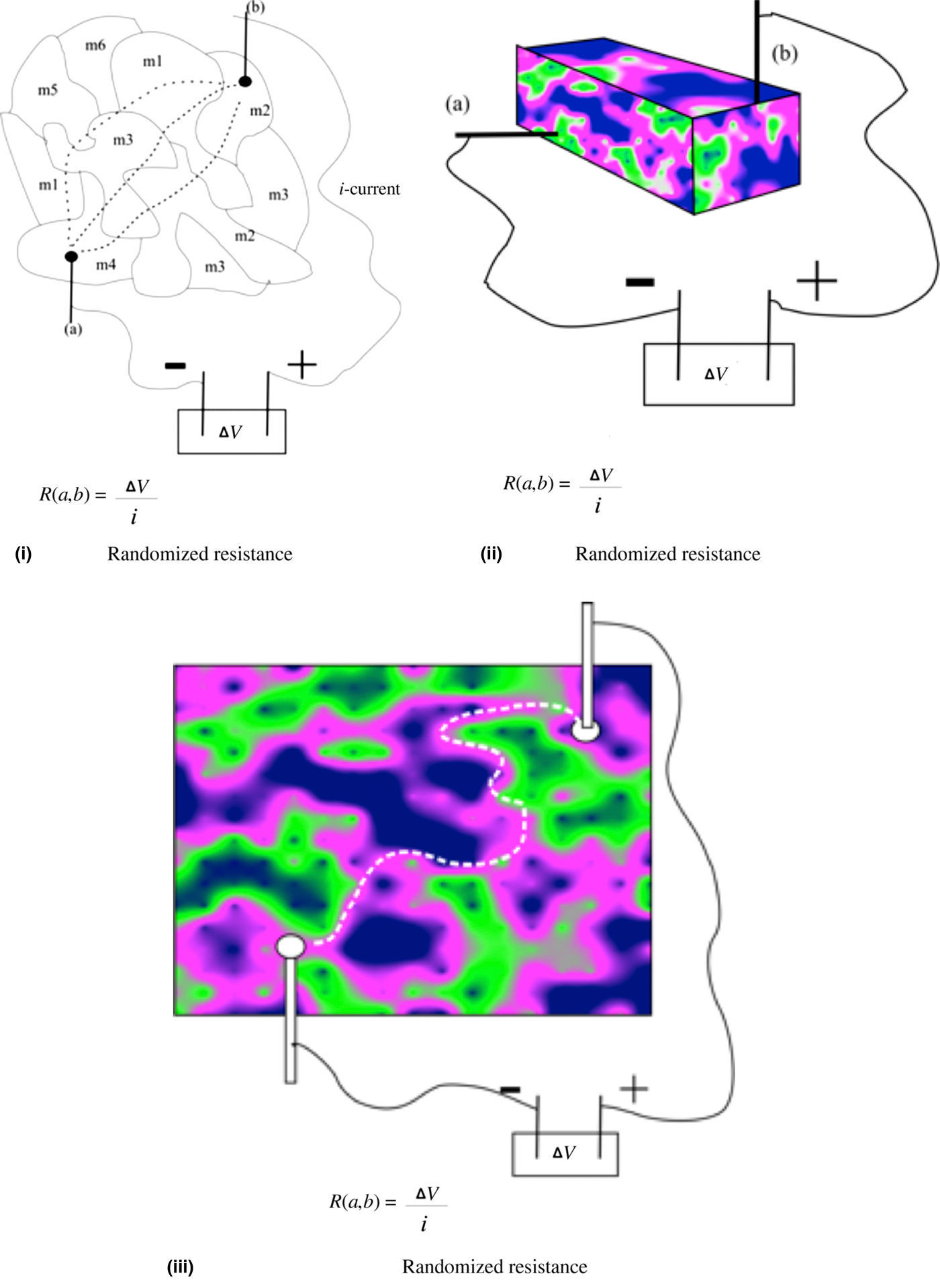
The random rock is comprised of a mixture of variant-electrical conductivity materials, such that the electrical resistance measured between two arbitrary points on the surface of the rock depends on (i) the electrical conductivity of the comprising materials, on their relative geometry within the rock, and on any electrical interaction across shared surfaces. Two or more sufficiently identical rocks will log the same electrical resistance between the very same points on each respective rock (Fig. 1).
Randomized resistance: three views of the randomized construction of the “rock” such that the measured resistance between two arbitrary points will also be randomized. (i) Depicts multi pathways for current flow; (ii) depicts the brick (rock) structure in 3D; (iii) depicts drilled ports option (increased variety).
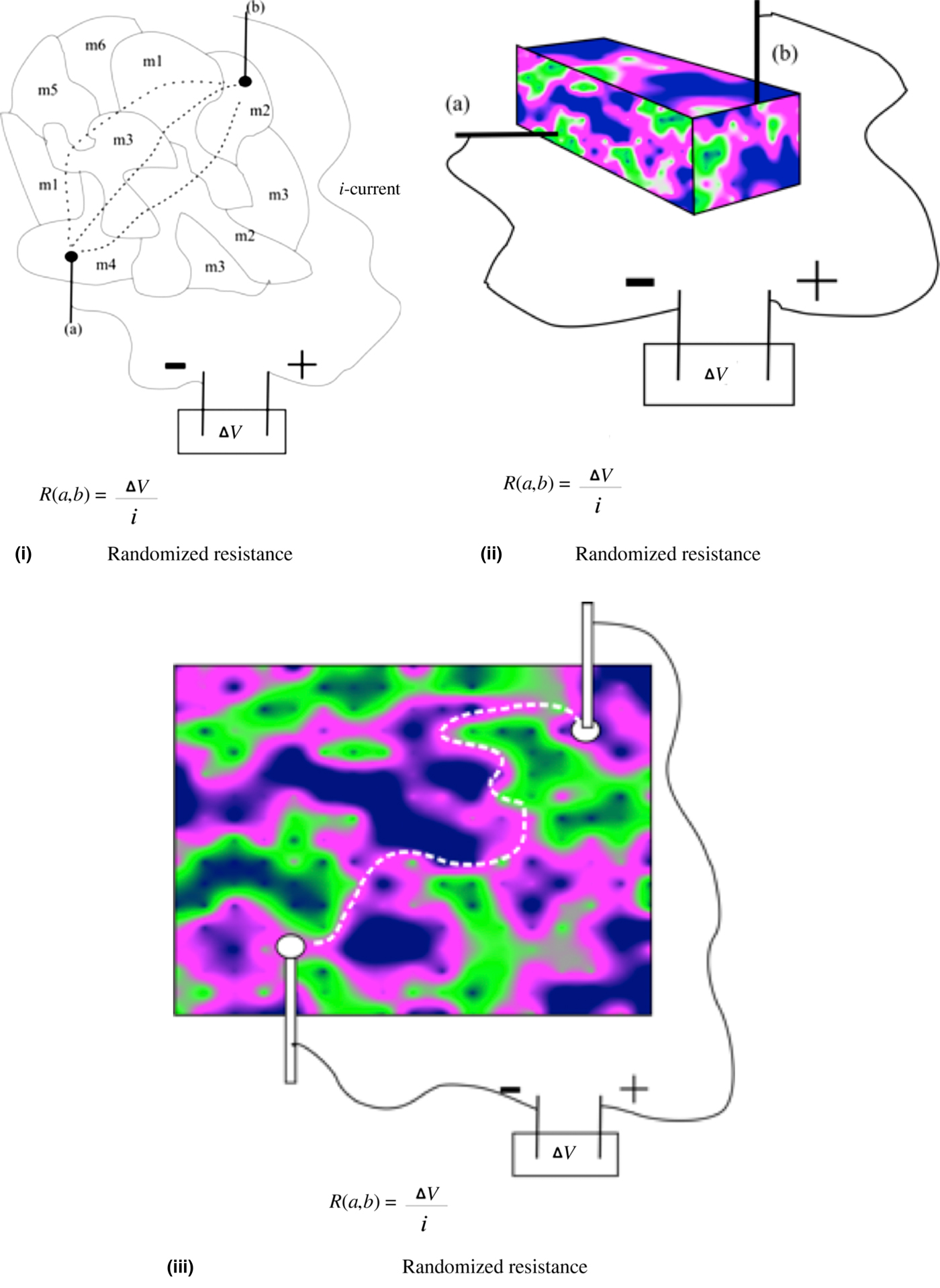
Using modern technology, it is possible to construct any desired count, (C), of sufficiently exact duplicates of such a rock where the relative geometry of the comprising materials will be properly randomized. The C rocks may then be distributed to C communicating parties. Each party then will be able to pull shared randomness from the rock by indicating in the open the location of the two points between which to measure the resistance. Each of the C communicating parties will be measuring the resistance on its own rock, and the result of this measurement will be the shared randomness among the C communicating parties. Why randomness? Because the original geometric layout of the comprising materials was carried out via a proper random number generator (RNG), and therefore the reading of the resistance between the two designated points will also be random, and a secret shared between the rock holders, hidden from anybody else.
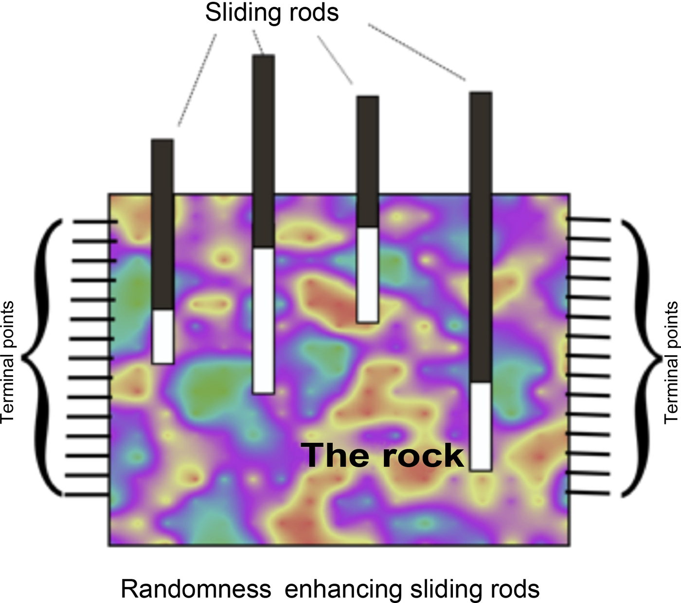
We further propose to upgrade the rock with “sliding conductor rods.” In order to increase the amount of randomness that is housed by the rock, we propose to drill holes inside it, and fit disruptive rods that would slide into these drilled holes in a variable measure. The rods’ position will span from remaining outside the holes to sliding completely inside the holes. The sliding status of these rods will affect the reading of the resistance between any two arbitrary points. While the randomness that generated the composition of the rock is shared, secret, and hidden, the status of the sliding rods can be also determined randomly by an initiating party (among the C communicating parties), and shared openly, so that each party will know how to set the position of the rods to get the same resistance reading as the other parties.
The sliding rods enhancement will frustrate any adversary trying to take a measure of the resistance between all possible pairs of points. There will be so many more combinations due to the large position variability of the rods, that pre-mapping will not be feasible.
We now continue with (i) mathematical analysis, (ii) manufacturing technology, (iii) applications, (iv) security analysis, and (v) future outlook.
Mathematical analysis
The rock is a randomized composition of its comprising materials. Its boundary is the surface where terminal points are marked.
At the operational level, the random rock will function like an oracle. Two terminal points will be identified, (i,j), and a resistance reading, r(i,j) will be measured over the rock. The reading will have to be mapped into an integer ρ(r), and ρ will be the shared secret, or part thereof. Let us identify n terminal spots on the rock. This defines n(n−1)/2 pairs, which defines n(n−1)/2 readings, r(i,j). This analysis refers to the fixed rock construction without the sliding rods. Among the n(n−1)/2 readings, there is a highest reading r h, and the lowest reading r l. Based on the accuracy of the reading device, the fidelity of the duplications of the rock, and the environmental impact, one can identify an “interval of fluctuation” δr, which reflects the expected difference in actual readings between the various parties, each holding a different copy of the same rock at a different location. Based on δr, one can identify an “interval of accuracy” (IOA), as some multiplier of δr (IOA = k*δr) as an interval of resistance readings that will be comfortably larger than the error span of readings among the communicating parties. The parties will then agree on a reference reading r m, which should be close to the middle point between r l and r h: r m ~0.5(r h−r l). Once r m is agreed upon, then it may serve as an anchor to define IOA intervals higher and lower than r m. Once so, then any reading of resistance between r l and r h will fit into one IOA interval. The intervals may be enumerated to facilitate the translation of r(i,j) to ρ(i,j) = −q, −(q−1), −(q−2),… −1, 1, 2,….q. where 2q ⩽ (r h−r l)/IOA.
An arbitrary reading of resistance, r, will be found to be: r m + (k−1) × IOA < r < r m + k × IOA, and translated to ρ(r) = k, or found to be: r m−(k + 1) × IOA < r < r m−k × IOA, and translated to ρ(r) = −k.
Dynamics: Any party among the c communicating parties will randomly choose two terminal points, (i,j), and measure the electrical resistance between them, r(i,j). Based on the shared values of r m and IOA, the measuring party will check if the reading r(i,j) is too close to an “interval flip point” (IFP). IFP is defined as a reading of resistance, r, such that a reading r′ < IFP translate to different interval than a reading r′′ > IFP: ρ(r′) ≠ ρ(r′′). In other words, an IFP value is the value that serves as the higher boundary for one IOA interval and the lower boundary for another IOA interval. If |r(i,j)−IFP| ⩽ δr, then there is risk that the reading errors among the communicating parties will result in one or some communicating parties translating the r(i,j) to an integer ρ(i,j) different from the rest. Therefore, if the reading r(i,j) is too close to an IFP, this reading should be discarded, and the measuring party should randomly choose a different pair (i′,j′), and again discard it if the corresponding reading r(i′,j′) is too close to an IFP, and repeat choosing pairs of terminals until a reading comes forth that is not too close to an IFP. The parties may agree on a measure of “too close,” namely on a value of k′ such that: |r(i,j)−IFP| > k′r.
Following the above procedure the parties will be able each to initiate a sequence that would generate a shared secret, integer ρ, which can be used as such, or be part of a larger secret built up by repeating this procedure as many times as desired.
For this contraption to work it is necessary that the interval (r h−r l) will be large enough (the measuring span), and it is further necessary that an adversary who knows everything about this procedure, except that she does not possess the rock itself, will not be able to deduce or to learn anything consequential about the measured value r(i,j).
We shall assume that the adversary knows the values of r h and r l (the limits awareness assumption). We further assume that the adversary knows, or has a good guess of δr, and hence can come up with a good guess of the IOA. We further assume that the adversary discovers the value of the reference reading, r m. With all that knowledge, the adversary can readily translate a reading r(i,j) to its corresponding interval ρ(i,j).
For the contraption to project maximum security, it is necessary that for each pair of terminal points (i,j), the chance for the corresponding integer reading ρ(i,j) will be 1/2q. In other words, every reading among the 2q possible values will have the same likelihood to be the reading associated with an arbitrary pair (i,j).
This equi-distribution will have to be provided, or sufficiently approximated for by the randomness rock construction to function as intended.
Rock construction
The randomness rock is built with c distinct comprising materials. M 1, M 2,…M c. They each have a distinct electrical conductivity index σ 1, σ 2,…σ c, such that σ i ≠ σ j for every i ≠ j. The choice of the participating materials will be such that no two conductivity indices will be too close to each other: |σ i−σ j|min > γ, where γ is a boundary limit of closeness; i,j = 1, 2, …c; i ≠ j.
The measured conductivity (or resistance) between any two points on the rock depends on the distribution of the c comprising materials, as they spread out between the two terminal points. This distribution will be determined via a high-quality RNG that will guide a manufacturing procedure to manufacture sufficiently identical t rocks. The randomness of the distribution of the c materials will be translated into randomness of the resistance reading between any two arbitrary points on the rock.
We analyze below the rock composition randomness requirements.
Rock composition randomness requirements
Let us first review the boundary conditions. Let the participating materials be organized such that σ 1 > σ 2 > …σ c, namely organized in declining conductivity. Let us further agree on some naming order to mark the n terminal points: i,j = 1, 2,….n
If the rock is comprised of material k only then the resistance r(i,j) will be dependent only on the geometry of the rock between points i and j. Furthermore, there would be a close proximity between r(i,j) and r(i + η, j + η), where η = +1, +2, + 3, −1, −2, −3. Namely by moving one terminal to a neighboring terminal point, the new reading will be close to the former one—randomness lost.
This loss of randomness will apply no matter which of the c materials has been chosen. We may be cautious and assume that the external geometry of the rock (its dimension) is known to the adversary and hence she could build a replica of the rock, and if she knows the code for identifying the terminal points, then she could arrive at the right measurement and uncover our secret.
Let us now analyze the opposite case, where all c materials are being thoroughly mixed when constructing the rock. In this case, one again achieves homogeneity, and the reading r(i,j) will be dependent only on the geometry, the positions, of i and j versus the geometry of the rock, and again the adversary could build a replica of the rock, assuming she knows all the materials we selected M 1, M 2,…M c.
We conclude then that “no mixing” and “thorough mixing” are inappropriate for our aim. What is needed is incomplete mixing to generate sufficient randomness in the set of measurements.
Incomplete mixing
To meet the challenge of incomplete mixing, we shall first entertain the challenge of optimal configuration (mixing). Given arbitrary, but well-defined external shape of the rock, and given the positions of the n terminal points on its surface, and also given the set of c participating materials, M 1, M 2,…M c, with known conductivity indices σ 1, σ 2,…σ c, one would define an exact criteria for rating efficacy of different mixing configurations. The Shannon entropy[Reference Shannon3, Reference Camesasca, Kaufman and Manas-Zloczower4] can be used here, or alternatively, as follows: for a given mixing configuration, and for each proximity distance |i−j| = d, let us build a histogram h(x), where x reflect the ρ value, hence 1 ⩽ x ⩽ 2q, and h(x) reflects the number of pairs for which the measured value for ρ is x. There are n(n−1)/2 such pairs hence:
 $$\mathop \sum \limits_{d = 1}^{d = n-1} \mathop \sum \limits_{x = 1}^{x = 2q} h(x,\,d) = \displaystyle{{n(n-1)} \over 2}.$$
One could use standard regressions of these histograms relative to a horizontal line, and use the standard deviation from such a line as the metric for the quality of distribution of resistance values. The ideal case is when for each pair of terminal points (i,j), the chance for any value of ρ is 1/2q: Pr(ρ)i,j = 1/2q for i,j = 1, 2,… n.
While a pure mathematical calculation appears quite intractable, this challenge lends itself easily toward a standard optimization; whether based on mathematical modeling or based on actual experimentation.
If there is one such optimal configuration, then it should NOT be used by the rock builder. The reason is that the adversary, aware of the dimensions of the rock, will be able to also arrive at that optimal configuration and use it to uncover the secret. This leads to a strange situation—the mixing which leads to optimal distribution of the measured values—optimal in the sense that it would be most intractable for an adversary to guess—is in fact a bad choice because it is based on mathematical insight which the adversary is assumed to possess.
There is a distinct possibility that there will be more than one such configuration where the distribution is optimal. In that case, it will be a bit more challenging for the adversary to go through all these options, but no prudent rock builder will use any of these mathematically optimal configurations.
We have in summary a situation where the two boundary states (no mixing and full mixing) are bad choices, but also the mathematically optimal mixing is a bad choice; and hence we are looking for suboptimal cases that are numerous enough to be sufficiently intractable for discovery by an adversary.
On further thought, the mathematical complexity of resolving this challenge of optimal mixing is the ground argument for the efficacy of the rock. It is to be constructed in some well-randomized fashion, which cannot easily enough be modeled mathematically. It would also lead one to an experimental approach.
Experimental configuration
The experimental configuration strategy will set up some r mixing configurations: z 1, z 2,… z r, and for each configuration, one will measure randomly w pairs selected from the n(n−1)/2 possible pairs. These w measurements will build a histogram h(x), where Σh(x) = w for x = 1, 2,… 2q, and the r histograms will be evaluated as to how flat they are. The “flatness” of these histograms (measured by standard deviation off a horizontal line) will be taken as the metric of the utility of the z-configurations represented by the histogram: u 1, u 2,…u r. The set z 1,…z r, and u 1,…u r will be the basis of optimization where the high utility configurations will be a basis for a Monte Carlo optimization in their mathematical neighborhood. After several rounds of such optimization, the rock builder will establish a procedure to set up a high utility mixing configuration. This configuration style will be implemented with significant randomized input to make the actual reading of the rock, substantially random.
Ahead we will explore plausible such mixing configuration styles.
Mixing configuration styles
We define a randomness rock configuration style as a procedure that determines a mixing state of selected c participating materials with known electrical conductivity indices. We further define two categories of mixing configuration styles: (i) entropic mixing and (ii) pre-blocked mixing. The former calls for partial mixing of the participating materials, such that they do not reach a homogenous state, and the latter is based on setting up blocks in which a single participating material will be filled per block. The two categories are analyzed ahead. The procedure will be comprised of arbitrary design parameters combined with randomized input.
Entropic mixing
Entropic mixing[Reference Camesasca, Kaufman and Manas-Zloczower4–Reference Samid6] is a mixing process of some c ingredients such that the level of mixing is (i) well defined and (ii) operationally controlled. A perfect mix of some c ingredients is one where for very small units of volume, each of the c components will be present in amounts reflective of its relative ratio. An imperfect mix is where many quite large units of volume where the mix is present have only some, not all, of the mixed ingredients.
There are several mathematical methods to quantify the degree of imperfect mixing. One of them is the symmetry-based randomness definition (Samid 2017), which rates any partial (imperfect) mix of c components as to the degree of randomness (perfect mixing) associated with them.
For an entropic mixing to be practical, it is necessary to be in possession of a mixing apparatus where one could input a desired degree of mixing, and have the mixture come out with that degree in a uniform way. Using this method, the rock builder could decide on an optimum and effective degree of mixing of the c participating materials, and then generate such a mixture, which will then have to be copied and duplicated. It is a duplication that keeps this method in a disfavored light. However, for unshared randomness, this aspect is moot, and the entropic mixing is very effective.
Pre-blocked mixing
Pre-locked mixing can take place in two ways: (i) fixed geometry blocks, and (ii) randomized geometry blocks. The first category amounts to establishing blocks, zones inside the rock, and then allowing a randomized selection to select which participating material will be filled into each block. The second category will allow a randomized selection of the boundaries of each block, and then randomized filling.
Terminal construction
The rock contraption will use a conversion table to hide the physical proximity of terminals from the query presenter, but this table has to be assumed as compromised, and hence it is important to minimize the information leak due to knowledge of physical proximity of terminals. The idea being that if one shifts a terminal physically to an adjacent terminal then the reading will be quite similar. Let the n terminals be listed by physical proximity: t 1, t 2,…t n. Namely, the on the rock physical distance between t i and t j is roughly proportional to |i−j|: d ij ~ α × |i−j| (α-coefficient of proportionality). In that case, knowledge of the resistance reading r ik for i and k, two arbitrary terminal points, will decrease the entropy of the unknown reading of r jk, for small values of |i−j||. It is this information leakage that one tries to prevent.
We describe two methods for that purpose that may be used independently or together: (i) terminal blocks, (ii) variable depth pin (VDP).
Blocks: one would surround each terminal with a block to be filled by one of the c comprising materials of the rock. The material choices for adjacent terminals will be such that their conductivity indices are as different as possible.
This defines a clear mathematical challenge. Let (i,k) be two arbitrary terminal points on the rock. Let j = −L, −(L−1),…−1, 1, 2,… L, where L is an arbitrary small number, say L = 4. Let an attacker be aware of all the resistance reading: r [(i + j),k], for all values of j. That attacker will now try to estimate the resistance value r(i,k). The extent that such an estimate is carried out with no more credibility than without the knowledge of the r [(i + j),k] is the extent to which the adjacency information does not leak. Given an established estimation procedure, a given adjunct situation, and c conductivity values, there exists a mathematical solution to minimize the adjacency leakage. It applies for rocks comprised of semi-conductors.
Variable depth pins: Every terminal point i may be extended with a disruptive pin to a randomly variable depth, d i. This will render the distance gap between terminal point i and terminal point i + 1, g(i,i + 1), to be proportional to the gap between d i and d i+1: g(i,i + 1) = α × |d i−d i+1|, where α is a proportionality coefficient. The gap will blur the proximity relationship between the terminals, and will make it more difficult to guess resistance based on neighboring readings.
The pin heads will have to stay mutually apart, and remain inside the confines of the rock. Using the VDP will impact the shape and form of the rock itself.
Conductivity selection
The greater the variety in the conductivity indices, the larger the randomized reading from any pair of terminals. This is easy to show. In the extreme case where all conductivity indices are the same: σ 1 = σ 2 = … = σ t, then by replacing all occurrences of material i in the rock with material j (i ≠ j) there will be no change in the readings of the resistance between any pair of points on the rock; and hence only the geometry between the terminals will determine resistance, and any change of material content will not have any effect.
With the same logic, let material i and a different material j be of similar conductivity |σ i−σ j|→0, then replacing all occurrence of i with j or vice versa will not have any impact on the readings of the rock, and hence it makes no sense to include two materials of similar conductivity. One would then set up a conductivity difference minimum (CDM) and select c materials such that no two materials i and j will have conductivity values closer than CDM: |σ i−σ j| ⩽ CDM
If a set of c materials will have two materials with conductivity values too similar (smaller difference than CDM), then one of them will be taken out from the set, or the two will be mixed into a new composite material with conductivity at the average point relative to the conductivity of the two mixed ingredients.
Design and manufacturing of the comprising materials
The requirement is for conductors and semi-conductors in a solid state, ideally free from any hazard of use or contact. The comprising materials will have to be resistant to deformation and distortion of any kind in normal handling temperatures. Their conductivity will have to be largely invariant with normal fluctuation of temperature.
An attractive category for these materials is macromolecules, which may be seeded with conductivity regulating atoms to create a spectrum of electrical conductivity.
Using similar macromolecules with some seeding adjustments (e.g., graphite) to generate different conductivity will also help the security issue as even upon breaking the rock up, it would be difficult to ascertain the borderline between two comprising materials.
One security advantage may be found in selecting comprising materials that build an electrical potential between their touching surfaces. Such electrical tension will impact the reading of the resultant resistance, and will make it more difficult to emulate. The comprising materials will have to be clearly in the solid phase throughout the span of operating temperatures. Also, their conductivity should be the same in any orientation.
In order to maximize the reading impact of each of the comprising materials, it is desirable to have equal conductivity intervals; σ i−σ i+1 ~ (σ 1−σ c)/(c−1), for i = 1,2…(c−1). There are several strategies to choose from: (i) select equal conductivity intervals from the full range of materials, from super-conductors to super-insulators, (ii) select equal conductivity intervals from conductors, or (iii) from semi-conductors, or (iv) non-conductors.
Here are conductivity values for conductors (S/cm × 105)
Silver 6.3, copper 6.0, gold 4.1, aluminum 3.5, tungsten 1.8, zinc 1.7, nickel 1.4, iron 1.0, platinum 0.9, tin 0.9, lead 0.5, titanium 0.2.
Appropriate choices could be, for example, silver, gold, nickel, or titanium, with conductivities: 6.3, 4.1, 3.0, 1.4, 0.2, where the respective conductivity differences are: 1.8, 1.1, 1.6, 1.2 ~ (6.3−0.2)/4 = 1.5
Metals have a very uniform conductivity, and unlike complex molecules have no issue of manufacturing uniformity. On the other hand, their conductivity is more sensitive to temperature, which restricts the operational temperature span. It is also easier to decipher the structure of a metal rock, if a rock was compromised, relative to, say, conducting polymers, which also are less sensitive to temperature variance.
Numerous options exist for polymeric material selection as matrices for conductive elements. However, we believe that glassy polymers, either thermoplastic or thermosetting, are preferred as the rock matrix to afford the most reproducible and reliable conductive composites. Semi-crystalline polymers, while potentially viable, have the complication of driving filler to amorphous phases during cooling and partial crystallization, with a potential dependence of the distribution of conducting filler on nucleation and growth kinetics. Amorphous thermoplastics with glass transition temperatures (T g) well above room temperature include familiar materials such as poly(styrene), poly(methyl methacrylate), and polycarbonate. An especially appropriate example of a thermoset is common liquid epoxy resin and a hardener, already used as to fabricate conductive pastes with fillers such as silver that can be subsequently cured.
Addition of a conductive filler to a polymer matrix will lead to an abrupt increase in conductivity with volume fraction at the so-called percolation threshold, which is highly dependent on filler geometry. Thin conductive filaments can exhibit percolation at very low vol% loadings due to the creation of numerous contact points. For uniform spheres of the same diameter, the percolation threshold is 16 vol% assuming uniform dispersion. This assumption is not always valid, as it has been demonstrated that the interfacial tension between the filler and polymer matrix can influence the percolation threshold. For example, the critical volume fraction of carbon black particles has been shown to be influenced by the surface tension of the polymer matrix.[Reference Miyasaka, Watanabe, Jojima, Aida, Sumita and Ishikawa7, Reference Huang8] Moreover, lower than predicted critical volume fractions for percolation can be achieved with semi-crystalline polymers where carbon black can form network chains facilitated by exclusion from crystalline regions. A revised percolation model that effectively characterizes the full concentration range for electrically-conducting polymer composites has been recently reported.[Reference Sudduth9]
As noted above, we believe the most robust and reproducible “rocks” will be afforded with amorphous polymers, with attention given to surface tension effects that can contribute to the degree of dispersion of conductive fillers. Near-spherical rather than filamentous conductive materials are preferred due to the ease of processing of the former, especially via 3D (three-dimensional) printing (see below). Carbon black, while not the most conductive filler, is a reasonable choice for a robust rock as metallic fillers can sometimes suffer from oxidation, leading to the formation of less conductive oxide layers with concomitant reductions in conductivity over time. Intrinsically-conducting polymers are also an option[Reference Wnek10–Reference Hatchett and Josowicz12] although long-term stability that is essential for the “rock” described herein remains a limitation for most compositions. It should be emphasized that regardless of conducting material choice and composition, electrical properties must invariant toward environmental effects such as changes in humidity and/or temperature.
By way of reference: conductivity is an intrinsic property of materials. Conductivity (σ), the reciprocal of electrical resistivity, is defined as L/RA, where R is the measured resistance ΔV/I (ratio between voltage difference and the resulting current), A—the cross-section of electrical flow, and L the length between the terminals of a uniform material. Conductivity is measured in Siemens (S)/cm.
Design and manufacturing of the assembly of comprising materials
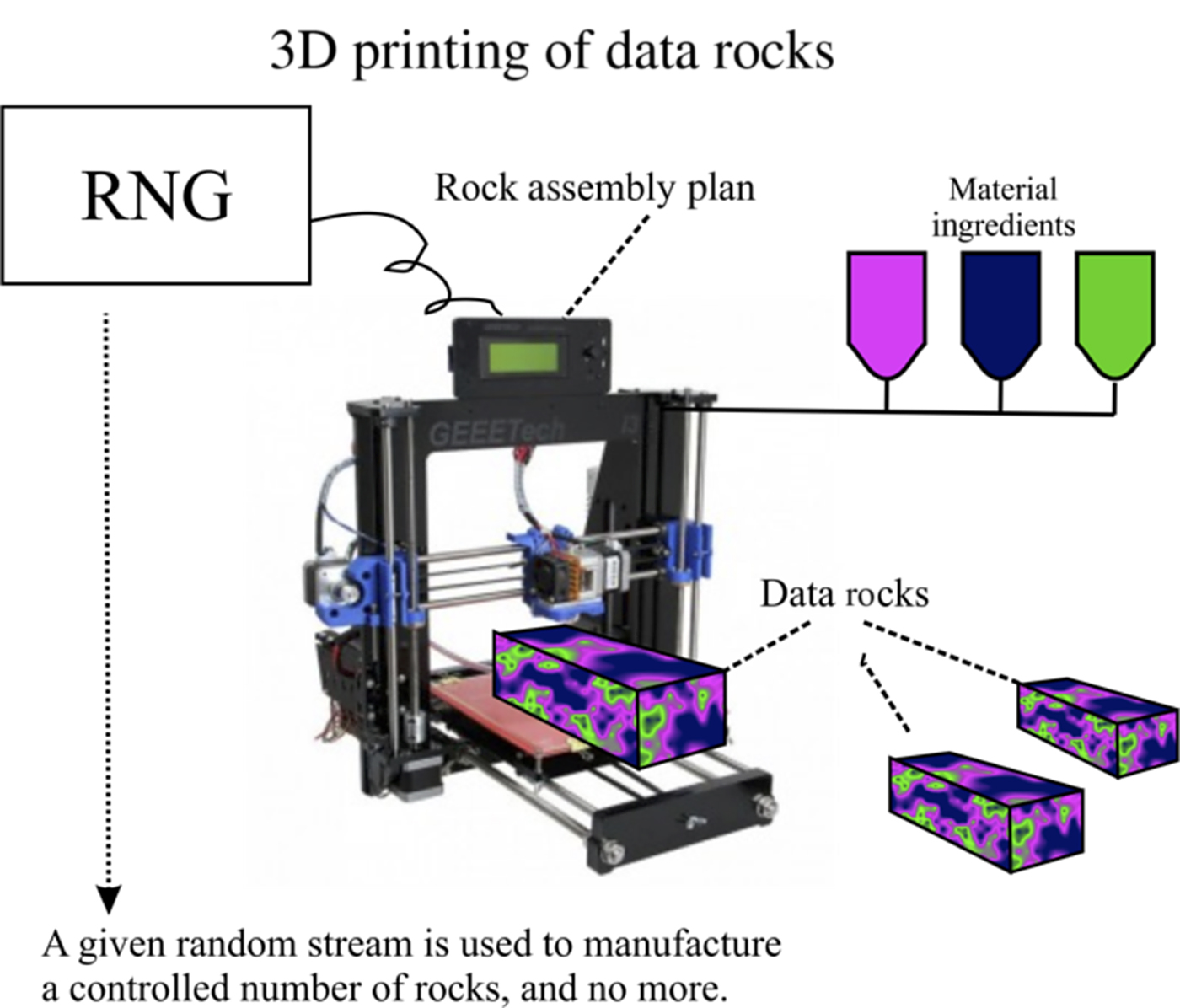
By far the most becoming rock manufacturing technique is 3D printing. As sketched in Fig. 2, the mathematically defined rock may be fed to the printer for execution of as many duplicates as desired. When done, the blueprint is destroyed to prevent additional printing.
Three-dimensional printing of a “rock”: a 3D printer is fed by stocks of all the ingredient materials, and is controlled by printing software fed by a random string of bits which is destroyed after printing. The feed randomness translates to the composition of the “rock.”
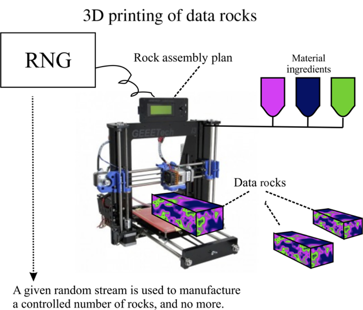
Alternatively, only the blocks geometry will be pre-defined and then forwarded as software to a 3D printer. The printer in real time would randomly choose the identity of which comprising material to use to fill any current block being printed. This choice will have to be temporarily recorded to manufacture the number of desired duplicates.
Three-dimensional printing technology[Reference Gibson, Rosen and Stucker13–Reference Babu, Love, Dehoff, Peter, Watkins and Pannala16] is already developed enough to insure the proper tolerance among the manufactured rocks. When a series is completed, the software driver for the blocks should be destroyed so no more rocks can be manufactured, and security can focus on the known number of rocks.
Today's technology of 3D printing is so advanced that a printing instruction package running on different machines will generate high-fidelity duplicates. This implies that a community of secure communicators does not have to rely on one manufacturing spot, and a subsequent physical distribution of the physical rocks, but rather rely on secure communication of the printing instruction package, and then, each party will generate its own rock. Of course the security of this strategy is limited by the security of communicating the printing instruction package, which can be achieved—poetically in a way—by using the secure randomness from a former rock. Hence, a community of secure communicators may end up communicating safely forever, by using one rock to generate a high-fidelity copy of the next.
An alternate method is entropic mixing where the entropy is fixed throughout the mixture, but it does not produce identical units as required. This method is still useful for cases where the rock is built to generate unshared randomness, as many randomness-rich ciphers now demand. The entropic mixing will require the mixed materials to be “mixable,” namely of manageable viscosity during the mix, and then solidify afterwards. Because of its non-repeatability, this method is ideal for unshared randomness.
Security analysis
The first security question is: can an attacker compromise the random rock without having a possession of the device? We consider an attacker that can query the rock as many times as desired. Submitting a specific pair of terminals, and getting an integer in reply. This attack can be carried out to the “brute force” limit, mapping all the possible answers. This attack may be counter-measured in several ways: (i) size—the random rock may be made so large, in terms of number of terminals that brute force attack will be infeasible; (ii) delayed response. The rock may be equipped with a delay option for repeat queries. (iii) The rock may be fitted with a counter that will allow normal queries, but will stop, or slow down considerably for repeated queries. These defenses apply also toward an insider who can toy with the rock, and query it at will.
The second question is: given a finite set of queries and their answers, is it feasible for an attacker to learn about the answers for additional queries. Since the construction of the rock is driven by high-quality randomness input, there is no established pattern which a smart attacker can discern, and so a finite set of queries will not become a source of compromise. If the attacker finds out somehow that a new query refers to terminals that are physically close to other pairs of terminals (physical terminal proximity), then there might be an inferential advantage. However, the rock is designed such that each terminal is planted in a zone of a different material than that of its neighbors, so the physical terminal proximity does not indicate read values similarity. Yet, it is helpful to keep the mapping matrix secret so that specifying terminals will not betray information regarding their physical proximity.
The next security question is: can an attacker who has a temporary possession of the rock compromise it? Such a possessor will be able to query the rock, and face the defenses identified above. Otherwise, without destroying the rock, the attacker will not be able to figure out its construction, and hence remain in the dark.
The next security question is: can an attacker who got a possession of everything relevant except the rock itself compromise the system? The answer is yes, with respect to the deterministic design features and with respect to the randomness that created the actual rock configuration. The rock security, then, depends on the diligence of the manufacturer to effectively hide the design and manufacturing guidance. The best way to do so is to destroy the randomness choices at least, and advisably also the deterministic design. This will prevent the manufacturer from manufacturing more rocks, but will prevent any theft, or compromise.
The next security question is: can an attacker, in possession of a rock, be able to duplicate it? It is difficult but possible. The attacker would have to “file away” the materials layer after layer, measure the dimensions of each block, identify the material in each block, then compile all that data to be fed into a 3D printer that will duplicate the rock. If the comprising materials are elemental metals, their identity will be readily revealed, but if they are seeded macromolecules, then the identification will be much more difficult. The smaller the rock, and the smaller the blocks that comprise it, the more difficult will it be to accurately measure the dimensions of the constituent blocks; and one will never know if the reconstruction was sufficiently accurate to generate the same output to queries. One may note that the attacker does not have to identify the exact material used in the rock, only to identify its exact conductivity, and then find a material with same conductivity. This may not always work because of electrical tension that builds up between the adjacent surfaces of the comprising materials which may impact the reading.
It would be hard to figure out the internal construction of the rock without taking it apart (destroying it). Any x-ray or similar method may not distinguish between the various comprising materials (which may be built from macromolecules) with different seeding, to engender different conductivity.
Dynamic randomness rock
The randomness rock as described above may be augmented into a dynamic version in the following way. After construction, one will select random spots on the surface, and drill holes of an arbitrary diameter, at an arbitrary depth, as long as those holes do not intersect. Into each of these holes, one will slide in a disruptive rod as shown in Fig. 3.
Randomness enhancing sliding rods: conducting rods positioned in the rock in different configurations affect the measured resistance, and enhance the variability of the readouts.

A disruptive rod is defined as a rod constructed of material with conductivity at the opposite spectrum from where the comprising materials are positioned—conductivity wise. That means that if the comprising materials are semi-conductors, or insulators, then the disruptive rods will be highly conductive metals. If the comprising materials will be highly-conductive metals, then the disruptive rods will be of poor conductivity.
The hole on the surface of the rock will be fitted with an exact sliding mechanism that would specify the depth to which the rod has been pushed into the drilled hole. It may span from no entry at all (the hole is fully empty) to full entry to occupy the entire hole. The state of the sliding rods in the rock will impact the reading of resistance between any two terminals on the rock.
To operate the dynamic rock, the communicating parties will agree on rod-settings in the open, and then will read the same measurements. The eavesdropper without the possession of the rock will be un-helped by the rod-setting information.
Given h holes to be drilled in the rock, where each rod can slide into its hole such that it can be stopped at s stops, then the rod setting will amount to a list of s position pairs (i,j), where i is the numeric identifier of the hole (1, 2, …h), and where j is the numeric identifier of the state of sliding of rod-i, where j = 1, 2, …s. Given such h pairs, the communicating parties will be able to agree on a particular setting in the set of sh settings, each with its own n(n−1)/2 readings. The total amount of reading associated with the dynamic random rock is:
 $${\bi s}^{\bi h}{\bi n}\lpar {{\bi n}-1} \rpar /2.$$
For a rock with n = 10,000 terminals, h = 10 rods with s = 20 sliding positing each, this amounts to more than 1020 readings, way above any possibility for post-imaging of the rock.
Applications
High-quality randomness is increasingly recognized as “cyber oil”, powering up the machinery of cyber space. The integrity of this modern form of life depends on preserving the integrity of the deployed randomness. The flip side here is that hackers and adversaries zero in on this very randomness to corrupt it and bent it to their purposes. Randomness becomes the battleground, and the very idea of housing it off-limit to the digital territory is a fundamental means for winning this cyber war. Usage then stretches to every protocol, every procedure, every cyber sequence in which randomness has a role, which is practically every action taken in the cyber world.
Here we will zero in on one fundamental application: Securing InterHub Critical Data Traffic. It is a common situation: several interconnected data centers are geographically spread, but functionally very tight. They exchange large amount of data between them, and use the public networks for the purpose. This exposed data, as it travels between the centers and as it resides in each center, is a prime target for adversarial action. Today this data is protected via the complex mathematics of modern cryptography. This protection is vulnerable to (i) advanced math attack, and to (ii) the imminent threat of quantum computers. Data at rest is also vulnerable to smart access procedures, which cannot be adequately protected against. To the extent that such hubs are critical, so is the need to cyber-protect them. This applies to major financial institutions, managing money flow around the globe; it applies to the power grid, and other infrastructure elements; it applies to military installations, etc.
In all these cases, the “Rock of Randomness” solution offers a simple guarantee: to successfully attack the protected system, it is necessary to secure physical access to the physical rock. While the data itself may be copied and replicated many times, and may be transported between the hubs back and forth, the key to read and interpret it is kept off the digital territory, is secured in the physical rock, and the only way to violate this data is by “touching” the rock. Unlike the maze of a computing center where a smart hacker may “get lost,” the physicality of the rock defines a clear perimeter of access. The rock may be physically shut down, and every request for access may be inspected with any desired scrutiny. In other words, the front line for cyber security has been shrunk to the enclosure of the rock, where all defensive measures should be concentrated. This is a game changer.
As it has been recently published, modern cyber security may shift from over-reliance on mathematical complexity to increased reliance on ever larger amounts of randomness.[Reference Samid17, Reference Samid18] On theoretical grounds, we know that sufficient randomness provides one with a mathematical guarantee of security,[Reference Samid18, Reference Samid19] and in general, the more randomness used, the greater the security of the data. With these facts in mind, it appears that the rock, functioning as a rich source of high-quality randomness, is a keystone for cyber security in the prospective future.
Future outlook
The Data Rock technology has the potential to pack very large quantities of randomness in reasonably sized physical rocks, to be shared among parties who practice secure communication. These quantities of quantum-grade packed randomness may be sufficient to enable all the communication between the secret sharing parties to achieve what Vernam proposed a century ago[Reference Vernam20]: perfect secrecy, without any fear of a super-smart attacker.
Quantum theory teaches us that at sub-atomic levels, measurements are not repeatable, and follow the probability curve indicated by Schrödinger's wave function. But this uncertainty vanishes fast at molecular, and in particular macromolecular, levels.
The only avenue of attack would be to take a hold of a physical rock. Guarding physical specimen is quite a different ballgame from insuring that running bits were not improperly exposed. It appears that materials science and engineering may hold the keys to the future of cryptography.