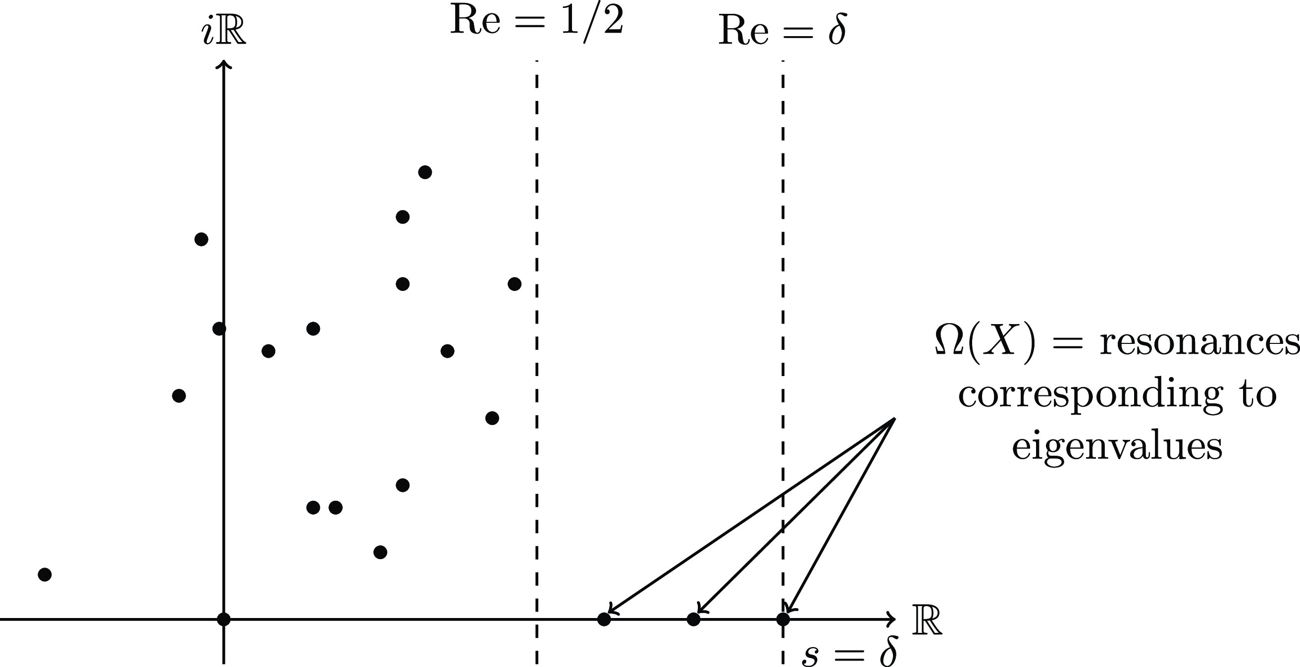






1. Introduction
1.1. Spectral gaps for congruence covers and main result
For each
 $q\in \mathbb{N}$
we denote by
 $X(q)$
the principal congruence cover of level
 $q$
of the modular surface
 $X = \mathrm{SL}_2(\mathbb{Z})\backslash {\mathbb{H}}^2$
and we let
 \begin{equation*} \lambda _0(q)=0\lt \lambda _1(q) \leqslant \lambda _2(q) \leqslant \ldots \end{equation*}
be the eigenvalues of the Laplace–Beltrami operator on
 $X(q)$
. In his seminal work [Reference Selberg38], Selberg famously proved that
 $\lambda _1(q) \geqslant \frac {3}{16}$
for all
 $q$
, and conjectured that
 $\lambda _1(q) \geqslant \frac {1}{4}$
. This remains one of the fundamental open problems of automorphic forms, although notable progress has been made in [Reference Iwaniec16, Reference Iwaniec and Gindikin17, Reference Kim, Ramakrishnan and Sarnak22, Reference Kim and Shahidi23, Reference Luo, Rudnick and Sarnak27], see also the expository articles of Sarnak [Reference Sarnak35, Reference Sarnak36].
In this paper, we consider congruence covers of quotients
 $X=\Gamma \backslash {\mathbb{H}}^2$
, where
 $\Gamma$
is an infinite-index subgroup of
 $ \mathrm{SL}_2({\mathbb{Z}})$
. Such groups, also called “thin” groups, do not come under the purview of the aforementioned papers. When
 $\Gamma$
is thin, the Hausdorff dimension of its limit set, denoted by
 $\delta$
, is strictly smaller than
 $1$
, and the quotient
 $X=\Gamma \backslash {\mathbb{H}}^2$
is an infinite-area hyperbolic surface. Moreover, the
 $L^2$
-spectrum of the Laplace–Beltrami operator
 $\Delta _X$
on
 $X$
is rather sparse, see Section 2.3 for more details. In the case where
 $\delta \gt \frac {1}{2}$
, only a finite number of eigenvalues exist, all are confined within the interval
 $\left [\delta (1-\delta ),\frac {1}{4} \right ]$
, and the smallest eigenvalue is given by
 $\lambda _0=\delta (1-\delta )$
. On the other hand, when
 $\delta \leqslant \frac {1}{2}$
, then no eigenvalues exist at all. Borthwick’s book [Reference Borthwick1] is an excellent reference for the spectral theory of infinite-area hyperbolic surfaces.
We focus on the case
 $\delta \gt \frac {1}{2}$
, and we define the multiset
 \begin{equation*} \Omega (X) \stackrel {\text{def}}{=} \left \{ s\in \left (\frac {1}{2},\delta \right ] :\, \text{$\lambda = s(1-s)$ is an $L^2$-eigenvalue of $\Delta _X$} \right \}, \end{equation*}
where each
 $s$
is repeated according to the multiplicity of
 $\lambda = s(1-s)$
as an eigenvalue of
 $\Delta _X$
. When
 $\Gamma$
is a subgroup of
 $\mathrm{SL}_2(\mathbb{Z})$
and
 $q\in \mathbb{N}$
, we define the principal congruence subgroup of
 $\Gamma$
of level
 $q$
as usual by
 \begin{equation} \Gamma (q) \stackrel {\text{def}}{=} \left \{ \text{$\gamma \in \Gamma $ : $\gamma \equiv I$ mod $q$} \right \}, \end{equation}
and we write
 $X(q) = \Gamma (q)\backslash {\mathbb{H}}^2$
for the associated covering.
Building on earlier work of Sarnak–Xue [Reference Sarnak and Xue37] for cocompact arithmeticFootnote
1
subgroups, Gamburd [Reference Gamburd12] proved the first analog of Selberg’s
 $\frac {3}{16}$
-theorem in the infinite-area setting:
Theorem 1.1 (Gamburd [Reference Gamburd12]). For every finitely generated subgroup
 $\Gamma \subset \mathrm{SL}_2(\mathbb{Z})$
with
 $\delta \gt \frac {5}{6}$
and for every large enough prime
 $p$
, we have
 \begin{equation} \Omega (X(p)) \cap \left ( \frac {5}{6}, \delta \right ] \stackrel {\text{m}}{=} \Omega (X) \cap \left ( \frac {5}{6}, \delta \right ], \end{equation}
where, for any two multisets
 $A$
and
 $B$
, we write
 $A \stackrel {\text{m}}{=} B$
if and only if the multiplicities of all elements are the same on both sides. In particular, if we denote by
 $\delta (1-\delta )=\lambda _0(q) \lt \lambda _1(q) \leqslant \cdots$
the eigenvalues of
 $X(q),$
then for all sufficiently large primes
 $p$
, we have
 \begin{equation*} \lambda _1(p)\geqslant \min \left \{ \frac {5}{36},\lambda _1(1) \right \}, \end{equation*}
provided both
 $\lambda _1(1)$
and
 $\lambda _1(p)$
exist.
Selberg’s
 $\frac {3}{16}$
-theorem and Gamburd’s
 $\frac {5}{36}$
-theorem have been extended as follows:
Theorem 1.2 (Bourgain–Gamburd–Sarnak [Reference Bourgain, Gamburd and Sarnak4]). For every finitely generated subgroup
 $\Gamma \subset \mathrm{SL}_2(\mathbb{Z})$
with
 $\delta \gt \frac {1}{2}$
, there exists
 $c = c(\Gamma )\gt 0$
such that for all square-free
 $q\in \mathbb{N}$
, we have
 \begin{equation} \Omega (X(q)) \cap \left [ \delta - c, \delta \right ] \stackrel {\text{m}}{=} \Omega (X) \cap \left [ \delta - c, \delta \right ]. \end{equation}
Analogous statements in terms of resonances when
 $\delta \leqslant \frac {1}{2}$
have been established by Oh–Winter [Reference Oh and Winter31] and Bourgain–Kontorovich–Magee [Reference Kontorovich, Bourgain and Magee19], see also [Reference Soares40]. The disadvantage of Theorem 1.2 (as with the results in [Reference Kontorovich, Bourgain and Magee19, Reference Oh and Winter31, Reference Soares40]) is that it does not provide an explicit gap. Apart from the intrinsic interest of this problem, explicit spectral gaps have many applications to concrete dynamical and arithmetic questions, see for instance [Reference Bourgain and Kontorovich5, Reference Ehrman10, Reference Hong and Kontorovich15, Reference Kontorovich24, Reference Kontorovich and Oh25].
Recently, Calderón–Magee [Reference Calderón and Magee7] improved Theorem 1.1 when
 $\Gamma$
is an arithmetic Schottky group. Schottky groups stand out, among other Fuchsian groups, by their simple geometric construction, which we recall in Section 2.6.
Theorem 1.3 (Calderón–Magee [Reference Calderón and Magee7]). For every Schottky group
 $\Gamma \subset \mathrm{SL}_2(\mathbb{Z})$
with
 $\delta \gt \frac {4}{5}$
and for every fixed
 $\sigma \gt \frac {1}{6}\delta + \frac {2}{3}$
there exists a constant
 $C = C(\Gamma ,\sigma )\gt 0$
such that for all
 $q\in \mathbb{N}$
whose prime divisors are all greater than
 $C$
, we have
 \begin{equation} \Omega (X(q)) \cap \left [ \sigma , \delta \right ] \stackrel {\text{m}}{=} \Omega (X) \cap \left [ \sigma , \delta \right ]. \end{equation}
In this paper, we pursue a similar goal as in [Reference Calderón and Magee7]. We wish to establish explicit spectral gaps that go beyond Gamburd’s
 $\frac {5}{36}$
-result. We are interested in “Hecke” congruence subgroups of Schottky groups
 $\Gamma \subset \mathrm{SL}_2(\mathbb{Z})$
:
 \begin{equation*} \Gamma _0(q) \stackrel {\text{def}}{=} \left \{ \gamma = \begin{pmatrix} a& \,\, b\\c& \,\, d\end{pmatrix}\in \Gamma : c\equiv 0\mod q\right \}. \end{equation*}
We write
 $X_0(q) = \Gamma _0(q) \backslash {\mathbb{H}}^2$
for the associated cover of
 $X$
. Note that since
 $ \Gamma (q)\subset \Gamma _0(q)$
, any eigenvalue for
 $X_0(q)$
is also one for
 $X(q)$
, and so the conclusion of Theorem 1.3 holds true for
 $X_0(q)$
as well. Our aim is to provide larger spectral gaps for
 $X_0(q)$
.
Let
 $P$
be the set of prime numbers. For any subset
 $P' \subseteq P$
, the natural density and the logarithmic density of
 $P'$
relative to
 $P$
are defined as
 \begin{equation*} d_{\mathrm{natural}}(P', P) \stackrel {\text{def}}{=} \lim _{x \to \infty } \frac {\sum _{\substack {p \leqslant x \\ p \in P'}} 1}{\sum _{\substack {p \leqslant x \\ p \in P}} 1} \end{equation*}
and
 \begin{equation*} d_{\mathrm{log}}(P', P) \stackrel {\text{def}}{=} \lim _{x \to \infty } \frac {\sum _{\substack {p \leqslant x \\ p \in P'}} \frac {1}{p}}{\sum _{\substack {p \leqslant x \\ p \in P}} \frac {1}{p}}, \end{equation*}
respectively, provided these limits exist.
For any
 $\frac {1}{2} \lt \sigma \lt \delta$
, we define
 $P_X(\sigma )$
as the set of primes
 $p$
satisfying
 \begin{equation} \Omega (X_0(p)) \cap \left [ \sigma , \delta \right ] \stackrel {\text{m}}{=} \Omega (X) \cap \left [ \sigma , \delta \right ]. \end{equation}
We can now state our main result as follows:
Theorem 1.4 (Main theorem). Let
 $\Gamma \subset \mathrm{SL}_2(\mathbb{Z})$
be a Schottky group and
 $\delta$
its Hausdorff dimension. The following statements hold true:
-
(i) Assume the Lindelöf Hypothesis for quadratic L-functions. Suppose that
 $\delta \gt \frac {3}{5}$
. Then, for any
$\sigma \gt \max \{ \frac {2}{3} \delta + \frac {1}{6}, \frac {1}{6}\delta + \frac {1}{2} \}$
, we have
$d_{\mathrm{log}}(P_X(\sigma ),P)=1$
.
-
(ii) Assume the generalized Riemann Hypothesis for quadratic L-functions. Suppose that
$\delta \gt \frac {3}{4}$
. Then, for any
$\sigma \gt \frac {5}{6}\delta$
, we have
$d_{\mathrm{natural}}(P_X(\sigma ),P)=1$
.






Although Theorem 1.4 is conditional and only guarantees spectral gaps for a density one subset of the primes, the explicit gaps obtained here are larger than those in Theorems 1.3 and 1.1, see Figure 1. Additionally, our result applies to a wider range of
 $\delta$
.
Spectral gaps as a function of
 $\delta$
.

By “quadratic”
 $L$
-functions, we mean the
 $L$
-functions
 $L(s, \chi _D)$
associated to the Kronecker symbol
 $\chi _D(\cdot ) = \left ( \frac {D}{\cdot }\right ).$
The generalized Riemann hypothesis (GRH) for the Dirichlet character
 $\chi$
is the assertion that if
 $s\in \mathbb{C}$
satisfies
 $L(s,\chi )=0$
and if
 $s$
is a not a negative integer, then
 $s$
has real part
 $\frac {1}{2}.$
The Lindelöf hypothesis for the Dirichlet L-function
 $L(s,\chi )$
with a character
 $\chi$
modulo
 $q$
states that, for all
 $t\in \mathbb{R}$
and
 $\epsilon \gt 0$
,
 \begin{equation} \left \vert L\left (\frac {1}{2}+it, \chi \right ) \right \vert \ll _\epsilon q^\epsilon (1+\vert t\vert )^\epsilon . \end{equation}
It is well known that the Lindelöf hypothesis follows from the GRH, see [Reference Iwaniec and Kowalski18, Corollary 5.20].
Coincidentally, Theorem 1.4 is similar in spirit to an early result of Iwaniec [Reference Iwaniec16], even though it was proven by different methods and deals only with the case
 $\Gamma =\mathrm{SL}_2({\mathbb{Z}})$
. This result says that for almost all primes
 $p$
, the first eigenvalue of the Laplacian for the level
 $p$
Hecke congruence group of
 $\mathrm{SL}_2({\mathbb{Z}})$
twisted by a certain multiplier
 $\chi _p$
is larger or equal to
 $\frac {44}{225}$
. This has later been superseded by [Reference Iwaniec and Gindikin17, Reference Kim and Shahidi23, Reference Luo, Rudnick and Sarnak27], with the current best spectral gaps for congruence subgroups of
 $\mathrm{SL}_2({\mathbb{Z}})$
being established by Kim–Sarnak [Reference Kim, Ramakrishnan and Sarnak22].
We will actually prove a slightly stronger result than Theorem 1.4. We call an eigenvalue for
 $X_0(q)$
“new” if it occurs with greater multiplicity than in
 $X$
. We denote, by
 $N_\Gamma ^{\mathrm{new}}(q, \sigma )$
, the number of new eigenvalues of the form
 $\lambda = s(1-s)$
with
 $s\in [\sigma , \delta ]$
, where eigenvalues are counted according to multiplicity. Then, we have
Theorem 1.5 (Main theorem, elaborated). Under the hypotheses of Theorem 1.4
, the following conditional estimates hold for any
 $x \gt 1$
,
 $\epsilon \gt 0$
, and
 $\sigma \in [\frac {1}{2}, \delta ]$
:
-
(i) Assume the Lindelöf Hypothesis for quadratic
$L$
-functions. If
$\delta \gt \frac {1}{2}$
, then
where
\begin{equation*} \sum _{\substack {2 \leqslant q \leqslant x \\ \text{$q$ square-free}}} N_\Gamma ^{\mathrm{new}}(q, \sigma ) \leqslant C(\epsilon , \Gamma ) \cdot \max \left \{ x, x^{1 - \frac {2}{A} \left ( \sigma - \frac {\delta + A}{2} \right ) + \epsilon } \right \}, \end{equation*}
$A = \max \left \{ \frac {1 + \delta }{3}, 1 - \frac {2}{3} \delta \right \}.$
-
(ii) Assume the Generalized Riemann Hypothesis for quadratic
$L$
-functions. If
$\delta \gt \frac {3}{4}$
, then
where
\begin{equation*} \sum _{\substack {2 \leqslant p \leqslant x \\ \text{$p$ prime}}} N_\Gamma ^{\mathrm{new}}(p, \sigma ) \leqslant C(\epsilon , \Gamma ) \cdot x^{1 - \frac {2}{A} \left ( \sigma - \frac {\delta + A}{2} \right ) + \epsilon }, \end{equation*}
$A = \frac {2\delta }{3}.$


The constant
 $C(\epsilon , \Gamma ) \gt 0$
depends only on
 $\epsilon$
and the Schottky data of
 $\Gamma$
.
Proof that Theorem 1.5 implies Theorem 1.4
. Let
 $B_X(\sigma ) = P\setminus P_X(\sigma )$
be the set of “bad” primes, that is, the primes
 $p$
for which
 $N_\Gamma ^{\mathrm{new}}(p,\sigma ) \geqslant 1$
.
We start with proving the second part of Theorem 1.4. Our goal is to establish that
 $B_X(\sigma )$
has zero natural density with respect to the primes, provided
 $\sigma \gt \frac {5}{6}\delta .$
By the second part of Theorem 1.5, we have
 \begin{equation*} \#B_X(\sigma ) \cap \{ p\leqslant x \} = O_{\epsilon ,\Gamma }\left (x^{1 - \frac {3}{\delta } ( \sigma - \frac {5}{6}\delta ) + \epsilon }\right ). \end{equation*}
Hence, for each fixed
 $\sigma \gt \frac {5}{6}\delta$
, it follows that the left-hand side is less than
 $O_\eta (x^{1-\eta })$
for any
 $\eta \gt 0$
sufficiently small in terms of
 $\sigma .$
On the other hand, by the prime number theorem, there are roughly
 $\frac {x}{\log (x)}$
primes not exceeding
 $x$
, and hence, we conclude that
 $d_{\mathrm{natural}}(B_X(\sigma ),P)=0$
.
Now, we deduce the first part of Theorem 1.4. Here, our goal is to establish that
 $B_X(\sigma )$
has zero logarithmic density with respect to the primes, provided
 $\sigma \gt \max \{ \frac {2}{3} \delta + \frac {1}{6}, \frac {1}{6}\delta + \frac {1}{2} \}$
. The proof relies on the following observation: for any
 $q\in \mathbb{N}$
, we have
 \begin{equation*} N_\Gamma ^{\mathrm{new}}(q,\sigma ) \geqslant \sum _{\substack {p\mid q \\ p\in P}} N_\Gamma ^{\mathrm{new}}(p,\sigma ), \end{equation*}
where the sum is over the prime divisors of
 $q$
. This follows for instance from (63). Summing this inequality over all square-free integers
 $q\in [2,x]$
yields
 \begin{align*} \sum _{\substack {q\leqslant x}} N_\Gamma ^{\mathrm{new}}(q,\sigma ) &\geqslant \sum _{\substack {q\leqslant x}} \sum _{\substack {p\mid q \\ p\in P}} N_\Gamma ^{\mathrm{new}}(p,\sigma ) \\ &\geqslant \sum _{\substack {p\leqslant x \\ p\in P}} N_\Gamma ^{\mathrm{new}}(p,\sigma ) \left ( \sum _{\substack {q \leqslant x \\ p\mid q}} 1 \right )\\ &\gg x \sum _{\substack {p\leqslant x \\ p\in P}} \frac {N_\Gamma ^{\mathrm{new}}(p,\sigma )}{p}. \end{align*}
Rearranging gives
 \begin{equation} \sum _{\substack {p\leqslant x \\ p\in P}} \frac {N_\Gamma ^{\mathrm{new}}(p,\sigma )}{p} \ll \frac {1}{x} \sum _{\substack {q\leqslant x}} N_\Gamma ^{\mathrm{new}}(q,\sigma ). \end{equation}
Now, let
 $A = \max \left \{ \frac {1+\delta }{3}, 1-\frac {2}{3}\delta \right \}$
be as in Part (i) of Theorem 1.5, and note that
 \begin{equation*} \frac {\delta + A}{2} = \max \left \{ \frac {2}{3} \delta + \frac {1}{6}, \frac {1}{6}\delta + \frac {1}{2} \right \}. \end{equation*}
We can now apply the Part (i) of Theorem 1.5 to deduce (assuming the Lindelöf Hypothesis for quadratic L-functions) that for each fixed
 $\sigma \gt \max \{ \frac {2}{3} \delta + \frac {1}{6}, \frac {1}{6}\delta + \frac {1}{2} \}$
,
 \begin{equation} \sum _{\substack {q\leqslant x}} N_\Gamma ^{\mathrm{new}}(q,\sigma ) \ll _\sigma x. \end{equation}
Combining (7) and (8) and recalling the definition of
 $B_X(\sigma )$
, we find
 \begin{equation*} \sum _{\substack {p\leqslant x \\ p\in B_X(\sigma )}} \frac {1}{p} \ll \frac {1}{x}\sum _{\substack {q \leqslant x}} N_\Gamma ^{\mathrm{new}}\left ( q,\sigma \right ) \ll _\sigma 1. \end{equation*}
Using the well-known estimate
 \begin{equation*} \sum _{\substack {p\leqslant x \\ p\in P}} \frac {1}{p} \gg \log \log x, \end{equation*}
it now follows that
 $d_{\mathrm{log}}(B_X(\sigma ),P)=0$
.
1.2. Thick arithmetic Schottky groups
At this point, the reader may wonder whether Schottky subgroups of
 $\mathrm{SL}_2(\mathbb{Z})$
with
 $\delta \gt \frac {3}{4}$
actually exist. In fact, we can construct a sequence of Schottky groups
 $(\Gamma _m)_{m\in \mathbb{N}}$
satisfying
 $\delta _{m} = \delta (\Gamma _m)\to 1$
as
 $m\to \infty$
by taking
 \begin{equation*} \Gamma _m \stackrel {\text{def}}{=} \langle g_1^\pm , \ldots , g_m^\pm \rangle \subset \mathrm{SL}_2(\mathbb{Z}), \quad g_k = \begin{pmatrix} 3k&9k^2-1\\1&3k\end{pmatrix}. \end{equation*}
It is not hard to verify that
 $g_k$
maps the exterior of the disk
 $B_{k} = \{ z\in \mathbb{C} : \vert z+3k\vert \lt 1 \}$
to the interior of
 $B_{-k} = \{z\in \mathbb{C} : \vert z-3k\vert \lt 1 \}$
. Clearly, the disks
 $B_{1}, \ldots , B_{m}, B_{-1}, \ldots , B_{-m}$
are centered on the real line and have mutually disjoint closures, so
 $\Gamma _m$
is a Schottky group in the sense of the definition in Section 2.6. Moreover,
 $\mathcal{F}_m = {\mathbb{H}}^2\smallsetminus (B_{1}\cup \ldots \cup B_{m} \cup B_{-1}\cup \ldots \cup B_{-m})$
provides a fundamental domain for
 $ \Gamma _m \backslash {\mathbb{H}}^2$
. To see that
 $\delta _m \to 1$
, we borrow an argument from Gamburd at the end of his paper [Reference Gamburd12]. The base eigenvalue of
 $\Gamma _m \backslash {\mathbb{H}}^2$
equals
 $\lambda _0(\Gamma _m) = \delta _{m} (1-\delta _{m})$
. On the other hand, the variational characterization of the base eigenvalue says that
 \begin{equation*} \lambda _0(\Gamma _m) = \inf _{\substack { u\in L^2(\mathcal{F}_m) \\ \nabla u \in L^2(\mathcal{F}_m) }} \frac {\int _{\mathcal{F}_m} \vert \nabla u \vert ^2 d\mu }{\int _{\mathcal{F}_m} u^2 d\mu }, \quad d\mu = \frac {dx dy}{y^2}. \end{equation*}
Similarly to [Reference Gamburd12], our fundamental domain
 $\mathcal{F}_m$
is an exterior of mutually disjoint Euclidean disks of radius one and centered on the real line. Therefore, we can use suitable test-functions
 $u$
on
 $\mathcal{F}_m$
similar to those in [Reference Gamburd12] to show that
 $\lambda _0(\Gamma _m) \to 0$
. From this, we conclude that
 $\delta _m\to 1$
.
1.3. Outline of proof
We now sketch the proof of Theorem 1.5. For the sake of exposition, we will concentrate on the second part of the theorem, since this is enough to convey the key concepts of the argument. The methods in the papers quoted at the beginning of the introduction [Reference Iwaniec16, Reference Iwaniec and Gindikin17, Reference Kim, Ramakrishnan and Sarnak22, Reference Kim and Shahidi23, Reference Luo, Rudnick and Sarnak27, Reference Selberg38] do not easily generalize to thin groups and rather new tools are required. Our proof builds on the same techniques used in [Reference Calderón and Magee7, Reference Naud and Magee30, Reference Soares39].
Let
 $\lambda _q \stackrel {\text{def}}{=} \mathrm{Ind}_{\Gamma _0(q)}^\Gamma (\textbf {1}_{\Gamma _0(q)})$
be the representation of
 $\Gamma$
induced from the trivial representation on
 $\Gamma _0(q)$
, and let
 $\lambda _q^0 \stackrel {\text{def}}{=} \lambda _q \ominus \textbf {1}_{\Gamma }$
denote its non-trivial part. By the Venkov–Zograf formula (23), new eigenvalues
 $\lambda = s(1-s)$
for
 $X_0(q)$
correspond to zeros
 $s$
of the twisted Selberg zeta function
 $Z_{\Gamma }(s,\lambda _q^0)$
in the interval
 $\left [ \frac {1}{2},\delta \right ]$
. Our aim is to estimate the number of such zeros in
 $\left [ \sigma ,\delta \right ]$
for any
 $\frac {1}{2}\lt \sigma \lt \delta$
.
Let us briefly recall the thermodynamic formalism for the twisted Selberg zeta function. For any finite-dimensional unitary representation
 $\rho \colon \Gamma \to \mathrm{U}(V)$
, there is an associated (
 $\rho$
-twisted) transfer operator
 $\mathcal{L}_{s,\rho }$
whose Fredholm determinant equals the Selberg zeta function:
 \begin{equation} Z_{\Gamma }(s,\rho ) = \det (1-\mathcal{L}_{s,\rho }). \end{equation}
This operator is defined explicitly in terms of the Schottky data of
 $\Gamma$
(see Section 2.8). In this paper, we work with the refined transfer operators
 $\mathcal{L}_{\tau ,s,\rho }$
(see Section 2.9), introduced by Dyatlov–Zworski [Reference Dyatlov and Zworski9]. These operators are accelerated versions of
 $\mathcal{L}_{s,\rho }$
, with the acceleration controlled by a small parameter
 $\tau \gt 0$
. A key fact from [Reference Dyatlov and Zworski9] is that any 1-eigenfunction of
 $\mathcal{L}_{s,\rho }$
is also a 1-eigenfunction of
 $\mathcal{L}_{\tau ,s,\rho }$
. In this paper, we use a stronger result (Lemma 2.2): the refined zeta function
 \begin{equation} \zeta _{\tau }(s,\rho ) \stackrel {\text{def}}{=} \det \left ( 1 - \mathcal{L}_{\tau ,s,\rho }^{2} \right ) \end{equation}
is equal to the Selberg zeta function times an entire function. Therefore, every zero of the Selberg zeta function is also a zero of
 $\zeta _{\tau }(s,\rho )$
, with at least the same multiplicity.
While this approach may initially appear overly complicated, it ultimately yields explicit estimates for the number of zeros of the Selberg zeta function. The key point is choosing the parameter
 $\tau$
that yields the optimal upper bounds. Using Jensen’s formula from complex analysis, the number of zeros of
 $\zeta _{\tau }(s,\rho )$
inside
 $[\sigma ,\delta ]$
can be bounded in terms of the Hilbert–Schmidt norm
 $\Vert \mathcal{L}_{\tau ,s,\rho }\Vert _{\mathrm{HS}}$
for
 $s\approx \sigma .$
The representations
 $\rho$
appearing in this paper are the representations
 $\lambda _q^0$
described above. Estimating the HS-norm
 $\Vert \mathcal{L}_{\tau ,s,\lambda _q^0}\Vert _{\mathrm{HS}}$
for individual
 $q$
seems quite difficult. However, assuming the GRH for quadratic L-functions, we can non-trivially estimate the sum
 \begin{equation} \sum _{\substack {x/2 \lt p \leqslant x \\ \text{$p$ prime}}} \Vert \mathcal{L}_{\tau ,s,\lambda _p^0}\Vert _{\mathrm{HS}}^2. \end{equation}
This constitutes the main novelty in this paper. We note that the first part of Theorem 1.5 requires more involved sums over square-free integers, and in this case, we prove similar non-trivial estimates conditional on the weaker Lindelöf Hypothesis.
Thanks to the explicit formula for the Hilbert–Schmidt norm in Lemma 2.8, estimating (11) reduces to estimating sums of the form
 \begin{equation} \sum _{\substack { x/2 \lt p\leqslant x \\ \text{$p$ prime} }} \mathrm{tr}( \lambda _p^0(\gamma ) ) \end{equation}
for fixed
 $\gamma \in \Gamma .$
We prove that unless
 $\gamma \in \Gamma$
equals
 $\pm I$
modulo
 $p$
, then
 \begin{equation*} \mathrm{tr}( \lambda _p^0(\gamma ) ) = \left ( \frac {\mathcal{D}(\gamma )}{p}\right ), \quad \mathcal{D}(\gamma )\stackrel {\text{def}}{=} \textrm {tr}(\gamma )^2-4, \end{equation*}
where
 $\left ( \frac {\cdot }{p}\right )$
is the Kronecker symbol modulo
 $p$
. Hence, we are faced with understanding the asymptotic behavior of the character sum
 \begin{equation} \sum _{\substack { x/2 \lt p\leqslant x \\ \text{$p$ prime} }} \chi _{D}(n), \quad \chi _{D}(n) = \left ( \frac {D}{n} \right ), \end{equation}
as
 $x\to \infty$
, for fixed
 $D$
. It is here where GRH comes into play. If
 $D$
is a positive integer with
 $D = 0,1,2 \mod 4$
, then
 $ \chi _{D}(n)$
is a Dirichlet character of conductor at most
 $4D$
. Conditional on GRH, for all such
 $D$
, the modulus of (13) is bounded by
 $O_\epsilon (x^{1/2+\epsilon } D^\epsilon ).$
Inserting this into (11) and choosing
 $\tau \gt 0$
optimally in terms of
 $x$
, we find
 \begin{equation} \sum _{\substack { x/2 \lt p\leqslant x \\ \text{$p$ prime} }} \Vert \mathcal{L}_{\tau ,s,\lambda _p^0}\Vert _{\mathrm{HS}}^2 \ll _\epsilon x^{1-\frac {3}{\delta }( \sigma -\frac {5}{6}\delta ) + \epsilon }. \end{equation}
The precise statement is given in Proposition 4.3. This implies that for a “typical” prime
 $p$
, one has
 \begin{equation*} \Vert \mathcal{L}_{\tau ,s,\lambda _p^0}\Vert _{\mathrm{HS}}^2 = O_\epsilon \left (p^{- \frac {3}{\delta }(\sigma - \frac {5}{6}\delta )+\epsilon }\right ). \end{equation*}
The second statement of Theorem 1.5 now follows easily.
We note that the actual proof deviates considerably from the description given here. For instance, to establish (14), several distortion estimates for Schottky groups are required. These estimates are mostly well-known from the papers [Reference Naud29, Reference Naud and Magee30] and we record them in Section 2.10.
We point out that uniformity in the estimates of the character sums (13) with respect to the parameter
 $D$
is vital for us. To the best of the author’s knowledge, all existing unconditional bounds for these character sums exhibit a strong dependence on the conductor. In our specific application, we must be able to bound the sum in (13) even when
 $D$
becomes quite large, approximately on the order of
 $D \approx x^B$
for some absolute constant
 $B \gt 0$
. Relying solely on unconditional bounds would lead to rather weak (and, in fact, useless) estimates in (14).
Finally, it would be interesting to explore whether the techniques employed in this work yield novel results for similar families of lattices in
 $\mathrm{SL}_2(\mathbb{R}).$
1.4. Organization of the paper
In Section 2, we gather the basic definitions and tools needed for our main proof of Theorem 1.4. This includes a review of Schottky groups, the introduction of refined transfer operators, and the description of the function spaces on which these operators act. Section 3 establishes the connection between the number of zeros of the Selberg zeta functions and the refined transfer operators. Finally, the proof of Theorem 1.4 is given in Section 4, which is organized into several subsections.
1.5. Notation
We write
 $f(x) \ll g(x)$
or
 $f(x) = O(g(x))$
interchangeably to mean that there exists a constant
 $C \gt 0$
such that
 $|f(x)| \leqslant C |g(x)|$
. We write
 $f(x) \ll _y g(x)$
or
 $f(x) = O_y(g(x))$
to indicate that the implied constant
 $C$
depends on the parameter
 $y$
. We may also write
 $C = C(y)$
to emphasize this dependence. The notation
 $f(x) = o(g(x))$
will be used to indicate that
 $g(x)/f(x) \to 0$
as
 $x \to \infty$
. Whenever we write
 $s = \sigma + it \in \mathbb{C}$
, we mean that
 $\sigma$
and
 $t$
are the real and imaginary parts of the complex number
 $s$
, respectively. Given a finite set
 $S$
, we denote its cardinality by
 $|S|$
or
 $\# S$
. Finally, we use the shorthand
 $p \sim x$
to mean
 $x/2 \lt p \leqslant x$
.
2. Preliminaries
2.1. Hyperbolic geometry
Let us recall some basic facts about hyperbolic surfaces, referring the reader to Borthwick’s book [Reference Borthwick1] for a comprehensive discussion. One of the standard models for the hyperbolic plane is the Poincaré half-plane
 \begin{equation*} {\mathbb{H}}^2=\{ x+iy\in {\mathbb{C}}\ :\ y\gt 0\} \end{equation*}
endowed with its standard metric of constant curvature
 $-1$
,
 \begin{equation*} ds^2=\frac {dx^2+dy^2}{y^2}. \end{equation*}
The group of orientation-preserving isometries of
 $({\mathbb{H}}^2, ds)$
is isomorphic to
 $\mathrm{PSL}_2({\mathbb{R}})$
. It acts on the extended complex plane
 $\overline {{\mathbb{C}}} = {\mathbb{C}} \cup \{ \infty \}$
(and hence also on
 ${\mathbb{H}}^2$
) by Möbius transformations
 \begin{equation*} \gamma =\begin{pmatrix} a&b\\c&d\end{pmatrix}\in \mathrm{PSL}_2({\mathbb{R}}),\quad z\in \overline {{\mathbb{C}}} \Longrightarrow \gamma (z) = \frac {az+b}{cz+d}. \end{equation*}
A non-identity element
 $\gamma \in \mathrm{PSL}_2({\mathbb{R}})$
is either
-
• hyperbolic if
$\vert \mathrm{tr}(\gamma )\vert \gt 2$
, which implies that
$\gamma$
has two distinct fixed points on the boundary
$\partial {\mathbb{H}}^2$
, -
• parabolic if
$\vert \mathrm{tr}(\gamma )\vert =2$
, which implies that
$\gamma$
has precisely one fixed point on
$\partial {\mathbb{H}}^2$
, or -
• elliptic if
$\vert \mathrm{tr}(\gamma )\vert \lt 2$
, which implies that
$\gamma$
has precisely one fixed point in the hyperbolic plane
${\mathbb{H}}^2$
.


2.2. Hyperbolic surfaces and Fuchsian groups
Every hyperbolic surface
 $X$
is isometric to a quotient
 $\Gamma \backslash {\mathbb{H}}^2$
, where
 $\Gamma$
is a Fuchsian group, that is, a discrete subgroup
 $\Gamma \subset \mathrm{PSL}_2({\mathbb{R}})$
. A Fuchsian group
 $\Gamma$
is called
-
• torsion-free if it contains no elliptic elements,
-
• non-cofinite if the quotient
$\Gamma \backslash {\mathbb{H}}^2$
has infinite-area, -
• non-elementary if it is generated by more than one element, and
-
• geometrically finite if it is finitely generated, which is equivalent with
$\Gamma \backslash {\mathbb{H}}^2$
being geometrically and topologically finite.


The Fuchsian groups
 $\Gamma$
considered in this paper satisfy all the above conditions. The limit set
 $\Lambda$
of
 $X$
is a fractal subset of the boundary
 $\partial {\mathbb{H}}^2 \cong \mathbb{R}\cup \{ \infty \}$
, consisting of accumulation points of all orbits of the action of
 $\Gamma$
on
 ${\mathbb{H}}^2$
. It has a Cantor-like structure and its Hausdorff dimension, denoted by
 $\delta$
, lies strictly between
 $0$
and
 $1$
.
Furthermore,
 $\Gamma$
is called convex cocompact if it is finitely generated and if it contains neither parabolic nor elliptic elements. This is equivalent with the convex core of
 $X = \Gamma \backslash {\mathbb{H}}^2$
being compact. By a result of Button [Reference Button6], every infinite-area, convex cocompact hyperbolic surface
 $X$
can be realized as the quotient of
 ${\mathbb{H}}^2$
by a so-called Schottky group
 $\Gamma$
, which we will define in Section 2.6 below, see also [Reference Borthwick1, Theorem 15.3].
Since we work exclusively with torsion-free Fuchsian groups, the distinction between
 $\mathrm{PSL}_2({\mathbb{R}})$
and
 $\mathrm{SL}_2({\mathbb{R}})$
is immaterial. Hence, we will use
 $\mathrm{SL}_2({\mathbb{R}})$
throughout this paper.
2.3. Spectral theory of infinite-area hyperbolic surfaces
Let us review some aspects of the spectral theory of infinite-area hyperbolic surfaces. Again, we refer the reader to [Reference Borthwick1] for an in-depth account of the material given here. The
 $ L^{2}$
-spectrum of the Laplace–Beltrami operator
 $\Delta _X$
on an infinite-area hyperbolic surface
 $X$
was described by Lax–Phillips [Reference Lax and Phillips26] and Patterson [Reference Patterson32] as follows:
-
• The absolutely continuous spectrum is equal to
$ [1/4, \infty )$
. -
• The pure point spectrum is finite and contained in the interval
$(0,1/4)$
. In particular, there are no eigenvalues embedded in the continuous spectrum. -
• If
$\delta \leqslant 1/2$
, then the pure point spectrum is empty. If
$\delta \gt 1/2$
, then
$\lambda _0(X) = \delta (1-\delta )$
is the smallest eigenvalue.


In light of these facts, the resolvent operator
 \begin{equation*} R_X(s) \stackrel {\text{def}}{=} \big ( \Delta _X - s(1-s)\big )^{-1}\colon L^2(X) \to L^2(X) \end{equation*}
is defined for all
 $s\in {\mathbb{C}}$
with
 $ \mathrm{Re}(s)\gt 1/2$
and
 $s(1-s)$
not being an
 $L^2$
-eigenvalue of
 $\Delta _X$
. From Guillopé–Zworski [Reference Guillopé and Zworski14], we know that the resolvent extends to a meromorphic family
 \begin{equation} R_X(s) \colon C_{c}^{\infty }(X) \to C^{\infty }(X) \end{equation}
on
 $\mathbb{C}$
with poles of finite rank. The poles of
 $R_X(s)$
are called the resonances of
 $ X$
and the multiplicity of a resonance
 $\zeta$
is the rank of the residue operator of
 $R_X(s)$
at
 $s=\zeta$
. We denote by
 $\mathcal{R}(X)$
the set multiset of resonances of
 $X$
repeated according to multiplicities. Resonances are contained in the half-plane
 $\mathrm{Re}(s)\leqslant \delta$
. There is a simple resonance at
 $s=\delta$
; there are no other resonances on the vertical line
 $\mathrm{Re}(s)=\delta$
. Any resonance
 $s$
on the half-plane
 $\mathrm{Re}(s)\gt \frac {1}{2}$
corresponds to an eigenvalue
 $\lambda = s(1-s)$
of
 $\Delta _X$
, see Figure 2. In other words, the set
 $\Omega (X)$
defined in the introduction can be re-expressed as
 \begin{equation*} \Omega (X) \stackrel {\text{m}}{=} \mathcal{R}(X) \cap \left \{ \mathrm{Re}(s) \gt \frac {1}{2} \right \}. \end{equation*}
In particular,
 $\Omega (X)$
is empty for
 $\delta \leqslant \frac {1}{2}$
.
The
 $s$
-plane: distribution of resonances for infinite-area
 $ \Gamma \backslash {\mathbb{H}}^2$
in the case
 $ \delta \gt \frac {1}{2}$
.

2.4. Twisted Selberg zeta function
Let
 $\Gamma \subset \mathrm{PSL}_2({\mathbb{R}})$
be a finitely generated Fuchsian group. The set of prime periodic geodesics on
 $X=\Gamma \backslash {\mathbb{H}}^2$
is bijective to the set
 $[\Gamma ]_{\mathsf{prim}}$
of
 $\Gamma$
-conjugacy classes of primitive hyperbolic elements in
 $\Gamma$
. We denote by
 $\ell (\gamma )$
the length of the geodesic corresponding to the conjugacy class
 $[\gamma ] \in [\Gamma ]_{\mathsf{prim}}$
.
The Selberg zeta function is defined for
 $\mathrm{Re}(s) \gt \delta$
by the infinite product
 \begin{equation} Z_{\Gamma }(s)\stackrel {\text{def}}{=}\prod _{k=0}^\infty \prod _{[\gamma ] \in [\Gamma ]_{\mathsf{prim}}}\left ( 1 - e^{-(s+k)\ell (\gamma )}\right ), \end{equation}
and it has a meromorphic continuation to
 $s\in \mathbb{C}.$
There is a beautiful correspondence between resonances of
 $X$
and the zeros of
 $Z_\Gamma (s)$
established in [Reference Borthwick, Judge and Perry2, Reference Patterson and Perry33]. Concretely, the zero set of
 $Z_\Gamma (s)$
consists of the following:
-
• “Topological” zeros at the non-positive integers. The topological zero at
$s=-k$
with
$k\in \mathbb{N}_0$
has multiplicity
$-(2k+1)\chi (X).$
-
• The set
$\mathcal{R}(X)$
of resonances of
$X$
.


Moreover, if
 $\Gamma$
has no parabolic elements, which is the case of interest to us, then
 $Z_\Gamma (s)$
has no poles. We note that the resonances and the topological zeros could potentially overlap at
 $-\mathbb{N}_0$
. However, outside this set, the multiplicity of a zero
 $s$
of
 $Z_\Gamma (s)$
matches its multiplicity as a resonance of
 $X$
. In particular, the first zero of
 $Z_\Gamma (s)$
(furthest to the right) is the simple resonance at
 $s=\delta$
. Therefore, any problem about resonances and eigenvalues can be rephrased as a question about the distribution of the zeros of the Selberg zeta function.
Let
 $(\rho ,V)$
be a finite-dimensional unitary representation of
 $\Gamma$
. Consider the twisted Selberg zeta function
 \begin{equation} Z_{\Gamma }(s,\rho )\stackrel {\text{def}}{=}\prod _{k=0}^\infty \prod _{[\gamma ] \in [\Gamma ]_{\mathsf{prim}}} \det \nolimits _V\left ( I_V - \rho (\gamma )e^{-(s+k)\ell (\gamma )}\right ). \end{equation}
Clearly, if
 $\rho = \textbf {1}_{\mathbb{C}}$
is the trivial, one-dimensional representation of
 $\Gamma$
, then (17) reduces to classical Selberg zeta function (16). Furthermore, the product definition (17) implies that
 \begin{equation} Z_\Gamma (s,\rho _1 \oplus \rho _2) = Z_\Gamma (s,\rho _1)Z_\Gamma (s,\rho _2), \end{equation}
where
 $\rho _1 \oplus \rho _2$
denotes the orthogonal direct sum of
 $\rho _1$
and
 $\rho _2$
.
2.5. Venkov–Zograf induction formula
One of the main properties of twisted Selberg zeta functions is the Venkov–Zograf induction formula [Reference Venkov41, Reference Venkov and Zograf42]. It states that for any finite-index subgroup
 $\Gamma '\subset \Gamma$
the following relationship holds true:
 \begin{equation} Z_{\Gamma '}(s) = Z_\Gamma (s,\lambda _{\Gamma /\Gamma '}), \end{equation}
where
 \begin{equation} \lambda _{\Gamma /\Gamma '} \stackrel {\text{def}}{=} \mathrm{Ind}_{\Gamma '}^{\Gamma }(\textbf {1}_{\Gamma '}) \end{equation}
is the induced representation of the trivial one-dimensional representation
 $\textbf {1}_{\Gamma '}$
of
 $\Gamma '$
to the larger group
 $\Gamma .$
We also refer to the more recent paper [Reference Fedosova and Pohl11] for a proof of this formula based on the Frobenius character formula.
Let
 $g_1, \ldots , g_n$
be a full set of representatives in
 $\Gamma$
of the left cosets in
 $\Gamma /\Gamma '$
, where
 $n=[\Gamma :\Gamma ']$
is the index of
 $\Gamma '$
in
 $\Gamma$
. The induced representation can be thought of as acting on the space
 \begin{equation} V_{\Gamma /\Gamma '} \stackrel {\text{def}}{=} \mathrm{span}_{\mathbb{C}} \{ g_1, \ldots , g_n \} = \left \{ \sum _{i=1}^n \alpha _i g_i : \alpha _1, \ldots , \alpha _n\in \mathbb{C} \right \}. \end{equation}
By definition, for each
 $\gamma \in \Gamma$
and for each
 $i\in [n]$
, there exists
 $\sigma (i)\in [n]$
and
 $\tilde {\gamma }\in \Gamma '$
such that
 $ \gamma g_i = g_{\sigma (i)} \tilde {\gamma }.$
The action of
 $\lambda _{\Gamma /\Gamma '}$
is then given by
 \begin{equation*} \lambda _{\Gamma /\Gamma '}(\gamma )\left ( \sum _{i=1}^n \alpha _i g_i \right ) = \sum _{i=1}^n \alpha _i g_{\sigma (i)}. \end{equation*}
In fact,
 $\sigma \in S_n$
is a permutation of
 $[n]$
and, with respect to the basis
 $\{ g_1, \ldots , g_n\}$
,
 $\lambda _{\Gamma /\Gamma '}(\gamma )$
acts on
 $V_{\Gamma /\Gamma '}$
by the permutation matrix associated to
 $\sigma .$
Furthermore, the induced representation splits as an orthogonal direct sum
 \begin{equation*} \lambda _{\Gamma /\Gamma '} = \textbf {1}_\Gamma \oplus \lambda _{\Gamma /\Gamma '}^0, \end{equation*}
where
 $\lambda _{\Gamma /\Gamma '}^0$
is an
 $(n-1)$
-dimensional representation acting on the subspace
 \begin{equation} V_{\Gamma /\Gamma '}^0 \stackrel {\text{def}}{=} \left \{ \sum _{i=1}^n \alpha _i g_i \in V_{\Gamma /\Gamma '} : \sum _{i=1}^n \alpha _i = 0 \right \}. \end{equation}
Thanks to (18), we can factorize
 \begin{equation} Z_{\Gamma '}(s) = Z_\Gamma (s) Z_\Gamma (s,\lambda _{\Gamma /\Gamma '}^0). \end{equation}
We conclude that any “new” resonance for
 $X' = \Gamma '\backslash {\mathbb{H}}^2$
(that is, a resonance which has greater multiplicity in
 $X'$
than in
 $X$
) must be a zero of
 $Z_\Gamma (s,\lambda _{\Gamma /\Gamma '}^0).$
In particular, if
 $\lambda$
is a “new” eigenvalue for
 $X'$
, then we have
 $\lambda = s(1-s)$
for some
 $s\in [\frac {1}{2},\delta ]$
satisfying
 $Z_\Gamma (s,\lambda _{\Gamma /\Gamma '}^0)=0.$
2.6. Schottky groups
Let us now recall the definition of Schottky groups.
-
• Define the alphabet
$ \mathcal{A} = \{ 1, \ldots , 2m\}$
and for each
$ a\in \mathcal{A}$
define
\begin{equation*} \overline {a} \stackrel {\text{def}}{=} \begin{cases} a+m &\text{ if } a \in \{ 1,\ldots , m\} \\ a-m &\text{ if } a \in \{ m+1,\ldots , 2m\} \end{cases} \end{equation*}
-
• Fix open disks
$D_1, \ldots , D_{2m} \subset \mathbb{C}$
centered on the real line with mutually disjoint closures. -
• Fix isometries
$ \gamma _1, \ldots \gamma _{2m}\in \mathrm{SL}_2(\mathbb{R})$
such that for all
$ a\in \mathcal{A}$
(In the notation of [Reference Borthwick1, §15] we have
\begin{equation*} \text{$\gamma _a ( \overline {\mathbb{C}}\smallsetminus D_{\overline {a}} ) = D_a $ and $\gamma _{\overline {a}} = \gamma _a^{-1}.$} \end{equation*}
$m=r$
and
$\gamma _a = S_a^{-1}$
.)
-
• Let
$ \Gamma \subset \mathrm{SL}_2({\mathbb{R}})$
be the group generated by the elements
$ \gamma _1, \ldots \gamma _{2m}$
. This is a free group on
$ m$
generators, see for instance [Reference Borthwick1, Lemma 15.2].






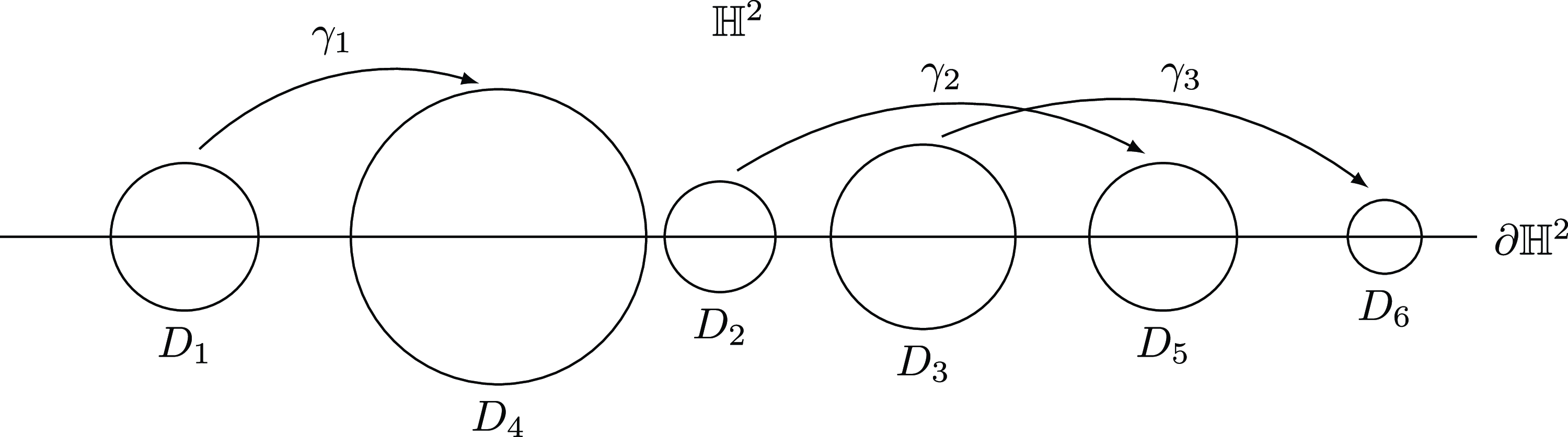
A configuration of Schottky disks and isometries with
 $ m=3$
.

An example configuration of Schottky disks and corresponding isometries is depicted in Figure 3.
Throughout the rest of this paper,
 $\Gamma$
is a non-elementary Schottky group with Schottky data
 $D_1, \ldots , D_{2m}$
and
 $\gamma _1, \ldots , \gamma _{2m}$
as above. This assumption will not be repeated in the sequel.
2.7. Combinatorial notation for words
Let
 $\Gamma$
be a Schottky group as in Section 2.6. We will follow the combinatorial notation of Dyatlov–Zworski [Reference Dyatlov and Zworski9] for indexing elements in the free group
 $\Gamma$
.
-
• A word
$\textbf {a}$
in the alphabet
$\mathcal{A} =\{ 1,\ldots ,2m \}$
is a finite string
$\textbf {a}=a_1 \ldots a_n$
with
$a_1, \ldots , a_n \in \mathcal{A}$
. For technical reasons, we also introduce the empty word
$\emptyset$
, a string of length zero. -
• A word
$\textbf {a}=a_1 \ldots a_n$
is said to be “reduced” if
$a_{j} \neq \overline {a_{j+1}}$
for all
$j=1,\ldots , n-1$
. For all
$n\in \mathbb{N}$
denote by
$\mathcal{W}_n$
the set of (reduced) words of length
$ n$
:Moreover, put
\begin{equation*} \mathcal{W}_n = \left \{ a_1\cdots a_n : \text{$a_1, \ldots , a_n \in \mathcal{A}$ s.t. $a_{j} \neq \overline {a_{j+1}} $ for all $j=1,\ldots , n-1$} \right \}. \end{equation*}
$ \mathcal{W}_0 = \{ \emptyset \}$
where
$ \emptyset$
is the empty word.
-
• Let
$ \mathcal{W} = \bigsqcup _{n\geqslant 0} \mathcal{W}_n$
be the set of all reduced words and write
$ \vert \textbf {a}\vert = n$
if
$ \textbf {a}\in \mathcal{W}_n$
. In other words,
$\vert \textbf {a}\vert$
is the reduced word length of
$\textbf {a}$
. Given
$m\in \mathbb{N}$
let
$\mathcal{W}_{\geqslant m} = \bigsqcup _{n\geqslant m} \mathcal{W}_n$
be the set of all reduced words whose length is at least
$m$
, and let
$ \mathcal{W}^\circ = \mathcal{W}_{\geqslant 1}$
be the set of all non-empty reduced words. -
• Given a word
$ \textbf {a} = a_1\cdots a_n \in \mathcal{W}^\circ$
write
$ \textbf {a}' = a_1\cdots a_{n-1} \in \mathcal{W}$
. Note that
$ \mathcal{W}$
is a tree with root
$ \emptyset$
and
$ \textbf {a}'$
is the parent of
$ \textbf {a}.$
-
• For
$ \textbf {a} = a_1\cdots a_n \in \mathcal{W}$
and
$ \textbf {b} = b_1\cdots b_m \in \mathcal{W}$
, write
$ \textbf {a}\to \textbf {b}$
if either
$ \textbf {a}= \emptyset$
, or
$ \textbf {b}= \emptyset$
, or
$ a_n \neq \overline {b_1}$
. Note that in this case,
$ \textbf {a}\textbf {b} \in \mathcal{W}$
, that is, if
$ \textbf {a}\to \textbf {b}$
, then the concatenation
$\textbf {a}\textbf {b}$
is also a reduced word. -
• Given a word
$\textbf {a} = a_1\cdots a_n$
, let
$\overline {\textbf {a}} = \overline {a_n}\cdots \overline {a_1}$
be its “mirror” word. -
• Write
$ \textbf {a}\prec \textbf {b}$
if
$ \textbf {a}$
is a prefix
$ \textbf {b}$
, that is, if
$ \textbf {b} = \textbf {ac}$
for some
$ \textbf {c}\in \mathcal{W}$
. -
• There is a one-to-one correspondence between reduced words
$\textbf {a} = a_1\cdots a_n \in \mathcal{W}$
and elements
$\gamma _{\textbf {a}} = \gamma _{a_1}\cdots \gamma _{a_n} \in \Gamma .$
Moreover, we have
$ \gamma _{\textbf {ab}} = \gamma _{\textbf {a}} \gamma _{\textbf {b}}$
,
$ \gamma _{\textbf {a}}^{-1} = \gamma _{\overline {\textbf {a}}}$
, and
$\gamma _{\textbf {a}} = I$
if and only if
$ \textbf {a} = \emptyset .$
-
• For
$ \textbf {a} = a_1 \cdots a_n \in \mathcal{W}^\circ$
, we define the diskIf
\begin{equation*} D_{\textbf {a}}\,:\!=\,\gamma _{\textbf {a}'}(D_{a_n}). \end{equation*}
$ \textbf {a}\prec \textbf {b}$
, then
$ D_{\textbf {b}}\subset D_{\textbf {a}}$
. On the other hand, if
$ \textbf {a}\nprec \textbf {b}$
and
$ \textbf {b}\nprec \textbf {a}$
, then
$ D_{\textbf {a}}\cap D_{\textbf {b}} = \emptyset$
. We also define the real interval(24)and we denote by
\begin{equation} I_{\textbf {a}} \,:\!=\, D_{\textbf {a}}\cap \mathbb{R} \end{equation}
$ \vert I_{\textbf {a}}\vert$
its length which is equal to the diameter of
$ D_{\textbf {a}}.$
The following uniform contraction property holds true: there are constants
$C\gt 0$
and
$0 \lt \alpha \lt 1$
such that for all
$\textbf {a}\in \mathcal{W}^\circ$
(25)see also Lemma 2.4 below.
\begin{equation} \vert I_{\textbf {a}}\vert \leqslant C \alpha ^{\vert \textbf {a}\vert }, \end{equation}
-
• Denote
\begin{equation*} \text{$D = \bigsqcup _{a\in \mathcal{A}} D_a $ and $ I = \bigsqcup _{a\in \mathcal{A}} I_a$.} \end{equation*}
-
• In the above notation, the limit set of
$\Gamma$
may be re-expressed as follows:
\begin{equation*} \Lambda = \bigcap _{n\geqslant 1} \bigsqcup _{\textbf {a}\in \mathcal{W}_n} I_{\textbf {a}} \subset \mathbb{R}. \end{equation*}
























2.8. Twisted transfer operators
In what follows, let
 $V$
be a finite-dimensional complex vector space with hermitian inner product
 $\langle \cdot ,\cdot \rangle _V$
and induced norm
 $\Vert v\Vert _V = \sqrt {\langle v,v\rangle _V}.$
Let
 $\rho \colon \Gamma \to \mathrm{U}(V)$
be a unitary representation. Recall that a representation is unitary if for any element
 $\gamma \in \Gamma$
and all vectors
 $ v,w\in V$
, one has
 $\langle \rho (\gamma )v,\rho (\gamma )w\rangle _V = \langle v,w\rangle _V$
and in particular
 $\Vert \rho (\gamma )v\Vert _V = \Vert v\Vert _V$
.
Let
 $H^2(D,V)$
be the Hilbert space of
 $V$
-valued, square-integrable, holomorphic functions on
 $D = \bigsqcup _{a\in \mathcal{A}} D_a$
:
 \begin{equation} H^2(D,V) \stackrel {\text{def}}{=} \left \{ \text{$f\colon D\to V$ holomorphic} \left \vert \; \left \Vert f \right \Vert \lt \infty \right .\right \}, \end{equation}
with
 $L^2$
-norm given by
 \begin{equation*} \Vert f\Vert ^2 \stackrel {\text{def}}{=} \int _D \Vert f(z)\Vert _V^2 \textrm {dvol}(z). \end{equation*}
Here, “
 $\textrm {vol}$
” denotes the Lebesgue measure on the complex plane. On this space, we define for all
 $s\in \mathbb{C}$
the twisted transfer operator
 \begin{equation} \mathcal{L}_{s,\rho }\colon H^2(D,V) \to H^2(D,V) \end{equation}
by the formula
 \begin{equation} \mathcal{L}_{s,\rho }f(z) \stackrel {\text{def}}{=} \sum _{\substack { a \in \mathcal{A} \\ a\to b }} \gamma _a'(z)^s \rho (\gamma _a)^{-1} f(\gamma _a (z))\ \mathrm{if}\ z\in D_b. \end{equation}
Since the derivative on the right satisfies
 $\gamma _a'(z)\gt 0$
for all
 $z\in I_b = D_b\cap {\mathbb{R}}$
, the complex power
 $\gamma _a'(z)^s$
is uniquely defined and holomorphic for
 $z\in D_b$
and
 $s\in \mathbb{C}.$
More concretely, we define
 \begin{equation*} \gamma _a'(z)^s \stackrel {\text{def}}{=} \exp ( s \mathbb{L}(\gamma _a'(z)) ), \end{equation*}
with
 \begin{equation} \mathbb{L}(z) = \log \vert z\vert + \mathrm{arg}(z), \end{equation}
where
 $\mathrm{arg}\colon \mathbb{C}\smallsetminus (\!-\infty , 0] \to (\!-\pi ,\pi )$
is the principal value of the argument.
We note that if
 $(\rho ,V) = (\textbf {1}_\Gamma ,\mathbb{C})$
is the trivial, one-dimensional representation,
 $H^2(\Omega ,V)$
reduces to the classical Bergman space
 $H^2(D)$
. Moreover, the operator in (27) reduces to the standard transfer operator
 $\mathcal{L}_s$
, which can be found for instance in Borthwick’s book [Reference Borthwick1, Chapter 15]. This operator is trace class for every
 $s\in \mathbb{C}$
and its Fredholm determinant is equal to the twisted Selberg zeta function of the Schottky group
 $\Gamma$
:
 \begin{equation} Z_{\Gamma }(s,\rho ) = \det (1-\mathcal{L}_{s,\rho }). \end{equation}
A proof of this identity for general twists can be found in [Reference Jakobson, Naud and Soares21]. Since
 $\mathcal{L}_{s,\rho }$
depends holomorphically on the variable
 $s\in \mathbb{C}$
, this identity shows that
 $Z_{\Gamma }(s,\rho )$
extends to an entire function.
2.9. Partitions and refined transfer operators
We now define the so-called refined transfer operators which were introduced by Dyatlov–Zworski [Reference Dyatlov and Zworski9]. These are generalizations of the standard transfer operator
 $\mathcal{L}_{s}$
. Given a finite subset
 $Z\subset \mathcal{W}$
, let
-
•
$Z'=\{ \textbf {a}' : \textbf {a}\in Z \}$
and -
•
$\overline {Z} =\{ \overline {\textbf {a}} : \textbf {a}\in Z \}.$


For any
 $s\in \mathbb{C}$
and any finite-dimensional unitary representation
 $\rho \colon \Gamma \to \mathrm{U}(V)$
, we define the operator
 \begin{equation} \mathcal{L}_{Z,s,\rho }\colon H^2(D,V) \to H^2(D,V) \end{equation}
by the formula
 \begin{equation} \mathcal{L}_{Z,s,\rho }f(z) \stackrel {\text{def}}{=} \sum _{\substack { \textbf {a}\in (\overline {Z})' \\ \textbf {a}\to b}} \gamma _{ \textbf {a}}'(z)^s \rho ( \gamma _{ \textbf {a}})^{-1} f( \gamma _{ \textbf {a}} (z))\ \mathrm{if}\ z\in D_b. \end{equation}
Note that
 $\mathcal{L}_{Z,s,\rho }=\mathcal{L}_{s,\rho }$
for
 $Z=\mathcal{W}_2$
, the set of reduced words of length two.
Definition 2.1 (Partitions). A finite set
 $Z\subset \mathcal{W}^\circ$
is called a partition if there is some
 $N\in \mathbb{N}$
with the following property: for every reduced word
 $\textbf {a}\in \mathcal{W}$
with
 $\vert \textbf {a}\vert \geqslant N$
, there exists a unique
 $\textbf {b}\in Z$
such that
 $\textbf {b}\prec \textbf {a}$
.
In terms of the limit set, a finite set
 $Z\subset \mathcal{W}^\circ$
is a partition if we have the disjoint union
 \begin{equation*} \Lambda = \bigsqcup _{\textbf {b}\in Z} ( I_{\textbf {b}} \cap \Lambda ). \end{equation*}
Recall that
 $\mathcal{W}_n$
denotes the set of reduced words of length
 $n$
. The sets
 $\mathcal{W}_n$
for
 $n\geqslant 2$
are trivial examples for partitions and, in this case, we have
 $\mathcal{L}_{\mathcal{W}_n,s} = \mathcal{L}_s^{n-1}.$
The fundamental fact about partitions is the following result:
Lemma 2.2.
Let
 $Z \subset \mathcal{W}_{\geqslant 2}$
be a partition. There exists a holomorphic family of trace class operators
 $T_{Z,s,\rho }$
such that
 \begin{equation} 1-\mathcal{L}_{Z,s,\rho } = (1+T_{Z,s,\rho })(1-\mathcal{L}_{s,\rho }). \end{equation}
In particular, we have
 \begin{equation} \det (1-\mathcal{L}_{Z,s,\rho } )= \det (1+T_{Z,s,\rho }) Z_\Gamma (s,\rho ). \end{equation}
Remark 2.3.
Lemma 2.2 extends Lemma 2.4 in the paper of Dyatlov–Zworski [Reference Dyatlov and Zworski9], which states that any
 $1$
-eigenfunction of the standard transfer operator
 $\mathcal{L}_{s}$
is also a 1-eigenfunction for
 $\mathcal{L}_{Z,s}$
. Lemma 2.2
, however, goes further by asserting that the Fredholm determinant
 $\det \left ( 1 - \mathcal{L}_{\tau ,s,\rho } \right )$
is a holomorphic multiple of
 $Z_\Gamma (s,\rho )$
. Consequently, the zeros of the Selberg zeta function appear with at least the same multiplicity as the zeros of
 $\det \left ( 1 - \mathcal{L}_{\tau ,s,\rho } \right )$
. Fortunately, to prove Lemma 2.2
, we only need to make slight modifications to the original proof from [Reference Dyatlov and Zworski9].
Proof.
First note that the identity in (34) follows from taking determinants on both sides of (33) and then applying (30). Thus, we only need to prove (33). We argue by induction on
 $\sum _{\textbf {b}\in Z'} \vert \textbf {b}\vert$
. If
 $Z = \mathcal{W}_2$
, then
 $\mathcal{L}_{Z,s,\rho } = \mathcal{L}_{s,\rho }$
, so (33) holds true with
 $T_{\mathcal{W}_2,s,\rho } = 0$
. If
 $Z \neq \mathcal{W}_2$
, choose a word
 $\textbf {d}c\in Z$
of maximal length, where
 $\textbf {d}\in \mathcal{W}^\circ$
and
 $c\in \mathcal{A}$
.
Then
 $Z$
has the form (see Figure 4)
 \begin{equation} Z = (Z_0 \smallsetminus \{ \textbf {d} \}) \sqcup \{ \textbf {d}a \,:\, a\in \mathcal{A}, \textbf {d}\to a \}, \end{equation}
where
 $Z_0$
is a partition containing
 $\textbf {d}$
. By the inductive hypothesis, we have
 \begin{equation} 1-\mathcal{L}_{Z_0,s,\rho } = (1+T_{Z_0,s,\rho })(1-\mathcal{L}_{s,\rho }). \end{equation}
Observe that we can write
 \begin{equation*} \mathcal{L}_{Z,s,\rho } = \sum _{\textbf {a}\in (\overline {Z})'} \nu _{\textbf {a},s,\rho }, \end{equation*}
where
 $\nu _{\textbf {a},s,\rho }\colon H^2(D,V)\to H^2(D,V)$
is the trace class operator defined by
 \begin{equation*} \nu _{\textbf {a},s,\rho }(f)(z) = \begin{cases} \rho (\gamma _{\textbf {a}})^{-1}\gamma _{\textbf {a}}'(z)^s f(\gamma _{\textbf {a}} (z)) &\text{if $\textbf {a}\to z$}\\ 0 &\text{else}. \end{cases}. \end{equation*}
It follows from (35) that
 \begin{equation} \mathcal{L}_{Z,s,\rho } = \mathcal{L}_{Z_0 \smallsetminus \{ \textbf {d} \},s,\rho } + \sum _{a\in \mathcal{A}} \nu _{\overline {\textbf {d}a}', s,\rho }. \end{equation}
Note that for any
 $a\in \mathcal{A}$
such that
 $\textbf {d}\to a$
, we have the rule
 $\overline {\textbf {d}a}' = \overline {a} \overline {\textbf {d}}'$
. Applying the chain rule yields
 \begin{equation*} \nu _{\overline {\textbf {d}a}',s, \rho } = \nu _{\overline {\textbf {d}}',s,\rho } \nu _{a,s,\rho }. \end{equation*}
Inserting this into (37), we get
 \begin{align*} \mathcal{L}_{Z,s,\rho } &= \mathcal{L}_{Z_0 \smallsetminus \{ \textbf {d} \},s,\rho } + \sum _{a\in \mathcal{A}} \nu _{\overline {\textbf {d}}', s,\rho } \nu _{a,s,\rho }\\ &= \mathcal{L}_{Z_0,s,\rho } - \nu _{\overline {\textbf {d}}', s,\rho } + \nu _{\overline {\textbf {d}}', s,\rho } \mathcal{L}_{s,\rho } \\ &= \mathcal{L}_{Z_0,s,\rho } - \nu _{\overline {\textbf {d}}', s,\rho } (1-\mathcal{L}_{s,\rho }). \end{align*}
Together with (36), we now obtain
 \begin{equation*} 1-\mathcal{L}_{Z,s,\rho } = 1- \mathcal{L}_{Z_0,s,\rho } + \nu _{\overline {\textbf {d}}', s,\rho } (1-\mathcal{L}_{s,\rho }) = (1+T_{Z_0,s,\rho } + \nu _{\overline {\textbf {d}}', s,\rho })(1-\mathcal{L}_{s,\rho }). \end{equation*}
This proves (33) with
 \begin{equation*} T_{Z,s,\rho } \stackrel {\text{def}}{=} T_{Z_0,s,\rho } + \nu _{\overline {\textbf {d}}', s,\rho }. \end{equation*}
Recall that the sum of trace class operators remains trace class. In particular,
 $T_{Z,s,\rho }$
is trace class. That
 $T_{Z,s,\rho }$
is a holomorphic family in
 $s\in {\mathbb{C}}$
follows by a similar reasoning. The proof is finished.
An example of a partition
 $Z$
, with elements of
 $Z$
shaded gray in the tree of words
 $\mathcal{W}$
in the alphabet
 $\mathcal{A} = \{ 1,2,3,4 \}$
. The solid black word is one possible choice of
 $\textbf {d}$
in the proof of Lemma 2.2.

Let us now introduce the partitions relevant in this paper, again following [Reference Dyatlov and Zworski9]. For any sufficiently small
 $\tau \gt 0$
, called the resolution parameter, we define
 \begin{equation} Z(\tau ) \stackrel {\text{def}}{=} \left \{ \mathbf{a} \in \mathcal{W}^{\circ } : |I_{\mathbf{a}}| \leqslant \tau \lt |I_{\mathbf{a}'}| \right \}. \end{equation}
The set
 $Z(\tau )$
is a partition by virtue of (25). We now define the
 $\tau$
-refined transfer operator by
 \begin{equation} \mathcal{L}_{\tau ,s,\rho } \stackrel {\text{def}}{=} \mathcal{L}_{Z(\tau ),s,\rho }. \end{equation}
By Equation (32), the operator
 $\mathcal{L}_{\tau ,s,\rho }$
is explicitly defined as follows: for each
 $f\in H^2(D,V)$
and each fixed
 $b\in \mathcal{A}$
, we put for all
 $z\in D_b$
,
 \begin{equation} \mathcal{L}_{\tau ,s,\rho } f(z) = \sum _{\substack { \textbf {a}\in Y(\tau ) \\ \textbf {a}\to b}} \gamma _{ \textbf {a}}'(z)^s \rho (\gamma _{ \textbf {a}})^{-1} f(\gamma _{ \textbf {a}}(z)) \end{equation}
where
 \begin{equation} Y(\tau ) \stackrel {\text{def}}{=} \overline {Z(\tau )}'. \end{equation}
Note that the operator (39) is well-defined as long as
 $Y(\tau )\subset W^\circ$
, or equivalently,
 $Z(\tau )\subset W_{\geqslant 2}$
. This condition holds true once
 $\tau \gt 0$
is small enough, see Lemma 2.7 below.
We use this specific family of operators because it allows us to control both the size of
 $Y(\tau )$
as well as the size of the derivatives
 $\gamma _{\textbf {a}}'$
when
 $\textbf {a}\in Y(\tau )$
, see Lemma 2.7 below.
2.10. Some useful bounds for Schottky groups
We now record some useful estimates for Schottky groups when acting on the hyperbolic plane. The following basic estimates are due to Naud [Reference Naud29]:
Lemma 2.4 (Basic distortion estimates). The following estimates hold true with implied constants depending only on
 $\Gamma$
:
-
(1) Uniform contraction: There are constants
$ 0 \lt \theta _1 \lt \theta _2 \lt 1$
such that for all
$ b\in \mathcal{A}$
and
$ \textbf {a}\in \mathcal{W}$
with
$ \textbf {a}\to b$
and
$ z\in D_b$
we have
\begin{equation*} \theta _1^{\vert \textbf {a}\vert } \ll _\Gamma \vert \gamma _{\textbf {a}}'(z)\vert \ll _\Gamma \theta _2^{\vert \textbf {a}\vert }. \end{equation*}
-
(2) Bounded distortion 1: For all
$ b\in \mathcal{A}$
and
$ \textbf {a}\in \mathcal{W}$
with
$ \textbf {a}\to b$
and
$ z_1, z_2\in D_b$
we have
\begin{equation*} \vert \gamma _{\textbf {a}}'(z_1)\vert \asymp _\Gamma \vert \gamma _{\textbf {a}}'(z_2)\vert , \end{equation*}
-
(3) Bounded distortion 2: For all
$ b_1,b_2\in \mathcal{A}$
, all
$z_1\in D_{b_1}$
, and all
$z_2\in D_{b_2}$
, and all
$\textbf {a}\in \mathcal{W}^\circ$
with
$\textbf {a}\to b_1,b_2$
, we have
\begin{equation*} \vert \gamma '_{\textbf {a}}(z_1)\vert \asymp _\Gamma \vert \gamma '_{\textbf {a}}(z_2)\vert . \end{equation*}


We now introduce additional notations, following Magee–Naud [Reference Naud and Magee30]. For every
 $a\in \mathcal{A}$
, choose a point
 $o_a \in I_a$
. From now on, we view these points as fixed. For any
 $\textbf {a}\in \mathcal{W}^\circ$
, we define
 \begin{equation*} o_{\textbf {a}} \stackrel {\text{def}}{=} o_b \end{equation*}
for some
 $b\in \mathcal{A}$
such that
 $\textbf {a}\to b$
, and we let
 $o_\emptyset$
be some arbitrary point in
 $D$
. Next, for any
 $\textbf {a}\in \mathcal{W}$
we define
 \begin{equation*} \Upsilon _{\textbf {a}} \stackrel {\text{def}}{=} \gamma _{\textbf {a}}'(o_{\textbf {a}}). \end{equation*}
As it turns out, the derivatives
 $\gamma _{\textbf {a}}'(z)$
for any
 $z\in D_b$
, where
 $b\in \mathcal{A}$
is such that
 $\textbf {a}\to b$
, are all comparable to
 $\Upsilon _{\textbf {a}}$
in a uniform way. We have the following estimates from [Reference Naud and Magee30]:
Lemma 2.5 (Bounds for derivatives). The following estimates hold true with implied constants depending solely upon
 $\Gamma$
:
-
(1) For all
$b\in \mathcal{A}$
and
$z\in D_b$
with
$\textbf {a}\to b$
, we have
$\vert \gamma '_{\textbf {a}}(z)\vert \asymp \Upsilon _{\textbf {a}}$
. -
(2) For all
$\textbf {a}\in \mathcal{W}^\circ$
, we have
$\Upsilon _{\textbf {a}'} \asymp \Upsilon _{\textbf {a}}$
. -
(3) For all
$\textbf {a}\in \mathcal{W}^\circ$
, we have
$\Upsilon _{\overline {\textbf {a}}} \asymp \Upsilon _{\textbf {a}}$
. -
(4) For all
$\textbf {a},\textbf {b}\in \mathcal{W}^\circ$
with
$\textbf {a}\to \textbf {b}$
, we have
$\Upsilon _{\textbf {a}\textbf {b}} \asymp \Upsilon _{\textbf {a}} \Upsilon _{\textbf {b}}.$


Combining Lemma 2.4 and Lemma 2.5 yields
Lemma 2.6 (Complex powers of derivatives). For all
 $b\in \mathcal{A}$
,
 $\textbf {a}\in \mathcal{W}^\circ$
with
 $\textbf {a}\to b$
,
 $z\in D_b$
, and
 $s=\sigma +it$
with
 $\sigma \gt 0$
, we have
 \begin{equation*} \vert \gamma _{\textbf {a}}'(z)^s\vert \ll (C \Upsilon _{\textbf {a}})^\sigma e^{C\vert t\vert }, \end{equation*}
where
 $C\gt 0$
and the implied constant depend solely on
 $\Gamma$
.
Recall the definitions of the sets
 $Z(\tau )$
and
 $Y(\tau )$
in (38) and (41), respectively. Also crucial are the following estimates:
Lemma 2.7 (Estimates concerning
 $Z(\tau )$
and
 $Y(\tau )$
). For all
 $\tau \gt 0$
small enough the following estimates hold true with implied constants depending only on
 $\Gamma$
:
-
(1) For all
$ \textbf {a}\in Z(\tau )$
, we have
$\Upsilon _{\textbf {a}} \asymp \tau .$
-
(2) For all
$ \textbf {a}\in Y(\tau )$
, we have
$\Upsilon _{\textbf {a}} \asymp \tau .$
-
(3)
$ \vert Y(\tau )\vert \asymp \vert Z(\tau )\vert \asymp \tau ^{-\delta }.$
-
(4) For all
$\textbf {a}\in Y(\tau )$
, we have
$\vert \textbf {a}\vert \asymp \log (\tau ^{-1}).$
-
(5) For all
$\textbf {a}\in Y(\tau )$
, we have
$\Vert \gamma _{\textbf {a}}\Vert \asymp \tau ^{-1/2}$
, where
$\Vert \cdot \Vert$
denotes the Frobenius norm:
\begin{equation*} \left \Vert \begin{pmatrix} a& \,\,b\\c&\,\,d\end{pmatrix} \right \Vert = \sqrt {a^2 + b^2 + c^2 + d^2}. \end{equation*}





Proof.
The estimates for
 $Z(\tau )$
can be found in [Reference Bourgain and Dyatlov3]. It is straightforward to deduce the corresponding estimates for
 $Y(\tau )$
, using those for
 $Z(\tau )$
and Lemma 2.5. Moreover, Part (4) corresponds to [Reference Naud and Magee30, Lemma 3.3] while Part (5) follows from [Reference Calderón and Magee7, Lemma 10].
2.11. Hilbert–Schmidt norm of refined transfer operators
Given a trace class operator
 $A\colon H\to H$
on a separable Hilbert space
 $H$
, the Hilbert–Schmidt norm is defined by
 \begin{equation} \Vert A\Vert _{\mathrm{HS}}^2 \stackrel {\text{def}}{=} \mathrm{tr} \left ( A A^{\ast } \right ), \end{equation}
where
 $A^{\ast }$
denotes the adjoint of
 $A$
. The goal of this subsection is to prove
Lemma 2.8 (HS-norm). For any finite-dimensional unitary representation
 $\rho \colon \Gamma \to \mathrm{U}(V)$
, the Hilbert–Schmidt norm of the operator
 $\mathcal{L}_{\tau ,s,\rho }$
is given by the formula
 \begin{equation} \Vert \mathcal{L}_{\tau ,s,\rho } \Vert _{\mathrm{HS}}^2 = \sum _{b\in \mathcal{A}}\sum _{\substack { \textbf {a},\textbf {b}\in Y(\tau ) \\ \textbf {a},\textbf {b}\to b }} \mathrm{tr} \left ( \rho (\gamma _{\textbf {a}}^{-1} \gamma _{\textbf {b}}) \right ) \mathcal{I}_{\textbf {a},\textbf {b}}^{(b)}, \end{equation}
where
 \begin{equation} \mathcal{I}_{\textbf {a},\textbf {b}}^{(b)} = \int _{D_b} \gamma '_{\textbf {a}}(z)^s \overline {\gamma '_{\textbf {b}}(z)^s } B_D(\gamma _{\textbf {a}}(z), \gamma _{\textbf {b}}(z))\, \textrm {dvol}(z). \end{equation}
Here,
 $B_{D}(z,w)$
is the reproducing kernel of the Bergman space
 $H^2(D).$
Moreover, for all
 $\sigma_0 \gt 0$
, for all
 $s = \sigma + it$
with
 $\sigma \geqslant \sigma_0$
, for all
 $b\in \mathcal{A}$
and for all
 $\textbf {a},\textbf {b}\in Y(\tau )$
with
 $\textbf {a},\textbf {b}\to b$
, we have the bound
 \begin{equation} \vert \mathcal{I}_{\textbf {a},\textbf {b}}^{(b)}\vert \ll _\Gamma (C\tau )^{2\sigma_0} e^{C \vert t\vert }, \end{equation}
for some constant
 $C=C(\Gamma )\gt 0$
.
Proof.
Formulas for the HS-norm of similar operators are given in [Reference Naud and Magee30, Lemma 4.7] and in [Reference Pohl and Soares34, Proposition 5.5]. We will provide an alternative but essentially equivalent argument. We denote by
 $B_D(z,w)$
the reproducing kernel of the classical Bergman space
 $H^2(D)$
over
 $D = \bigsqcup _{b\in \mathcal{A}} D_b$
. This kernel satisfies
 $\overline {B_{D}(\cdot ,w)}\in H^2(D)$
for all
 $w\in D$
and
 \begin{equation*} \int _{D} B_{D}(z,w) f(w) \textrm {dvol}(w) = f(z) \end{equation*}
for all
 $f\in H^2(D)$
and all
 $z\in D$
, and is uniquely defined by these two properties. Hence, using the formula in (40),
 $\mathcal{L}_{\tau ,s,\rho }$
can be rewritten as the integral operator
 \begin{equation*} \mathcal{L}_{\tau ,s,\rho } f(z) = \int _D K_{\tau ,s,\rho }(z,w) f(w)\textrm {dvol}(w), \end{equation*}
where the kernel is given for all
 $z,w\in D$
by
 \begin{equation*} K_{\tau ,s,\rho }(z,w) = \sum _{\substack { \textbf {a}\in Y(\tau ) \\ \textbf {a}\to b }} \gamma '_{\textbf {a}}(z)^s \rho (\gamma _{\textbf {a}})^{-1} B_D(\gamma _{\textbf {a}}(z),w), \quad \text{if $z\in D_b$.} \end{equation*}
Note that if the points
 $z,w\in D$
are fixed, then
 $K_{\tau ,s,\rho }(z,w)$
is an element of the endomorphism ring
 $\mathrm{End}(V)$
of
 $V$
. The Hilbert–Schmidt norm on
 $\mathrm{End}(V)$
is defined by
 \begin{equation*} \Vert A\Vert _2 = \sqrt {\mathrm{tr}_V(A A^\ast )}, \quad A\in \mathrm{End}(V), \end{equation*}
where
 $\mathrm{tr}_V$
is the trace of
 $V$
. We will drop the subscript
 $V$
from the notation, writing only
 $\mathrm{tr}_V = \mathrm{tr}$
. Hence, the Hilbert–Schmidt norm of
 $K_{\tau ,s,\rho }(z,w)$
(when viewed as an element of
 $\mathrm{End}(V)$
) is given by
 \begin{align*} \Vert K_{\tau ,s,\rho }(z,w)\Vert _2^2 &= \textrm {tr}\left ( K_{\tau ,s,\rho }(z,w) K_{\tau ,s,\rho }(z,w)^\ast \right )\\ &= \sum _{\substack { \textbf {a},\textbf {b}\in Y(\tau ) \\ \textbf {a},\textbf {b}\to b }} \mathrm{tr} \left ( \rho (\gamma _{\textbf {a}}^{-1} \gamma _{\textbf {b}}) \right ) \gamma '_{\textbf {a}}(z)^s \overline {\gamma '_{\textbf {b}}(z)^s } B_D(\gamma _{\textbf {a}}(z),w) \overline {B_D(\gamma _{\textbf {b}}(z),w)}. \end{align*}
Note that for the second equality, we used the linearity of the trace and the rule
 $ \rho (\gamma _{\textbf {a}})^\ast \rho ( \gamma _{\textbf {b}}) = \rho (\gamma _{\textbf {a}}^{-1} \gamma _{\textbf {b}}),$
which follows from the unitarity of the representation
 $\rho$
. The Hilbert–Schmidt norm of
 $\mathcal{L}_{\tau ,s,\rho }$
can now be computed as
 \begin{align*} \Vert \mathcal{L}_{\tau ,s,\rho } \Vert _{\mathrm{HS}}^2 &= \int _D \int _D \Vert K_{\tau ,s,\rho }(z,w)\Vert _2^2 \textrm {dvol}(w)\textrm {dvol}(z)\\ &= \sum _{b\in \mathcal{A}} \int _{D_b} \int _D \Vert K_{\tau ,s,\rho }(z,w)\Vert _2^2 \textrm {dvol}(w)\textrm {dvol}(z)\\ &= \sum _{b\in \mathcal{A}} \sum _{\substack { \textbf {a},\textbf {b}\in Y(\tau ) \\ \textbf {a},\textbf {b}\to b }} \mathrm{tr} \left ( \rho (\gamma _{\textbf {a}}^{-1} \gamma _{\textbf {b}}) \right ) \mathcal{I}_{\textbf {a},\textbf {b}}^{(b)}, \end{align*}
where, in the last line, we put
 \begin{equation} \mathcal{I}_{\textbf {a},\textbf {b}}^{(b)} \stackrel {\text{def}}{=} \int _{D_b} \gamma '_{\textbf {a}}(z)^s \overline {\gamma '_{\textbf {b}}(z)^s } \left ( \int _D B_D(\gamma _{\textbf {a}}(z),w) \overline {B_D(\gamma _{\textbf {b}}(z),w)} \textrm {dvol}(w) \right )\textrm {dvol}(z). \end{equation}
By the defining property of the Bergman kernel, we have
 \begin{align*} \int _D B_D(\gamma _{\textbf {a}}(z),w) \overline {B_D(\gamma _{\textbf {b}}(z),w)}\, \textrm {dvol}(w) &= \int _D B_D(\gamma _{\textbf {a}}(z),w) B_D(w,\gamma _{\textbf {b}}(z)) \,\textrm {dvol}(w) \\ &= B_D(\gamma _{\textbf {a}}(z), \gamma _{\textbf {b}}(z)), \end{align*}
which when inserted into (46) yields
 \begin{equation*} \mathcal{I}_{\textbf {a},\textbf {b}}^{(b)} = \int _{D_b} \gamma '_{\textbf {a}}(z)^s \overline {\gamma '_{\textbf {b}}(z)^s } B_D(\gamma _{\textbf {a}}(z), \gamma _{\textbf {b}}(z))\, \textrm {dvol}(z), \end{equation*}
as claimed in (44).
Let us now prove the bound in (45). Fix
 $b\in \mathcal{A}$
and
 $\textbf {a},\textbf {b}\in Y(\tau )$
so that
 $\textbf {a},\textbf {b}\to b$
. Combining Lemmas 2.6 and 2.7 implies that for all
 $z\in D_b,$
 \begin{equation*} \vert \gamma _{\textbf {a}}'(z)^{s}\vert \ll (C \tau)^{\sigma } e^{C \vert t\vert} \leqslant (C \tau)^{\sigma_0} e^{C \vert t\vert}\end{equation*}
for some constant
 $C=C(\Gamma )\gt 0$
, where for the second estimate we assume that
 $\tau \gt0$
is small enough so that
 $C\tau \leqslant 1$
. Thus, applying the triangle inequality, it follows that
 \begin{align*} \vert \mathcal{I}_{\textbf {a},\textbf {b}}^{(b)}\vert &\leqslant \int _{D_b} \vert \gamma _{\textbf {a}}'(z)^{s}\vert \vert \gamma _{\textbf {b}}'(z)^{s} \vert \vert B_D(\gamma _{\textbf {a}}(z), \gamma _{\textbf {b}}(z)) \vert \textrm {dvol}(z)\\ &\ll (C\tau )^{2\sigma_0 } e^{2C \vert t\vert } \sup _{z\in D_b} \vert B_D(\gamma _{\textbf {a}}(z), \gamma _{\textbf {b}}(z)) \vert . \end{align*}
It remains to prove that
 \begin{equation} \sup _{z\in D_b} \vert B_D(\gamma _{\textbf {a}}(z), \gamma _{\textbf {b}}(z)) \vert \ll _\Gamma 1. \end{equation}
Note that
 $B_D(z,w)$
equals zero unless the points
 $z$
and
 $w$
belong to the same Schottky disk
 $D_b$
, in which case
 $B_D(z,w) = B_{D_b}(z,w)$
. Let
 $r_b\gt 0$
and
 $c_b\in \mathbb{R}$
be the radius and the center of
 $D_b$
, respectively. We then have the following formula for the Bergman kernel over
 $D_b$
, see for instance [Reference Duren and Schuster8, Chapter 1]:
 \begin{equation*} B_{D_b}(z,w) = \frac {r_b^2}{\pi ^2 \left ( r_b^2 - (z-c_b)(\overline {w}-c_b) \right )^2}. \end{equation*}
Applying the elementary inequality
 $\vert R^2 - u v\vert ^2\geqslant R^2 (R-\vert u\vert ) (R-\vert v\vert )$
, valid for all
 $R\gt 0$
and all points
 $u,v\in {\mathbb{C}}$
with
 $\vert u\vert , \vert v\vert \leqslant R$
, we find
 \begin{align*} \vert r_b^2 - (z-c_b)(\overline {w}-c_b) \vert ^2 &\geqslant r_b^2 ( r_b-\vert z-c_b\vert ) (r_b-\vert w-c_b\vert )\\ &= r_b^2\, \textrm {dist}( z,\partial D_b )\, \textrm {dist}\,( w,\partial D_b ). \end{align*}
Here,
 $\textrm {dist}( \cdot ,\partial D_b )$
denotes the minimal euclidean distance to the boundary
 $\partial D_b$
. We deduce that
 \begin{equation} \vert B_{D_b}(z,w)\vert \ll \frac {1}{\textrm {dist}( z,\partial D_b ) \,\textrm {dist}( w,\partial D_b )}. \end{equation}
By the uniform contraction property from Lemma 2.4, there exists some
 $c = c(\Gamma )\gt 0$
such that for all
 $\textbf {a}\in \mathcal{W}^\circ$
with
 $\textbf {a}\to b$
, we have
 \begin{equation*} \textrm {dist}( \gamma _{\textbf {a}}(z),\partial D )\geqslant c. \end{equation*}
Inserting this into (48) yields the desired bound (47), completing the proof.
3. Counting zeros of Selberg zeta functions
For every finite-dimensional unitary representation
 $\rho$
of
 $\Gamma$
, let
 $N_\Gamma (\rho , \sigma )$
denote the number of zeros of
 $Z_{\Gamma }(s,\rho )$
in the interval
 $[\sigma ,\delta ]$
counted with multiplicities. The goal of this section is to prove.
Proposition 3.1 (Key zero counting result). Let
 $(\rho _j)_{j\in J}$
be a finite collection of finite-dimensional unitary representations of
 $\Gamma .$
Recall the definition of the HS-norm in
(42)
. Then, there are positive constants
 $\alpha , \beta ,\tau _0, K_0, C$
, depending only on
 $\Gamma$
, such that for all
 $0 \lt \tau \lt \tau _0$
and for all
 $K \gt K_0$
,
 \begin{equation*} \sum _{j\in J} N_\Gamma (\rho _j, \sigma ) \leqslant C K^2 \max _{\substack { \mathrm{Re}(s)\geqslant \sigma -\frac {\alpha }{K} \\ \vert \mathrm{Im}(s)\vert \leqslant \beta K }} \left ( \sum _{j\in J} \Vert \mathcal{L}_{\tau , s, \rho _j} \Vert _{\mathrm{HS}}^2 \right ) + \left ( \sum _{j\in J} \dim (\rho _j) \right ) K^2 (C\tau )^{2K}, \end{equation*}
where
 $\dim (\rho )$
denotes the dimension of the representation
 $\rho .$
Consider the refined zeta function
 \begin{equation*} \zeta _{\tau }(s,\rho ) \stackrel {\text{def}}{=} \det \left ( 1-\mathcal{L}_{\tau ,s,\rho }^{2} \right ) = \det \left ( 1-\mathcal{L}_{\tau ,s,\rho } \right ) \det \left ( 1+\mathcal{L}_{\tau ,s,\rho } \right ). \end{equation*}
By Lemma 2.2,
 $\zeta _{\tau }(s,\rho )$
is the product of the Selberg zeta function and an entire function. Consequently, an upper bound for
 $N_\Gamma (\rho , \sigma )$
can be obtained by estimating the number of zeros of
 $\zeta _{\tau }(s, \rho )$
within the interval
 $[\sigma , \delta ].$
First, we need the following:
Lemma 3.2 (Pointwise estimate for
 $\zeta _{\tau }(s,\rho )$
). There are
 $C\gt 0$
and
 $\tau _0 \gt 0$
, depending only on
 $\Gamma$
, such that for all
 $0\lt \tau \lt \tau _0$
and for all
 $s\in \mathbb{C}$
with
 $\sigma = \mathrm{Re}(s) \gt \delta$
, the following estimate holds:
 \begin{equation*} - \log \vert \zeta _{\tau }(s,\rho )\vert \leqslant \dim (\rho ) \frac {(C \tau )^{2(\sigma -\delta )}}{1-(C \tau )^{2(\delta -\sigma )}}. \end{equation*}
Proof.
Given a Hilbert space
 $H$
and a trace class operator
 $A\colon H\to H$
with
 $\Vert A\Vert _H \lt 1$
, we have the absolutely convergent series expansion
 \begin{equation} \det (1-A) = \exp \left ( -\sum _{k=1}^\infty \frac {1}{k} \mathrm{tr}(A^k) \right ), \end{equation}
see for instance [Reference Gohberg, Goldberg and Krupnik13]. Taking absolute values and logarithms on both sides yields
 \begin{equation} - \log \vert \det (1-A)\vert \leqslant \sum _{k=1}^\infty \frac {1}{k} \vert \mathrm{Re} (\mathrm{tr}(A^k)) \vert \leqslant \sum _{k=1}^\infty \frac {1}{k} \vert \mathrm{tr}(A^k) \vert . \end{equation}
Applying this to
 $A=\mathcal{L}_{\tau ,s,\rho }^{2}$
with
 $\sigma = \mathrm{Re}(s)\gt \delta$
gives
 \begin{equation} - \log \vert \zeta _{\tau }(s,\rho )\vert \leqslant \sum _{k=1}^\infty \frac {1}{k} \vert \mathrm{tr}(\mathcal{L}_{\tau ,s,\rho }^{2k})\vert . \end{equation}
From the proof of Proposition 4.8 in Magee–Naud [Reference Naud and Magee30], the traces on the right are bounded by
 \begin{equation*} \vert \mathrm{tr}( \mathcal{L}_{\tau ,s,\rho }^{2k} ) \vert \leqslant \dim (\rho ) (C \tau )^{2k \sigma } \vert Z(\tau )\vert ^{2k}, \end{equation*}
where
 $C\gt 0$
depends only on
 $\Gamma .$
By Lemma 2.7 we have
 \begin{equation*} \vert Z(\tau )\vert \ll \tau ^{-\delta }. \end{equation*}
Combining the previous two estimates yields (possibly with a larger constant
 $C$
)
 \begin{equation*} \vert \mathrm{tr}( \mathcal{L}_{\tau ,s,\rho }^{2k} ) \vert \leqslant \dim (\rho ) (C \tau )^{2k (\sigma -\delta )}. \end{equation*}
Returning to (51) and using the geometric series formula, we obtain for all sufficiently small
 $\tau \gt 0$
,
 \begin{equation*} - \log \vert \zeta _{\tau }(s,\rho )\vert \leqslant \dim (\rho ) \sum _{k=1}^\infty (C \tau )^{2k (\sigma -\delta )} = \dim (\rho ) \frac {(C \tau )^{2(\sigma -\delta )}}{1-(C \tau )^{2(\delta -\sigma )}}, \end{equation*}
as claimed.
We are now ready to give the
Proof of Proposition
3.1
. We will use essentially the same argument as in [Reference Jakobson and Naud20, Reference Pohl and Soares34]. We will use Jensen’s formula for holomorphic functions, or rather a weaker variant thereof, which we recall now. Consider an entire function
 $f$
and a pair of concentric disks
 $D_i = D_{\mathbb{C}}(\sigma _0, r_i)$
with
 $i\in \{1,2\}$
centered at
 $\sigma _0\in \mathbb{R}$
and with radii
 $r_2 \gt r_1 \gt 0$
. Assume that
 $\sigma _0, r_1, r_2$
are chosen such that
 \begin{equation} [\sigma ,\delta ]\subset \overline {D_1} \subset D_2. \end{equation}
Define the zero counting function
 \begin{equation*} M_f(\sigma ,\delta ) \stackrel {\text{def}}{=} \# \{ s \in \mathbb{C} : \text{$f(s)=0$, $s\in [\sigma ,\delta ]$} \}, \end{equation*}
where zeros are repeated according to multiplicity. Then, we have
 \begin{equation} M_f(\sigma ,\delta ) \leqslant \frac {1}{\log ( r_2/r_1 )} \left ( \int _{0}^{1} \log \vert f( \sigma _0 + r_2 e^{2\pi i \theta }) \vert d\theta - \log \vert f (\sigma _0)\vert \right ). \end{equation}
Applying this to the refined zeta function
 $f(s)=\zeta _{\tau }(s,\rho )$
(for any given finite-dimensional unitary representation
 $\rho$
) and recalling the remark preceding Lemma 3.2, we obtain
 \begin{equation} N_\Gamma (\rho , \sigma ) \leqslant \frac {1}{\log ( r_2/r_1 )} \left ( \int _{0}^{1} \log \vert \zeta _{\tau } ( \sigma _0 + r_2 e^{2\pi i \theta }, \rho ) \vert d\theta - \log \vert \zeta _{\tau } (\sigma _0, \rho )\vert \right ). \end{equation}
If we assume furthermore that
 $\sigma _0 \gt \delta$
, then we can apply the pointwise estimate in Lemma 3.2 to estimate
 \begin{equation} N_\Gamma (\rho , \sigma ) \leqslant \frac {1}{\log ( r_2/r_1 )} \left ( \int _{0}^{1} \log \vert \zeta _{\tau } ( \sigma _0 + r_2 e^{2\pi i \theta }, \rho ) \vert d\theta + \dim (\rho ) \frac {(C \tau )^{2(\sigma _0-\delta )}}{1-(C \tau )^{2(\sigma _0-\delta )}} \right ). \end{equation}
Next, using Weyl’s estimate
 \begin{equation*} \log \vert \det (1-A)\vert \leqslant \Vert A\Vert _1 \end{equation*}
together with the Cauchy–Schwarz-type bound
 \begin{equation*} \Vert A_1 A_2\Vert _{1} \leqslant \Vert A_1\Vert _{\mathrm{HS}}\Vert A_2\Vert _{\mathrm{HS}}, \end{equation*}
we obtain
 \begin{equation} \log \vert \zeta _{\tau } (s, \rho ) \vert \leqslant \Vert \mathcal{L}_{\tau , s, \rho}^2\Vert _{1} \leqslant \Vert \mathcal{L}_{\tau , s, \rho }\Vert _{\mathrm{HS}}^2. \end{equation}
Inserting this into (55) yields
 \begin{equation} N_\Gamma (\rho , \sigma ) \leqslant \frac {1}{\log ( r_2/r_1 )} \left ( \int _{0}^{1} \Vert \mathcal{L}_{\tau , \sigma _0 + r_2 e^{2\pi i \theta }, \rho } \Vert _{\mathrm{HS}}^2 d\theta + \dim (\rho ) \frac {(C \tau )^{2(\sigma _0-\delta )}}{1-(C \tau )^{2(\sigma _0 - \delta )}} \right ). \end{equation}
Summing this inequality over all representations
 $(\rho _j)_{j\in J}$
yields
 \begin{equation} \sum _{j\in J} N_\Gamma (\rho _j, \sigma ) \leqslant \frac {1}{\log ( r_2/r_1 )} \left ( \int _{0}^{1} \sum _{j\in J} \Vert \mathcal{L}_{\tau , \sigma _0 + r_2 e^{2\pi i \theta }, \rho _j} \Vert _{\mathrm{HS}}^2 d\theta + \left ( \sum _{j\in J} \dim (\rho _j)\right ) \frac {(C \tau )^{2(\sigma _0-\delta )}}{1-(C \tau )^{2(\sigma _0 - \delta )}} \right ). \end{equation}
Let us now choose appropriate parameters
 $\sigma _0, r_1, r_2.$
For
 $K\gt 1$
, we put
 \begin{equation*} \text{$ \sigma _0 = \delta + K $, $r_1 = \sqrt {(\sigma _0 - \sigma )^2 + 1 }$ and $r_2 = r_1 + 1/K$}. \end{equation*}
It can be verified that these choices guarantee the validity of the inclusions in (52), allowing us to apply Jensen’s formula. Furthermore, if
 $K \gg 1$
, the subsequent estimates hold true with some absolute implied constants:
-
(1)
$r_1 \asymp r_2 \asymp \sigma _0 - \sigma \asymp K,$
-
(2)
$ \sqrt {1 + \frac {1}{(\sigma _0 - \sigma )^2} } = 1+O(\frac {1}{K^2}),$
-
(3)
$ r_1 = \sqrt {(\sigma _0 - \sigma )^2 + 1 } = (\sigma _0 - \sigma ) \sqrt {1 + \frac {1}{(\sigma _0 - \sigma )^2} } = (\sigma _0 - \sigma ) + O( \frac {1}{K} ),$
and -
(4)
$ r_2 = \sigma _0 - \sigma + O( \frac {1}{K} ).$




We deduce that for all
 $s=\sigma _0 + r_2 e^{2\pi i \theta }$
with
 $\theta \in [0,1]$
, we have
 \begin{equation*} \text{$\mathrm{Re}(s)\geqslant \sigma _0 - r_2 \geqslant \sigma - O(\frac {1}{K})$ and $\vert \mathrm{Im}(s)\vert \leqslant \sigma _0 + r_2 = O(K)$,} \end{equation*}
as well as
 \begin{equation*} \frac {1}{\log ( r_2/r_1 )} = \frac {1}{\log ( 1+ \frac {1}{K r_1})} \ll K r_1 \ll K^2. \end{equation*}
Inserting these estimates into (58), we conclude that there are positive constants
 $C$
,
 $\tau _0$
, and
 $K_0$
and such that for all
 $0 \lt \tau \lt \tau _0$
and for all
 $K\gt K_0$
,
 \begin{equation*} \sum _{j\in J} N_\Gamma (\rho _j, \sigma ) \leqslant C K^2 \max _{\substack { \mathrm{Re}(s)\geqslant \sigma -O(\frac {1}{K}) \\ \vert \mathrm{Im}(s)\vert \leqslant O(K) }} \left ( \sum _{j\in J} \Vert \mathcal{L}_{\tau , s, \rho } \Vert _{\mathrm{HS}}^2 \right ) + \left ( \sum _{j\in J} \dim (\rho _j)\right ) K^2 (C\tau )^{2K}, \end{equation*}
with all implied constants independent of
 $\tau , K$
, as claimed. This establishes Proposition 3.1.
4. Proof of Theorem 1.5
4.1. Reducing the main theorem to counting zeros of zeta functions
We first reformulate the counting of new eigenvalues for Hecke congruence covers in terms of zeros of twisted Selberg zeta functions. Fix a finitely generated group
 $\Gamma \subseteq \mathrm{SL}_2({\mathbb{Z}})$
and put
 $X=\Gamma \backslash {\mathbb{H}}^2$
as well as
 $X_0(q)=\Gamma _0(q)\backslash {\mathbb{H}}^2.$
Recall that
 $\lambda \in {\mathbb{R}}$
is said to be a “new” eigenvalue for the Laplacian on
 $X_0(q)$
if it occurs with greater multiplicity than in
 $X$
. We denote by
 $N_\Gamma ^{\mathrm{new}}(q,\sigma )$
the number of new eigenvalues of the form
 $\lambda = s(1-s)$
with
 $s\in [ \sigma ,\delta ]$
, repeated according to multiplicity.
Let
 $\lambda _q$
be the induced representation of the trivial representation of the subgroup
 $\Gamma _0(q)\subset \Gamma$
to
 $\Gamma$
,
 \begin{equation*} \lambda _q = \mathrm{Ind}_{\Gamma _0(q)}^\Gamma (\textbf {1}_{\Gamma _0(q)}) \end{equation*}
and let
 $\lambda _q^0 = \lambda _q \ominus \textbf {1}_\Gamma .$
Recall from Section 2.5 that the Selberg zeta function of
 $\Gamma _0(q)$
can be written as
 \begin{equation} Z_{\Gamma _0(q)}(s) = Z_{\Gamma }(s, \lambda _q) = Z_{\Gamma }(s) Z_{\Gamma }(s, \lambda _q^0) , \end{equation}
In particular, this implies that
 $N_\Gamma ^{\mathrm{new}}(q,\sigma )$
is equal to the number of zeros of
 $Z_{\Gamma }(s, \lambda _q^0)$
inside
 $[\sigma ,\delta ].$
Lemma 4.1 (Tensor product). For any square-free
 $q\in \mathbb{N}$
, it holds that
 \begin{equation*} \lambda _q \cong \bigotimes _{p\vert q} \lambda _p, \end{equation*}
where the tensor product is taken over all prime divisors of
 $q$
.
Proof.
For the rest of the proof, define
 $G_p \stackrel {\text{def}}{=} \pi _p(\Gamma )$
, where
 $\pi _p \colon \Gamma \to \mathrm{SL}_2({\mathbb{Z}}/p{\mathbb{Z}})$
is the reduction modulo
 $p$
map
 $\gamma \mapsto \gamma \mod p$
. Clearly,
 $G_p$
is a subgroup of
 $ \mathrm{SL}_2({\mathbb{Z}}/p{\mathbb{Z}})$
. Observe that
 $\Gamma _0(p)$
is equal to the pre-image
 $\pi _p^{-1}(B_p)$
, where
 $B_p$
is the subgroup of
 $G_p$
consisting of upper triangular matrices:
 \begin{equation*} B_p \stackrel {\text{def}}{=} \left \{ \begin{pmatrix} \ast &\ast \\0&\ast \end{pmatrix} \right \} \leqslant G_p. \end{equation*}
We have
 $X_p \stackrel {\text{def}}{=} B_p \backslash G_p \cong \Gamma _0(p)\backslash \Gamma$
, so
 $\lambda _p = \mathrm{ind}_{\Gamma _0(p)}^{\Gamma }(\textbf {1}_{\Gamma _0(p)})$
is equivalent to the regular representation on the space
 $\ell ^2(X_p)$
of functions
 $f\colon X_p \to \mathbb{C}$
endowed with the standard inner product. This representation, which by abuse of notation we also denote by
 $\lambda _p$
, is defined for all
 $f\in \ell ^2(X_p)$
,
 $ \gamma \in G_p$
and
 $x\in X_p$
as follows:
 \begin{equation*} \lambda _p(\gamma )f(x) = f(x\gamma ). \end{equation*}
Since
 $G_q \cong \prod _{p\vert q} G_p,$
the claim can now be checked easily.
Lemma 4.1 implies that for any square-free
 $q\in \mathbb{N}$
, we have
 \begin{equation} \lambda _q \cong \bigotimes _{p\vert q} \lambda _p \cong \bigotimes _{p\vert q} (\textbf {1}_\Gamma \oplus \lambda _p^0) \cong \textbf {1}_\Gamma \oplus \bigoplus _{\substack { d\vert q}} \left ( \bigotimes _{p\vert d} \lambda _p^0 \right ), \end{equation}
where the notation
 $d\vert q$
means that the sum is taken over all divisors of
 $q$
. Now, we define
 $\nu _1 \stackrel {\text{def}}{=} \textbf {1}_\Gamma$
, and for any square-free positive integer
 $q\in \mathbb{N}$
,
 \begin{equation} \nu _q \stackrel {\text{def}}{=} \bigotimes _{p\vert q} \lambda _{p}^0, \end{equation}
where the product is over all prime divisors of
 $q$
. In particular, for every prime
 $p$
we have
 \begin{equation*} \nu _p = \lambda _{p}^0. \end{equation*}
Thus, Equation (60) becomes
 \begin{equation*} \lambda _q = \bigoplus _{\substack { d\vert q}} \nu _d, \end{equation*}
where the sum is taken over all divisors of
 $q$
. In light of (18), this yields the factorization
 \begin{equation*} Z_{\Gamma }(s, \lambda _q) = \prod _{\substack { d\vert q}} Z_\Gamma (s, \nu _d). \end{equation*}
Dividing both sides by
 $Z_\Gamma (s)$
this is equivalent to
 \begin{equation} Z_{\Gamma }(s, \lambda _q^0) = \prod _{\substack { d\vert q \\ d\neq 1}} Z_\Gamma (s, \nu _d). \end{equation}
Denote by
 $N_\Gamma (\nu , \sigma )$
the number of zeros of
 $Z_{\Gamma }(s,\nu )$
in the interval
 $[\sigma,\delta ]$
, counted with multiplicity. From (62) we now deduce the key relation
 \begin{equation} N_\Gamma ^{\mathrm{new}}(q,\sigma ) = \sum _{\substack { d\vert q \\ d\neq 1}}N_\Gamma (\nu _d, \sigma ). \end{equation}
Now, consider the following dyadic sums:
 \begin{equation*} \mathcal{S}_\Gamma ^{\mathrm{prime}}(x,\sigma ) \stackrel {\text{def}}{=} \sum _{\substack { p \sim x \\ \text{$p$ prime} }} N_\Gamma (\lambda _p^0,\sigma ) = \sum _{\substack { p \sim x \\ \text{$p$ prime} }} N_\Gamma (\nu _p,\sigma ). \end{equation*}
and
 \begin{equation*} \mathcal{S}_\Gamma ^{\mathrm{sqf}}(x,\sigma ) \stackrel {\text{def}}{=} \sum _{\substack { q \sim x \\ \text{$q$ sqf} }} N_\Gamma (\nu _q,\sigma ). \end{equation*}
The notation
 $p,q\sim x$
stands for
 $x/2 \lt p,q \leqslant x$
. The first sum is over primes, while the second sum is over square-free integers.
Our main Theorem 1.5 will follow from
Proposition 4.2 (Conditional bounds for dyadic sums). Let
 $\Gamma \subset \mathrm{SL}_2(\mathbb{Z})$
be a Schottky group, and let
 $\delta$
be its Hausdorff dimension. The following bounds hold for all
 $\sigma \in [\tfrac {1}{2}, \delta ]$
:
-
(i) Assume the Lindelöf Hypothesis for quadratic
$L$
-functions. If
$\delta \gt \tfrac {1}{2}$
, then for all sufficiently large
$x$
, we have
where
\begin{equation*} \mathcal{S}_\Gamma ^{\mathrm{sqf}}(x, \sigma ) \ll _{\epsilon , \Gamma } x^{1 - \frac {2}{A} \left ( \sigma - \frac {\delta + A}{2} \right ) + \epsilon }, \end{equation*}
$A = \max \left \{ \frac {1 + \delta }{3}, 1 - \frac {2}{3} \delta \right \}.$
-
(ii) Assume the Generalized Riemann Hypothesis for quadratic
$L$
-functions. If
$\delta \gt \tfrac {3}{4}$
, then for all sufficiently large
$x$
, we have
where
\begin{equation*} \mathcal{S}_\Gamma ^{\mathrm{prime}}(x, \sigma ) \ll _{\epsilon , \Gamma } x^{1 - \frac {2}{A} \left ( \sigma - \frac {\delta + A}{2} \right ) + \epsilon }, \end{equation*}
$A = \frac {2\delta }{3}.$





Let us derive Theorem 1.5 from this proposition.
Proof of Theorem 1.5 assuming Proposition 4.2
. Recall that Theorem 1.5 makes the following assertions (conditional on the Lindelöf Hypothesis and GRH, respectively): if
 $\delta \gt \frac {1}{2},$
then for any
 $\epsilon \gt 0,$
we have
 \begin{equation} \sum _{\substack {2\leqslant q \leqslant x \\ \text{$q$ sqf} }} N_\Gamma ^{\mathrm{new}}\left ( q, \sigma \right ) \ll _{\epsilon ,\Gamma } \max \left \{ x, x^{1 - \frac {2}{A} \left ( \sigma - \frac {\delta + A}{2} \right ) + \epsilon } \right \}, \end{equation}
where
 \begin{equation*} A = \max \left \{ \frac {1+\delta }{3}, 1-\frac {2}{3}\delta \right \}. \end{equation*}
Moreover, if
 $\delta \gt \frac {3}{4}$
, then for any
 $\epsilon \gt 0,$
we have
 \begin{equation} \sum _{\substack { 2\leqslant p \leqslant x \\ \text{$p$ prime} }} N_\Gamma ^{\mathrm{new}}(p, \sigma ) \ll _{\epsilon ,\Gamma } x^{1 - \frac {2}{A} \left ( \sigma - \frac {\delta + A}{2} \right ) + \epsilon }, \end{equation}
where
 \begin{equation*} A = \frac {2\delta }{3}. \end{equation*}
Let us begin with the deducing the estimate in (65) from Proposition 4.2. Using a dyadic decomposition, we obtain
 \begin{equation*} \sum _{\substack { p\leqslant x \\ \text{$p$ prime}}} N_\Gamma ^{\mathrm{new}}(p,\sigma )\leqslant \sum _{0 \leqslant k \leqslant \lceil \log _2 x\rceil }\sum _{\substack { 2^{k-1} \lt p\leqslant 2^k \\ \text{$p$ prime}}} N_\Gamma ^{\mathrm{new}}(p,\sigma )= \sum _{0 \leqslant k \leqslant \lceil \log _2 x\rceil } \mathcal{S}_\Gamma ^{\mathrm{prime}}(2^k,\sigma ). \end{equation*}
It is now clear that the second estimate from Proposition 4.2,
 \begin{equation*} \mathcal{S}_\Gamma ^{\mathrm{sqf}}(x,\sigma ) \ll _{\epsilon , \Gamma } x^{1 - \frac {2}{A} \left ( \sigma - \frac {\delta + A}{2} \right ) + \epsilon }, \end{equation*}
implies
 \begin{equation*} \sum _{\substack { p\leqslant x \\ \text{$p$ prime}}} N_\Gamma ^{\mathrm{new}}(p,\sigma ) \ll _{\epsilon ,\Gamma } \sum _{0 \leqslant k \leqslant \lceil \log _2 x\rceil } 2^{k \left ( 1 - \frac {2}{A} \left ( \sigma - \frac {\delta + A}{2} \right )+\epsilon \right ) } \ll x^{ 1 - \frac {2}{A} \left ( \sigma - \frac {\delta + A}{2} \right )+\epsilon }. \end{equation*}
In the same vein, we obtain the estimate in (64), although the derivation is a bit more complicated. Using the relation (63), rearranging sums, and noticing that every divisor
 $ d\vert q$
of a square-free integer
 $q$
is also square-free, we obtain
 \begin{align} \sum _{\substack { q\leqslant x \\ \text{$q$ sqf}}} N_\Gamma ^{\mathrm{new}}(q,\sigma ) &= \sum _{\substack { q\leqslant x \\ \text{$q$ sqf}}} \sum _{\substack { d\vert q \\ d\neq 1}}N_\Gamma (\nu _d, \sigma ) \end{align}
 \begin{align} &\leqslant \sum _{\substack { d\leqslant x \\ \text{$d$ sqf}}} N_\Gamma (\nu _d, \sigma ) \left \lfloor \frac {x}{d} \right \rfloor \end{align}
 \begin{align} &\leqslant x \left ( \sum _{\substack { d\leqslant x \\ \text{$d$ sqf}}} \frac {N_\Gamma (\nu _d, \sigma )}{d} \right ). \end{align}
Breaking up the sum in the last line into dyadic pieces gives
 \begin{equation} \sum _{\substack { q\leqslant x \\ \text{$q$ sqf}}} N_\Gamma ^{\mathrm{new}}(q,\sigma ) \ll x \left ( \sum _{0 \leqslant k \leqslant \lceil \log _2 x\rceil } \frac {1}{2^k} \sum _{\substack { 2^{k-1} \lt d\leqslant 2^{k} \\ \text{$d$ sqf}}} N_\Gamma (\nu _d, \sigma )\right ) = x \left ( \sum _{0 \leqslant k \leqslant \lceil \log _2 x\rceil } \frac {\mathcal{S}_\Gamma ^{\mathrm{sqf}}(2^k,\sigma )}{2^k}\right ). \end{equation}
Inserting the first estimate from Proposition 4.2,
 \begin{equation*} \mathcal{S}_\Gamma ^{\mathrm{prime}}(x,\sigma ) \ll _{\epsilon ,\Gamma } x^{1 - \frac {2}{A} \left ( \sigma - \frac {\delta + A}{2} \right ) + \epsilon }, \end{equation*}
we then get
 \begin{equation*} \sum _{\substack { q\leqslant x \\ \text{$q$ sqf}}} N_\Gamma ^{\mathrm{new}}(q,\sigma ) \ll _{\epsilon ,\Gamma } x \left ( \sum _{0 \leqslant k \leqslant \lceil \log _2 x\rceil } 2^{k \left ( - \frac {2}{A} \left ( \sigma - \frac {\delta + A}{2} \right )+\epsilon \right ) } \right ). \end{equation*}
If
 $\sigma \geqslant \frac {\delta + A}{2} + A\epsilon$
, then
 $\frac {2}{A} \left ( \sigma - \frac {\delta + A}{2} \right ) \geqslant 2\epsilon ,$
and so we can use a geometric series summation to estimate
 \begin{equation*} \sum _{0 \leqslant k \leqslant \lceil \log _2 x\rceil } 2^{k \left ( - \frac {2}{A} \left ( \sigma - \frac {\delta + A}{2} \right )+\epsilon \right ) } \leqslant \sum _{0 \leqslant k \leqslant \lceil \log _2 x\rceil } 2^{- \epsilon k} \ll _\epsilon 1. \end{equation*}
On the other hand, if
 $\sigma \lt \frac {\delta + A}{2} + A\epsilon$
, we can estimate
 \begin{equation*} \sum _{0 \leqslant k \leqslant \lceil \log _2 x\rceil } 2^{k \left ( - \frac {2}{A} \left ( \sigma - \frac {\delta + A}{2} \right )+\epsilon \right ) } \ll _\epsilon x^{-\frac {2}{A} \left ( \sigma - \frac {\delta + A}{2} \right ) + C \epsilon }. \end{equation*}
for some absolute constant
 $C\gt 0$
. Adding these two bounds and returning to (69), we see that for all
 $\sigma \in [\frac {1}{2},\delta ]$
,
 \begin{equation*} \sum _{\substack { q\leqslant x \\ \text{$q$ sqf}}} N_\Gamma ^{\mathrm{new}}(q,\sigma ) \ll _\epsilon x \left ( 1 + x^{-\frac {2}{A} \left ( \sigma - \frac {\delta + A}{2} \right ) + C \epsilon }\right ) \ll \max \left \{ x, x^{1 - \frac {2}{A} \left ( \sigma - \frac {\delta + A}{2} \right ) + C\epsilon } \right \}. \end{equation*}
Relabeling
 $C\epsilon$
as
 $\epsilon$
concludes the proof. We have therefore proved that Proposition 4.2 implies our main Theorem 1.5.
4.2. Reducing Proposition 4.2 to estimating sums of HS-norms
Next, we apply Proposition 3.1 to reduce the main Proposition 4.2 on dyadic sums to
Proposition 4.3 (Conditional bounds for sums of HS-norms). There exists some constant
 $C = C(\Gamma)\gt0$
such that the following statements hold true for all
 $\sigma_0 \gt 0$
and
 $s=\sigma +it$
with
 $\sigma \geqslant \sigma_0$
:
-
(i) Assume the Lindelöf Hypothesis for quadratic L-functions. Suppose that
$\delta \gt \frac {1}{2}$
. For all
$x\gg _\Gamma 1$
, we have with
$A = \max \left \{ \frac {1+\delta }{3}, 1-\frac {2}{3}\delta \right \}$
and
$\tau = x^{-1/A}$
,
\begin{equation*} \sum _{\substack { q\sim x \\ \text{ $q$ sqf } }} \Vert \mathcal{L}_{\tau , s, \nu _q} \Vert _{\mathrm{HS}}^2 \ll _{\epsilon ,\Gamma } C^{\sigma_0 } e^{C \vert t\vert } x^{1 - \frac {2}{A} ( \sigma_0 - \frac {\delta + A}{2} ) + \epsilon }. \end{equation*}
-
(ii) Assume the GRH for quadratic
$L$
-functions. Suppose that
$\delta \gt \frac {3}{4}$
. For all
$x\gg _\Gamma 1$
, we have with
$A = \frac {2\delta }{3}$
and
$\tau = x^{-1/A}$
,
\begin{equation*} \sum _{\substack { p\sim x \\ \text{$p$ prime} }} \Vert \mathcal{L}_{\tau , s,\nu _p} \Vert _{\mathrm{HS}}^2 \ll _{\epsilon ,\Gamma } C^{\sigma_0 } e^{C \vert t\vert } x^{1 - \frac {2}{A} ( \sigma_0 - \frac {\delta + A}{2} ) + \epsilon }. \end{equation*}





Proof of Proposition
4.2 assuming Proposition 4.3
. Applying Proposition 3.1 to the family of representations
 $(\nu _q)_{\substack { q \sim x \\ \text{ $q$ sqf } }}$
gives
 \begin{align*} \mathcal{S}_\Gamma ^{\mathrm{sqf}}(x,\sigma ) &= \sum _{\substack { q \sim x \\ \text{ $q$ sqf } }} N_\Gamma (\nu _q, \sigma )\\ &\leqslant C K^2 \max _{\substack { \mathrm{Re}(s)\geqslant \sigma -\frac {\alpha }{K} \\ \vert \mathrm{Im}(s)\vert \leqslant \beta K }} \left ( \sum _{\substack { q \sim x \\ \text{ $q$ sqf } }} \Vert \mathcal{L}_{\tau , s, \nu _q} \Vert _{\mathrm{HS}}^2 \right ) + \left ( \sum _{\substack { q \sim x \\ \text{ $q$ sqf } }} \dim (\nu _q) \right ) K^2 (C\tau )^{2K} \end{align*}
By Lemma 4.9 below, the dimension of
 $\nu _q$
is bounded by
 $\dim (\nu _q) \ll _\Gamma q$
, whence
 \begin{equation*} \mathcal{S}_\Gamma ^{\mathrm{sqf}}(x,\sigma ) \ll C K^2 \max _{\substack { \mathrm{Re}(s)\geqslant \sigma -O(\frac {1}{K}) \\ \vert \mathrm{Im}(s)\vert \leqslant O(K) }} \left ( \sum _{\substack { q\sim x \\ \text{$q$ sqf}}} \Vert \mathcal{L}_{\tau , s, \nu _q} \Vert _{\mathrm{HS}}^2 \right ) + x^2 K^2 (C\tau )^{2K}. \end{equation*}
Applying Proposition 4.3 and setting
 $\tau = x^{-1/A},$
we find
 \begin{equation*} \mathcal{S}_\Gamma ^{\mathrm{sqf}}(x,\sigma )\ll _\epsilon e^{O(K)} x^{1-\frac {2}{A}( \sigma - \frac {\delta + A}{2} )+ \epsilon + O(\frac {1}{K})} + x^2 K^2 (C x^{-1/A})^{2K}. \end{equation*}
As a final step, we take
 $K =(\log x)^{1/2}$
. Observing that
 $e^{O(K)}, x^{O(\frac {1}{K})} \ll _\epsilon x^{\epsilon }$
for any
 $\epsilon \gt 0$
, and noting that the second term on the right-hand side gets absorbed by the first, we conclude that
 \begin{equation*} \mathcal{S}_\Gamma ^{\mathrm{sqf}}(x,\sigma ) \ll _{\epsilon ,\Gamma } x^{1-\frac {2}{A}( \sigma - \frac {\delta + A}{2} )+ \epsilon }, \end{equation*}
proving the first estimate in Proposition 4.2. Deducing the second estimate in Proposition 4.2 from Proposition 4.3 is analogous.
The rest of this paper is devoted to the proof of Proposition 4.3.
4.3. The main number-theoretic ingredient
The estimation of Hilbert–Schmidt norms appearing above reduces to bounding certain arithmetic sums involving traces of induced representations, which are closely connected to character sums involving the Kronecker symbol. The aim of this subsection is to establish the main number-theoretic bound of this paper. First, we need some definitions.
Definition 4.4.
Let
 $\gamma \in \mathrm{SL}_2({\mathbb{Z}})$
.
-
(1) Let
$\mathcal{Q}(\gamma )$
be the product of all distinct primes
$p$
for which
$\gamma \equiv I$
or
$\gamma \equiv -I$
modulo
$p$
:We define the product to be equal to
\begin{equation*} \mathcal{Q}(\gamma ) \stackrel {\text{def}}{=} \prod _{\substack { \text{$p$ is a prime s.t.}\\ \gamma \equiv \pm I \mod p}} p. \end{equation*}
$1$
if it is empty and we set
$\mathcal{Q}(\gamma ) = \infty$
if and only if
$\gamma =\pm I$
. Note that when
$\mathcal{Q}(\gamma ) \lt \infty$
, then
$\mathcal{Q}(\gamma )$
is a square-free integer.
-
(2) Let
$\mathcal{D}(\gamma )$
be the discriminant of the characteristic polynomial of
$\gamma$
. A computation shows that
$\mathcal{D}(\gamma ) = \textrm {tr}(\gamma )^2 - 4.$


Moreover, we endow the space of
 $2\times 2$
real matrices with the Frobenius norm
 \begin{equation*} \left \Vert \begin{pmatrix} a&\,\,b\\c&\,\,d\end{pmatrix} \right \Vert = \sqrt {a^2 + b^2 + c^2 + d^2}, \end{equation*}
and we write
 $I=\begin{pmatrix} 1&0\\0&1\end{pmatrix}$
for the identity.
We can now state the key result:
Proposition 4.5 (Main number-theoretic ingredient). Let
 $\Gamma$
be a finitely generated subgroup of
 $\mathrm{SL}_2({\mathbb{Z}})$
. Let
 $\psi \colon (0,\infty )\to {\mathbb{C}}$
be a
 $C^\infty$
-function with compact support.
If we assume the Lindelöf Hypothesis for quadratic L-functions, then for any hyperbolic element
 $\gamma \in \Gamma$
, for all
 $x \gg 1$
, and for any
 $\epsilon \gt 0$
, the following inequality holds:
 \begin{equation} \sum _{\text{ $q$ sqf }} \mathrm{tr}(\nu _q(\gamma )) \psi ( \frac {q}{x} ) \ll _{\epsilon ,\psi ,\Gamma } x^{\frac {1}{2}} \mathcal{Q}(\gamma )^{\frac {1}{2}+\epsilon } \mathcal{D}(\gamma )^{\epsilon }. \end{equation}
Moreover, if we assume GRH for quadratic
 $L$
-functions and if
 $\gamma \in \Gamma$
is a hyperbolic element with
 $\Vert \gamma \Vert \lt \frac {1}{12} x^2$
, then for all
 $x$
sufficiently large in terms of
 $\Gamma$
and for any
 $\epsilon \gt 0$
, the following inequality holds:
 \begin{equation} \sum _{\substack { p\sim x \\ \text{$p$ prime} }} \log (p) \mathrm{tr}(\nu _p(\gamma )) \ll _{\epsilon ,\Gamma } x^{\frac {1}{2}+\epsilon }. \end{equation}
Recall that the Legendre symbol is defined for all integers
 $a$
and all odd primes
 $p$
by
 \begin{equation*} \left ( \frac {a}{p}\right ) = \begin{cases} 1 &\text{ if $a=x^2 \mod p$ for some $x\in \mathbb{F}_p \smallsetminus \{ 0 \} $}\\ 0 &\text{ if $a=0 \mod p$}\\ -1 &\text{ else.} \end{cases} \end{equation*}
There is a standard way of extending the Legendre symbol to a Dirichlet character in the bottom argument. For
 $p=2$
we define
 \begin{equation*} \left ( \frac {a}{2}\right ) = \begin{cases} 0 &\text{ if $a$ is even}\\ 1 &\text{ if $a = \pm 1 \mod 8$}\\ -1 &\text{ if $a = \pm 3 \mod 8$}.\\ \end{cases} \end{equation*}
The Kronecker symbol is defined for all
 $n\in \mathbb{N}$
by
 \begin{equation*} \left ( \frac {a}{n}\right ) = \left ( \frac {a}{p_1}\right )^{r_1} \cdots \left ( \frac {a}{p_m}\right )^{r_m}, \end{equation*}
where
 $n=p_1^{r_1} \cdots p_m^{r_m}$
is the prime factorization of
 $n$
. Clearly, if
 $n=p$
is an odd prime, then the Kronecker symbol is just the Legendre symbol. When either the top or the bottom argument is held constant, the Kronecker symbol behaves like a completely multiplicative function with respect to the other argument. In fact, it is well known that if
 $D \equiv 0,1$
or
 $2 \mod 4$
, then
 $\chi _D(n) = \left ( \frac {D}{n}\right )$
is a non-principal Dirichlet character of conductor at most
 $4\vert D\vert$
. We refer to [Reference Montgomery and Vaughan28, Chapter 9] for more background on quadratic characters and Kronecker symbols.
The reason we are specifically interested in the Kronecker symbol will become clear in the next lemma.
Lemma 4.6 (Trace formula). Denote by
 \begin{equation*} \pi _p \colon \Gamma \to \mathrm{SL}_2({\mathbb{Z}}/p{\mathbb{Z}}), \quad \gamma \mapsto \gamma \mod p. \end{equation*}
the reduction modulo
 $p$
map. Let
 $\Gamma$
be a subgroup of
 $ \mathrm{SL}_2(\mathbb{Z})$
and let
 $p$
be a prime such that
 $\pi _p \colon \Gamma \to \mathrm{SL}_2({\mathbb{Z}}/p{\mathbb{Z}})$
is onto. Then, we have
 \begin{equation} \mathrm{tr}(\nu _p(\gamma )) = \mathrm{tr}(\lambda _p^0(\gamma )) = \begin{cases} p &\text{ if $\gamma =\pm I \mod p $ }\\ \left ( \frac {\mathcal{D}(\gamma )}{p} \right ) &\text{ else}, \end{cases} \end{equation}
and in particular,
 $\dim (\lambda _p^0 ) = p$
.
Proof.
Fix a prime
 $p$
such that
 $\pi _p \colon \Gamma \to \mathrm{SL}_2({\mathbb{Z}}/p{\mathbb{Z}})$
is onto. Let
 $G_p = \pi _p(\Gamma )$
and let
 $B_p\subseteq G_p$
be the subgroup of upper triangular matrices. Put
 $X_p = B_p \backslash G_p$
. Recall from the proof of Lemma 4.1 that
 $\lambda _p$
is equivalent to the regular representation on
 $\ell ^2(X_p)$
, that is, for all
 $f\in \ell ^2(X_p)$
,
 $ \gamma \in G_p$
and
 $x\in X_p$
, we have
 \begin{equation*} \lambda _p(\gamma )f(x) = f(x\gamma ). \end{equation*}
Recall also that
 $\lambda _p = \lambda _p^0 \oplus \textbf {1}_\Gamma$
, so the trace satisfies
 \begin{equation*} \mathrm{tr}( \lambda _p^0(\gamma ) ) = \mathrm{tr}( \lambda _p(\gamma ) ) -1. \end{equation*}
Since
 $\pi _p \colon \Gamma \to \mathrm{SL}_2({\mathbb{Z}}/p{\mathbb{Z}})$
is assumed to be onto, we have
 $G_p\cong \mathrm{SL}_2({\mathbb{Z}}/p{\mathbb{Z}}).$
The proof rests on the following two claims:
-
(i) The map sending a line
$\ell$
in
$\mathbb{F}_p^2$
to
$\mathrm{Stab}_{G_p}(\ell )$
is a bijection from
$\mathbb{P}(\mathbb{F}_p^2)$
to the set of conjugates of
$B_p$
in
$G_p$
; -
(ii) The normalizer of
$B_p$
in
$G_p$
equals
$B_p$
, so we can identify to the set of conjugates of
$B_p$
in
$G_p$
with
$X_p=B_p \backslash G_p$
.


We proceed in two steps: first, we show that for all
 $\gamma \in G_p$
, the trace
 $\mathrm{tr}( \lambda _p(\gamma ) )$
is equal to the number
 $L(\gamma )$
of lines
 $\ell \subseteq \mathbb{F}_p^2$
such that
 $\gamma \ell = \ell$
, and then we compute
 $L(\gamma )$
.
Step 1: Let
 $\delta _x$
be the function on
 $X_p$
taking
 $1$
at
 $x$
and
 $0$
elsewhere. Note that
 $\{ \delta _x : x\in X_p\}$
is an orthonormal basis for
 $\ell ^2(X_p)$
. Thus,
 $\mathrm{tr}( \lambda _p(\gamma ) )$
is equal to the number of fixed points of the action of
 $\gamma$
on
 $X_p$
. Note that
 $B_p g \gamma = B_p g$
if and only if
 $\gamma$
belongs to
 $g^{-1}B_p g$
. By Claim (i),
 $X_p$
corresponds to the set of conjugates of
 $B_p$
in
 $G_p$
, so
 $\mathrm{tr}( \lambda _p(\gamma ) )$
is equal to the number of conjugates of
 $B_p$
containing
 $\gamma$
. By Claim (i), this is equal to
 $L(\gamma )$
.
Step 2: Recall that
 $\mathcal{D}(\gamma )=\mathrm{tr}(\gamma )^2-4$
is the discriminant of the characteristic polynomial of
 $\gamma$
. If
 $\mathcal{D}(\gamma )=0$
, then
 $\gamma$
has a double eigenvalue
 $\lambda$
, namely
 $\lambda =\pm 1.$
The eigenspace
 $E_\lambda$
has dimension either
 $2$
or
 $1$
. If
 $\dim (E_\lambda )=2$
, then
 $\gamma = \pm I$
, so
 $\gamma$
fixes every line in
 $\mathbb{P}(\mathbb{F}_p^2)$
. Thus, in this case, we have
 $L(\gamma ) = \# \mathbb{P}(\mathbb{F}_p^2) = \frac {p^2-1}{p-1}=p+1$
, so
 $\mathrm{tr}( \lambda _p^0(\gamma ) )=L(\gamma )-1 = p.$
If
 $\dim (E_\lambda )=1$
, then
 $\gamma$
only fixes the line
 $E_\lambda$
, whence
 $\mathrm{tr}( \lambda _p^0(\gamma ) )=L(\gamma )-1 = 0 = \left ( \frac {\mathcal{D}(\gamma )}{p} \right ).$
Now, suppose alternatively that
 $\mathcal{D}(\gamma )\neq 0$
. If
 $\mathcal{D}(\gamma )$
is a square in
 $\mathbb{F}_p^\times$
, then it has two distinct eigenvalues. In this case,
 $L(\gamma )=2$
as
 $\gamma$
fixes exactly its two eigenspaces (which are different lines). If
 $\mathcal{D}(\gamma )$
is not a square in
 $\mathbb{F}_p^\times$
, then
 $\gamma$
has no eigenvalue in
 $\mathbb{F}_p$
, in which case
 $L(\gamma )=0$
. In both cases, we have
 \begin{equation*} L(\gamma )-1 = \left ( \frac {\mathcal{D}(\gamma )}{p} \right ). \end{equation*}
This completes the proof.
Remark 4.7.
There is a more pedestrian proof of Lemma 4.6 based on the Frobenius induction formula (also known as the Mackey formula). Let
 $s, t \in G_p$
denote the elements
 \begin{equation*} s = \begin{pmatrix} 0 & -1 \\ 1 & 0 \end{pmatrix}, \quad t = \begin{pmatrix} 1 & 1 \\ 0 & 1 \end{pmatrix}. \end{equation*}
One can verify by direct computation that the
 $p+1$
elements
 \begin{equation} I = t^0,\, t,\, t^2,\, \ldots ,\, t^{p-1},\, s \end{equation}
form an explicit set of representatives for the (left or right) cosets of
 $B$
in
 $G_p$
. If
 $\pi _p \colon \Gamma \to G_p$
is surjective, then
 $\lambda _p$
is equivalent to the induced representation
 $\mathrm{Ind}_{B_p}^{G_p}(\mathbf{1}_{B_p})$
. Using the Frobenius induction formula, the trace of
 $\lambda _p$
can be expressed in terms of these representatives as
 \begin{equation} \mathrm{tr}(\lambda _p(\gamma )) = \mathbf{1}_{B_p}(s^{-1} \gamma s) + \sum _{j=0}^{p-1} \mathbf{1}_{B_p}(t^{-j} \gamma t^j), \end{equation}
where
 $\mathbf{1}_{B_p}$
denotes the indicator function of
 $B_p$
. A somewhat tedious but straightforward calculation then yields the same formula claimed in Lemma 4.6
.
Also helpful is the following result:
Lemma 4.8.
Given an integer
 $q \geqslant 2$
and a hyperbolic element
 $\gamma \in \mathrm{SL}_2({\mathbb{Z}})$
with the property that
 $\gamma \equiv \pm I \mod q$
, the following hold true:
-
(i)
$\mathrm{tr}(\gamma ) \equiv \pm 2 \mod q^2$
and
-
(ii)
$\Vert \gamma \Vert \gt \frac {q^2}{3}.$


Proof. The first statement is an observation due to Sarnak–Xue [Reference Sarnak and Xue37]. Write
 \begin{equation*} \gamma = \begin{pmatrix} a&b\\c&d\end{pmatrix} \in \mathrm{SL}_2(\mathbb{Z}). \end{equation*}
If
 $\gamma \equiv \pm I \mod q$
, then there are
 $ a', b', c', d'\in {\mathbb{Z}}$
such that
 \begin{equation*} \text{$ a = a'q \pm 1 $, $ b = b'q $, $ c = c'q $, and $ d = d'q \pm 1 $.} \end{equation*}
Furthermore, the relation
 $ad-bc = 1$
gives
 \begin{equation} 1 = (a'd' -b'c') q^{2} \pm (a'+d')q + 1, \end{equation}
which forces
 \begin{equation*} a'+d' \equiv 0 \mod q. \end{equation*}
But this implies that
 \begin{equation} \mathrm{tr}(\gamma ) = a+d = (a'+d' )q \pm 2 \equiv \pm 2 \mod q^2, \end{equation}
as claimed. Now, let us prove the second claim. Since
 $\gamma$
is assumed to be hyperbolic, we have
 $\vert \mathrm{tr}(\gamma )\vert \gt 2$
. Combining this with the congruence in (76), we deduce that for all
 $q\geqslant 2$
,
 \begin{equation} \vert a + d\vert = \vert \mathrm{tr}(\gamma )\vert \geqslant q^{2}-2 \geqslant q^2/2. \end{equation}
It follows that for all
 $q\geqslant 2$
,
 \begin{align*} \Vert \gamma \Vert ^2 &= a^2 + b^2 + c^2 + d^2\\ &= (a+d)^2 + (b-c)^2 - 2 \\ &\geqslant (a+d)^2 - 2\\ &\geqslant q^{4}/4 - 2\\ &\geqslant q^4/8. \end{align*}
Thus,
 $\Vert \gamma \Vert \geqslant \sqrt {q^4/8} \gt q^2 /3$
, as claimed.
Lemma 4.9.
Let
 $\Gamma \subset \mathrm{SL}_2({\mathbb{Z}})$
be a finitely generated subgroup. Then, for every prime
 $p$
sufficiently large in terms of
 $\Gamma$
, the reduction modulo
 $p$
map
 $\pi _p\colon \Gamma \to \mathrm{SL}_2(\mathbb{Z}/p \mathbb{Z})$
is onto. Consequently, for any square-free positive integer
 $q\in \mathbb{N}$
, it holds that
 \begin{equation*} \dim (\nu _q) \ll _\Gamma q. \end{equation*}
Proof.
The first part is well known from Gamburd [Reference Gamburd12]: there exists
 $p_0 = p_0(\Gamma )$
such that for all primes
 $p\geqslant p_0$
the map
 $\pi _p\colon \Gamma \to \mathrm{SL}_2(\mathbb{Z}/p \mathbb{Z})$
is onto. To establish the dimension bound, we apply Lemmas 4.1 and 4.6, which together imply that
 \begin{equation*} \dim (\nu _q) = \prod _{p\vert q} \dim (\nu _p) \ll _\Gamma \prod _{\substack {p\vert q \\ p\gt p_0}} \dim (\nu _p) = \prod _{\substack {p\vert q \\ p\gt p_0}} p \leqslant q, \end{equation*}
as claimed.
We are now prepared to finish the
Proof of Proposition
4.5. For the rest of this proof, fix a finitely generated subgroup
 $\Gamma \subset \mathrm{SL}_2({\mathbb{Z}})$
and some hyperbolic element
 $\gamma \in \Gamma .$
We start with the estimate in (70). Consider the following Dirichlet series:
 \begin{equation*} F(s;\,\gamma )\stackrel {\text{def}}{=} \sum _{\text{ $q$ sqf }} \frac {\mathrm{tr}(\nu _q(\gamma ))}{q^s}. \end{equation*}
This series is absolutely convergent for
 $\mathrm{Re}(s)\gt 2$
, since
 $\vert \mathrm{tr}(\nu _q(\gamma ))\vert \leqslant \dim (\nu _q) \ll _\Gamma q$
by Lemma 4.9. Standard Mellin inversion tells us that for any
 $C^\infty$
-function
 $\psi \colon (0,\infty )\to {\mathbb{C}}$
, we have
 \begin{equation} \sum _{\text{$q$ sqf}} \mathrm{tr}(\nu _q(\gamma )) \psi ( \frac {q}{x} ) = \frac {1}{2\pi i} \int _{(3)} F(s;\,\gamma ) x^s \widehat {\psi }(s) ds, \end{equation}
where the integral on the right is integration along the vertical line
 $\mathrm{Re}(s)=3$
and
 $\widehat {\psi }$
stands for the Mellin transform
 \begin{equation*} \widehat {\psi }(s) = \int _0^\infty \psi (t)t^{s-1}dt. \end{equation*}
We need to understand the analytical properties of
 $F(s;\,\gamma ).$
From the definition of
 $\nu _q$
in (61), it follows that if
 $q$
is a square-free integer, then
 $\mathrm{tr}(\nu _q(\gamma )) = \prod _{p\vert q} \mathrm{tr}(\nu _p(\gamma ))$
, where the product is taken over all prime divisors of
 $q$
. We can, therefore, express
 $F(s;\,\gamma )$
as an Euler product over primes:
 \begin{equation*} F(s;\,\gamma ) = \prod _{p \in P} \left ( 1+\frac {\mathrm{tr}(\nu _p(\gamma ))}{p^s} \right ). \end{equation*}
Now, define
 $\mathcal{B}_1$
as the set of primes
 $p$
for which the map
 $\pi _p\colon \Gamma \to \mathrm{SL}_2(\mathbb{Z}/p\mathbb{Z})$
is not surjective. Further, given an element
 $\gamma \in \Gamma$
, define
 $\mathcal{B}_2(\gamma )$
as the set of primes
 $p$
for which
 $\gamma \equiv \pm I \mod p$
. Clearly,
 $\mathcal{B}_2(\gamma )$
is a finite set, since
 $\gamma \neq \pm I$
. In fact, by Definition 4.4, we have
 \begin{equation*} \prod _{p\in \mathcal{B}_2(\gamma )} p = \mathcal{Q}(\gamma ), \end{equation*}
which implies that
 \begin{equation} \# \mathcal{B}_2(\gamma ) = o( \log \mathcal{Q}(\gamma )). \end{equation}
Moreover, by Lemma 4.9, we have
 $\# \mathcal{B}_1(\gamma ) \ll _\Gamma 1$
. Let
 $\mathcal{B}(\gamma )$
denote the union of
 $ \mathcal{B}_1$
and
 $ \mathcal{B}_2(\gamma )$
. By Lemma 4.6, for all primes
 $p$
outside the set
 $\mathcal{B}(\gamma )$
, the trace
 $\mathrm{tr}(\nu _p(\gamma ))$
equals
 $ \chi _{\mathcal{D}(\gamma )}(p)$
, where
 $\chi _{D}(n) = \left ( \frac {D}{n} \right )$
denotes the Kronecker symbol. Formally,
 \begin{equation} p\notin \mathcal{B}(\gamma ) \Longrightarrow \mathrm{tr}(\nu _p(\gamma )) = \chi _{\mathcal{D}(\gamma )}(p). \end{equation}
From now on, let
 $D$
be some positive, non-square, integer such that
 $D$
is
 $0$
or
 $1$
mod
 $4$
. (We are interested only in the case
 $D=\mathcal{D}(\gamma )$
but the results can be stated more generally.) In this case, the Kronecker symbol
 $ \chi _D(\cdot )$
is a real-valued, non-principal Dirichlet character of conductor (that is, smallest modulus)
 $m\leqslant 4D$
. The associated Dirichlet L-function is the entire function
 \begin{equation*} L(s,\chi _{D}) = \sum _{n=1}^\infty \frac {\chi _D(n)}{n^{s}} = \prod _{p \in P} \left ( 1-\frac {\chi _{D}(p)}{p^s} \right )^{-1}. \end{equation*}
Note that
 $\chi _D$
takes values only in
 $\{-1,0,1\}$
and hence
 $\chi _D^2$
is equal to the principal character of modulus
 $m$
, which we denote by
 $\chi _{0,m}$
. We then have the elementary relation
 \begin{equation*} \prod _{p \in P} \left ( 1+\frac {\chi _{D}(p)}{p^s} \right ) = \prod _{p \in P} \left ( 1-\frac {\chi _{0,m}(p)}{p^{2s}} \right ) \left ( 1-\frac {\chi _{D}(p)}{p^s} \right )^{-1}, \end{equation*}
which we can simplify using the Riemann zeta function
 $\zeta (s)$
as follows:
 \begin{equation} \prod _{p \in P} \left ( 1+\frac {\chi _{D}(p)}{p^s} \right ) =\frac {L(s,\chi _{D})}{\zeta (2s) \prod _{p\mid m} (1-p^{-2s}) }. \end{equation}
Since
 $\mathrm{tr}(\gamma )\neq \pm 2$
, the discriminant
 $\mathcal{D}(\gamma )$
is a not a square and
 $\mathcal{D}(\gamma )$
is either
 $0$
or
 $1$
mod
 $4$
. Hence, all the above results apply with
 $D=\mathcal{D}(\gamma )$
. Using (80) and (81), we can now express
 $F(s;\,\gamma )$
as
 \begin{equation} F(s;\,\gamma ) = B(s;\,\gamma ) \prod _{p \in P} \left ( 1+\frac {\chi _{\mathcal{D}(\gamma )}(p)}{p^s} \right ) =\frac {B(s;\,\gamma ) L(s,\chi _{\mathcal{D}(\gamma )})}{\zeta (2s) \prod _{p\mid m} (1-p^{-2s})}, \end{equation}
where the correction term
 $B(s;\,\gamma )$
is given by the finite product
 \begin{equation*} B(s;\,\gamma ) = \prod _{p\in \mathcal{B}(\gamma )} \frac {\left ( 1+\frac {\mathrm{tr}(\nu _p(\gamma ))}{p^s} \right )}{\left ( 1+\frac {\chi _{\mathcal{D}(\gamma )}(p)}{p^s} \right )}. \end{equation*}
Let us first deal with this correction term. We claim that for all
 $s=\sigma +it$
within the vertical strip
 $\frac {1}{4}\lt \sigma \lt 1$
, the following estimate holds for any
 $\epsilon \gt 0$
:
 \begin{equation} \vert B(s;\,\gamma )\vert \ll _{\epsilon ,\Gamma } \mathcal{Q}(\gamma )^{1-\sigma +\epsilon }. \end{equation}
To see this, observe that for all
 $\frac {1}{4}\lt \sigma \lt 1$
and all
 $p\in \mathcal{B}_2(\gamma )$
we have
 \begin{equation*} \vert 1+\frac {\mathrm{tr}(\nu _p(\gamma ))}{p^s}\vert \lt 1+p^{1-\sigma } \lt 2 p^{1-\sigma } \end{equation*}
and for every prime
 $p,$
 \begin{equation*} \vert 1+\frac {\chi _{\mathcal{D}(\gamma )}(p)}{p^s} \vert \gt 1-\frac {1}{p^{1/4}} \gt \frac {1}{10}. \end{equation*}
With these estimates at hand as well as (79) we obtain
 \begin{equation*} \vert B(s;\,\gamma )\vert \ll _\Gamma \prod _{p\in \mathcal{B}_2(\gamma )} (20p^{1-\sigma }) \ll 20^{o(\log (\mathcal{Q}(\gamma )))} \mathcal{Q}(\gamma )^{1-\sigma } \ll _{\epsilon } \mathcal{Q}(\gamma )^{1-\sigma +\epsilon }, \end{equation*}
which is what we claimed in (83).
We can now proceed to estimate the contour integral in (78). Recall that
 $L(s,\chi _{\mathcal{D}(\gamma )})$
is an entire function and that
 $\zeta (s)$
has a simple pole at
 $s=1$
with no other poles in
 $\mathbb{C}$
and no zeros in
 $\mathrm{Re}(s)\geqslant 1$
. It follows that
 $F(s;\,\gamma )$
has a meromorphic continuation to
 $s\in {\mathbb{C}}$
with no poles in the half-plane
 $\mathrm{Re}(s)\geqslant \frac {1}{2}$
. Furthermore,
 $\vert \widehat {\psi }(s)\vert$
decays faster than any polynomial as
 $\vert \mathrm{Im}(s)\vert \to \infty$
, since
 $\psi$
is a compactly supported, smooth function. We now invoke the Lindelöf hypothesis for
 $ L(s,\chi _{\mathcal{D}(\gamma )})$
which posits that for all
 $s=\sigma +it$
with
 $\sigma = \mathrm{Re}(s) = \frac {1}{2}$
we have
 \begin{equation} \vert L(s,\chi _{\mathcal{D}(\gamma )}) \vert \ll _\epsilon \mathcal{D}(\gamma )^{\epsilon }(1+\vert t\vert )^\epsilon . \end{equation}
Moreover, on the 1-line, it is well known that
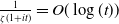 $\frac {1}{\zeta (1+it)} = O(\log (t))$
, see for instance [Reference Montgomery and Vaughan28, Theorem 6.7]. Since the modulus
 $m$
of
 $\chi _D$
satisfies
 $m=O(D)$
, we also have for
 $s$
with
 $\mathrm{Re}(s)=\frac {1}{2}$
:
 \begin{equation*} \frac {1}{\prod _{p\mid m} (1-p^{-2s})} \ll _\epsilon D^\epsilon \end{equation*}
This shows that along the line
 $\operatorname {Re}(s) = \tfrac {1}{2}$
, we have
 \begin{equation} \frac {1}{\zeta (2s) \prod _{p\mid m} (1-p^{-2s})} \ll _\epsilon D^\epsilon \vert t\vert ^{\epsilon }, \end{equation}
with the convention that the left-hand side is interpreted as zero when
 $s = \tfrac {1}{2}$
. Combining the three bounds (83), (84), and (85), we obtain for
 $\mathrm{Re}(s)=\frac {1}{2}$
:
 \begin{equation} \vert F(s;\,\gamma ) \vert \ll _{\epsilon , \Gamma } \mathcal{Q}(\gamma )^{\frac {1}{2}+\epsilon } \mathcal{D}(\gamma )^{\epsilon } (1+\vert t\vert )^\epsilon . \end{equation}
Hence, shifting the line of integration on the right of (78) to
 $\mathrm{Re}(s) = \frac {1}{2}$
and then using (86), we find
 \begin{equation} \sum _{\text{ $q$ sqf }} \mathrm{tr}(\nu _q(\gamma )) \psi ( \frac {q}{x} ) = \frac {1}{2\pi i} \int _{(\frac {1}{2})} F(s;\,\gamma ) x^s \widehat {\psi }(s) ds \ll _{\epsilon ,\psi ,\Gamma } x^{\frac {1}{2}} \mathcal{Q}(\gamma )^{\frac {1}{2}+\epsilon } \mathcal{D}(\gamma )^{\epsilon }. \end{equation}
This completes the proof of the estimate (70) conditional on the Lindelöf hypothesis for quadratic L-functions.
Now, we prove the estimate in (71). Fix a hyperbolic element
 $\gamma \in \Gamma$
with
 \begin{equation} \Vert \gamma \Vert \lt \frac {x^2}{12}. \end{equation}
Recall that the notation
 $p\sim x$
means
 $p\in (\frac {x}{2}, x]$
. It is easy to verify that the condition (88) implies that
 $\gamma \not \equiv \pm I \mod p$
for all
 $p\sim x$
. Assume not. Then, we have
 $\gamma \equiv \pm I \mod p$
for some
 $p\gt \frac {x}{2}$
, which by Lemma 4.8 implies that
 \begin{equation*} \Vert \gamma \Vert \geqslant \frac {p^2}{3} \gt \frac {x^2}{12}, \end{equation*}
contradicting (88). We can now apply Lemma 4.6. We deduce that for all
 $x$
sufficiently large we have
 \begin{equation} p\sim x \Longrightarrow \mathrm{tr}(\nu _p(\gamma )) = \chi _{\mathcal{D}(\gamma )}(p). \end{equation}
Recall once again that if
 $D\in \mathbb{N}$
be a non-square such that
 $D \equiv 0,1 \mod 4$
, then
 $q\mapsto \chi _D(q)$
is a non-principal Dirichlet character of conductor at most
 $4D$
. We now invoke a classical result from the book of Iwaniec-Kowalski [Reference Iwaniec and Kowalski18, Theorem 5.15]: conditional on the GRH for
 $L(s,\chi _D)$
it holds that
 \begin{equation*} \sum _{q\leqslant x} \chi _D(q) \Lambda (q) \ll _\epsilon x^{1/2+\epsilon } D^\epsilon , \end{equation*}
where
 $\Lambda (q)$
is the von Mangoldt function. We can restrict this sum to primes at the cost of an error term of
 $O(x^{1/2+\epsilon })$
, so the above implies that
 \begin{equation} \sum _{\substack {p\leqslant x \\ \text{$p$ prime}}} \chi _D(p) \log (p) \ll _\epsilon x^{1/2+\epsilon } D^\epsilon . \end{equation}
It follows from (89) and (90) applied with
 $D=\mathcal{D}(\gamma )$
that
 \begin{align*} \sum _{\substack {p\sim x \\ \text{$p$ prime}}} \log (p) \mathrm{tr}(\nu _p(\gamma )) &= \sum _{\substack {p\sim x \\ \text{$p$ prime}}} \log (p) \chi _{\mathcal{D}(\gamma )}(p)\\ &= \sum _{\substack {p\leqslant x/2 \\ \text{$p$ prime}}} \log (p) \chi _{\mathcal{D}(\gamma )}(n) - \sum _{\substack {p\leqslant x \\ \text{$p$ prime}}} \log (p) \chi _{\mathcal{D}(\gamma )}(n)\\ &\ll _\epsilon x^{1/2+\epsilon } \mathcal{D}(\gamma )^\epsilon . \end{align*}
Finally, observe that
 $\mathcal{D}(\gamma ) \ll \Vert \gamma \Vert ^2 \ll x^4$
, so the right-hand side of the previous inequality can be further bounded by
 $O_\epsilon (x^{1/2+\epsilon }).$
The proof of Proposition 4.5 is finished.
4.4. Congruence counting estimates
We now establish auxiliary counting bounds for congruence subgroups. Recall the definition of the set
 $Y(\tau )$
in (41). Given a square-free integer
 $q\in \mathbb{N}$
and
 $\tau \gt 0$
we define
 \begin{equation} \mathcal{P}_q (\tau ) \stackrel {\text{def}}{=} \{ (\textbf {a},\textbf {b})\in Y(\tau )\times Y(\tau ) : \text{$\textbf {a}\neq \textbf {b}$ and $\mathcal{Q}(\gamma _{\textbf {a}}^{-1} \gamma _{\textbf {b}}) = q$} \}, \end{equation}
where
 $\mathcal{Q}(\gamma )$
is given in Definition 4.4. The main result of this subsection is
Proposition 4.10 (Bound for
 $\#\mathcal{P}_q (\tau )$
). There exists
 $\tau _0 \gt 0$
such that for all
 $0 \lt \tau \lt \tau _0$
, for all
 $q\in \mathbb{N}$
, and for all
 $\epsilon \gt 0$
, the following inequality holds:
 \begin{equation*} \#\mathcal{P}_q(\tau ) \ll _{\epsilon ,\Gamma } \tau ^{-\epsilon } \left ( \frac {\tau ^{-2}}{q^3} + \frac {\tau ^{-1}}{q} \right ). \end{equation*}
We begin with the following elementary but crucial observation:
Lemma 4.11.
For every hyperbolic element
 $\gamma \in \mathrm{SL}_2(\mathbb{Z})$
, we have
 $\Vert \gamma \Vert \gt \frac {\mathcal{Q}(\gamma )}{\sqrt {3}}$
.
Proof.
Fix a hyperbolic element
 $\gamma \in \mathrm{SL}_2(\mathbb{Z})$
and set
 $q = \mathcal{Q}(\gamma ).$
If
 $q = 1$
, the inequality is trivial, and so we assume that
 $q\geqslant 2.$
Let
 $p_1, \ldots , p_k$
be the distinct prime factors of
 $q$
so that
 $q = p_1 \ldots p_k$
. The condition
 $\mathcal{Q}(\gamma )=q$
implies that for each
 $i=1, \ldots , k$
we have
 $\gamma \equiv \pm I \mod p_i$
and hence also
 $\gamma ^2 \equiv I \mod p_i$
. A simple application of the Chinese Remainder Theorem shows that
 $\gamma ^2 \equiv I \mod q$
. By the submultiplicativity of the Frobenius norm and Lemma 4.8, we then have
 \begin{equation*} \Vert \gamma \Vert ^2 \geqslant \Vert \gamma ^2\Vert \gt \frac {q^2}{3}, \end{equation*}
completing the proof.
As a consequence, we obtain the following helpful estimates:
Lemma 4.12.
For all
 $(\textbf {a},\textbf {b})\in Y(\tau )\times Y(\tau )$
with
 $\textbf {a}\neq \textbf {b}$
we have
-
(i)
$\mathcal{Q}(\gamma _{\textbf {a}}^{-1}\gamma _{\textbf {b}}) \ll _\Gamma \tau ^{-1}$
and
-
(ii)
$\mathcal{D}(\gamma _{\textbf {a}}^{-1}\gamma _{\textbf {b}}) \ll _\Gamma \tau ^{-2}.$


Proof.
Fix a pair of words
 $(\textbf {a},\textbf {b})\in Y(\tau )\times Y(\tau )$
with
 $\textbf {a}\neq \textbf {b}$
. Then
 $\gamma _{\textbf {a}}^{-1} \gamma _{\textbf {b}}\neq I$
because
 $\Gamma$
is freely generated by the elements
 $\{ \gamma _a\}_{a\in \mathcal{A}}$
. It follows that
 $\gamma _{\textbf {a}}^{-1} \gamma _{\textbf {b}}$
is a hyperbolic element, since
 $\Gamma \setminus \{I\}$
consists only of hyperbolic elements. From Lemma 4.11, the submultiplicativity of the Frobenius norm, and Lemma 2.7, we now deduce that
 \begin{equation*} \mathcal{Q}(\gamma _{\textbf {a}}^{-1}\gamma _{\textbf {b}})\ll \Vert \gamma _{\textbf {a}}^{-1}\gamma _{\textbf {b}}\Vert \leqslant \Vert \gamma _{\textbf {a}} \Vert \Vert \gamma _{\textbf {b}}\Vert \ll _\Gamma \tau ^{-1}, \end{equation*}
as claimed. Similarly, we can estimate
 \begin{equation*} \mathcal{D}(\gamma _{\textbf {a}}^{-1}\gamma _{\textbf {b}}) = \mathrm{tr}(\gamma _{\textbf {a}}^{-1}\gamma _{\textbf {b}})^2 - 4\ll \Vert \gamma _{\textbf {a}}^{-1}\gamma _{\textbf {b}}\Vert ^2 \leqslant \Vert \gamma _{\textbf {a}} \Vert ^2 \Vert \gamma _{\textbf {b}}\Vert ^2 \ll _\Gamma \tau ^{-2}, \end{equation*}
completing the proof.
The crucial step towards the proof of Proposition 4.10 is to estimate the cardinality of the set
 \begin{equation} \mathcal{C}_q(x) \stackrel {\text{def}}{=} \{ \gamma \in \mathrm{SL}_2(\mathbb{Z}) : \text{$\mathcal{Q}(\gamma ) = q$ and $\Vert \gamma \Vert \leqslant x$} \}. \end{equation}
Lemma 4.13 (Congruence counting in
 $\mathrm{SL}_2({\mathbb{Z}})$
). For any
 $x\gt 0$
, any square-free integer
 $q\gt 0$
, and any
 $\epsilon \gt 0$
, we have
 \begin{equation*} \# \mathcal{C}_q(x) \ll _\epsilon x^{\epsilon } \left ( \frac {x^2}{q^3}+\frac {x}{q}+1\right ). \end{equation*}
Proof.
For
 $q=1$
the lemma follows from the well-known estimate
 \begin{equation*} \# \{ \gamma \in \mathrm{SL}_2(\mathbb{Z}) : \Vert \gamma \Vert \leqslant x \} \ll x^2 +1. \end{equation*}
We may therefore assume for the rest of the proof that
 $q$
is a square-free integer greater or equal than two. Let
 $q=p_1 \cdots p_k$
be its prime factorization. If
 $\gamma \in \mathrm{SL}_2({\mathbb{Z}})$
is such that
 $\mathcal{Q}(\gamma )=q$
, then for all
 $i=1, \ldots , k$
there exists
 $\xi _i \in \{-1,+1 \}$
such that
 $\gamma \equiv \xi _i I \mod p_i$
. Hence, for every
 $k$
-tuple of signs
 $\xi = (\xi _1, \ldots , \xi _k) \in \{-1,+1 \}^k$
we define the set
 \begin{equation*} \mathcal{S}(x,\xi ) \stackrel {\text{def}}{=} \{ \gamma \in \mathrm{SL}_2(\mathbb{Z}) : \text{$\gamma \equiv \xi _i I \mod p_i$ for all $i=1, \ldots , k$ and $\Vert \gamma \Vert \leqslant x$} \} \end{equation*}
so that
 \begin{equation*} \mathcal{C}_q(x) = \bigsqcup _{\xi \in \{-1,+1 \}^k}\mathcal{S}(x,\xi ). \end{equation*}
We claim that for each
 $\xi \in \{-1,+1 \}^k$
we have
 \begin{equation} \# \mathcal{S}(x,\xi ) \ll _\epsilon x^{\epsilon } \left ( \frac {x^2}{q^3}+\frac {x}{q}+1\right ), \end{equation}
where the implied constant is uniform in
 $\xi$
. Before proving this estimate let us demonstrate how to derive Lemma 4.13 from it. From (93) it follows that
 \begin{equation*} \#\mathcal{C}_q(x) = \sum _{\xi \in \{-1,+1 \}^k}\# \mathcal{S}(x,\xi ) \ll _\epsilon 2^k x^{\epsilon } \left ( \frac {x^2}{q^3}+\frac {x}{q}+1\right ). \end{equation*}
It remains to estimate the factor
 $2^k$
on the right. Observe that
 $k=o(\log q)$
and that the set
 $\mathcal{C}_q(x)$
is empty unless
 $q = O(x)$
. Thus, we may assume that
 $q = O(x)$
, in which case
 $2^k = O_\epsilon (q^\epsilon ) = O_\epsilon (x^\epsilon )$
for any
 $\epsilon \gt 0$
. Inserting this into the previous bound proves the lemma.
It remains to prove (93). Fix
 $\xi = (\xi _1, \ldots , \xi _k) \in \{-1,+1 \}^k$
and note that each element
 \begin{equation} \gamma \stackrel {\text{def}}{=} \begin{pmatrix} a&b\\c&d\end{pmatrix} \in \mathcal{S}(x,\xi ), \end{equation}
satisfies the congruence relations
 \begin{equation} a \equiv d \equiv \xi _i \mod p_i, \quad b \equiv c \equiv 0 \mod p_i, \quad i=1,\ldots , k \end{equation}
Moreover, by Lemma 4.8, the trace
 $\textrm {tr}(\gamma ) = a+d$
satisfies
 \begin{equation*} a+d \equiv 2\xi _i \mod p_i^2, \quad i=1,\ldots , k. \end{equation*}
Recall that
 $p_1, \ldots , p_k$
are distinct primes and that
 $q=p_1 \cdots p_k$
. Applying the Chinese Remainder Theorem to the simultaneous congruences (94), respectively (95), we see that there are integers
 $r(\xi )$
and
 $t(\xi )$
, depending only on the chosen
 $\xi$
, such that
 \begin{equation*} a \equiv d \equiv r(\xi ) \mod q \end{equation*}
and
 \begin{equation*} a+d \equiv t(\xi ) \mod q^2. \end{equation*}
Observe also that
 $\Vert \gamma \Vert \leqslant 2\max \{ \vert a\vert , \vert b\vert , \vert c\vert , \vert d\vert \}$
. Hence, estimating the cardinality of
 $\mathcal{S}(x,\xi )$
amounts to estimating the number of quadruples
 $ (a,b,c,d)\in {\mathbb{Z}}^4$
satisfying the properties
-
•
$ad-bc = 1,$
-
•
$\max \{ \vert a\vert , \vert b\vert , \vert c\vert , \vert d\vert \} \leqslant 2x$
, -
•
$a,d\equiv r(\xi ) \mod q$
and
$b,c\equiv 0 \mod q$
, and -
•
$a+d\equiv t(\xi ) \mod q^2.$


The argument is now very similar to the one given in [Reference Calderón and Magee7, Lemma 18]. The number of these quadruples with
 $bc= 0$
is at most
 $O(x/q +1)$
. From now on, we assume that
 $bc\neq 0$
. The conditions
 $\vert a\vert \leqslant x$
and
 $a\equiv r(\xi ) \mod q$
imply that there are at most
 $4x/q + 1$
choices for
 $a$
. The condition
 $d \equiv t(\xi )-a \mod q^2$
implies that there at most
 $4x/q^2 + 1$
choices for
 $d$
. Now, assume
 $(a,d)$
has already been chosen. Then, there are at most
 $D(ad + 1)$
choices for
 $(b,c)\in {\mathbb{Z}}^2$
, where
 $D(n)$
denotes the number of
 $(b,c)\in {\mathbb{Z}}^2$
satisfying
 $bc = n$
. The well-known bound for the divisor function gives us
 $D(n)\ll _\epsilon \vert n\vert ^\epsilon$
for all
 $n\neq 0$
. Hence, since
 $0\neq bc = ad - 1$
and
 $ad-1\ll x^2$
, we deduce that there are at most
 $O_\epsilon (x^\epsilon )$
choices for
 $(b,c)\in {\mathbb{Z}}^2$
satisfying the above conditions. We end up with at most
 \begin{equation*} x^\epsilon \left ( \frac {x}{q^2} + 1 \right ) \left ( \frac {x}{q} + 1 \right ) \ll x^{\epsilon } \left ( \frac {x^2}{q^3}+\frac {x}{q}+1\right ) \end{equation*}
choices for quadruples with the above properties, as claimed.
We can now give the
Proof of Proposition 4.10. Recall that we aim to prove the estimate
 \begin{equation*} \mathcal{P}_q (\tau ) \stackrel {\text{def}}{=} \{ (\textbf {a},\textbf {b})\in Y(\tau )\times Y(\tau ) : \text{$\textbf {a}\neq \textbf {b}$ and $\mathcal{Q}(\gamma _{\textbf {a}}^{-1} \gamma _{\textbf {b}}) = q$} \} \ll _{\epsilon ,\Gamma } \tau ^{-\epsilon } \left ( \frac {\tau ^{-2}}{q^3} + \frac {\tau ^{-1}}{q} \right ). \end{equation*}
We will closely follow the strategy used in the paper of Calderón-Magee [Reference Calderón and Magee7] to estimate a similar set but we utilize slightly different notations.
By Lemma 4.12, we have
 $\mathcal{Q}(\gamma _{\textbf {a}}^{-1}\gamma _{\textbf {b}}) \ll _\Gamma \tau ^{-1}$
for all
 $(\textbf {a},\textbf {b})\in Y(\tau )\times Y(\tau )$
with
 $\textbf {a} \neq \textbf {b},$
and so we may assume throughout that
 $q \ll _\Gamma \tau ^{-1}$
. All the implied constants are allowed to depend on
 $\Gamma$
, so we drop
 $\Gamma$
from the notation, writing only
 $\asymp$
and
 $\ll$
instead of
 $\asymp _\Gamma$
and
 $\ll _\Gamma$
.
Observe that for any
 $(\textbf {a},\textbf {b}) \in \mathcal{P}_q (\tau )$
, there is a unique decomposition
 \begin{equation} \textbf {a} = \textbf {c} \textbf {a}_0 \textbf {d}, \quad \textbf {b} = \textbf {c} \textbf {b}_0 \textbf {d} \end{equation}
with
 $\textbf {a}_0\textbf {b}_0,\textbf {c},\textbf {d}\in \mathcal{W}$
satisfying
 $\textbf {c} \to \textbf {a}_0, \textbf {b}_0 \to \textbf {d}$
and
 $\overline {\textbf {a}}_0 \to \textbf {b}_0$
. By Lemma 2.5, we have
 \begin{equation} \Upsilon _{\textbf {c}}\Upsilon _{\textbf {a}_0}\Upsilon _{\textbf {d}} \asymp \Upsilon _{\textbf {a}} \asymp \tau , \quad \Upsilon _{\textbf {c}}\Upsilon _{\textbf {b}_0}\Upsilon _{\textbf {d}} \asymp \Upsilon _{\textbf {b}} \asymp \tau . \end{equation}
as well as
 \begin{equation} \Upsilon _{\overline {\textbf {a}}_0 \textbf {b}_0} \asymp \Upsilon _{\textbf {a}_0} \Upsilon _{\textbf {b}_0}. \end{equation}
Given
 $c,d\in \mathbb{N}$
, we define
 \begin{equation*} \mathcal{P}_q (\tau , c,d) \stackrel {\text{def}}{=} \# \{ (\textbf {a},\textbf {b})\in \mathcal{P}_q (\tau ) : 2^{-(c+1)} \leqslant \Upsilon _{\textbf {c}} \leqslant 2^{-c}, 2^{-(d+1)} \leqslant \Upsilon _{\textbf {d}} \leqslant 2^{-d} \}. \end{equation*}
as well as
 \begin{equation*} \mathcal{S}_q (\tau , c,d) \stackrel {\text{def}}{=} \sum _{ (\textbf {a},\textbf {b}) \in \mathcal{P}_q (\tau , c,d) } \Upsilon _{\textbf {c}}^{\delta } \Upsilon _{\overline {\textbf {a}_0} \textbf {b}_0}^{\delta /2} \Upsilon _{\textbf {d}}^{\delta }. \end{equation*}
By (97) and (98),
 $\Upsilon _{\textbf {c}}^{\delta } \Upsilon _{\overline {\textbf {a}_0} \textbf {b}_0}^{\delta /2} \Upsilon _{\textbf {d}}^{\delta } \asymp \tau ^\delta ,$
whence
 \begin{equation*} \mathcal{S}_q (\tau , c,d) \asymp \tau ^\delta \mathcal{P}_q (\tau , c,d). \end{equation*}
Now, we let
 $\mathcal{E}_q(\tau ,c,d)$
, respectively,
 $ \mathcal{M}_q(\tau ,c,d)$
be the sets consisting of all words
 $\textbf {c},\textbf {d}$
, respectively,
 $\overline {\textbf {a}_0} \textbf {b}_0$
for which we have decompositions
 $\textbf {a} = \textbf {c} \textbf {a}_0 \textbf {d}$
and
 $ \textbf {b} = \textbf {c} \textbf {b}_0 \textbf {d}$
as in (96) with
 $(\textbf {a},\textbf {b})\in \mathcal{P}_q(\tau , c,d).$
Recall that the word lengths
 $\vert \textbf {a}_0\vert , \vert \textbf {b}_0\vert , \vert \textbf {c}\vert , \vert \textbf {d}\vert$
are of size
 $O(\log (\tau ^{-1}))$
by Lemma 2.7. In particular, the word length of
 $\overline {\textbf {a}}_0 \textbf {b}_0$
is at most
 $O(\log (\tau ^{-1}))$
. Thus, the map
 \begin{equation*} \mathcal{P}_q(\tau ,c,d) \to \mathcal{E}_q(\tau ,c,d) \times \mathcal{E}_q(\tau ,c,d) \times \mathcal{M}_q(\tau ,c,d), \quad (\textbf {a},\textbf {b})\mapsto (\textbf {c},\textbf {d}, \overline {\textbf {a}}_0 \textbf {b}_0) \end{equation*}
is at most
 $m$
-to-
 $1$
for some
 $m = O(\log (\tau ^{-1}))$
. It follows that
 \begin{align*} \mathcal{S}_q (\tau , c,d) &\ll \log (\tau ^{-1} ) \sum _{ \textbf {c} \in \mathcal{E}_q (\tau , c,d) } \sum _{ \textbf {f} \in \mathcal{M}_q (\tau , c,d) } \sum _{ \textbf {d}\in \mathcal{E}_q (\tau , c,d) } \Upsilon _{\textbf {c}}^{\delta } \Upsilon _{\textbf {f}}^{\delta /2} \Upsilon _{\textbf {d}}^{\delta }\\ & \ll \log (\tau ^{-1} ) \left ( \sum _{ \textbf {c} \in \mathcal{E}_q (\tau , c,d) } \Upsilon _{\textbf {c}}^{\delta }\right )^2 \sum _{ \textbf {f} \in \mathcal{M}_q (\tau , c,d) } \Upsilon _{\textbf {f}}^{\delta /2}. \end{align*}
Using the same word count as above, we deduce that
 $\mathcal{E}_q (\tau , c,d)$
is contained within
 $\mathcal{W}_{\leqslant N} = \bigcup _{n=1}^N \mathcal{W}_n$
for some
 $N=O(\log (\tau ^{-1}))$
. It is known from Naud [Reference Naud29, Lemma 3.1] that for any
 $n\in \mathbb{N},$
 \begin{equation*} \sum _{\textbf {c}\in \mathcal{W}_n} \Upsilon _{\textbf {c}}^\delta \ll 1. \end{equation*}
Therefore,
 \begin{equation*} \sum _{ \textbf {c} \in \mathcal{E}_q (\tau , c,d) } \Upsilon _{\textbf {c}}^{\delta } \ll \sum _{n=1}^N \sum _{\textbf {c}\in \mathcal{W}_n} \Upsilon _{\textbf {c}}^\delta \ll N \ll \log (\tau ^{-1}). \end{equation*}
Hence,
 \begin{equation} \mathcal{S}_q (\tau , c,d) \ll \log (\tau ^{-1} )^3 \sum _{ \textbf {f} \in \mathcal{M}_q (\tau , c,d) } \Upsilon _{\textbf {f}}^{\delta /2} \end{equation}
Next, we denote by
 $M_q(\tau , c,d )$
the maximum of
 $\Upsilon _{\textbf {f}}$
among all
 $\textbf {f}\in \mathcal{M}_q(\tau , c,d )$
. From (97) and (98), it follows that for all
 $(\textbf {a},\textbf {b})\in \mathcal{P}_q(\tau ,c,d)$
,
 \begin{equation*} \Upsilon _{\overline {\textbf {a}}_0 \textbf {b}_0} \asymp \Upsilon _{\textbf {a}_0} \Upsilon _{\textbf {b}_0} \asymp \left ( \frac {\tau }{\Upsilon _{\textbf {c}}\Upsilon _{\textbf {d}}}\right )^2, \end{equation*}
from which we deduce
 \begin{equation} M_q(\tau , c,d ) \ll 2^{2(c+d)} \tau ^2. \end{equation}
Inserting this into (99), we get
 \begin{align*} \mathcal{S}_q (\tau , c,d) &\ll \log (\tau ^{-1} )^3 M_q(\tau , c,d )^{\delta /2} \#\mathcal{M}_q(\tau ,c,d) \\ &\ll \log (\tau ^{-1} )^3 2^{\delta (c+d)} \tau ^{\delta } \#\mathcal{M}_q(\tau ,c,d). \end{align*}
By (100) and Lemma 2.7, each
 $\textbf {f} \in \mathcal{M}_q(\tau ,c,d)$
satisfies
 \begin{equation} \Vert \gamma _{\textbf {f}}\Vert \leqslant c 2^{-(c+d)} \tau ^{-1} \end{equation}
for some
 $c=c(\Gamma )\gt 0$
. It follows that
 $\mathcal{M}_q(\tau ,c,d) \subseteq \mathcal{C}_q( c 2^{-(c+d)} \tau ^{-1})$
, where
 $\mathcal{C}_q(\cdot )$
is the set defined in (92). Therefore, applying Lemma 4.13, we obtain
 \begin{align*} \#\mathcal{M}_q(\tau ,c,d) &\ll \# \mathcal{C}( c 2^{-(c+d)} \tau ^{-1},q) \\ &\ll 2^{-(c+d)\epsilon } \tau ^{-\epsilon } \left ( \frac {2^{-2(c+d)} \tau ^{-2}}{q^3} + \frac {2^{-(c+d)} \tau ^{-1}}{q} + 1 \right ). \end{align*}
We can now put everything together. Let
 $\mathcal{I}_q(\tau )$
be the set of all
 $(c,d)\in \mathbb{N}^2$
for which
 $\mathcal{M}_q (\tau ,c,d)$
is non-empty. We can then estimate
 \begin{align*} \#\mathcal{P}_q (\tau ) &= \sum _{(c,d)\in \mathcal{I}_q(\tau )} \# \mathcal{P}_q (\tau ,c,d)\\ &\ll \tau ^{-\delta } \sum _{(c,d)\in \mathcal{I}_q(\tau )} \mathcal{S}_q (\tau ,c,d) \\ &\ll \log (\tau ^{-1} )^3 \sum _{(c,d)\in \mathcal{I}_q(\tau )} 2^{\delta (c+d)} \# \mathcal{M}_q (\tau ,c,d) \\ &\ll _\epsilon \log (\tau ^{-1} )^3 \sum _{(c,d)\in \mathcal{I}_q(\tau )} 2^{(\delta -\epsilon )(c+d)} \tau ^{-\epsilon } \left ( \frac {2^{-2(c+d)} \tau ^{-2}}{q^3} + \frac {2^{-(c+d)} \tau ^{-1}}{q} + 1 \right ). \end{align*}
Since
 $\delta \lt 1$
, we have
 $1 - \delta + \epsilon \gt 0$
for any
 $\epsilon \gt 0$
. Thus, using the summation of a geometric series, we obtain
 \begin{equation*} \sum _{(c,d) \in \mathcal{I}_q(\tau )} 2^{-(1 - \delta + \epsilon )(c + d)} \leqslant \sum _{(c,d) \in \mathbb{N}^2} 2^{-(1 - \delta + \epsilon )(c + d)} = \left (\sum _{c\in \mathbb{N}} 2^{-(1 - \delta + \epsilon )c}\right )^2 \ll 1. \end{equation*}
Similarly, we have
 \begin{equation*} \sum _{(c,d) \in \mathcal{I}_q(\tau )} 2^{-(2 - \delta + \epsilon )(c + d)} \ll 1. \end{equation*}
In addition, observe also that
 $\log (\tau ^{-1} )\ll _\epsilon \tau ^{-\epsilon }$
. Thus, we arrive at
 \begin{equation} \#\mathcal{P}_q (\tau ) \ll _\epsilon \tau ^{-\epsilon } \left ( \frac {\tau ^{-2}}{q^3} + \frac {\tau ^{-1}}{q} + \sum _{(c,d)\in \mathcal{I}_q(\tau )} 2^{(\delta -\epsilon )(c+d)} \right ). \end{equation}
To estimate the remaining sum note that (101) and Lemma 4.11 imply that
 $\mathcal{M}_q(\tau , c,d)$
is non-empty only when
 $q \ll 2^{-(c+d)}\tau ^{-1}$
, which is to say that
 \begin{equation*} \mathcal{I}_q(\tau )\subseteq \left \{ (c,d)\in \mathbb{N}^2 : 2^{c+d} \leqslant C \frac {\tau ^{-1}}{q} \right \} \end{equation*}
for some constant
 $C=C(\Gamma )\gt 0$
. Recalling that we always have
 $q \ll \tau ^{-1}$
, we can estimate
 \begin{equation*} \sum _{(c,d)\in \mathcal{I}_q(\tau )} 2^{(\delta -\epsilon )(c+d)} \ll \sum _{1\leqslant n \leqslant \log _2( \frac {\tau ^{-1}}{q} )+C'} n 2^{(\delta -\epsilon )n} \ll \log _2\left( \frac {\tau ^{-1}}{q} \right) \left ( \frac {\tau ^{-1}}{q} \right )^{\delta -\epsilon }. \end{equation*}
Plugging this into (102) we find that
 \begin{equation*} \#\mathcal{P}_q (\tau ) \ll _\epsilon \tau ^{-\epsilon } \left ( \frac {\tau ^{-2}}{q^3} + \frac {\tau ^{-1}}{q} + \log _2\left( \frac {\tau ^{-1}}{q} \right) \left ( \frac {\tau ^{-1}}{q} \right )^{\delta -\epsilon } \right ). \end{equation*}
Clearly, the third term on the right is smaller than the middle term. The proof of Proposition 4.10 is thus complete.
The next lemma is what actually matters to us. It provides an estimate for a special sum, which we will encounter later in the proof of Proposition 4.3:
Lemma 4.14 (Estimate for a special sum). There exists
 $\tau _0 = \tau _0(\Gamma )\gt 0$
such that for all
 $\tau$
in the range
 $0 \lt \tau \lt \tau _0$
and for any
 $\epsilon \gt 0$
, the following estimate holds:
 \begin{equation*} \sum _{\substack { \textbf {a},\textbf {b}\in Y(\tau ) \\ \textbf {a}\neq \textbf {b}}} \mathcal{Q}(\gamma _{\textbf {a}}^{-1}\gamma _{\textbf {b}})^{1/2} \ll _{\epsilon ,\Gamma } \tau ^{-\max \{ \frac {3}{2}\delta + \frac {1}{2}, \frac {3}{2}\}-\epsilon }. \end{equation*}
Proof.
By Lemma 4.12, it holds that for all words
 $\textbf {a},\textbf {b}\in Y(\tau )$
with
 $\textbf {a}\neq \textbf {b}$
we have
 $\mathcal{Q}(\gamma _{\textbf {a}}^{-1}\gamma _{\textbf {b}}) \leqslant C\tau ^{-1}$
for some
 $C=C(\Gamma )\gt 0$
. Hence, we can estimate
 \begin{equation*} \sum _{\substack { \textbf {a},\textbf {b}\in Y(\tau ) \\ \textbf {a}\neq \textbf {b}}} \mathcal{Q}(\gamma _{\textbf {a}}^{-1}\gamma _{\textbf {b}})^{1/2} \leqslant \sum _{1\leqslant q \leqslant C \tau ^{-1}} q^{1/2} \# \mathcal{P}_q(\tau ), \end{equation*}
where the sum on the right is over square-free integers. Now, we split this sum for some
 $q_0 \in \mathbb{N}$
(to be chosen below) as follows:
 \begin{equation*} \sum _{1\leqslant q \leqslant C \tau ^{-1/2}} q^{1/2} \#\mathcal{P}_q(\tau ) = \sum _{1\leqslant q \leqslant q_0} q^{1/2} \#\mathcal{P}_q(\tau ) + \sum _{q_0 \lt q \leqslant C \tau ^{-1/2}} q^{1/2} \#\mathcal{P}_q(\tau ) \end{equation*}
The sets
 $\mathcal{P}_q (\tau )$
(
 $q\in \mathbb{N}$
) are pairwise disjoint, so we can use Lemma 2.7 to estimate the first sum on the right as follows:
 \begin{equation*} \sum _{1\leqslant q \leqslant q_0} q^{1/2} \#\mathcal{P}_q(\tau ) \leqslant q_0^{1/2} \sum _{1\leqslant q \leqslant q_0} \#\mathcal{P}_q(\tau ) \ll _\epsilon q_0^{1/2} \left ( \sum _{\textbf {a},\textbf {b}\in Y(\tau )} 1\right ) \ll q_0^{1/2} \tau ^{-2\delta }. \end{equation*}
For the second sum, we invoke Proposition 4.10:
 \begin{align*} \sum _{q_0 \lt q \leqslant C \tau ^{-1/2}} q^{1/2} \#\mathcal{P}_q(\tau ) &\ll _{\epsilon ,\Gamma } \tau ^{-\epsilon } \sum _{q_0 \lt q \leqslant C \tau ^{-1}} q^{1/2} \left ( \frac {\tau ^{-2}}{q^{3}} + \frac {\tau ^{-1}}{q} \right )\\ &= \tau ^{-\epsilon } \sum _{q_0 \lt q \leqslant C \tau ^{-1}} \left ( \frac {\tau ^{-2}}{q^{5/2}} + \frac {\tau ^{-1}}{q^{1/2}} \right )\\ &\ll \tau ^{-\epsilon } \left ( \sum _{q \gt q_0}\frac {\tau ^{-2}}{q^{5/2}} + \sum _{1 \leqslant q \leqslant C \tau ^{-1}} \frac {\tau ^{-1}}{q^{1/2}} \right ) \\ &\ll \tau ^{-\epsilon } \left ( \frac {\tau ^{-2}}{q_0^{3/2}} + \tau ^{-3/2} \right ). \end{align*}
Combining the previous two bounds and taking
 $q_0 = \tau ^{-(1-\delta )}$
, yields (up to
 $\tau ^{-\epsilon }$
-factors)
 \begin{equation*} q_0^{1/2} \tau ^{-2\delta } + \frac {\tau ^{-2}}{q_0^{3/2}} + \tau ^{-5/4} \ll \tau ^{-( \frac {3}{2}\delta + \frac {1}{2} )} + \tau ^{-3/2} \ll \tau ^{-\max \{ \frac {3}{2}\delta + \frac {1}{2}, \frac {3}{2}\}}, \end{equation*}
thereby yielding the sought-after estimate.
4.5. Proof of Proposition 4.3
We now combine the ingredients above to prove Proposition 4.3 from which Proposition 4.2 and thus the main results of this paper follow.
Proof of Proposition
4.3
. Let
 $\sigma_0 \gt 0$
and
 $s=\sigma + it$
with
 $\sigma \geqslant \sigma_0.$
Recall that our goal is to prove the following conditional estimates:
-
(i) Assume the Lindelöf Hypothesis for quadratic L-functions. Assume that
$\delta \gt \frac {1}{2}$
. For all
$x\gg _\Gamma 1$
, we have with
$A = \max \left \{ \frac {1+\delta }{3}, 1-\frac {2}{3}\delta \right \}$
and
$\tau = x^{-1/A}$
,
\begin{equation*} \sum _{\substack { q\sim x \\ \text{ $q$ sqf } }} \Vert \mathcal{L}_{\tau , s, \nu _q} \Vert _{\mathrm{HS}}^2 \ll _{\epsilon ,\Gamma } C^{\sigma_0 } e^{C \vert t\vert } x^{1 - \frac {2}{A} ( \sigma_0 - \frac {\delta + A}{2} ) + \epsilon }. \end{equation*}
-
(ii) Assume the GRH for quadratic
$L$
-functions. Assume that
$\delta \gt \frac {3}{4}$
. For all
$x\gg _\Gamma 1$
, we have with
$A = \frac {2\delta }{3}$
and
$\tau = x^{-1/A}$
,
\begin{equation*} \sum _{\substack { p\sim x \\ \text{$p$ prime} }} \Vert \mathcal{L}_{\tau , s,\nu _p} \Vert _{\mathrm{HS}}^2 \ll _{\epsilon ,\Gamma } C^{\sigma_0 } e^{C \vert t\vert } x^{1 - \frac {2}{A} ( \sigma_0 - \frac {\delta + A}{2} ) + \epsilon }. \end{equation*}


Throughout,
 $C \gt 0$
is a constant depending only on
 $\Gamma$
whose precise value changes from line to line. By Lemma 2.8, the Hilbert–Schmidt norm of
 $\mathcal{L}_{\tau ,s,\rho }$
can be expressed for any finite-dimensional unitary representation
 $\rho \colon \Gamma \to \mathrm{U}(V)$
as
 \begin{equation} \Vert \mathcal{L}_{\tau ,s,\rho } \Vert _{\mathrm{HS}}^2 = \sum _{b\in \mathcal{A}}\sum _{\substack { \textbf {a},\textbf {b}\in Y(\tau ) \\ \textbf {a},\textbf {b}\to b }} \mathrm{tr}\left (\rho ( \gamma _{\textbf {a}}^{-1} \gamma _{\textbf {b}} )\right ) \mathcal{I}_{\textbf {a},\textbf {b}}^{(b)}, \end{equation}
where
 $\mathcal{I}_{\textbf {a},\textbf {b}}^{(b)}$
is independent of
 $\rho$
and satisfies the following bound:
 \begin{equation} \vert \mathcal{I}_{\textbf {a},\textbf {b}}^{(b)}\vert \ll (C \tau )^{2\sigma_0 } e^{C \vert t\vert }. \end{equation}
To prove the bound in (i), fix a smooth bump function
 $\psi \colon (0,\infty )\to {\mathbb{R}}$
satisfying
 $\psi \equiv 1$
on
 $[\frac {1}{2},1]$
and
 $\textrm {supp}(\psi ) = [\frac {1}{4},\frac {5}{4}]$
. Using (103), we then have
 \begin{align} \sum _{\substack { q \sim x \\ \text{ $q$ sqf }}} \Vert \mathcal{L}_{\tau ,s,\nu _q} \Vert _{\mathrm{HS}}^2 &\leqslant \sum _{\text{ $q$ sqf }} \psi ( \frac {q}{x} ) \Vert \mathcal{L}_{\tau ,s,\nu _q} \Vert _{\mathrm{HS}}^2 \end{align}
 \begin{align} &= \sum _{b\in \mathcal{A}}\sum _{\substack { \textbf {a},\textbf {b}\in Y(\tau ) \\ \textbf {a},\textbf {b}\to b }} \left ( \sum _{\text{ $q$ sqf }} \psi ( \frac {q}{x} ) \mathrm{tr}\left (\nu _q( \gamma _{\textbf {a}}^{-1} \gamma _{\textbf {b}} )\right )\right ) \mathcal{I}_{\textbf {a},\textbf {b}}^{(b)}. \end{align}
Let us focus on the non-diagonal terms
 $(\textbf {a},\textbf {b})\in Y(\tau )\times Y(\tau )$
with
 $\textbf {a}\neq \textbf {b}$
. Recall that
 $\textbf {a}\neq \textbf {b}$
implies that
 $ \gamma _{\textbf {a}}^{-1} \gamma _{\textbf {b}}$
is hyperbolic. In this case, Proposition 4.5 tells us that under the Lindelöf Hypothesis for quadratic L-functions, we have
 \begin{equation*} \sum _{\text{ $q$ sqf }} \psi ( \frac {q}{x} ) \mathrm{tr}\left (\nu _q( \gamma _{\textbf {a}}^{-1} \gamma _{\textbf {b}} )\right ) \ll _{\epsilon } x^{\frac {1}{2}} \mathcal{Q}(\gamma _{\textbf {a}}^{-1}\gamma _{\textbf {b}})^{\frac {1}{2}+\epsilon } \mathcal{D}(\gamma _{\textbf {a}}^{-1}\gamma _{\textbf {b}})^{\epsilon }. \end{equation*}
Using Lemma 4.12, we can estimate
 $\mathcal{Q}( \gamma _{\textbf {a}}^{-1}\gamma _{\textbf {b}} ) \ll \tau ^{-1}$
and
 $\mathcal{D}(\gamma _{\textbf {a}}^{-1}\gamma _{\textbf {b}} ) \ll \tau ^{-2}.$
Therefore, if we assume that
 $\tau ^{-1} \asymp x^{1/A}$
for some absolute constant
 $A\gt 0$
(which we will specify below), we obtain the somewhat simpler bound
 \begin{equation} \sum _{\text{ $q$ sqf }} \psi ( \frac {q}{x} ) \mathrm{tr}\left (\nu _q( \gamma _{\textbf {a}}^{-1} \gamma _{\textbf {b}} )\right )\ll _\epsilon \tau ^{-\epsilon } x^{1/2} \mathcal{Q}(\gamma _{\textbf {a}}^{-1}\gamma _{\textbf {b}})^{1/2}. \end{equation}
Meanwhile, by Lemma 4.9 we have
 \begin{equation} \mathrm{tr}(\nu _q( I )) = \dim (\nu _q) \ll _\Gamma q. \end{equation}
Inserting the bounds (104), (107), and (108) into (106), and then using Lemma 2.7 to estimate the cardinality of the set
 $ Y(\tau )$
, we obtain
 \begin{align*} \sum _{\substack { q \sim x \\ \text{ $q$ sqf }}} \Vert \mathcal{L}_{\tau ,s,\nu _q} \Vert _{\mathrm{HS}}^2 &\ll \sum _{b\in \mathcal{A}}\sum _{\substack { \textbf {a}\in Y(\tau ) \\ \textbf {a}\to b }} \left ( \sum _{\text{ $q$ sqf }} \psi ( \frac {q}{x} ) q\right ) \mathcal{I}_{\textbf {a},\textbf {a}}^{(b)} + \sum _{b\in \mathcal{A}}\sum _{\substack { \textbf {a},\textbf {b}\in Y(\tau ) \\ \textbf {a},\textbf {b}\to b \\ \textbf {a}\neq \textbf {b} }} \left \vert \sum _{\text{ $q$ sqf }} \psi ( \frac {q}{x} ) \mathrm{tr}\left (\nu _q( \gamma _{\textbf {a}}^{-1} \gamma _{\textbf {b}} )\right )\right \vert \mathcal{I}_{\textbf {a},\textbf {b}}^{(b)}\\ &\ll _\epsilon (C \tau )^{2\sigma_0 } e^{C \vert t\vert } \left ( x^2 \vert Y(\tau )\vert + \tau ^{-\epsilon } x^{1/2} \sum _{b\in \mathcal{A}}\sum _{\substack { \textbf {a},\textbf {b}\in Y(\tau ) \\ \textbf {a},\textbf {b}\to b \\ \textbf {a}\neq \textbf {b} }} \mathcal{Q}( \gamma _{\textbf {a}}^{-1}\gamma _{\textbf {b}} )^{1/2}\right ) \\ &\ll _\epsilon (C \tau )^{2\sigma_0 } e^{C \vert t\vert } \left ( x^2 \tau ^{-\delta } + \tau ^{-\epsilon } x^{1/2} \sum _{\substack { \textbf {a},\textbf {b}\in Y(\tau ) \\ \textbf {a}\neq \textbf {b} }} \mathcal{Q}( \gamma _{\textbf {a}}^{-1}\gamma _{\textbf {b}} )^{1/2} \right ). \end{align*}
The remaining sum in the previous line can be estimated using Lemma 4.14. We obtain
 \begin{equation*} \sum _{\substack { q \sim x \\ \text{ $q$ sqf }}} \Vert \mathcal{L}_{\tau ,s,\nu _q} \Vert _{\mathrm{HS}}^2 \ll _\epsilon (C \tau )^{2\sigma } e^{C \vert t\vert } \left ( x^2 \tau ^{-\delta } + x^{\frac {1}{2}+\epsilon } \tau ^{-\max \{ \frac {3}{2}\delta + \frac {1}{2}, \frac {3}{2}\}-\epsilon } \right ). \end{equation*}
It remains to choose
 $\tau$
optimally. This may be done by taking
 $\tau = x^{-1/A}$
with
 $A=\max \left \{ \frac {1+\delta }{3}, 1-\frac {2}{3}\delta \right \}$
to balance both terms on the right. This leads to the final upper bound
 \begin{equation*} \sum _{\substack { q \sim x \\ \text{ $q$ sqf }}} \Vert \mathcal{L}_{\tau ,s,\nu _q} \Vert _{\mathrm{HS}}^2 \ll _\epsilon C^{2\sigma_0 } e^{C \vert t\vert } x^{1 - \frac {2}{A} ( \sigma_0 - \frac {\delta + A}{2} ) + \epsilon }. \end{equation*}
This settles the estimate in (i).
We now turn to the proof of the estimate in (ii). Similarly as before, we expand the Hilbert–Schmidt norm of
 $ \mathcal{L}_{\tau ,s,\nu _p}$
using the identity in (103). Applying the prime number theorem and the same estimates from above, we find
 \begin{align} \sum _{\substack { p \sim x \\ \text{$p$ prime}}} \Vert \mathcal{L}_{\tau ,s,\nu _p} \Vert _{\mathrm{HS}}^2 &\leqslant \sum _{\substack { p \sim x \\ \text{$p$ prime}}} \log (p) \Vert \mathcal{L}_{\tau ,s,\nu _p} \Vert _{\mathrm{HS}}^2 \end{align}
 \begin{align} &\leqslant \sum _{b\in \mathcal{A}}\sum _{\substack { \textbf {a}\in Y(\tau ) \\ \textbf {a}\to b }} \left ( \sum _{\substack { p \sim x \\ \text{$p$ prime}}} \log (p) p\right ) \mathcal{I}_{\textbf {a},\textbf {a}}^{(b)} + \sum _{b\in \mathcal{A}}\sum _{\substack { \textbf {a},\textbf {b}\in Y(\tau ) \\ \textbf {a},\textbf {b}\to b \\ \textbf {a}\neq \textbf {b} }} \left \vert \sum _{\substack { p \sim x \\ \text{$p$ prime}}} \log (p)\mathrm{tr}\left (\nu _p( \gamma _{\textbf {a}}^{-1} \gamma _{\textbf {b}} )\right )\right \vert \mathcal{I}_{\textbf {a},\textbf {b}}^{(b)} \nonumber \\ &\ll (C \tau )^{2\sigma_0 } e^{C \vert t\vert } \left ( x^2 \tau ^{-\delta } + \sum _{b\in \mathcal{A}}\sum _{\substack { \textbf {a},\textbf {b}\in Y(\tau ) \\ \textbf {a},\textbf {b}\to b \\ \textbf {a}\neq \textbf {b} }} \left \vert \sum _{\substack { p \sim x \\ \text{$p$ prime}}} \log (p)\mathrm{tr}\left (\nu _p( \gamma _{\textbf {a}}^{-1} \gamma _{\textbf {b}} )\right )\right \vert \right ). \end{align}
To estimate the non-diagonal sum in the last line, we appeal to the second estimate in Proposition 4.5. Fix words
 $\textbf {a},\textbf {b}\in Y(\tau )$
with
 $\textbf {a}\neq \textbf {b}$
. Lemma 2.7 and the submultiplicativity of the Frobenius norm imply that
 \begin{equation*} \Vert \gamma _{\textbf {a}}^{-1} \gamma _{\textbf {b}} \Vert \leqslant \Vert \gamma _{\textbf {a}} \Vert \Vert \gamma _{\textbf {b}} \Vert \lt C\tau ^{-1}. \end{equation*}
for some
 $C=C(\Gamma )\gt 0$
. Assume from now on that
 $\tau \gt 12 C x^{-2}$
so that
 \begin{equation} \Vert \gamma _{\textbf {a}}^{-1} \gamma _{\textbf {b}} \Vert \lt \frac {x^2}{12}. \end{equation}
Recall once again that
 $ \gamma _{\textbf {a}}^{-1} \gamma _{\textbf {b}}$
is a hyperbolic element whenever
 $\textbf {a}\neq \textbf {b}$
. Hence, conditional on GRH for quadratic
 $L$
-functions, Proposition 4.5 gives
 \begin{equation} \sum _{\substack { p\sim x \\ \text{$p$ prime}}} \log (p) \mathrm{tr}\left (\nu _p( \gamma _{\textbf {a}}^{-1} \gamma _{\textbf {b}} )\right ) \ll _\epsilon x^{\frac {1}{2}+\epsilon }. \end{equation}
Plugging this into (110), we find
 \begin{align*} \sum _{\substack { p \sim x \\ \text{$p$ prime}}} \Vert \mathcal{L}_{\tau ,s,\nu _p} \Vert _{\mathrm{HS}}^2 &\ll _\epsilon (C \tau )^{2\sigma_0 } e^{C \vert t\vert } \left ( x^2 \tau ^{-\delta } + x^{\frac {1}{2}+\epsilon } \vert Y(\tau )\vert ^2 \right )\\ &\ll (C \tau )^{2\sigma_0 } e^{C \vert t\vert } \left ( x^2 \tau ^{-\delta } + x^{\frac {1}{2}+\epsilon } \tau ^{-2\delta } \right ). \end{align*}
The optimal choice here is
 $\tau = x^{-1/A}$
with
 $A= \frac {2\delta }{3}$
. Note that this choice fulfills the required condition
 $\tau \gt 12 C x^{-2}$
as long as
 $\delta \gt \frac {3}{4}$
and
 $x \gg _\Gamma 1$
, in which case we obtain
 \begin{equation*} \sum _{\substack { p \sim x \\ \text{$p$ prime}}} \Vert \mathcal{L}_{\tau ,s,\nu _p} \Vert _{\mathrm{HS}}^2 \ll C^{2\sigma_0 } e^{C \vert t\vert } x^{1 - \frac {2}{A} ( \sigma_0 - \frac {\delta + A}{2} ) + \epsilon }, \end{equation*}
as claimed. The proof of Proposition 4.3 is now complete.
Acknowledgements
I thank Irving Calderón and Michael Magee for their helpful comments. I am especially grateful to Irving Calderón for suggesting a more compact formulation and a more elegant proof of Lemma 4.6, which helped improve the presentation.
Competing interests
The authors declare that they have no known competing financial interests or personal relationships that could have appeared to influence the work reported in this paper.