1. Introduction
Li-ion batteries have emerged as the preferred energy solution for new energy electric vehicles (EVs), new energy electric aircraft, and various electric transportation modes due to their high energy density, prolonged lifespan, and low self-discharge rates [Reference Zhang, Jiang, Yang and Li1–Reference Zhang, Xu, Yang, Wang, Zheng and Li3]. As these electric transportation options gain global traction, the accurate monitoring and management of lithium-ion battery states have become increasingly crucial. In this context, precise prediction of the state of charge (SOC) not only enhances the energy efficiency and performance of EVs but also significantly aids in trip planning and the optimization of energy management systems. Furthermore, advanced SOC prediction technology provides users with more accurate range estimates, effectively alleviating what is commonly referred to as “range anxiety.”
Lithium-ion battery SOC prediction methods mainly include physics-based models and deep learning-based approaches [Reference Zhang, Wang and Li4–Reference Zhang, Li, Ma, Luo and Li6]. Smith et al. [Reference Sangeetha, Subashini, Santhosh, Augusti Lindiya and Uma7] developed an extended Kalman filter (EKF) algorithm based on Thevenin’s theorem, accounting for driving modes and external factors, ensuring reliable SOC estimation for EVs. Zhao et al. [Reference Zhao, Sun, Zhang, He, Ma, Zhang and Liu8] proposed a method combining EKF and ampere-hour integration to quickly correct sensor faults and parameter errors, enhancing SOC accuracy and battery management reliability. Plett et al. [Reference Plett9] proposed an improved weighted least squares method for battery capacity estimation, addressing noise-related limitations and enabling recursive computation for better embedded system applicability. It preserves robust error bound estimation and goodness-of-fit metrics. Yang et al. [Reference Yang, Li, Tang and Li10] introduced a piecewise-fitting EKF algorithm to enhance SOC estimation accuracy, demonstrating strong self-correction across the entire SOC range, with validation through MATLAB simulations and experiments. Sun et al. [Reference Sun, Yu, Wang, Zhang, Huang, Zhou, Amietszajew and Bhagat11] developed an SOC estimation method using a variable window adaptive Kalman Filter, which dynamically adjusts the error covariance matrix to minimize estimation errors. Zhou et al. [Reference Zhou, Luo and Yu12] introduced an extended Kalman particle filter algorithm for simultaneous SOC and health status estimation, incorporating battery aging and historical data to improve accuracy across the battery’s lifecycle. Simulation results show the method’s high accuracy and feasibility under the New European Driving Cycle, effectively reducing SOC estimation errors. Buchicchio et al. [Reference Buchicchio, De Angelis, Santoni, Carbone, Bianconi and Smeraldi13] developed an SOC estimation method using electrochemical impedance spectroscopy (EIS) and equivalent circuit models. This approach effectively differentiates SOC values through EIS measurements, enabling efficient model training and the creation of a low-dimensional SOC classification model for real-time estimation. Despite these advances, challenges persist in dynamic environments where both model precision and data abundance are constrained.
Traditional physics-based model methods rely on the physical and chemical properties of the battery, using mathematical models to describe the battery’s state [Reference Yang, Lei, Li, Li, Si and Chen14–Reference Zhang and Li16]. However, these methods struggle to fully capture the changes in battery performance over time and under varying operating conditions in dynamic usage environments. To address this challenge, researchers have increasingly adopted data-driven prediction methods, using historical data and machine learning to uncover patterns in battery SOC variations. With advances in sensor technology and computational power, these methods more effectively capture dynamic changes in battery performance, providing flexible and accurate SOC estimates. Qian et al. [Reference Qian, Xu, Chang, Sun, Feng, Yang, Ren and Wang17] developed a one-dimensional convolutional neural network (CNN) method for lithium-ion battery capacity estimation, validated with experimental data. They found that longer or lower initial SOC segments led to more accurate estimates. How et al. [Reference How, Hannan, Lipu, Sahari, Ker and Muttaqi18] introduced an improved deep neural network (DNN)-based SOC prediction model for EVs, demonstrating its effectiveness across different driving cycles. Li et al. [Reference Li, Li, Liu, Wang and Zhang19] proposed a CNN framework combining transfer learning and network pruning for online battery capacity estimation. By applying a pre-trained model to small datasets and pruning the model, they reduced size and complexity, improving efficiency. Zhang et al. [Reference Zhang, Tang, Na, Lee and Kim20] introduced an algorithm combining generative adversarial networks (GAN) and bidirectional long short-term memory (LSTM) networks for battery state prediction. They used GAN to generate data from charge/discharge images, training the LSTM model for accurate and efficient battery state forecasting. Chen et al. [Reference Chen, Peng and Yang21] proposed an LSTM–Self-Attention model combining LSTM and self-attention mechanisms to improve SOC estimation accuracy under varying temperatures and aging levels. It achieved faster convergence and higher accuracy than traditional LSTM models and machine learning methods. Yang et al. [Reference Yang, Hu, Hu and Guo22] introduced a temporal convolution network method for SOC prediction, enhancing accuracy with an attention mechanism. They also developed a capacity degradation model to correct cloud-provided SOC values, achieving more stable and accurate predictions on real datasets compared to other neural network models. Takyi-Aninakwa et al. [Reference Takyi-Aninakwa, Wang, Liu, Bage, Bobobee, Appiah and Huang23] proposed a multi-layer LSTM network-based SOC estimation method that incorporates battery domain knowledge. First, an adaptive multi-timescale identification strategy and frequency feature decomposition were used to decouple the current and voltage sequences, identifying the dynamic parameters of a lithium iron phosphate battery. Then, these identified parameters were combined with the current and voltage data and fed into an LSTM network for SOC estimation. Finally, an adaptive squared-gain unscented Kalman filter was applied to denoise and optimize the SOC estimate, mitigating the impact of temperature uncertainties. This method significantly enhances the accuracy and robustness of SOC estimation. Gong et al. [Reference Gong, Zhang, Li, Li, Sun and Tan24] developed a novel SOC estimation method combining voltage and stress measurements with an LSTM network for accurate prediction of pouch-type lithium-ion battery SOC. Their experiments showed a non-monotonic relationship between SOC and static stress, similar to SOC and open-circuit voltage. Stress was used as supplementary data to enhance accuracy. Hong et al. [Reference Hong, Kang, Kim and Baek25] proposed an SOC model based on a denoising autoencoder, which restores noisy data to its original form, effectively improving SOC prediction accuracy by compensating for data quality issues.
SOC prediction methods typically rely on traditional physics-based models or data-driven approaches, each with limitations in handling complex dynamics, nonlinearities, and missing data [Reference Li, Yu, Lei, Li and Yang26–Reference Zhang, Li and Li28]. Physics-based models capture battery dynamics but struggle with nonlinearities, while data-driven methods require large datasets and fail under long-term dependencies or data loss.
To address these challenges, we propose a Transformer-based SOC prediction method with self-attention mechanisms to capture global dependencies. However, existing Transformer or self-supervised methods still face two critical limitations:
-
1. Computational inefficiency complexity hinders onboard deployment;
-
2. Poor few-shot adaptation conventional self-supervision generalizes poorly with scarce labels.
The Transformer captures long-term dependencies and adapts to complex dynamics. For missing data, our self-supervised mask-recovery autoencoder ensures robustness. Experiments on Nissan Leaf and University of Maryland (UMD) datasets demonstrate high accuracy under diverse conditions, proving adaptability for real-world applications. This Transformer–self-supervised learning (SSL) fusion advances SOC prediction for battery management and route planning, and the SOC prediction diagram is shown in Figure 1.
SOC prediction process diagram of lithium battery.

Figure 1. Long description
Panel A: Data Preparation. This section includes a graph with four features plotted over time. The process starts with a battery test platform, followed by the acquisition of battery data. Data preprocessing occurs next, leading to the preparation of training and testing data. Panel B: Model Training. This section involves building and optimizing a transformer model. Parameters are initialized, and a loss function is calculated. Parameter optimization is performed until all epochs are finished. Panel C: Testing Data. This section shows the process of predicting SOC. The optimized transformer model is used to input battery data, resulting in a predicted SOC value. The predicted SOC values are displayed in graphs showing SOC over time.
The structure of the proposed Transformer-based SOC prediction model.

2. Methodology
This study proposes an SOC prediction method for electric vehicle lithium-ion batteries, combining the Transformer [Reference Chan and Yeo29–Reference Guo, Lin, Yang, Yu, Cheng and Yan31] model with a mask-recovery self-supervised learning mechanism. The steps include:
-
1. Data Collection and Preprocessing: Acquire battery data, including parameters such as voltage and current. Process the data through steps like time-windowing, cleaning, and normalization to generate a standardized dataset optimized for training neural networks.
-
2. Model Construction and Training: Develop a Transformer-based model designed to capture long-term dependencies. Implement a mask-recovery self-supervised learning approach, using an autoencoder to mask portions of the input data, enabling the model to learn recovery. This enhances the model’s robustness when handling incomplete or noisy data.
-
3. SOC Prediction and Result Generation: Utilize the trained model to predict battery data, generate SOC degradation curves, and analyze SOC variations across different operating conditions.
This paper proposes a Transformer-based SOC prediction model for lithium batteries, as shown in Figure 2. The model integrates multi-head attention and mask-recovery self-supervised learning with an autoencoder to efficiently handle complex temporal dependencies in long sequences. Key components include position encoding, multi-head attention, feedforward networks, and residual connections. A self-supervised learning mechanism is introduced to handle missing or noisy data by masking parts of the input during training, allowing the model to learn the underlying data structure. This strategy enhances the model’s robustness and improves SOC prediction accuracy.
2.1. Self-supervised learning
Traditional supervised learning requires a large amount of labeled data, but manual labeling is costly and time-consuming. Self-supervised learning addresses this by allowing the model to learn from unlabeled data through pretext tasks. This method is especially useful for tasks with limited labeled data, enabling the model to extract useful features from large unlabeled datasets for better initialization in downstream tasks.
This paper proposes a novel SOC prediction method combining self-supervised learning and the Transformer model. We employ a mask-recovery task as the pre-training objective, where the model randomly masks part of the data and learns to reconstruct it. This enhances the model’s understanding of data patterns and improves robustness to missing or noisy data.
Raw Data Processing: Battery data are recorded 1–6 times per second. For simplicity, the first data point of each second is selected as the battery’s state, and every 10 s, a data point is chosen to form a time-consistent dataset with current, voltage, open-circuit voltage, and SOC.
Before pre-training, the data are normalized and preprocessed. Laboratory-collected features, such as voltage, current, and open-circuit voltage, undergo cleaning and preparation to ensure consistency and quality. Each sample consists of
 $\mathrm{X }\in \mathrm{\mathbb{R}}^{a\times b}$
, where a is the number of features and b is the time series length. At time t, the feature vector x
t
is normalized as follows:
 \begin{equation} x=\frac{x_{IV}-x_{\min }}{x_{\max }-x_{\min }} \end{equation}
where
 $x_{IV}$
is the initial battery data and x
max and x
min are the maximum and minimum values for that dimension, respectively.
In self-supervised learning, the model randomly masks parts of the input data, hiding certain features or time steps to prevent direct access to the complete input. The model relies on the unmasked portions to learn and reconstruct the missing data. This enhances the model’s ability to uncover data patterns and improves robustness to missing or noisy data. Figure 3 illustrates this transformation from original to masked data.
Random mask of raw data.

The normalized input sequence is
 $X=[x^{1},x^{2},\ldots ,x^{t}]$
, where t is the time series length, and each time point contains multiple features. We randomly select feature dimensions
 $D_{t}\in \{1,2,\ldots ,D\}$
, where D represents the number of features at each time step. The masking operation is as follows:
 \begin{equation} X_{\textit{masked}}=\left\{\frac{0,\text{ if }d\in D_{t}}{x_{t},\text{ otherwise}}\right. \end{equation}
where
 $X_{\textit{masked}}$
is the mask value, x
t
is the original value at time t, and
 $D_{t}$
is the set of masked feature dimensions at time t.
In pre-training, an autoencoder learns effective data representations by compressing the input into a low-dimensional representation via the encoder and reconstructing it with the decoder. The encoder maps the masked data
 $X_{\textit{masked}}\in \mathrm{\mathbb{R}}^{n}$
to a lower-dimensional latent space representation
 $Z\in \mathrm{\mathbb{R}}^{m}$
denoted as:
 \begin{equation} Z=f_{enc}(X_{\textit{masked}}; \, \theta _{enc}) \end{equation}
where
 $f_{enc}$
is the encoder’s mapping function and
 $\theta _{enc}$
are its parameters. The decoder maps the latent representation
 $Z\in \mathrm{\mathbb{R}}^{m}$
back to the original data space to reconstruct the input, as:
 \begin{equation} \hat{X}=f_{dec}\left(Z; \, \theta _{dec}\right) \end{equation}
where
 $f_{dec}$
is the decoder’s mapping function and
 $\theta _{dec}$
are its parameters. The autoencoder’s training objective is to minimize the difference between the input and the reconstructed data, with mean squared error (MSE) used as the loss function to measure the reconstruction error:
 \begin{equation} L \,(X,\hat{X})={||X-\hat{X}||}_{2}^{2} \end{equation}
where
 ${||X-\hat{X}||}_{2}^{2}$
is the Euclidean distance between the input
 $X$
and the reconstructed data
 $\hat{X}$
.
After pre-training, the encoder becomes a feature extractor. The model has learned the latent features of the input data and is capable of mapping it to a low-dimensional latent space. At this stage, the encoder’s role is to generate representative features, which are then passed to the Transformer model for SOC prediction.
2.2. Transformer
In this model, the reconstructed features are input into the encoding layer and combined with positional encoding, which adds position-specific information to each time step’s features, enabling the model to capture temporal relationships. It is represented as:
 \begin{align} \begin{array}{c} PE\left(pos,2i\right)=\sin \left(\dfrac{pos}{10000^{2i/d}}\right)\\[10pt] PE\left(pos,2i+1\right)=\cos \left(\dfrac{pos}{10000^{2i+1/d}}\right) \end{array} \end{align}
where
 $PE(pos,2i)$
and
 $PE(pos,2i+1)$
represent the even and odd positions in the positional encoding matrix, pos is the position, and i is the dimension index. The encoding maps discrete features to a continuous vector space, as:
 \begin{equation} Emb(x)=\textit{Linear}(x)+PE(x) \end{equation}
where
 $Emb(x)$
is the embedded sequence,
 $x$
is the input sequence, and
 $\textit{Linear}(x)$
is the linear transformation. Positional encoding and embedding provide the model with valuable sequence information, enabling it to better process the data and lay the groundwork for training and prediction.
Self-Attention is a central part of the model, consisting of Query, Key, and Value. The calculation for these components is as follows:
 \begin{equation} Q=\mathrm{X }\cdot W_{Q},K=\mathrm{X }\cdot W_{K},V=\mathrm{X }\cdot W_{V} \end{equation}
where W Q , W K , and W V are learnable weight matrices. The attention weight matrix A is calculated by the dot product of the query vector Q and the key vector K, followed by scaling and softmax normalization:
 \begin{equation} A=\textit{softmax}\left(\frac{Q\cdot K^{T}}{\sqrt{d_{k}}}\right) \end{equation}
where d k is the dimension of the key vector. The attention mechanism output Z is obtained by the weighted sum of the value vector V using the attention weight matrix A:
 \begin{equation} Z=A\cdot V \end{equation}
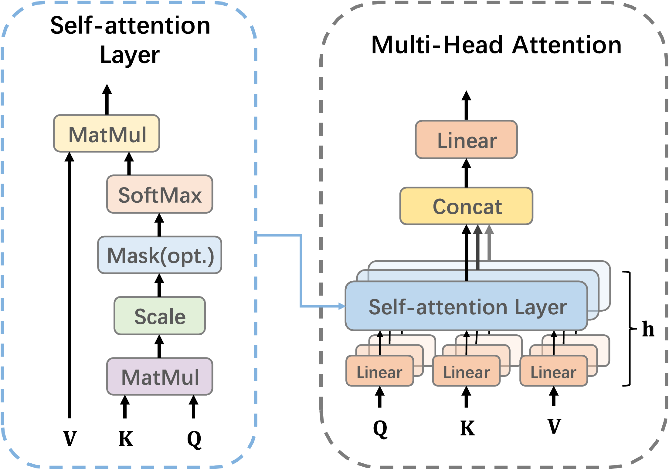
The input sequence is mapped into h different vector subspaces through linear transformations, producing h sets of Q i , K i , and V i . Each attention head independently computes its attention weights and applies them to the sequence, resulting in independent attention outputs. Multi-head attention as shown in Figure 4, improves the model’s ability to capture complex relationships in the data.
The multi-head attention mechanism.

Figure 4. Long description
A diagram of the multi-head attention mechanism. The diagram is divided into two main sections: Self-attention Layer and Multi-Head Attention. The Self-attention Layer section shows a sequence of operations starting with three inputs labeled Q, K, and V. These inputs undergo matrix multiplication (MatMul), followed by scaling, an optional masking step, and a softmax function. The output of the softmax function is then subjected to another matrix multiplication. The Multi-Head Attention section, as shown in Figure 4, depicts multiple self-attention layers operating in parallel, each receiving linear transformations of the Q, K, and V inputs. The outputs of these self-attention layers are concatenated and passed through a linear transformation. The diagram illustrates the flow of data through these layers, highlighting the parallel processing of multiple attention heads.
Feedforward Network: Comprising two fully connected layers, the feedforward network follows the multi-head attention mechanism and applies further nonlinear transformations to enhance the model’s expressive power.
Residual Connection: The input is directly added to the output, helping prevent the vanishing gradient problem and improving training performance.
Loss Function: To evaluate the proposed method, we use MSE as the loss function, defined as:
 \begin{equation} L=\frac{1}{n} \sum\limits_{i=1}^{n}\big(y_{i}-\overset{\wedge }{y_{i}}\big)^{2} \end{equation}
where n is the number of samples,
 $y_{i}$
is the true value, and
 $\overset{\wedge }{y_{i}}$
is the predicted value.
Optimizer: The Adam optimizer is used to update model parameters, combining momentum and adaptive learning rates for faster convergence during training.
The model is trained over multiple iterations with masked input data. Loss is calculated, parameters updated, and performance evaluated using a validation set to fine-tune hyperparameters for optimal results.
3. Experiment and result
3.1. Datasets
There are two datasets used in this paper to assess the model’s generalization. Dataset A is the INR 18650-20R battery dataset from the University of Maryland, which includes four typical driving conditions [32]:
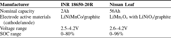
Main battery parameters.

Table I. Long description
A table comparing main parameters of two battery types, INR 18650-20R and Nissan Leaf. The table has 4 rows and 3 columns. Column headers are Manufacturer, INR 18650-20R, and Nissan Leaf. Row labels are Nominal capacity, Electrode active materials (cathode/anode), Voltage range, and SOC range. Row 1: Nominal capacity, 2Ah, 56Ah. Row 2: Electrode active materials (cathode/anode), LiNiMnCo/graphite, LiMn2O4 with LiNiO2/graphite. Row 3: Voltage range, 2.5-4.2V, 2.6-4.2V. Row 4: SOC range, 0-80 percent, 0-96 percent.
Schematic of battery testing with Nissan Leaf.

DST (Dynamic Stress Test): Evaluates extreme condition performance (3C rapid charge/discharge, 45°C ambient)
FUDS (Federal Urban Driving Schedule): Characterizes urban driving patterns with frequent
 $\lt$
2C load variations
US06 (Supplemental FTP Cycle): Simulates highway driving with sustained
 $ \gt$
2C discharge rates
BJDST (Beijing Driving Schedule Test): Represents composite urban–rural driving with stochastic 0.5–2.5C load fluctuations
Dataset B is established by collecting data from Nissan Leaf batteries. The experimental setup is shown in Figure 5. Retired Nissan Leaf batteries were used to collect charge and discharge data. The setup includes a battery pack of 16 cells, with the I-tech tester recording key parameters such as voltage, current, and temperature. To assess the model’s generalization, the publicly available INR 18650-20R dataset from the University of Maryland was also used for comparison. Table I lists the main parameters of both battery types.
The charge and discharge cycles followed a 7-day cycle, adjusted using the Day-Ahead and Real-Time Energy Timing Shift [Reference Yang, Ling, Li, Han and Tong33]. The charging strategy was dynamically modified based on day-ahead and real-time energy demand fluctuations to simulate real-world usage. This approach ensured the experimental data’s relevance and applicability.
3.2. Comparative methods
An Abstract is required for every paper; it should succinctly summarize the reason for the work. This study applied various SOC prediction methods to highlight the effectiveness and superiority of the proposed approach. The methods used were:
-
1. Deep neural networks (DNN)
This study uses a DNN with four hidden layers to predict the battery SOC, with a single neuron at the output for SOC prediction.
-
2. Convolutional neural networks (CNN)
A CNN is used for SOC prediction, consisting of three convolutional layers with 32, 64, and 128 filters, two fully connected layers with 256 and 128 neurons, and three pooling layers with a pool size of 2.
-
3. Long short-term memory network model
An LSTM model with two 128-neuron layers and a fully connected layer is used for SOC prediction, leveraging its ability to capture long-term dependencies in time series data.
-
4. Transformer
A Transformer-based model, comprising an input layer, position encoding, multi-head attention, feedforward network, and output layer, is designed to predict the battery SOC trend accurately.
3.3. Nissan Leaf battery data tests
To ensure accurate and reliable predictions, results are averaged over multiple trials to reduce randomness. The study uses five tasks to evaluate different methods on the Nissan Leaf lithium-ion battery dataset. Each task involves 10 batteries, with 20 discharge segments in total. Four segments are randomly selected for testing, and the rest are used for training. Tasks T1 through T5 independently assess the methods’ performance across various battery discharge stages. Each task undergoes five independent trials per battery, with results averaged for consistency and reliability.
Figure 6 illustrates that the lithium-ion battery SOC prediction model proposed in this study outperforms the DNN, CNN, LSTM, and Transformer models in terms of prediction accuracy. In the red box, the proposed method achieves the smallest prediction error, with a root mean square error (RMSE) of 0.0012, whereas the RMSEs for the other methods are 0.0011, 0.0064, 0.0026, and 0.0016, respectively. In the blue box, the proposed method shows the largest prediction error at 0.0042, while the RMSEs for the other models are 0.0072, 0.0044, 0.0060, and 0.0069. Overall, the proposed model demonstrates superior accuracy in SOC prediction, outperforming the other methods in both the smallest and largest error cases.
Figure 7 presents the comparison of different networks in the T4-2 task. As shown in the red box, the proposed method achieves the smallest prediction error, with an RMSE of just 0.0008, significantly better than the other four methods, whose RMSEs are 0.0097, 0.0098, 0.0055, and 0.0030, respectively. In the blue box, although the proposed method exhibits the highest prediction error with an RMSE of 0.0035, it still outperforms all models except for the Transformer, whose RMSE is 0.0041. The RMSEs for the other methods are 0.0063, 0.0083, and 0.0127, respectively. This further confirms the superiority of the proposed method for SOC prediction.
Comparison of prediction results from different networks in task T2-1.

Figure 6. Long description
The image contains one main line graph and two inset line graphs. The main graph shows the SOC percentage over time in minutes, comparing the true values with predictions from various models: CNN, DNN, LSTM, Transformer, and Masked Transformer model. The x-axis represents time in minutes, ranging from 0 to 80, and the y-axis represents SOC percentage, ranging from 0 to 60. The true values are depicted in red, while the predictions from the different models are shown in various colors: CNN in yellow, DNN in gray, LSTM in brown, Transformer in light blue, and Masked Transformer model in dark blue. The main graph highlights two regions with dashed boxes, indicating areas of interest that are zoomed in on the inset graphs. The first inset graph, located in the upper left, zooms in on the time range from 0 to 10 minutes and SOC range from 48 to 56 percent. The second inset graph, located in the lower right, zooms in on the time range from 40 to 50 minutes and SOC range from 15 to 20 percent. These inset graphs provide a closer look at the performance of the different models in these specific time intervals. The overall trend shows a decrease in SOC over time, with the different models closely following the true values but with some variations.
Comparison of prediction results from different networks in task T4-2.

Figure 8 highlights the model’s performance in SOC prediction. In the T5-4 task, the proposed method achieves the smallest prediction error, with an RMSE of 0.0017, significantly outperforming the other four methods, whose RMSEs are 0.012, 0.0067, 0.0135, and 0.0038, respectively, as shown in the red box. In the blue box, although the proposed method reaches the highest prediction error, it still outperforms the other methods, whose RMSEs are 0.0162, 0.0107, 0.0045, and 0.0041. These results further confirm the effectiveness and superiority of the proposed method in SOC prediction.
Comparison of prediction results from different networks in task T5-4.

Figure 8. Long description
The image contains one main line graph and two inset line graphs. The main graph shows the state of charge (SOC) percentage over time in minutes. The x-axis is labeled ‘Time (min)’ and ranges from 0 to 80 minutes. The y-axis is labeled ‘SOC (%)’ and ranges from 0 to 50 percent. The inset graphs provide zoomed-in views of specific time intervals. The first inset graph focuses on the time range from 0 to 10 minutes, and the second inset graph focuses on the time range from 0 to 8 minutes. Each graph includes multiple lines representing different prediction methods: true, DNN, CNN, LSTM, Transformer, and Masked Transformer model. The lines show the SOC percentage predicted by each method over time. The main graph highlights the overall trends and differences in prediction accuracy among the methods. The inset graphs provide detailed views of the initial time periods, showing how closely each method’s predictions align with the true SOC values. The lines are color-coded according to the legend at the top of the main graph. The main graph shows that the true SOC decreases steadily over time, while the predictions from different methods vary in their accuracy and alignment with the true SOC. The inset graphs reveal more detailed differences in the initial predictions, with some methods showing closer alignment to the true SOC than others.
Figure 9 illustrates the RMSE comparison across different tasks. Except for tasks T1-3, T2-4, T3-3, and T4-1, where the RMSE is slightly higher than that of the Transformer model, the proposed method outperforms the DNN, CNN, LSTM, and Transformer models in the remaining 16 tasks. These findings further highlight the superior prediction performance of the proposed method in the majority of tasks.
RMSE of SOC prediction results under different tasks.

In summary, the proposed model demonstrates superior performance compared to baseline methods across all evaluation metrics, with consistently lower RMSE values indicating enhanced prediction accuracy. These results suggest that our Transformer-based SOC estimation approach represents a robust solution for the target application scenarios. However, the prediction accuracy exhibits relative degradation within the 10–30% SOC range, highlighting a critical challenge for future research to address. This limitation may be attributed to the characteristic voltage plateau effects in lithium-ion batteries during low-charge states.
3.4. INR 18650-20R battery data tests
This section defines four tasks to assess the performance of various methods on the INR 18650-20R lithium-ion battery dataset. Each task consists of six discharge data segments: three with SOC ranges from 0% to 80%, and three with SOC ranges from 0% to 50%. For each task, two segments from the 0–80% SOC range and two from the 0–50% SOC range are used for training, while the remaining data are used for testing. By independently predicting using test data from different operating conditions, the performance and predictive capabilities of the methods on this dataset are thoroughly evaluated. To better illustrate the results, we selected four different sub-intervals from the entire discharge curve for each operating condition and plotted them in four separate graphs. Each graph displays the performance of different models within the corresponding interval, allowing for a clearer comparison of the RMSE values across models in different intervals.
The BJDST condition simulates the battery’s charging and discharging in real-world driving, covering a range of scenarios like low-speed cruising and dynamic events such as rapid acceleration and braking. This makes it an ideal case for testing SOC prediction models under diverse load conditions. As shown in Figure 10, the proposed method achieves the smallest RMSE of 0.0010, outperforming other models with RMSEs of 0.0045, 0.0025, 0.0035, and 0.0031. Even at its largest RMSE of 0.0028, it still outperforms the other models, which have RMSEs of 0.0072, 0.0035, 0.0038, and 0.0054.
SOC prediction results under BJDST working condition.

The DST condition simulates battery performance under high-load, fast charging, and discharging conditions to assess its stability and reliability in extreme operations. It involves frequent high-power cycles, leading to significant SOC changes. As shown in Figure 11, the proposed method achieves the smallest RMSE of 0.0007, outperforming the other models with RMSEs of 0.0029, 0.0061, 0.0030, and 0.0027. In contrast, the proposed method’s maximum RMSE of 0.0035 is better than the others, with RMSEs of 0.0080, 0.0041, 0.0041, and 0.0031. These results confirm the proposed method’s exceptional performance under extreme conditions.
SOC prediction results under DST conditions.

Figure 11. Long description
Four line graphs depict the state of charge (SOC) prediction results under different dynamic stress test (DST) conditions. Each graph compares the performance of various prediction methods, including true values, convolutional neural network (CNN), deep neural network (DNN), long short-term memory (LSTM), transformer, and masked transformer model. Panel DST#1-1: The line graph shows SOC percentage on the vertical axis and time in minutes on the horizontal axis. The true values are represented by a red line, while other methods are depicted in different colors. The inset zooms in on a specific time range for detailed comparison. Panel DST#1-2: Similar to Panel DST#1-1, this line graph shows SOC percentage over time with an inset focusing on a particular time segment. Panel DST#1-3: This line graph also displays SOC percentage over time, with an inset highlighting a specific time interval. Panel DST#1-4: The final line graph presents SOC percentage over time, with an inset providing a closer look at a certain time range. Each panel includes a red dashed box indicating a region of interest for detailed analysis.
The US06 condition simulates highway driving and evaluates the battery’s performance under high-speed driving and aggressive acceleration. These conditions cause significant load changes and rapid SOC fluctuations, requiring precise prediction models. As shown in Figure 12, the proposed method achieves the lowest RMSE of 0.0011, outperforming the other models with RMSEs of 0.0021, 0.0059, 0.0025, and 0.0021. Even at its maximum RMSE of 0.0019, it outperforms the others, with RMSEs of 0.0030, 0.0042, 0.0068, and 0.0029. These results validate the proposed method’s superiority and reliability under high-load conditions.
SOC prediction results under US06 conditions.

The FUDS condition simulates urban driving, mainly testing the battery’s SOC changes during frequent acceleration, braking, and low-speed driving. These conditions cause frequent load fluctuations, requiring SOC prediction models to respond dynamically to rapid changes. As shown in Figure 13, the proposed method achieves the smallest RMSE of 0.0011, outperforming the other models with RMSEs of 0.0040, 0.0094, 0.0058, and 0.0037. Even at its maximum RMSE of 0.0031, it still outperforms the other models, which have RMSEs of 0.0101, 0.0065, 0.0078, and 0.0063. These results confirm the proposed method’s superiority and stability in urban driving conditions with frequent load changes.
SOC prediction results under FUDS conditions.

Figure 13. Long description
Four line graphs depict the State of Charge (SOC) prediction results under Federal Urban Driving Schedule (FUDS) conditions. Each graph represents different FUDS scenarios labeled as FUDS#1-1, FUDS#1-2, FUDS#1-3, and FUDS#1-4. The x-axis represents time in minutes, ranging from 0 to 15 minutes. The y-axis represents the SOC in percent, with varying ranges for each graph: 64 to 72 percent for FUDS#1-1, 50 to 56 percent for FUDS#1-2, 42 to 50 percent for FUDS#1-3, and 20 to 28 percent for FUDS#1-4. Each graph includes multiple lines representing different prediction methods: true, CNN, DNN, LSTM, Transformer, and Masked Transformer model. Insets in each graph zoom in on specific time intervals to highlight detailed differences among the prediction methods. The lines show varying degrees of alignment with the true SOC values, indicating the performance of each method under different driving conditions.
As shown in Figure 14, the RMSE values for various methods under different conditions are compared. The self-supervised model proposed in this paper outperforms the other four models in all conditions, consistently achieving lower RMSE values. It demonstrates the highest prediction accuracy, particularly in complex load and extreme conditions, effectively responding to SOC fluctuations and delivering precise predictions. In comparison, the DNN and CNN models exhibit higher RMSE values, indicating suboptimal performance. Although the Transformer and LSTM models perform well, they are still outperformed by the proposed self-supervised model. These results confirm the exceptional performance of the self-supervised model, proving its effectiveness and reliability in battery SOC prediction.
RMSE of SOC prediction results under different working conditions.

4. Conclusion
The self-supervised SOC prediction model proposed in this study performs outstandingly under various conditions in both the Nissan Leaf lithium-ion battery dataset and the INR 18650-20R battery dataset, offering significant advantages over traditional methods such as DNN, CNN, LSTM, and Transformer. In tasks involving the Nissan Leaf lithium-ion battery dataset, the proposed method consistently achieves low RMSE, demonstrating superior prediction accuracy. In both minimum and maximum error cases, the proposed method outperforms the other models, particularly in handling complex SOC variations, offering precise predictions.
Similarly, in the INR 18650-20R battery dataset, the proposed model excels under all four test conditions. It consistently maintains low RMSE, particularly under complex and extreme conditions, effectively predicting SOC changes and demonstrating its robustness and stability in diverse scenarios.
Overall, the proposed method demonstrates superior predictive capabilities across a range of conditions, confirming its effectiveness and reliability for battery SOC prediction.
Author contribution
Wei Zhang contributed to conceptualization, methodology, and formal analysis and provided supervision; Letian Niu developed the software, performed validation and formal analysis, and wrote the original draft; Shaojie Yang was responsible for data curation, investigation, and resources; Xiang Li handled writing review and editing, project administration, and funding acquisition.
Financial support
The material in this paper is based on work supported by the Ministry of Education of China under Grant (HKZY20220429).
Competing interests
The authors declare no conflicts of interest.
Ethical standards
Not applicable.