1 Limitations of numerical simulations

Numerical simulations help us understand how real pulsars work. Unfortunately, they have severe limitations.

1.1 Lego™ tiles

The radius of a neutron star is about 10 km. The light cylinder lies a few to a few thousand times away. The polar cap is a few to a hundred times smaller. It is thus very hard to equally resolve in three dimensions the stellar vicinity and the magnetosphere over several light cylinder radii, with the possible exception of millisecond pulsars. The current state-of-the-art three-dimensional (3D) numerical resolution consists of at most a few hundred grid cells in each direction inside the light cylinder. This is manifestly insufficient to capture and resolve certain important features of the pulsar magnetosphere that are seen in high-resolution two-dimensional (2D) solutions. Ten years ago, Timokhin (Reference Timokhin2006) analysed the axisymmetric pulsar magnetosphere in the highest yet achieved resolution of more than 10 000 grid cells inside the light cylinder. Even though that resolution is not sufficient to resolve the internal structure of the current sheet, it taught us a couple of interesting things about the magnetospheric Y-point (the tip of the corotating, so-called ‘dead’, zone) that are hard to see in 3D simulations.

1. (i) The poloidal magnetic and electric fields right above and below the Y-point both drop to zero. Thus, the charge density at the Y-point also drops to zero (see also Uzdensky Reference Uzdensky2003).

2. (ii) In the ideal magnetohydrodynamic (MHD) solution (Contopoulos, Kazanas & Fendt Reference Contopoulos, Kazanas and Fendt1999, hereafter CKF), the current sheet extends inwards of the Y-point along the boundary (separatrix) of the dead zone. In that region, the current sheet is charged oppositely to the charge of the equatorial current sheet, and its charge density changes discontinuously to zero at the Y-point. In particular, as the Y-point approaches the light cylinder, the electric and magnetic fields and the charge density right interior to it diverge (Uzdensky Reference Uzdensky2003; Kalapotharakos & Contopoulos Reference Kalapotharakos and Contopoulos2009).

These features of the current sheet are completely lost in current 3D numerical simulations. What is most disconcerting, is that in order to determine the pulsar energy losses, that is, its spindown rate, we need to know the position of the Y-point since this is what determines how many field lines remain closed in the dead zone, and how many carry electromagnetic radiation. In numerical simulations that begin with a stationary star that is then set to uniform rotation, it has been observed that magnetic field lines open up after a fraction of one stellar rotation and a Y-point forms initially at some distance $r_{Y}$ inside the light cylinder (the cylindrical radius $r_{LC}\equiv c/{\it\Omega}$ , where ${\it\Omega}$ is the stellar rotational angular velocity). When that happens, the solution settles to a perfectly valid (‘happy’) steady state that emits electromagnetic energy at a rate $L(r_{Y})\approx (r_{Y}/r_{LC})^{-2}L(r_{LC})>L(r_{LC})$ (Contopoulos Reference Contopoulos2005; Timokhin Reference Timokhin2006). The Y-point then gradually evolves towards the final steady state where the Y-point reaches the light cylinder. Depending on the numerical resolution, that evolution takes place at a much longer timescale (several rotational periods) than the timescale (fraction of one period) needed for the original happy steady state to establish itself. Note that, in practice, the Y-point is determined as the innermost tip of the equatorial current sheet where it reaches the corotating dead zone.

This may very well be a serious problem in the numerical determination of the pulsar spindown rate. What we are really interested to know is $L(r_{LC})$ because we believe that as the pulsar spins down, the corotating dead zone manages to always lie close to the instantaneous light cylinder, thus $r_{Y}\approx r_{LC}$ . This is achieved via continuous reconnection at the Y-point through which more and more formerly open field lines close and increase the size of the dead zone. 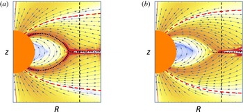If that is not the case, and during the small amount of time available to run our numerical simulation the magnetosphere has relaxed to an $r_{Y}$ significantly different from $r_{LC}$ (see figure 1; compare also to figure 3 of Philippov, Spitkovsky & Cerutti Reference Philippov, Spitkovsky and Cerutti2015), then the numerical estimate of the spindown luminosity $L(r_{LC})$ is unreliable. Note that, in reality, $r_{Y}$ may not keep up with the light cylinder as the pulsar spins down, and this may account for the measured values of pulsar braking indices that are found to be less than the canonical value of three (see also Kundt Reference Kundt1998, for an alternative view). The numerical evaluation of the real pulsar braking index is, however, way beyond the capabilities of modern computers.

Figure 1.

Examples of ideal MHD numerical simulations with Y-points clearly inside the light cylinder. These particular simulations run only for six stellar rotations which apparently was not enough time for them to relax to a final steady state. Vertical dashed line: line cylinder. Lines with arrows: poloidal magnetic field. Colour scale: magnitude of poloidal electric current density multiplied by $R^{2}$ (white regions: no poloidal currents; red regions: poloidal current sheets, also drawn with black dotted lines). The lines of zero poloidal electric current that separate the regions of outgoing and ingoing electric currents are shown with red short dashed lines (see also figure 2). Orange semicircle: neutron star. (a): Here $E$ is enforced to be less than $B$ everywhere. In practice, this implies that current sheets are treated as contact discontinuities. Both the equatorial and separatrix current sheets form. The equatorial current sheet extends clearly inside the light cylinder. The current sheet appearing inside the Y-point is clearly an artefact of our particular treatment of contact discontinuities. (b): We allow $E$ to take any value compared we $B$ , and current sheets are treated with a dissipative Aristotelian prescription (Gruzinov Reference Gruzinov2013). In that case, only the equatorial current sheet survives, and the separatrix current sheet disappears, as expected in Contopoulos, Kalapotharakos & Kazanas (Reference Contopoulos, Kalapotharakos and Kazanas2014), and seen also very clearly in figure 3 of Cerutti et al. (Reference Cerutti, Philippov, Parfrey and Spitkovsky2015a ).

2 What drives magnetospheric dissipation?

Let us remind the reader how we arrived at our current understanding of the pulsar magnetosphere. The basic picture of a unipolar inductor was formulated by Goldreich & Julian (Reference Goldreich and Julian1969) and a cartoon of the magnetospheric structure was drawn. In that picture, electric charges fill and electric currents flow through the magnetosphere, in such a way that an outward $\boldsymbol{E}\times \boldsymbol{B}$ Poynting flux vector develops everywhere. Another fact that was obvious from the very first discussion on pulsar magnetospheres is that the magnetosphere, if ideal, must open up beyond a distance from the axis of rotation known as the light cylinder. Obviously, a poloidal magnetic field discontinuity must inevitably form beyond the light cylinder (as is shown in the original Goldreich–Julian cartoon), but that is not too important since the poloidal magnetic field drops very fast with distance from the light cylinder.

What is much more important is an equatorial discontinuity in the azimuthal magnetic field, that is, the existence of an equatorial poloidal current sheet. The first to theorize this configuration was Lyubarskii (Reference Lyubarskii1990), and this led to a very important school of thought that the acceleration of the pulsar wind may in fact take place in the equatorial poloidal current sheet (Lyubarsky & Kirk Reference Lyubarsky and Kirk2001). However, his original argument for the existence of such a current sheet was based on a study of an artificial solution up to (and not beyond) the light cylinder consisting of field lines that close some distance inside the light cylinder, and field lines that reach the light cylinder. Obviously, at that time it was completely uncertain what the latter field lines would do beyond the light cylinder, and unless a global solution was obtained, no one was in a position to know with confidence whether such an equatorial poloidal current sheet existed or not.

That solution appeared 30 years later (CKF) and was for several years met with caution and disbelief (Ogura & Kojima Reference Ogura and Kojima2003). Current sheets are usually unstable in nature, so the equatorial current sheet that CKF obtained was thought to be artificial. A few authors tried to refute our discovery proposing various other solutions without current sheets, but all such efforts did not seem to represent real pulsar magnetospheres (Lovelace, Turner & Romanova Reference Lovelace, Turner and Romanova2006; Beskin Reference Beskin2010). Only after Spitkovsky (Reference Spitkovsky2006) reproduced our solution as the final steady state (after 20 rotations) of a time-dependent numerical evolution did the community begin to pay attention to the possibility that the equatorial poloidal current sheet discovered by CKF may be an integral and most important part of the pulsar magnetosphere. Spitkovky’s numerical results have since then been confirmed by several others (McKinney Reference McKinney2006; Kalapotharakos & Contopoulos Reference Kalapotharakos and Contopoulos2009; Tchekhovskoy, Spitkovsky & Li Reference Tchekhovskoy, Spitkovsky and Li2013).

However difficult the numerical problems associated with the equatorial current sheet may be (see the previous section), we cannot ignore it. An important point that we tried to emphasize during a series of three short papers that we wrote many years ago (Contopoulos Reference Contopoulos2007a ,Reference Contopoulos b ,Reference Contopoulos c ) is that one cannot say anything about pulsars without taking proper account of the equatorial current sheet. As we argued in the previous section, pulsars do not shoot energetic beams on their own. Pulsar magnetospheres are global structures that are characterized by what happens both on the surface of the star (the magnetic field structure, the rotation rate, and the availability or non-availability of charge carriers there), and at the equatorial current sheet that develops way out in the magnetosphere, and not by the boundary conditions at ‘infinity’ (as long as the system is able to establish super Alfvènic radiation conditions ( $\boldsymbol{E}\times \boldsymbol{B}/B^{2}\rightarrow \hat{\boldsymbol{r}}$ at large distances). In particular, if the physical conditions in the current sheet preclude any dissipation there, the current sheet establishes itself as a contact discontinuity with $\boldsymbol{B}$ parallel to it above and below it. This was the case for CKF and all subsequent ideal MHD simulations. Physically, this implies that the magnetosphere is able to supply the electric charge carriers needed to support the electric charge density and electric current density required by the ideal MHD solution. As long as the required charges are freely supplied, there is no ‘residual’ electric field along the current sheet that would lead to particle acceleration along the current sheet and/or reconnection.

At this point, we would like to describe briefly what takes place along the equatorial current sheet. As we said, in a contact discontinuity the magnetic field is parallel to it above (let us denote it with $\boldsymbol{B}_{\Vert CS}$ ), reverses direction inside the current sheet, and becomes equal in magnitude and antiparallel below. At the same time, the electric field is perpendicular to it above the current sheet (let us denote it with $\boldsymbol{E}_{\bot CS}$ ), reverses direction and points in the opposite perpendicular direction below, thus the current sheet is obviously charged with surface electric charge density

(2.1) $$\begin{eqnarray}{\it\sigma}=\frac{E_{\bot CS}}{2{\rm\pi}}.\end{eqnarray}$$

Note that $E_{\bot CS}=(r/r_{LC})B_{r}$ above the current sheet. In this picture, there is no ‘residual’ electric field along the current sheet. Such a field component (let us denote it with $\boldsymbol{E}_{\Vert CS}$ ) would appear only if the magnetosphere above and below the current sheet is driven to converge towards it with convergence velocity

(2.2) $$\begin{eqnarray}v_{converge}\equiv \frac{\boldsymbol{E}_{\Vert CS}\times \boldsymbol{B}_{\Vert CS}}{B^{2}}c.\end{eqnarray}$$

Note that $\boldsymbol{E}_{\Vert CS}$ lies along the direction of the electric current in the current sheet, hence it is perpendicular to $\boldsymbol{B}_{\Vert CS}$ , and continuous (in the same direction) above and below the current sheet ( $\boldsymbol{E}_{\Vert CS}$ becomes radial, $\Vert \hat{\boldsymbol{r}}$ , in the current sheet midplane). This is often called the reconnection electric field, and in the ideal MHD region right above and below the current sheet, $E_{\Vert CS}=(r/r_{LC})B_{z}$ . Why this is non-zero depends of course on the global structure of the magnetosphere. On the other hand, this is what dictates the dissipation rate at the current sheet, which is obviously related to the microscopic conditions in the current sheet. So the ‘chicken and egg’ question is:

Is it the global magnetospheric structure that redirects electromagnetic Poynting flux towards the equator, or the local reconnection and plasma acceleration that dissipates energy in the current sheet?

In a steady state, a balance will be achieved between the Poynting flux $\boldsymbol{E}_{\Vert CS}\times \boldsymbol{B}_{\Vert CS}$ entering the current sheet and the effective dissipation rate ${\it\eta}E_{\Vert CS}^{2}$ in the current sheet (we have defined here an effective dissipation parameter ${\it\eta}$ such that $J_{CS}=E_{\Vert CS}/{\it\eta}$ ). Thus, the residual electric field in the current sheet is equal to

(2.3) $$\begin{eqnarray}E_{\Vert CS}=\frac{2{\it\eta}}{lc}B_{\Vert CS}\equiv \frac{2}{{\mathcal{R}}_{m}}B_{\Vert CS},\end{eqnarray}$$

where $l$ is the thickness of the current sheet and ${\mathcal{R}}_{m}$ is the associated magnetic Reynolds number (or Lundquist number) based on $l$ and the speed of light. Unfortunately, this does not answer our question of what determined the dissipation rate. As we will see next, localized numerical simulations alone can only yield a partial answer to this question.

The magnetosphere can in principle establish a CKF-type equilibrium with a dissipationless current sheet, where all magnetic field lines that cross the light cylinder open up to infinity. In practice, localized numerical simulations have shown that, even without external driving, such a current sheet becomes unstable to relativistic Petschek reconnection (Sironi, Spitkovsky & Arons Reference Sironi, Spitkovsky and Arons2013). A finite reconnection speed $v_{converge}\sim 0.1c$ is established which corresponds to the maximum possible inflow speed for that particular type of reconnection, namely $v_{maxPetschek}\approx ({\rm\pi}/8\ln {\mathcal{R}}_{m})c$ (i.e. the reconnection electric field is practically independent of the local conditions in the current sheet; see, e.g. Cowley (Reference Cowley and Priest1985)). This is a local property of the current sheet, and in that case a global magnetospheric configuration establishes itself such that $v_{converge}^{2}+v_{\Vert CS}^{2}\approx c^{2}$ , or equivalently

(2.4) $$\begin{eqnarray}B_{r}/B_{z}\sim 9.95\end{eqnarray}$$

right above and below the equatorial current sheet. Here, $v_{\Vert CS}\equiv (E_{\bot CS}/B_{\Vert CS})c$ is defined as the drift velocity parallel to the current sheet just above and below it. As estimated in (2.4), the entry angle of magnetic field lines into the equatorial current sheet is very small, hence only a small amount of magnetospheric Poynting flux enters and is dissipated into the current sheet.

Another way to understand this configuration is to consider the analogy with an infinite infinitely thin plane conductor threaded by a uniform current distribution. In that case, a topology of uniform and opposite direction magnetic field $B_{\Vert }$ forms above and below the plane. The source of the field is the current sheet electric current. If we remove all external power sources and consider that the sheet is a non-ideal conductor with effective dissipation ${\it\eta}$ , then the current will begin to die out, the current sheet will absorb electromagnetic energy from above and below, and the electric current will continue to flow as long as the magnetic field reservoir is not depleted (i.e. as long as there exist a magnetic field above and below the plane). In that case, the driver of magnetospheric dissipation is the local dissipation rate in the equatorial current sheet.

We are a little concerned here that Petschek-type reconnection cannot proceed for too long. As is seen in numerical simulations, closed magnetic field islands form along the current sheet, and when the whole current sheet layer is filled with such islands, the process of tearing and island formation will not proceed any longer and that particular type of reconnection will saturate. This does not preclude of course the occurrence of random strong localized energetic reconnection events along the current sheet which may yield powerful flashes of high-energy and/or radio emission (Cerutti et al. Reference Cerutti, Werner, Uzdensky and Begelman2013, Reference Cerutti, Werner, Uzdensky and Begelman2014). If our concern is justified then, however exciting the results of localized current sheet particle-in-cell (PIC) numerical simulations may be, they do not represent what really goes on in steady state in the pulsar magnetosphere. In fact the latest ‘ab initio’ global magnetospheric simulations yield values of $B_{r}/B_{\bot }$ much smaller than 9.95 (of the order of unity near the light cylinder).

On the other hand, there is strong indirect evidence that strong dissipation does take place in the current sheet (e.g. Gruzinov Reference Gruzinov2014; Kalapotharakos, Harding & Kazanas Reference Kalapotharakos, Harding and Kazanas2014; Cerutti, Philippov & Spitkovsky Reference Cerutti, Philippov and Spitkovsky2015b ). So, how is the current sheet forced and how much? PIC numerical simulations do help, provided we have a clearer idea of how to interpret them. So, let us now consider an important feature of the equatorial current sheet, the so-called Y-point, that may hold the answer to its vertical forcing.

3 The Y-point

Current sheets have a thickness comparable to the gyro-radius of the particles that support their electric current. It is well known that these particles follow meandering (snake) orbits and if a reconnecting electric field exists along the current sheet (i.e. if there is dissipation), these particles are accelerated along the direction of $E_{\Vert CS}$ following Spiser orbits, that is, meandering orbits that become narrower across and more stretched along the direction of acceleration. In the particular case of the pulsar equatorial current sheet this is true only for the main charge carrier of the current sheet, the one with the sign of charge of the charged sheet. This charge carrier is accelerated outwards. The other charge carrier is accelerated inwards, but in doing so it meanders all of the way to the outskirts (the surfaces) of the current sheet where the main $\boldsymbol{E}\times \boldsymbol{B}$ direction is still outwards. So, the meandering of the other charge carrier is ‘messy’, with excursions outside the current sheet. Nevertheless, on average, these too are accelerated inwards. However, it could be that they cannot survive for much time along the current sheet. This has already been seen in numerical simulations (Contopoulos Reference Contopoulos2007b ; Philippov et al. Reference Philippov, Spitkovsky and Cerutti2015), and remains to be confirmed with further studies.

The particle gyro-radius is determined by the particle kinetic energy perpendicular to the magnetic field. In the pulsar magnetosphere, the perpendicular kinetic energy is quickly radiated away through curvature radiation, and if most of the kinetic energy is radiated away, then the particle gyro-radius becomes smaller and smaller, and the current sheet narrower and narrower. In the limit of very small gyro-radius the current sheet can still be held from collapsing by its own electrostatic repulsion (see Contopoulos et al. (Reference Contopoulos, Kalapotharakos and Kazanas2014), for details). In other words, the current sheet will never completely collapse because it is held by its own electrostatic repulsion. This is true unless we sit right at the Y-point.

As we have argued before, the poloidal magnetic field, thus also the poloidal electric field and the electric charge density all three vanish right outside (but not inside) the Y-point. It becomes then extremely problematic to support a current sheet right outside the Y-point, unless of course the external magnetic pressure (i.e.  $B_{{\it\phi}}$ ) also vanishes at that point. This simple result has very strong implications for the global structure of the magnetosphere. First, this is equivalent to the vanishing of the electric current along the separatrix between the corotating dead zone and the open magnetosphere. There is no current sheet that returns to the star. The equatorial current sheet does not close the electric circuit onto the star. And if we do not allow for electric currents to flow through the Y-point, then the old CKF-type solution cannot be valid anymore, and the magnetosphere must find a new global equilibrium that is different from the CKF solution. In fact, we expect this equilibrium to be strongly dissipative in the current sheet for a simple reason: CKF argued that their solution is the only possible solution for a dissipationless ideal magnetosphere. The new solution is still ideal everywhere, but very different in the current sheet, thus also strongly dissipative there. The equatorial current sheet must be gradually replenished by the magnetospheric electric charges that both support it vertically and also form the electric current that threads it. In doing so, Poynting flux enters the current sheet, and this energy flux must find a way to dissipate in the current sheet through reconnection and particle acceleration (with ensuing emission of radiation). We have thus found the origin of the magnetospheric forcing of the current sheet, namely the inability of the electric current in the current sheet to cross the Y-point.

The magnetospheric Y-point is indeed a problematic place and several authors have studied it in detail in the past. It cannot approach too close to the light cylinder because in that case the corotation velocity at the tip of the dead zone would approach the speed of light and the magnetic and electric fields right inside it would diverge (Uzdensky Reference Uzdensky2003). At the same time, it must be in a position to support a sudden drop in its charge density. We will now present why we believe it is hard in practice for the Y-point to also support a continuous electric current through it. Before we proceed, let us here define as the ‘right’ type of particles, those that, when they move outwards, they support the magnetospheric electric current, and ‘wrong’ the other type. For example, in the case of the equatorial current sheet in the aligned rotator ( ${\it\Omega}$ parallel to the magnetic moment of the star), the positrons/protons/ions are of the ‘right’ type and electrons of the ‘wrong’ type.

In order to support at the same time a continuous current, a sudden density drop across, and a zero charge density just outside the Y-point, we must have two populations of particles that satisfy both

(3.1) $$\begin{eqnarray}{\it\rho}_{wrong}+{\it\rho}_{right}=0,\end{eqnarray}$$

and

(3.2) $$\begin{eqnarray}{\it\rho}_{wrong}v_{wrong}+{\it\rho}_{right}v_{right}=J_{Y}.\end{eqnarray}$$

However small the amount of dissipation in the equatorial current sheet (i.e. even if we just have spontaneous relativistic Petschek-type reconnection as shown in the localized numerical simulations of Sironi et al. Reference Sironi, Spitkovsky and Arons2013), then its electric field accelerates particles of the wrong type inwards. Therefore, $v_{wrong}$ is inward and particles of the wrong sign must follow inward meandering (snake) orbits traveling from outside the light cylinder into the Y-point. Unfortunately, this is not allowed topologically in a 3D magnetosphere (i.e. oblique rotator) for the following reason: outward moving particles of the right type do support a trailing (retarded) spiral current sheet (in the shape of a spinning ballerina’s skirt). Outside the light cylinder, particles cannot move inwards along such a 3D current sheet, thus ${\it\rho}_{wrong}$ must vanish outside the light cylinder. According to (3.2) $J_{Y}$ must also vanish there.

We are thus left with one possibility, namely a strongly dissipative equatorial current sheet with no electric current at the Y-point. This is the new standard magnetosphere of Contopoulos et al. (Reference Contopoulos, Kalapotharakos and Kazanas2014). We plan to investigate this solution in greater detail in the future. Meanwhile, let us go back to the old standard magnetosphere (CKF) and discuss certain of its features that have not been properly emphasized in the literature.

4 The crossings of the null surface

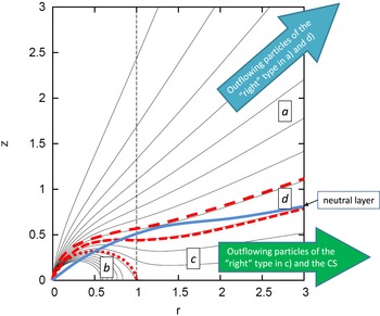
In the old standard magnetosphere, there is a line (in three dimensions, a surface) along which the Goldreich–Julian space charge density vanishes. This is the so-called null line (or null surface in three dimensions). In relation to the null line, there are four types of field lines (see figure 2).

1. (i) Open field lines that do not cross the null line. These originate on the stellar polar cap around the magnetic axis (which in axisymmetry coincides with the axis of rotation), and carry the main part of the polar cap poloidal electric current.

2. (ii) Closed field lines. All of them do cross the null line. These originate at low stellar latitudes up to the polar cap, and do not carry any poloidal electric current.

3. (iii) Open field lines that cross the null line once. These originate at the outskirts of the polar cap, and carry some fraction of the return poloidal electric current.

4. (iv) Open field lines that cross the null line twice. These originate somewhere inside the polar cap, and carry a very small amount of electric current of the same polarity as the main part of the polar cap.

Let us now consider each field line category and propose how it may be filled with charged particles. Note that the source of particles may very well be a stellar reservoir of protons (ions) and electrons, and does not need to resort to pair formation in magnetospheric gaps.

Figure 2.

The crossings of the null surface in the standard ideal force-free axisymmetric CKF magnetosphere. Vertical dashed line: the light cylinder. Blue line: null line (the neutral layer). The three red lines separate the four types of field lines (see the text for details). Type a: above the red long dashed line. Type b: below the red dotted line. Type c: between the red dotted and short dashed lines. Type d: between the red short and long dashed lines. The red short dashed line is the line of zero poloidal electric current $J_{CKF}$ (the electric current null line) that separates the magnetosphere into two regions of outgoing and ingoing electric currents respectively. For example, in the case of aligned pulsars, the ‘right’ type of particles are outflowing electrons in regions (a) and (d) (large blue arrow), and outflowing protons or positrons in region (c) and in the equatorial current sheet (CS; large green arrow). The electric charge and electric current null lines become one asymptotically (as $r\rightarrow \infty$ ).

The first type of field lines can very well be filled only with one type of particle, the one that we call ‘right’. In this part of the magnetosphere, the ‘right’ type can perfectly accommodate both the charge and electric current, namely ${\it\rho}={\it\rho}_{GJ}$ everywhere (in fact, almost everywhere as we will see next), and $J_{CKF}={\it\rho}_{GJ}v_{poloidal}$ . Following our definition of $J_{CKF}$ and $J_{GJ}$ in § 1.2, one can easily check that

(4.1) $$\begin{eqnarray}J_{CKF}<J_{GJ},\end{eqnarray}$$

near the stellar surface, and $J_{CKF}$ flows in the same direction as $J_{GJ}$ , hence only one type of charge carrier is sufficient to accommodate both the charge and electric current densities by adjusting the value of $v_{poloidal}<c$ , and

(4.2) $$\begin{eqnarray}J_{CKF}\rightarrow J_{GJ}\end{eqnarray}$$

at large distances, where $v_{poloidal}\rightarrow c$ . There is nothing terribly interesting to discuss in this region. There is a slight complication at the outskirts of this region where field lines at some point approach close to the null line, and at those positions the adjustment of $v_{poloidal}\equiv J_{CKF}/{\it\rho}_{GJ}$ does not work because the flow would become superluminal, but we will discuss this in relation to the field lines of the fourth type as defined above.

The second type of field lines does not have any problem whatsoever to be filled with two types of particles, positive and negative, that simply corotate with the star and thus form the so-called dead zone. Nothing is moving in the poloidal direction, and the poloidal electric current is zero. The particles are held in corotation by microscopic electric forces that are outside the realm of numerical ideal MHD analysis.

The third type of field line is much more interesting. These field lines start with the ‘wrong’ type of charge carriers on the stellar surface, and switch to the ‘right’ type beyond the null surface. Asymptotically, equation (4.2) still holds where $v_{poloidal}\rightarrow c$ . So these field lines need to at least carry just the Goldreich–Julian charge density at large distances. These particles of the ‘right’ type can very well originate on the stellar surface and support the electric current all of the way to the star. What needs to be done is to also pull the right amount of ‘wrong’ type particles from the stellar surface in order just to fill the region from the stellar surface up to the null line and some small distance beyond. In a configuration with the minimal possible number of particles, the innermost part of the third type of field lines contains a corotating region of the ‘wrong’ type of particles with density

(4.3) $$\begin{eqnarray}{\it\rho}_{corotating}\approx {\it\rho}_{GJ}-\frac{J_{CKF}}{c}.\end{eqnarray}$$

Obviously, since ${\it\rho}_{GJ}$ becomes zero some distance downstream along these lines, the corotating region of the ‘wrong’ type particles must extend some distance further downstream from the null line. We suspect that the region of corotating charge never extends beyond the light cylinder (where corotation is obviously not supported), and this is helped by the fact that $J_{CKF}\rightarrow 0$ at the boundary between regions three and four.

The fourth type of field lines is the most interesting of all. These carry an electric current which can very well be accommodated only by charge carriers of the ‘right’ type (which is the same type as the ‘right’ type for region one) since $J_{CKF}\rightarrow J_{GJ}$ at large distances, but consists of three regions of electric charge, of the ‘right’ type near the star and at very large distances, and of the ‘wrong’ type in between. The most economical obvious way to satisfy all of the requirements in this region is to increase the number density of particles of the ‘right’ type, and add a population of outflowing particles of the ‘wrong’ type which will adjust their poloidal velocities in order to build the in between region of the ‘wrong’ type Goldreich–Julian density. This configuration will extend also to the outskirts of region one in order to avoid superluminal velocities for particles of the ‘right’ type.

In any case, the poloidal speed of the charge carriers of the ‘wrong’ type will be much smaller than the speed of the charge carriers of the ‘right’ type. Thus, in regions three and four (extended also to the outskirts of region one), it is very natural to expect a configuration where a population of relativistic $v\approx c$ particles of one type flows through a large population of almost stationary particles of the other type. Such a configuration may naturally yield Cherenkov-type instabilities that may be related to the pulsar radio emission, as discussed, for example, in Lyutikov, Machabeli & Blandford (Reference Lyutikov, Machabeli and Blandford1999). This scenario certainly merits further investigation.

5 Epilogue

We have constructed a very economical pulsar magnetosphere consisting of large corotating regions filled with particles of one type of charge, threaded by streams of fast outflowing particles of the other type of charge. It is thus possible to fill the magnetosphere with a minimum amount of charge carriers by adjusting their speed and concentration that does not require continuous pair formation in the magnetosphere. In fact, particles of both negative and positive charge can naturally be found in the neutron star atmosphere with no need to resort to pair formation. Nature manages its resources wisely, so, instead of spending energy to produce a multitude of pairs, it can fill the magnetosphere with protons and electrons provided freely by the star. In that case, aligned rotators will obviously differ from counter-aligned ones. In particular, the equatorial current sheet of aligned pulsars will contain protons which will produce a markedly different high-energy signature than that of counter-aligned pulsars which contains electrons. Moreover, aligned pulsars will contain large corotating regions filled with electrons which may also produce a radio signal different from that of counter-aligned pulsars. Future observations may indeed be able to discriminate between aligned and counter-aligned pulsars.

We have also emphasized certain restrictions in the equatorial current sheet that may prevent it from extending all of the way to the stellar surface. The latter dramatically modify the structure of the pulsar magnetosphere away from the standard ideal MHD solution. Obtaining the new standard solution required the investigation of several magnetospheric issues in detail that cannot be reached in modern state-of-the-art 3D numerical simulations. The most recent numerical simulations yield vague hints that the magnetospheric structure is closer to the new standard solution, but are not yet in a position to reveal its details. We believe that it is too early to run global ‘ab initio’ magnetospheric PIC simulations since we need to understand in greater depth how the local conditions around the current sheet affect the global magnetospheric structure. Therefore, what we propose instead is to focus future PIC simulations in the study of the equatorial current sheet and the Y-point, and combine them with ideal MHD or FFE (force-free electrodynamic) simulations of the global magnetosphere.