1. Introduction
The Earth’s oceans are highly turbulent systems in complex domains with intricate external forcing mechanisms. Despite the various complications, the so-called geostrophic turbulence (Salmon Reference Salmon1998) at the meso- and large scales (from a few tens of km to a few thousand at the planetary scales) often forms semi-permanent, robust structures that persist over long periods that may range from weeks to several months. In some cases, the emergence of such quasi-steady states is strongly linked to two main dynamical factors (among several others). One of them is the Earth’s rotation, which constrains the horizontal motions to be at least one order of magnitude more intense than vertical motions (in the direction of gravity). A second factor is the dynamical effects on fluid motions as they transit over the spatially varying seafloor topography. The resulting quasi-two-dimensional behaviour due to both rotation and topography effects is the theoretical basis to address the problem of self-organisation and condensed states in several applications in geophysical fluid dynamics (Danilov & Gurarie Reference Danilov and Gurarie2000; van Heijst & Clercx Reference van Heijst and Clercx2009a ; Bouchet & Venaille Reference Bouchet and Venaille2012).
There are two motivations for this study. The first one is the observation of long-lived anticyclonic vortices in several mesoscale basins in the world’s oceans. Some well-known cases are the Lofoten vortex (Raj et al. Reference Raj, Chafik, Nilsen, Eldevik and Halo2015) and other anticyclones formed in similar North Atlantic basins (e.g. Solodoch, Stewart & McWilliams Reference Solodoch, Stewart and McWilliams2021). The Lofoten vortex has been known since the 1970s, and its formation and persistence have been the subject of several observational and numerical studies (e.g. Trodahl et al. Reference Trodahl, Isachsen, Lilly, Nilsson and Kristensen2020). However, there is evidence of cyclonic circulation at the rim of the Nordic Seas basins (Voet et al. Reference Voet, Quadfasel, Mork and Søiland2010). Moreover, robust cyclones also exist, such as in the Campeche Bay in the southwestern Gulf of Mexico (Vázquez De La Cerda et al. Reference Vázquez De La Cerda, Reid, DiMarco and Jochens2005). In this case, the vortex formation might be influenced by the predominant trade winds, which in this region have a positive curl (Zavala-Hidalgo et al. Reference Zavala-Hidalgo, Romero-Centeno, Mateos-Jasso, Morey and Martínez-López2014; Zavala Sansón Reference Zavala Sansón2019). Thus, a primary question is whether the essential dynamics of rotating flows over topographic depressions favours the formation of cyclones or anticyclones. The point is controversial because cyclonic circulations would be favoured over basins, according to the well-known tendency of oceanic flows to follow the geostrophic contours
 $f/h$
, with
 $f$
the Coriolis parameter and
 $h$
the fluid depth, with shallow water to the right (left) in the Northern (Southern) Hemisphere (Salmon Reference Salmon1998). This behaviour has been well known since the beginning of the last century (as illustrated by Isachsen et al. Reference Isachsen, LaCasce, Mauritzen and Häkkinen2003), and it has been measured in several regions of the world’s oceans (Holloway Reference Holloway2008).
A second motivation is understanding the emergence of quasi-steady or equilibrium states in two-dimensional (2-D) turbulence, particularly in closed domains (van Heijst & Clercx Reference van Heijst and Clercx2009b ). For decaying 2-D flows, the self-organisation process consists of the nonlinear energy transfer towards larger scales under the inverse energy cascade (Clercx, Maassen & Van Heijst Reference Clercx, Maassen and Van Heijst1999). As a result, the initially multiscale flow tends to form one or two large vortical structures that fill the domain (Brands, Maassen & Clercx Reference Brands, Maassen and Clercx1999; Maassen, Clercx & van Heijst Reference Maassen, Clercx and van Heijst2002). The vortex that emerges in a purely 2-D flow can rotate in either direction. That would also be the case for fluid columns over a flat bottom.
In the presence of rotating effects and topography, the dynamics is quasi-two-dimensional (Danilov & Gurarie Reference Danilov and Gurarie2000; Bouchet & Venaille Reference Bouchet and Venaille2012). In this case, the inverse energy cascade is arrested at the horizontal scale of the topographic variations, as the flow tends to follow the
 $f/h$
contours. The emergence of equilibrium states in geophysical fluid systems has been studied by applying methods of statistical mechanics, a behaviour first predicted for quasigeostrophic turbulence (Bretherton & Haidvogel Reference Bretherton and Haidvogel1976; Salmon, Holloway & Hendershott Reference Salmon, Holloway and Hendershott1976). Later studies have extended this framework to the more general shallow-water model (Merryfield, Cummins & Holloway Reference Merryfield, Cummins and Holloway2001; LaCasce, Nøst & Isachsen Reference LaCasce, Nøst and Isachsen2008; Zavala Sansón et al. Reference Zavala Sansón, González-Villanueva and Flores2010), and refined several aspects of the statistical arguments (Chavanis, Naso & Dubrulle Reference Chavanis, Naso and Dubrulle2010; Naso, Chavanis & Dubrulle Reference Naso, Chavanis and Dubrulle2011). The formation of currents along topographic contours has been demonstrated numerically in freely evolving flows over idealised basins (Cummins & Holloway Reference Cummins and Holloway1994; Wang & Vallis Reference Wang and Vallis1994), with more recent theoretical–numerical efforts focusing on the formation of semi-permanent vortices in isolated basins (Solodoch et al. Reference Solodoch, Stewart and McWilliams2021; LaCasce, Palóczy & Trodahl Reference LaCasce, Palóczy and Trodahl2024; Reinaud, LaCasce & Carton Reference Reinaud, LaCasce and Carton2025; Zavala Sansón Reference Zavala Sansón2025).
Another striking phenomenon is the self-organisation of geostrophic flows even in the presence of a random external forcing. In the oceanographic context, energy is injected into mesoscale motions via baroclinic instabilities (Salmon Reference Salmon1998). A different forcing (that will not be considered here) may be provided by the surface stress exerted by large-scale wind patterns over the ocean, which drive the formation of well-known large-scale structures like the subtropical gyres (e.g. the classical Stommel model), Fofonoff modes (Griffa & Salmon Reference Griffa and Salmon1989) or mesoscale vortices (Zavala Sansón et al. Reference Zavala Sansón, García-Martínez and Sheinbaum2023). A few studies examine the resulting flow when combining large-scale and random forcing functions (Griffa & Castellari Reference Griffa and Castellari1991; Zavala Sansón Reference Zavala Sansón2022).
In this paper, we study the long-term evolution of a turbulent flow in a closed basin with idealised experimental and numerical models. The chosen topography combines two quintessential features in 2-D and quasi-2-D turbulence: a central flat region and abrupt slopes around the domain. A primary question is whether the main ingredients of geostrophic turbulence (rotation, topography, forcing) favour the formation of cyclones or anticyclones in the basin. Two problems are examined: the decay of an initially disordered flow and the evolution of a randomly forced flow. The main results in both problems show (i) the robust development of steady mean currents cyclonically flowing over the topography around the domain, and (ii) a persistent anticyclonic vortex at the basin centre. Such an equilibrium state was examined numerically by (Zavala Sansón Reference Zavala Sansón2025) employing idealised oceanic-scale basins. Here, we performed laboratory experiments to provide empirical evidence of these semi-permanent flows and extend the discussion to study the effect of varying some flow parameters. The results stress the relevance of designing and conducting laboratory experiments which, despite the numerous simplifications involved, contribute solid experiential information that complements and enriches numerical simulations, and may serve to test theoretical models on topographically induced currents and vortices (e.g. LaCasce et al. Reference LaCasce, Nøst and Isachsen2008; Chavanis et al. Reference Chavanis, Naso and Dubrulle2010; Zavala Sansón et al. Reference Zavala Sansón, González-Villanueva and Flores2010).
The paper is organised as follows. We present the dynamical model and experimental set-up in § 2. The free-decay experiments and simulations are shown in § 3, while the continuously forced experiments are presented in § 4. The results are discussed in § 5, where general conclusions are drawn.
2. Theory and methods
2.1. Physical model
We use a quasi-2-D shallow-water model with topography on the
 $f$
-plane. The complete model contains lateral and bottom dissipative effects and admits an arbitrary external forcing. The vorticity-transport function formulation is explained as follows, but further details are found in Zavala Sansón & van Heijst (Reference Zavala Sansón and van Heijst2002) and van Heijst & Clercx (Reference van Heijst and Clercx2009a
).
2.1.1. Governing equations
A homogeneous fluid layer with constant density
 $\rho _0$
is considered in a Cartesian plane
 $(x,y,z)$
. The system rotates with angular velocity
 $f_0/2$
(with
 $f_0\gt 0$
the constant Coriolis parameter in the Northern Hemisphere) about the vertical
 $z$
-axis, which is antiparallel to gravity. The horizontal velocities
 $u(x,y,t)$
and
 $v(x,y,t)$
are depth-independent, so the fluid moves in vertical columns that can be stretched or squeezed as they move over the variable bottom topography
 $h_b(x,y)$
. Under the rigid-lid approximation, the time-independent fluid depth is
 $h(x,y)=H-h_b(x,y)$
, where
 $H$
is a reference depth, so gravity waves are filtered out (Grimshaw, Tang & Broutman Reference Grimshaw, Tang and Broutman1994). The continuity equation can be written as
 \begin{equation} \frac {\partial (hu)}{\partial x} + \frac {\partial (hv)}{\partial y} = 0. \end{equation}
From (2.1), the horizontal velocities are defined using a transport function
 $\psi (x,y,t)$
such that
 \begin{align} u \,=\, \frac {1}{h}\frac {\partial \psi }{\partial y}, \hspace {2cm} v \,=\, -\frac {1}{h}\frac {\partial \psi }{\partial x}. \end{align}
The vorticity equation governing the fluid motion is
 \begin{align} \frac {\partial \omega }{\partial t} + J(q,\psi ) = D + \frac {1}{\rho _0}(\boldsymbol{\nabla }\times \boldsymbol{F})_z, \end{align}
where
 $\omega (x,y,t)=\partial _xv-\partial _yu$
is the vertical component of the relative vorticity,
 $J(a,b)=\partial _xa \partial _yb-\partial _ya \partial _xb$
is the Jacobian operator,
 $D$
is a dissipative term,
 $\boldsymbol{F}$
is a horizontal force vector per volume unit, (
 $\boldsymbol{\nabla }\times \boldsymbol{\cdot })_z$
is the curl vertical component and
 $q$
is the potential vorticity
 \begin{equation} q=\frac {f_0+\omega }{h}. \end{equation}
Using (2.2), the vorticity
 $\omega$
is
 \begin{equation} \omega \,=\, -\frac {1}{h}{\nabla} ^2\psi + \frac {1}{h^2} \boldsymbol{\nabla } h\boldsymbol{\cdot } \boldsymbol{\nabla }\psi . \end{equation}
2.1.2. Topographic effects
The influence of the bottom topography is better understood in the absence of dissipation and forcing. If the system reaches a quasi-steady state, and assuming
 $\omega \ll f_0$
, then (2.3) is reduced to
 \begin{equation} \boldsymbol{u} \boldsymbol{\cdot }\boldsymbol{\nabla }\left ( \frac {f_0}{h}\right ) \approx 0. \end{equation}
This means that the velocity
 $\boldsymbol{u}$
aligns with the contours of
 $f_0/h$
or, equivalently, the topographic contours. The fluid moves with shallow water to the right in the Northern Hemisphere, which is the direction of propagation of topographic Rossby waves. These oscillations are equivalent to the westward-travelling planetary Rossby waves caused by the latitudinal variation of the Coriolis parameter or
 $\beta$
-effect. Thus, the
 $\beta$
-effect is locally replicated in regions where the bottom topography has a slope
 $s$
and mean depth
 $H_m$
, such that the topographic
 $\beta$
parameter is given by
 $\beta _t = f_0 s/H_m$
(van Heijst Reference van Heijst1994). In this configuration, the topographic ‘north’ (‘south’) corresponds to shallow (deep) regions, and topographic waves propagate ‘westward’ along the topography. Over abrupt topographies,
 $\beta _t$
is at least one order of magnitude larger than the planetary
 $\beta$
(Zavala Sansón & van Heijst Reference Zavala Sansón and van Heijst2000).
2.1.3. Dissipative terms
The dissipation term
 $D$
in (2.3) contains a Laplacian viscous term and bottom friction
 $D_b$
due to the lower Ekman layer
 \begin{equation} D= \nu {\nabla} ^2 \omega + D_b, \end{equation}
where
 $\nu$
is the viscosity coefficient. Usually, Laplacian viscosity in laboratory experiments is much weaker than bottom friction. For numerical simulations using oceanic spatial scales, we will assume that
 $\nu$
represents a turbulent viscosity coefficient, and bottom friction will not be considered.
We use two forms of the bottom friction
 $D_b$
. The first one is the classical linear Ekman friction
 \begin{equation} D_b^{\textit{lin}}= - \frac 12 E^{1/2} f_0 \omega , \end{equation}
where
 $E$
is the Ekman number
 $E=2\nu /f_0H^2$
. A second form is the nonlinear Ekman friction model (Zavala Sansón & van Heijst Reference Zavala Sansón and van Heijst2002)
 \begin{equation} D_b^{nl} = - \frac {\delta _E}{2h} \left [\omega (\omega +f_0) - \boldsymbol{\nabla }\psi \boldsymbol{\cdot }\boldsymbol{\nabla }q \right ], \end{equation}
where
 $\delta _E=(2\nu /f_0)^{1/2}$
is the Ekman layer thickness. Note that, for a flat bottom,
 $\delta _E/H \equiv E^{1/2}$
. In this model, the vorticity (2.5) has to be replaced by
 \begin{equation} \omega \,=\, -\frac {1}{h}{\nabla} ^2\psi + \frac {1}{h^2} \boldsymbol{\nabla } h\boldsymbol{\cdot } \boldsymbol{\nabla }\psi + \frac {\delta _E}{h^3} J(h,\psi ). \end{equation}
The nonlinear Ekman friction has been used to successfully simulate laboratory experiments in different contexts, e.g. 2-D circular and dipolar vortices (Zavala Sansón & van Heijst Reference Zavala Sansón and van Heijst2000, Reference Zavala Sansón and van Heijst2002; Tenreiro, Zavala Sansón & van Heijst Reference Tenreiro, Zavala Sansón and van Heijst2006), turbulent flows over abrupt obstacles (Tenreiro et al. Reference Tenreiro, Trieling, Zavala Sansón and van Heijst2013) and rapidly rotating systems (Lemasquerier, Favier & Le Bars Reference Lemasquerier, Favier and Le Bars2023). However, nonlinear Ekman terms have been generally unnoticed, perhaps because they are not straightforward to implement numerically, and their effects become manifest only after a few Ekman periods. Here, we demonstrate that laboratory experiments can be well simulated using either linear or nonlinear friction, and that the results are slightly better with the latter.
2.2. Laboratory experiments
2.2.1. Experimental arrangement
To represent an ocean basin in the laboratory, a square acrylic tank with sides of
 $L=30$
cm was used, mounted at the centre of a rotating table (figure 1). The tank was filled with water to a depth of
 $H=10$
cm. The bottom of the tank is flat in the central part, with constant slopes adjacent to each wall. The width of the sloping regions is
 $W=6$
cm and the height at each wall
 $D_w=6.5$
cm, resulting in a slope of
 $ s=D_w/W=1.083$
and an average height of approximately
 $H_m \approx 6.75$
cm. The table rotates counter-clockwise at a constant angular speed of
 $\varOmega =0.5$
s
 $^{-1}$
, so the Coriolis parameter is
 $f_0 = 2\varOmega = 1$
s
 $^{-1}$
and the rotation period of the table (equivalent to one ‘day’) is
 $T=2 \pi /\varOmega \approx 12.5$
s. The
 $\beta$
effect due to the topographic slopes is
 $\beta _t = s f_0 / H_m \approx 0.16$
(cm s)
 $^{-1}$
. Table 1 summarises the rotating system parameters in all experiments and the corresponding oceanic values used in numerical simulations (see § 2.3).
Main parameters used in the laboratory experiments. Last column presents oceanic scales used in numerical simulations for an
 $f$
-plane basin.

Schematics (side and upper views) of the rotating square tank used in the experiments, where
 $\varOmega$
is the angular speed,
 $H$
the maximum water depth and
 $L$
the side length. The topography is flat in the central region and linear with a slope
 $s=D_w/W$
next to the walls, where
 $D_w$
is the height of the topography at the walls and
 $W$
the slope width.

Due to rotational effects, the fluid moves in vertical columns, making it sufficient to analyse the horizontal motion at a single depth. The experiments were videorecorded at
 $60$
fps with a camera co-rotating with the tank, capturing the motion of suspended passive particles. As a tracer, polyamide particles with a diameter of
 $50\unicode{x03BC}$
m, which have nearly neutral buoyancy, were employed. To visualise the particles, the fluid was illuminated 1 cm below the surface with a 532 nm (green light) laser sheet parallel to the surface of the tank. The analysis of the experiments was based on the calculation of instantaneous horizontal velocity fields
 $(u,v)$
using particle image velocimetry (PIV) with the PIVlab software of MATLAB (Thielicke & Sonntag Reference Thielicke and Sonntag2021). Afterwards, the vertical component of the relative vorticity
 $\omega$
and other fields of interest (e.g. kinetic energy) are calculated.
2.2.2. Forcing method
The fluid is set in motion by applying a non-intrusive, electromagnetic method based in the Lorentz force, which was introduced in the 1960s (see Bondarenko, Gak & Gak Reference Bondarenko, Gak and Gak2002, and references therein) and used in several works in experiments with shallow fluid layers (Sommeria Reference Sommeria1986; Duran-Matute, Trieling & Van Heijst Reference Duran-Matute, Trieling and Van Heijst2011; González Vera & Zavala Sansón Reference González Vera and Zavala Sansón2015) and rotating systems (Cruz Gómez et al. Reference Cruz Gómez, Zavala Sansón and Pinilla2013). The forcing method uses an electrically conductive fluid to which an electric current and a magnetic field are applied perpendicularly. The resulting Lorentz force per volume unit is
 \begin{equation} \boldsymbol{F} = \boldsymbol{J} \times \boldsymbol{B}, \end{equation}
where
 $\boldsymbol{J}$
is the electric current density and
 $\boldsymbol{B}$
the magnetic field (with magnitudes
 $J_m$
and
 $B_m$
, respectively).
In all experiments, saltwater was used as the conducting fluid. The density was 1.03 g cm−
 $^3$
at an average temperature of 19
 $^{\circ }$
C, and the kinematic viscosity was
 $\nu \approx 0.01$
cm
 $^2$
s−1. Hereafter, we consider a Cartesian coordinate system with the origin at the centre of the tank. An electric current
 $I$
is generated in the horizontal
 $x$
-direction by connecting two graphite electrodes (placed beneath the topographic slopes at
 $x=\pm 15$
cm) to a voltage source supplying
 $I=\pm 1.4$
A, the sign depending on the electrodes’ polarity (figure 2). The magnitude of the density current is
 $J_m=|I|/HL$
. The magnetic field is locally provided by an array of 16 square neodymium magnets (2.54 cm wide) placed under the flat section of the tank. The dominant component of the magnetic field is in the vertical direction, and has an intensity of
 $B_m \approx \pm 0.3$
T, the sign depending on the magnet orientation. Thus, over each magnet the Lorentz force is directed in the
 $y$
-direction,
 $\boldsymbol{F}=\pm J_m B_m \boldsymbol{\hat j}$
. After applying the forcing for some time, the resulting flow acquires a disordered, turbulent state.
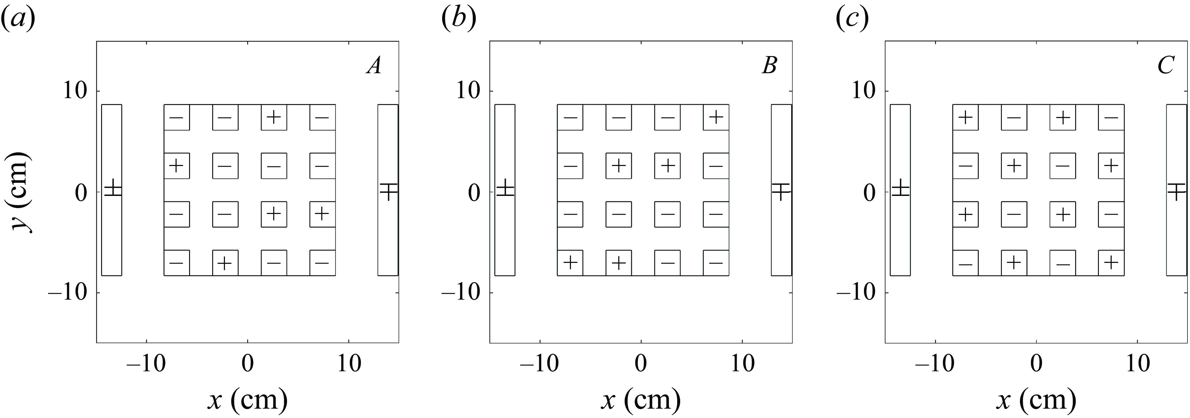
To generate different turbulent flows, the magnets were arranged in three different distributions,
 $A$
,
 $B$
and
 $C$
, as shown in figure 2. We obtain six different forcing configurations by applying the electric current with positive or negative polarity. The forcing scale is the separation between magnets (Kelley & Ouellette Reference Kelley and Ouellette2011), which is approximately 5.1 cm. Distribution
 $A$
consists of
 $11$
magnets with negative and five with positive polarity, arranged in a random pattern (figure 2
a). This asymmetric array causes the applied forcing to induce a preferential positive or negative circulation in the fluid, depending on the direction of the electric current. The second array
 $B$
is a different random arrangement of the magnets (figure 2
b). The resulting forcing generates different realisations of the disordered flow compared with previous cases. Finally, configuration
 $C$
consists of eight magnets with positive polarity and eight with negative polarity arranged alternately, like a chessboard (figure 2
c). This arrangement generates a similar forcing with either sign of the electric current and does not induce a preferential circulation. Additional cases can be defined by varying the magnitude of the electric current or the forcing protocol, as explained in the free-decay (§ 3) and continuously forced (§ 4) experimental sections.
Distributions of 16 magnets (small squares) placed below the square flat sector of the rotating tank. The sign on each magnet is the polarity of the vertical component of its magnetic field. The two rectangles at
 $x=\pm L/2$
indicate the electrodes placed below the topography to generate an electric current. (a) Distribution
 $A$
: random array of 5 positive and 11 negative magnets. (b) Distribution
 $B$
: different random array of 5 positive and 11 negative magnets. (c) Distribution
 $C$
: alternate array of 8 positive and 8 negative magnets. The direction of the electric current defines different forcing configurations.

2.2.3. Flow parameters
Typical velocity and length scales in most of experiments were
 $U\approx 0.5$
cm s−1 and
 $\ell \approx 5$
cm. The Rossby number based on these scales is
 $\textit{Ro}=U/f_0\ell \approx 0.1$
, which is small enough to consider the flow’s bidimensionality. The Reynolds number is
 $\textit{Re}=U\ell /\nu \approx 250$
, so lateral viscous effects are moderate. The Ekman number is
 $E=2\nu /f_0H^2 =2\times 10^{-4}$
, which gives an Ekman time scale
 $T_E=2/f_0E^{1/2}=141$
s or approximately
 $11$
days, which is the decaying time scale associated with bottom friction.
A fundamental factor to mimic oceanic conditions is the topographic
 $\beta$
-effect due to the slopes (Zavala Sansón & van Heijst Reference Zavala Sansón and van Heijst2000). In non-dimensional form, the
 $\beta$
-parameter in the laboratory is
 $\beta '_{\textit{lab}}=\beta _t W/f_0=0.96$
. In a typical mid-latitude ocean basin with Coriolis parameter of
 $10^{-4}$
s
 $^{-1}$
, an abrupt bottom slope
 $10^{-2}$
and mean depth
 $10^3$
m, the topographic parameter is
 $\beta _t \approx 10^{-9}$
m
 $^{-1}$
s
 $^{-1}$
. Thus, considering a horizontal width of the topography of approximately 100 km, the non-dimensional parameter is
 $\beta '_{\textit{oce}} \approx 1$
, which is the same order as the experimental value.
The magnitude of the forcing is measured by the Chandrasekhar number defined as
 $\textit{Ch}=\textit{IBH}/\rho \nu ^2$
, which compares the Lorentz and viscous forces (Duran-Matute et al. Reference Duran-Matute, Trieling and Van Heijst2011). In this definition, it is assumed that the electric current is essentially produced by the potential difference between the electrodes, and not by the much weaker induced currents by Ohm’s law, which are neglected. In most of our experiments,
 $\textit{Ch} \sim O(10^7)$
. High values of
 $\textit{Ch}$
indicate the forcing is intense enough to set the fluid in motion against viscous effects.
2.2.4. Type of experiments
Two different type of experiments were performed:
-
(i) Decaying turbulence. Before an experiment, the tank rotates with the forcing turned off (typically, 40 min) until the water reaches solid-body rotation. Then, the electromagnetic force is applied for two to five days, after which the electric current is disconnected. The fluid presents a disordered state, and the experiment starts. The flow evolves while decaying for 30 days, a long enough time scale for rotational effects to become significant but short enough for viscous processes to remain secondary. In most experiments, the fluid surface was exposed to the ambient air, whose effect was negligible because of the strong density difference between water and air, and because the tank rotates at a moderate angular speed. In some cases, a lid was placed over the free surface to ensure the suppression of such effects, but the ultimate result was an increased Ekman friction. The results are presented in § 3.
-
(ii) Randomly forced turbulence. As in the decaying case, the system is led to solid-body rotation before starting. The experiment begins when the electromagnetic forcing is applied to the motionless fluid (in the rotating system). During the first 20–30 days, the energy injection is balanced with dissipative effects, so the system reaches a state of (quasi) equilibrium. From day 30 to day 55, the polarity of the electrodes is reversed every 5 days to maintain the randomness of the forcing and avoid favouring any particular flow pattern. Finally, on day 60, the forcing is turned off, marking the end of the experiment. The results are presented in § 4.
2.3. Numerical model
The experiments were numerically simulated by solving the shallow-water model (2.3)–(2.5) with a finite differences code (Verzicco et al. Reference Verzicco, Flór, van Heijst and Orlandi1995) that has been tested several times for studying rotating flows over topography (Zavala Sansón & van Heijst Reference Zavala Sansón and van Heijst2002; Zavala Sansón Reference Zavala Sansón2019). The simulations are performed in a square domain with a depth field
 $h(x,y)$
identical to that shown in figure 1. The simulations start with an initial vorticity field
 $\omega (x,y,t=0)$
. By inverting (2.5) with a multigrid method, the initial transport function
 $\psi (x,y,t=0)$
is obtained, and then the temporal evolution of the vorticity (2.3) is calculated using a third-order Runge–Kutta scheme. The nonlinear terms are discretised following an Arakawa scheme. The horizontal velocity components (2.2) are calculated with the transport function derivatives and the depth field. All simulations include a Laplacian viscous term with a suitable viscous coefficient. The boundary conditions are no slip.
Some simulations were devoted to reproducing the decaying experiments using laboratory parameters (table 1), and linear (2.8) or nonlinear (2.9) Ekman friction models. The domain was discretised with a square grid of
 $257 \times 257$
points, so the spatial resolution is
 ${\rm d}x=L/256 \approx 0.08$
cm, with a time step of
 ${\rm d}t=0.025$
s. Another set of simulations was performed using oceanic scales and omitting bottom friction, so the flow decays slowly only due to Laplacian viscosity (with a turbulent coefficient
 $\nu =10$
m
 $^2$
s−1). The aim is to investigate whether the decaying and forced experimental results are reproduced in oceanic-scale systems without the interference of bottom friction. The domain horizontal and vertical scales were
 $L=500$
km and
 $H=1000$
m, respectively (table 1). To solve finer scales than in the laboratory (relative to the domain size), the grid had
 $513 \times 513$
points, so
 ${\rm d}x=L/512 \approx 0.98$
km, with a time step of
 ${\rm d}t=1800$
s. The initial Rossby and Reynolds numbers in decaying simulations were
 $\textit{Ro}\sim 0.1$
and
 $\textit{Re}\sim 1000$
. The duration of all runs was
 $365$
terrestrial days. In forced simulations, we considered a spatially variable and time-dependent function based on harmonic modes (Zavala Sansón Reference Zavala Sansón2022, see § 4).
3. Decaying turbulence
3.1. Experimental results
A total of
 $32$
decaying turbulence experiments were conducted (see § 2.2.4), of which 12 are characterised by (i) the forcing configuration, (ii) the applied electric current, (iii) the forcing time (the number of days that the electric current is applied before turning it off) and (iv) the presence or absence of a solid lid at the upper surface. The other
 $20$
experiments were repetitions aimed at verifying the reproducibility of the results and correcting errors.
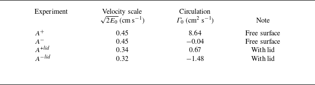
The main results can be illustrated using four experiments listed in table 2, namely,
 $A^{\pm }$
, and
 $A^{\pm }lid$
. The superscript
 $\pm$
indicates the direction of the electric current, which generates different initial vorticity fields (shown in figure 3). Experiments
 $A^{\pm }$
were performed without a top cover, while experiments
 $A^{\pm }lid$
included an upper lid on the surface. To quantify these flows, we consider the total kinetic energy per unit mass defined as
Four representative experiments of decaying turbulence using the distribution of magnets
 $A$
in figure 2(a). The superscripts
 $\pm$
indicate the direction of the electric current
 $I$
(applied over two days). Columns 2 and 3 present the initial velocity scale and circulation. Experiments
 $A^{\pm }$
were performed with the fluid surface uncovered, while experiments
 $A^{\pm }lid$
were conducted with a lid over the surface.

Initial relative vorticity fields (scaled with
 $f_0$
) and velocity fields (arrows) in experiments (a)
 $A^{+}$
, (b)
 $A^{-}$
, (c)
 $A^{+}lid$
and (d)
 $A^{-}lid$
. The inner square indicates the central flat region and the outer region corresponds to the slopes in the periphery. See table 2.

 \begin{equation} E(t)= \frac {1}{2V} \iint h(u^2+v^2)\, \mathrm{d}x\,\mathrm{d}y, \end{equation}
where
 $V=\int h(x,y)\mathrm{d}x\mathrm{d}y$
is the total volume. The velocity scale is
 $\sqrt {2E_0}$
, with
 $E_0$
the initial energy. Experiments
 $A^{\pm }$
in figure 3(a,b) start with a different initial distribution but have the same initial energy and velocity scale. Experiments
 $A^{\pm }lid$
, shown in figure 3(c,d), start with a lower energy and velocity values (table 2). Another useful quantity is the circulation
 \begin{equation} \varGamma (t) = \iint \omega\, \mathrm{d}x\,\mathrm{d}y. \end{equation}
Experiment
 $A^+$
starts with a more positive initial circulation
 $\varGamma _0$
than
 $A^-$
. The same occurs for experiments
 $A^{\pm }lid$
(see table 2).
3.1.1. Flow evolution
Scaled relative vorticity and velocity fields measured in experiment
 $A^{+}$
from day 0 to day 20.

Figure 4 shows the temporal evolution of the horizontal velocity and scaled relative vorticity fields measured in experiment
 $A^{+}$
. At time
 $t=0$
days (immediately after stopping the forcing), the flow appears disorganised, with vortices of various sizes present over both the flat region and the topographic slopes. By
 $t=3$
days, a counter-clockwise circulation over the slopes starts to form, along with an anticyclone accompanied by a smaller cyclone near the centre of the flat region. At
 $t=5$
days, the central anticyclone has intensified, and the cyclonic flow over the slopes is well defined, although it exhibits a wavy pattern. By
 $t=10$
days, the anticyclone has become more circular, occupying most of the flat area, while the cyclonic current continues over the slopes. Finally, at
 $t=15$
and
 $t=20$
days, the cyclonic circulation on the slopes and the central anticyclone persist. At these times, small-scale structures develop, which are attributed to unavoidable additional perturbations in the laboratory (e.g. wind drag, oscillations of the rotating table, convective effects). However, these structures are very small and weak, so they do not interfere with the generation of the topographic current and the central anticyclone. Note that the scale of the velocity vectors and the colour bar for vorticity change over time to highlight the flow characteristics clearly, as the system is in continuous decay.
Now consider the kinetic energy
 $E(t)$
calculated with (3.1). Figure 5(a) shows the
 $E(t)$
curves measured in experiments
 $A^{\pm }$
and
 $A^{\pm }lid$
. For illustrative purposes, the curves start from
 $t\lt -2$
days (when the energy is almost zero); then, the electromagnetic forcing is switched on at
 $t=-2$
days, generating the increase in energy until the forcing is stopped at
 $t=0$
days, when the curves reach a maximum value and define the start of the experiment. For
 $t\gt 0$
, the energy decays over 25 days. The energy curves in experiments
 $A^{\pm }$
(red) are very similar, even though the experiments start from different initial conditions. The kinetic energy decays rapidly at first and more gradually at later times. In experiments
 $A^{\pm }lid$
(blue), the initial energy has a lower value due to the additional friction introduced by the lid. Again, both experiments show the same behaviour during the decay, despite starting from completely different initial conditions.
(a) Evolution of the kinetic energy per unit mass in experiments
 $A^{\pm }$
(solid and dashed red lines), and
 $A^{\pm }lid$
(solid and dashed blue lines). All curves are normalised with the initial energy of experiment
 $A^{+}$
,
 $E_0=0.10$
cm
 $^2$
s−2. A low-pass filter (frequency cutoff of 12.5 s
 $^{-1}$
) was applied to smooth out the noise. The cyan and green solid lines are the theoretical Ekman decay proportional to
 $\exp (-2t/T_E)$
and
 $\exp (-4t/T_E)$
, respectively, with
 $T_E=141$
s. (b) Log–log plots of the curves shown in (a).

The main decay mechanism is bottom friction due to the lower Ekman layer (and the upper layer in the experiments with a lid). This can be verified by comparing the measured energy curves in experiments
 $A^{\pm }$
with the energy decay due to the standard Ekman friction,
 $E(t)/E_0=\exp (-2t/T_E)$
, where
 $T_E$
is the Ekman time scale (see § 2.2.3). For experiments
 $A^{\pm }lid$
, the upper lid causes the friction to double, so the energy decays as
 $\exp (-4t/T_E)$
. Both theoretical curves are included in figure 5(a) (cyan and green) and follow closely the energy decay measured in the experiments. This is further verified in the log–log plots in figure 5(b).
3.1.2. Equilibrium state
To examine the flow state towards which the system evolves, figure 6 presents the time-average vorticity fields
 $\overline {\omega }/f_0$
in experiments
 $A^{\pm }$
(panels a and b) and
 $A^{\pm }lid$
(panels c and d). The average fields are calculated from days
 $5$
to
 $10$
, which is the period in which the main flow features are already generated. All cases clearly show the formation of an anticyclone in the flat region (clockwise arrows and predominantly negative vorticity), and a cyclonic circulation over the slopes. Other less significant features include the meanders in the current over the topographic slopes and the presence of smaller, weaker eddies in the flat region.
Time average of the relative vorticity and velocity fields measured in experiments (a)
 $A^{+}$
, (b)
 $A^{-}$
, (c)
 $A^{+}lid$
, (d)
 $A^{-}lid$
. The average is computed with 63 fields measured between day 5 and 10.

The main average features illustrate the equilibrium state configuration reached by the system regardless of the initial condition (shown in figure 3) and bottom friction magnitude. Indeed, experiments
 $A^{\pm }$
start with a different vorticity distribution and they end up in a similar state (figures 6
a and 6
b). The same occurs in experiments with an upper lid
 $A^{\pm }lid$
(figures 6
c and 6
d). The latter equilibrium states are much weaker because of the enhanced friction.
We can also note detailed differences between the average states in figure 6. The velocity fields suggest that the topographic current is more intense in
 $A^+$
than in
 $A^-$
, while the central vortex is more intense and bigger in
 $A^-$
than in
 $A^+$
. A similar difference is found in experiments
 $A^{\pm }lid$
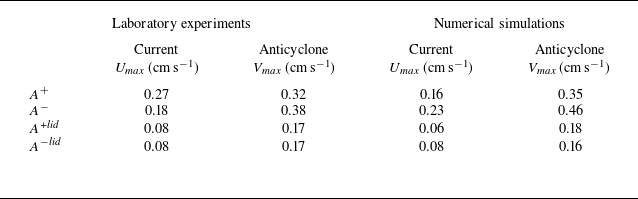
, especially regarding the vortex size. Quantitative estimations of the equilibrium features supporting previous assertions are presented in table 3, where columns 2 and 3 show: (i) the maximum velocity
 $U_{\textit{max}}$
over the slopes to characterise the topographic current, and (ii) the maximum velocity value
 $V_{\textit{max}}$
in the central anticyclone (columns 4 and 5 contain numerically calculated values to be discussed in § 3.2). These differences are related to the circulation of the initial conditions, as shall be further discussed in numerical simulations (§ 3.2.2).
Characteristic velocity of the topographic current over the slopes (
 $U_{\textit{max}}$
) and the central anticyclone (
 $V_{\textit{max}}$
) measured from the equilibrium states shown in figure 6. Columns 2 and 3: laboratory experiments (approximate error
 $\pm 20$
%). Columns 4 and 5: numerical simulations using nonlinear Ekman friction (presented in § 3.2.1).

Summarising the laboratory experiments, the decay of an initially disordered flow in the basin rapidly develops an anticlockwise (cyclonic) current over the topographic slopes. Later, an anticyclone forms in the flat central region. This behaviour was repeated in experiments with different initial conditions and varying magnitudes of frictional effects. The characteristics of the anticyclone and the current over the topography may change in other experiments, but their generation and persistence were observed in all the analysed cases.
3.2. Numerical results
Numerical simulations of decaying flows were conducted using the shallow-water model with topography described in § 2. Two sets of runs were performed. First, simulations of the laboratory experiments using Laplacian viscous effects and Ekman bottom friction. This set of runs demonstrates that the shallow-water dynamics reproduces the main experimental results. Second, idealised simulations of oceanic-scale flows, which include an ad hoc turbulent viscosity coefficient and no bottom friction. These simulations aim to show that the free decay of an oceanic flow evolves towards the equilibrium state found in the experiments. We emphasise that an essential difference from the laboratory-scale simulations is the absence of bottom friction, which is usually negligible at oceanic mesoscales.
3.2.1. Simulations of the laboratory experiments
We simulated numerically experiments
 $A^{\pm }$
and
 $A^{\pm }lid$
. In these four runs, the flow domain and bottom topography are identical to the experimental square box (figure 1). The simulations replicate the relevant parameters in the laboratory shown in table 1. The initial conditions are the interpolated relative vorticity fields shown in figure 3. To simulate experiments
 $A^{\pm }$
, we used Ekman friction that is either linear (2.8) or nonlinear (2.9). The experiments with an upper lid,
 $A^{\pm }lid$
, were simulated by doubling the Ekman friction terms. The evolution time was
 $30$
days (
 $\sim 377$
s).
Velocity fields (arrows) and relative vorticity (surfaces) calculated at different times in the simulation of experiment
 $A^+$
using nonlinear Ekman friction (compare with figure 4).

Figure 7 shows the vorticity and velocity fields at different times in the simulation of experiment
 $A^{+}$
, which can be compared with the panels in figure 4. At time
 $t=0$
days (panel a), the initial field is virtually identical to the experimental one, as it was specifically constructed that way. The simulated flow closely resembles the stages observed in the experiments: the early generation of a cyclonic current over the slopes and the organisation of the central anticyclone. A difference from the laboratory experiment is that the small structures observed at late times are not generated in the simulation, as expected, since they are due to experimental errors, as discussed for figure 4. In this case, nonlinear Ekman friction was used; the simulation with linear friction (not shown) presented marginal differences.
A quantitative comparison of the energy decay in the laboratory experiments and simulations using linear and nonlinear Ekman friction is presented in figure 8. In all cases, there is a good agreement over at least 10 rotating periods (approximately 120 s), with the comparison slightly better when using nonlinear friction. At later times, the simulated energy continues decreasing, whereas a weak noise remains in the laboratory measurements.
Evolution of the kinetic energy calculated in laboratory experiments (blue) and numerical simulations using linear (magenta) and nonlinear (red) Ekman friction: (a)
 $A^{+}$
, (b)
 $A^{-}$
, (c)
 $A^{+}lid$
, (d)
 $A^{-}lid$
. The comparison is slightly better when using nonlinear friction.

Time average of the relative vorticity and velocity fields measured in the numerical simulations of experiments (a)
 $A^{+}$
, (b)
 $A^{-}$
, (c)
 $A^{+}lid$
, (d)
 $A^{-}lid$
. The average is computed with 63 fields measured between day 5 and 10 (compare with figure 6). Nonlinear Ekman friction was used.

The simulations also reproduce the average equilibrium state observed in the laboratory, shown in figure 6. To show it, figure 9 presents the average velocity and vorticity fields of the simulated experiments
 $A^{\pm }$
and
 $A^{\pm }lid$
using nonlinear friction. The averaged fields denote the anticyclone in the basin centre and the cyclonic slope current. Due to the lower friction in the simulations without the lid (panels a, b), the current and the anticyclone are more intense than in cases with a lid (panels c, d). Also, the stronger decay in the latter inhibits the growth of the anticyclone because the flow organisation is halted. Of course, there are qualitative differences with the laboratory measurements, but the overall equilibrium state is similar. Quantitatively, the experimental and numerical velocity values over the slopes and in the central anticyclone can be compared in table 3. These results show that the numerically simulated fluid tends to the mean state observed in the experiments. Thus, we conclude that the dynamics of the physical model is sufficient to generate the observed phenomena in the laboratory.
3.2.2. Effect of the initial circulation
The numerical simulations allow a more thorough examination of the equilibrium state in ocean-scale cases. In what follows, we perform new runs using a square basin with oceanic dimensions, bottom friction is not considered, and lateral friction is parametrised using a weak turbulent viscosity coefficient. Table 1 includes the rest of the oceanic flow parameters. In these simulations, we extend the analyses to better understand the effects of (i) the initial circulation and (ii) the topographic
 $\beta$
-effect.
Consider first the effects of the initial circulation. The laboratory experiments
 $A^{\pm }$
(figure 6
a,b) and the corresponding simulations (figure 9
a,b) showed that the average topographic current is faster and the central anticyclone is weaker in
 $A^{+}$
than in
 $A^{-}$
(see estimations in table 3). The only difference in these experiments is the initial flow configuration (figure 3
a,b) and the initial circulation
 $\varGamma _0$
is more positive in
 $A^+$
(
 $\varGamma ^+_0\gt \varGamma ^-_0$
, see table 2). Therefore, we hypothesise that the more positive the initial circulation, the more intense the topographic current. Equivalently, the more negative the initial circulation, the more intense the central anticyclone. In other words, the strength of the equilibrium state may differ when the initial flow is sufficiently biased to circulate in a pre-established direction (Zavala Sansón Reference Zavala Sansón2025).
(a) Initial relative vorticity and velocity fields in simulation
 $P$
(
 $\varGamma _0=2.2 \times 10^{5}$
m
 $^{2}$
s
 $^{-1}$
). (b) Average vorticity field in run
 $P$
calculated with 150 daily fields from day 200 to 350. Panels (c) and (d) show the same fields for simulation
 $N$
(
 $\varGamma _0=-2.2 \times 10^{5}$
m
 $^{2}$
s
 $^{-1}$
). The initial energy is
 $E_0=0.78 \times 10^{-2}$
m2 s−2 in both runs (or a velocity scale
 $\sqrt {2E_0}\approx 0.12$
m s−1).

Five velocity profiles from ensemble
 $P_i$
(simulations with positive circulation): (a)
 $u_{\!p}$
-profiles along
 $y$
, and (b)
 $v_{\!p}$
-profiles along
 $x$
. (c–d) Same profiles for ensemble
 $N_i$
(simulations with negative circulation). All runs start with the same energy
 $E_0$
and circulation
 $\varGamma _0$
as in figure 10.

Figure 10 presents two oceanic simulations (
 $P$
and
 $N$
) with the same circulation but opposite signs. Both runs lasted
 $365$
days. The initial vorticity fields (panels a and c) consist of a grid of
 $16 \times 16 = 256$
cyclones and anticyclones with a Gaussian profile and having the same amplitude. The field with positive circulation (run
 $P$
) has 160 cyclones and 96 anticyclones arranged randomly (figure 10
a), generating a circulation of
 $2.2 \times 10^{5}$
m
 $^{2}$
s
 $^{-1}$
. The negative configuration (run
 $N$
) has the vortices arranged in the same way as
 $P$
but with opposite signs (figure 10
c); this array generates a circulation of
 $-2.2 \times 10^{5}$
m
 $^{2}$
s
 $^{-1}$
. The two configurations have the same initial energy. Figure 10(b,d) shows the resulting average fields in the two simulations. The equilibrium state is reproduced in both cases: a cyclonic current is established over the topographic slopes, and an anticyclone forms in the central flat region. However, in simulation
 $P$
(panel b), the central anticyclone is much weaker than in simulation
 $N$
(panel d); also, the topographic current over the slopes is much more intense in
 $P$
compared with
 $N$
. These results confirm that the imposed initial circulation influences the characteristics of the equilibrium state.
Since the initial array in simulations
 $P$
and
 $N$
is random, we investigate whether the same equilibrium state is obtained with a different random arrangement having the same energy and circulation. For this purpose, we performed ensembles of simulations with positive and negative circulations,
 $P_i$
and
 $N_i$
, with
 $i=1\ldots 5$
(one of the runs in each group is shown in figure 10). For each member, we calculated the temporal average of the long-term distributions. We found similar equilibrium states as those shown in figure 10(b,d), that is, a strong (weak) topographic current and weak (strong) central anticyclone for ensemble
 $P_i$
(
 $N_i$
) (not shown).
To show quantitative differences between the equilibrium states in the two ensembles, we calculate the long-term temporal-average velocity
 $(\overline {u},\overline {v})$
in each simulation and then take the profiles
 $u_{\!p}(y)$
and
 $v_{\!p}(x)$
across the domain defined as
 \begin{align} \text{$u$-profile along $y$}:& \quad u_{\!p}(y) = \overline {u}(x_0,y), \quad \end{align}
 \begin{align} \text{$v$-profile along $x$}:& \quad v_{\!p}(x) = \overline {v}(x,y_0), \end{align}
where
 $x_0$
and
 $y_0$
are the coordinates of the anticyclone centre in each simulation (which is not necessarily the origin). Figure 11 presents the five profiles obtained from each ensemble. The
 $P_i$
profiles (panels a and b) match between them along the two directions, which indicates that the equilibrium state is practically the same: a strong topographic current and a weak and small anticyclonic structure at the central flat region, as found in figure 10(b). In contrast, the
 $N_i$
profiles (panels c and d) do not coincide exactly, which means that the equilibrium state might present some variations due to the random initial condition. Also, the
 $N_i$
-profiles denote a weaker topographic current and a stronger and bigger central anticyclone, as found in figure 10(d).
3.2.3. Simulations with different topographic
 $\beta$
-effect

To explore the influence of the topographic
 $\beta$
-effect on the equilibrium state, we conducted simulations with oceanic basins having the exact dimensions as in previous cases (
 $L=500$
km and
 $H=1000$
m) but different slopes. All topographies have a width of
 $W=100$
km while the maximum height at the walls
 $D_w$
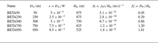
was 50, 250, 500, 750 and 950 m. Thus, cases range from a gentle slope to one with abrupt topography (small to higher topographic
 $\beta _t$
). The simulations are named with the prefix BETA followed by the value of
 $D_w$
(table 4). The initial vorticity field in all cases consists of an arrangement of 128 cyclones and 128 anticyclones resembling a chessboard, which has zero circulation (figure 12
a). Due to the varying slopes, the volume slightly differs in each basin, so the intensity of the vortices in each simulation was adjusted to maintain the same initial energy.
Topographic parameters in simulations with topographies having the same width
 $W=100$
km and different height at the wall
 $D_w$
(second column). In all cases,
 $f_0=10^{-4}$
s
 $^{-1}$
.

To illustrate the results, we consider the equilibrium states calculated in simulations BETA50, 500 and 950. Figure 12(b–d) shows the long-term average velocity and vorticity fields denoting the equilibrium states: the cyclonic current over the slopes and the anticyclonic structure on the flat region of the basin. There are some quantitative differences, such as the more intense topographic current in the simulation with higher
 $\beta _t$
(BETA950, panel d); however, the long-term equilibrium is quite similar regardless of the slope steepness.
(a) Initial vorticity field in the BETA simulations (table 4). Relative vorticity and velocity fields averaged between days 200 and 350 in simulations: (b) BETA50, (c) BETA500, (d) BETA950. In all experiments, the initial energy is
 $E_0=1.4 \times 10^{-2}$
m2 s−2 (or a velocity scale
 $\sqrt {2E_0}\approx 0.17$
m s−1).

The effect of
 $\beta _t$
is reflected in the phase speed of the topographic waves generated over the slopes and propagating towards the local ‘west’; i.e. with shallow water to the right. Eventually, the waves are organised as the cyclonic topographic current or ‘zonal’ flow (see § 9.1.1 of Vallis Reference Vallis2017). To visualise the waves, we built Hövmoller diagrams of the average cross-slope vorticity field over 300 km along one of the lateral walls. Figure 13(a) presents the Hövmoller diagram for run BETA500. The waves are unclear at the initial stages (
 $t\lt 50$
days) because turbulent motions dominate. For
 $t\gt 50$
days, the waves are clearly identified by the vorticity stripes with negative slope, as shown in the zoom between days 50 and 150 in figure 13(b). In the long term, the waves are damped and become less visible. Using similar diagrams, we also found the signal of topographic waves in simulations BETA50 and BETA250. However, the waves were hardly visible in BETA750 and BETA950, because
 $\beta _t$
is so high that wavy motions are quickly incorporated into the cyclonic current.
To show that the oscillations shown in figure 13(b) are topographic waves, consider the dispersion relation for a barotropic wave travelling in the local western direction as
 $\sigma =-\beta _t k/(k^2+R_d^{-2})$
, where
 $\sigma$
is the frequency,
 $k$
is the wavenumber along the slope and
 $R_d=\sqrt {gH_m}/f_0 \approx 852$
km is the deformation radius with
 $g$
the gravity. Assuming
 $k\approx 2\pi /W$
, then
 $k^2\gg R_d^{-2}$
, so the phase speed can be estimated as
 \begin{equation} c \equiv \frac {\sigma }{k} \approx -\frac {\beta _t}{k^2}. \end{equation}
For simulation BETA500 we find
 $c\approx -15$
km d−1. The speed of the signals shown in figure 13(b) is given by the slope
 $\approx -17$
km d−1, which is very close to the calculated value. We verified that the phase speed of the waves detected in runs BETA50 and BETA250 also obey (3.5) (in these cases,
 $c\approx 5$
km d−1 and 12 km d−1, respectively). The simulations confirm the presence of topographic waves, which were not detected in the experiments, probably because experimental errors mask these oscillations, and damping effects are much more intense.
(a) Hövmoller diagram for the average cross-slope vorticity along 300 km in simulation BETA500. (b) Zoom between 50 and 100 days. The slope of the vorticity signal is
 $-17$
km d−1 (the theoretical value is
 $\approx -15$
km d−1, see text).

4. Randomly forced turbulence
Now we examine the case of a continuously forced fluid in the same idealised basin. We aim to demonstrate that the long-term average fields are characterised by the cyclonic current over the slopes and the central anticyclone, even in the presence of the disordering action of the continuously applied forcing. We present experimental results first, followed by numerical simulations using oceanic scales.
4.1. Experimental results
The experiments with a continuous forcing were described in § 2.2.4. We conducted 12 experiments, of which six were repetitions. The forcing in most experiments was applied using the magnet distribution
 $C$
(a chess-like distribution), shown in figure 2(c). To illustrate the main results and their reproducibility, measurements taken from a particular experiment
 $C^+_1$
and its repetition
 $C^+_2$
are presented in this section.
4.1.1. Flow evolution
Scaled relative vorticity (surfaces) and velocity fields (arrows) measured in the continuously forced experiment
 $C^+_1$
from day 30 to day 55. At these times, the flow has reached a statistically quasi-steady turbulent state.

The fluid starts from rest, and the forcing is applied for 60 days. Then, between days 30 and 60, the system reaches a statistically stationary state where the energy injection is nearly balanced with viscous dissipation. Figure 14 presents six snapshots of the relative vorticity in experiment
 $C^+_1$
to show the unsteady evolution once the flow has reached a turbulent state. These fields show the unsteadiness and disordered behaviour of the flow within the statistically stationary stage. The flat central region seems to contain larger structures than the periphery. However, closely inspecting the velocity field over the topographic slopes (along the lateral walls) reveals a predominantly cyclonic flow with shallow water to the right. Similar results are obtained in the twin experiment
 $C^+_2$
(not shown). This behaviour has been observed in previous
 $f$
and
 $\beta$
-plane simulations in a similar basin (Zavala Sansón Reference Zavala Sansón2022, Reference Zavala Sansón2025).
Evolution of the kinetic energy per unit mass in experiments
 $C^+_1$
and
 $C^+_2$
(red and green lines, respectively). The curves are normalised with the mean energy between days 30 and 60,
 $E_m=4.2\times 10^{-6}$
m2 s−2. A low-pass filter (frequency cutoff of 12.5 s
 $^{-1}$
) was applied to smooth out the noise. The vertical grey lines indicate the 5-day period at which the Lorentz forcing was reversed to avoid favouring any circulation.

Figure 15 shows the evolution of the total kinetic energy for both realisations,
 $C^+_1$
and
 $C^+_2$
. At the beginning of the experiments, the energy continuously increases until reaching its first peak on day 6, after which it decreases, only to rise again and reach a quasi-stable energy value for the rest of the experiments. The vertical grey lines between days 30 and 60 indicate the approximate time the Lorentz forcing was reversed to maintain the randomness and avoid favouring a particular flow pattern. Finally, on day 60, the forcing is turned off, marking the end of the experiment. Both curves present similar oscillations despite the unavoidable subtle differences in the execution of the two realisations. The energy curves demonstrate the reproducibility of the experiments and that the continuously forced system reaches a statistically quasi-stationary turbulent state between days 30 (or even less) and 60.
4.1.2. Equilibrium state
Time average of the relative vorticity and velocity fields measured in experiments (a)
 $C^+_1$
, (b)
 $C^+_2$
. The time average is computed with 376 fields measured between day 30 and 60.

Now we examine the mean state reached by the flow despite the presence of the continuous forcing. Figure 16 shows the averaged velocity and vorticity fields between days
 $30$
and
 $60$
in the twin experiments. In both realisations, the cyclonic flow is neatly observed over the slopes, while a robust anticyclone is formed at the flat region. Again, the similarity between the fields demonstrates the reproducibility of the experiments and the consistency of the results. The most remarkable feature is that this equilibrium configuration is similar to the decaying case. Therefore, we conclude that the average formation of a central anticyclone in a basin is a robust phenomenon even in the presence of the forcing.
4.2. Numerical results
We conducted simulations of forced turbulence to verify the presence of the equilibrium state in the shallow-water dynamics using oceanic scales and in the absence of bottom friction. These runs use the same domain and topography employed in the free-decay oceanic simulations
 $P$
and
 $N$
presented in § 3.2.2. The duration of the simulations, the turbulent viscosity coefficient and the spatial and temporal resolution are also the same as in the decaying oceanic cases.
In these runs, a spatially and temporally variable forcing term is included in the vorticity (2.3). The spatial dependence of the forcing is given by a sum of six harmonic modes with different wavelengths
 $(k_i,l_i)$
(
 $i=1\ldots 6$
), and the time dependence is contained in the corresponding phases that change randomly every time step, so the net forcing direction is also random (see details in Zavala Sansón Reference Zavala Sansón2022). This forcing is based on a first-order Markov process with a three-day decorrelation time, so it slowly evolves in time (Lilly Reference Lilly1969). All the forcing modes have a similar wavenumber magnitude (
 $\kappa _f \approx 1.5 \times 10^{-4}$
m
 $^{-1}$
) that sets the forcing scale at
 $\ell _f\approx 2\pi /\kappa _f \approx 42$
km or
 $\ell _f\approx L/12$
. This value is comparable to the mid-latitude first Rossby deformation radius, which can be considered the energy injection scale in geostrophic turbulence (Salmon Reference Salmon1998). Note that
 $\ell _f\approx 0.4W$
, which is smaller than the forcing scale used in the experiments. The amplitude of the forcing function is chosen so that the mean total energy is similar to the initial energy of the decaying simulations
 $P$
and
 $N$
(shown in figure 10).
4.2.1. Equilibrium state in forced simulations
Time average of the relative vorticity and velocity fields measured in simulations (a)
 $F_1$
, (b)
 $F_2$
. The time average is computed with 265 daily fields between days 100 and 365. Both fields have a similar mean energy,
 $E_m=0.72 \times 10^{-2}$
m
 $^2$
s−2, but are generated with a different random forcing.

Time evolution of (a) the kinetic energy per unit mass (red curve for the total value, purple over the slopes and green over the central flat region), and (b) regional circulations (same colour code) in simulation
 $F_1$
. All energy curves are normalised with the mean energy
 $E_m$
calculated between days 100 and 365. Panels (c) and (d) show the same quantities for simulation
 $F_2$
.

Here, we present the results from two simulations,
 $F_1$
and
 $F_2$
, where the fluid is maintained in motion by forcing terms having the same amplitude but different random protocols (defined by different random phases of the forcing harmonic modes), so they develop the same mean energy once they reach statistical equilibrium. The simulated time evolution is similar to that observed in the experiment shown in figure 14: the flow is set in motion from rest, and some time later it reaches a statistically stationary turbulent state (not shown). In what follows, we will focus on the average fields of the turbulent stage.
Figure 17 presents the time-average vorticity and velocity fields in simulations
 $F_1$
and
 $F_2$
. Again, despite the continuous action of the random forcing, a preferred state can be observed in all fields. The velocity vectors indicate that, on average, a cyclonic current forms over the slopes near the boundaries, while an anticyclonic flow develops in the basin’s centre. As expected, the averaged vorticity fields present small-scale variability due to the continuous forcing. However, it is still evident that the vorticity is predominantly negative in the centre of the basin with the formation of the cyclonic topographic current with shallow water to its right.
The evolution of the total kinetic energy in simulation
 $F_1$
, normalised by the mean energy at equilibrium (
 $E_m$
), is presented in figure 18(a) (red curve). The energy measured over the slopes and the flat region is also shown (purple and green curves, respectively). Throughout the simulation, approximately 50 %–60 % of the energy is concentrated over the slopes, while the remaining portion is in the central flat area. We also calculated the circulation in the two regions. In figure 18(b), it can be seen that, during the first days, there is no clear preference to concentrate the circulation in any region. Once the statistically steady state is reached, a clear distinction emerges: circulation is positive over the slopes and negative in the central region. This result is consistent with the averaged fields previously shown. Figure 18(c,d) presents the same curves for simulation
 $F_2$
. These plots show that a similar evolution of the energy curves and regional circulations occurs when using a different seed for the random forcing.
5. Discussion and conclusions
We presented laboratory experiments and numerical simulations (based on a shallow-water model) of one-layer, quasi-2-D turbulence in the interior of an idealised closed basin in a rotating system with a flat interior and surrounded by steep slopes. The results were focused on two different problems: (i) the decay of an initially random flow (§ 3), and (ii) the evolution of a continuously forced flow (§ 4). An important feature of the basin is that the topography has abrupt slopes that impose a strong topographic
 $\beta$
-effect that surpasses the planetary
 $\beta$
-effect by at least one order of magnitude. Thus, the shallow-water dynamics is preferable to the quasi-geostrophic limit, which is restricted to less steep topographic variations.
5.1. Decaying and forced experiments
In the free-decay experiments, the initial flow is randomly generated by applying a horizontal electromagnetic Lorentz force (e.g. Sommeria Reference Sommeria1986; Bondarenko et al. Reference Bondarenko, Gak and Gak2002). In all cases, a persistent current is formed around the basin over the topographic slopes with shallow water to the right (with the Coriolis parameter defined positive). The topographic current is generated during the first few rotation periods or ’days’. Essentially, the topographic
 $\beta$
-effect induces the propagation of all perturbations along the local ‘west’ direction (along slope with shallow water to the right). As a result, the energy is channelled in the observed cyclonic current. At approximately 10 days, the flow at the flat region of the basin is organised into a single anticyclonic structure that persists during the rest of the experiments (up to 25 days). Given the relatively short length scales of the experimental basin (figure 1), the flow rapidly decays, mainly due to bottom friction effects. Nevertheless, since the formation of the peripheral current and the central anticyclone occur over sufficiently long times (longer than the system’s rotation period), it is concluded that they are not a consequence of viscous effects, but rather a result of the nonlinear flow evolution.
We performed numerical simulations with a shallow-water model to investigate the flow dynamics. First, the experiments were simulated using the same laboratory parameters, and the numerically calculated fields reproduced the equilibrium state to good accuracy. These simulations confirmed that the flow dynamics in the experiments is quasi-two-dimensional. Second, additional simulations based on the same model but using an oceanic-scale basin on the
 $f$
-plane were carried out. The main difference from the simulated experiments was the absence of Ekman friction, since upper-ocean flows barely experience bottom dissipation. We aimed to draw an explicit parallel between the laboratory and geophysical problems. Overall, these runs demonstrated that the same equilibrium is reached. The experimental and numerical results showed that the initial condition and the value of the topographic
 $\beta$
parameter might influence the characteristics but not the configuration of the long-term average state.
The randomly forced experiments started with the fluid at rest, and then were set in motion by systematically applying the electromagnetic forcing. The flow reached a statistically quasi-stationary state between days 20 and 30 and continued evolving randomly during the rest of the experiments (which lasted up to 60 days). The instantaneous flow fields were clearly unsteady and disordered. However, the average vorticity and velocity fields showed the presence of the peripheral mean current over the slopes, and the central region exhibited a mean anticyclonic vortex. This remarkable result suggests that the average flow in a flat basin with a steep sloping bottom adjacent to the sidewalls tends to the equilibrium configuration, even when the forcing is entirely random in time and space. Numerical simulations confirmed that the mean equilibrium configuration arises again. The forced simulations were performed using oceanic scales, do not include bottom friction and the relative forcing scale (in comparison with the domain size) is smaller than in the experiments.
5.2. On the origin of the equilibrium state
The formation of the topographic current is in agreement with maximum entropy or minimum enstrophy classical quasi-geostrophic theories (Bretherton & Haidvogel Reference Bretherton and Haidvogel1976; Salmon et al. Reference Salmon, Holloway and Hendershott1976), and also with statistical equilibrium states in topostrophic turbulence (Holloway Reference Holloway1992, Reference Holloway2008). However, it must be remembered that flows in the present experiments are far from equilibrium when decaying or continuously forced. The out-of-equilibrium condition, especially in the randomly forced case, suggests that non-equilibrium theories may be formulated for the shallow-water dynamics. This study is not devoted to developing such a theory, but to demonstrating that the system tends to some identifiable equilibrium, opening a doorway to explore theoretical formulations.
The formation of the central anticyclone has been discussed for a two-layer system, proposing that it is related to stability properties of anticyclones and instability of cyclones (LaCasce et al. Reference LaCasce, Palóczy and Trodahl2024). The turbulent nature of our experiments does not allow us to confirm such a mechanism. Another explanation is related to the downslope topographic advection of anticyclonic vorticity towards the basin’s centre (due to the local topographic
 $\beta$
-effect). A similar mechanism would remove cyclonic vorticity upslope and away from the basin’s centre (Solodoch et al. Reference Solodoch, Stewart and McWilliams2021). We tried to measure the vorticity flux between the continental slopes and the central region with no conclusive results.
5.3. Is there a unique equilibrium state?
The present results do not imply that the equilibrium configuration is unique. For decaying turbulence, the specific features of the equilibrium state suggest a dependence on the initial energy and circulation. When the initial circulation is positive, the topographic current at equilibrium is more intense and the central anticyclone weaker (see the subtle differences in experiments
 $A^{\pm }$
in figure 6(a,b), and the more evident differences in simulations
 $P,N$
with oceanic scales in figure 10). An equivalent result was found in the statistical mechanics theory by Chavanis et al. (Reference Chavanis, Naso and Dubrulle2010), who discussed equilibrium in a square basin for inviscid quasi-geostrophic flows, and found that the central vortex sign depends on the flow energy. This property suggests similar formulations could be designed for decaying or forced flows in the shallow-water dynamics. It is also worth mentioning the statistical mechanics theory by Renaud, Venaille & Bouchet (Reference Renaud, Venaille and Bouchet2016), which requires a non-zero circulation flow or a non-zero bottom topography to sustain a non-trivial shallow-water equilibrium state.
In forced turbulence, the equilibrium might be affected if the average forcing over the whole basin induces a dominant circulation. This preferential forcing may lead to the formation of weaker anticyclones or even the generation of cyclones. According to this mechanism, the frequent formation of the so-called Campeche cyclone in the south-west of the Gulf of Mexico might be due to the persistent positive wind curl that is present most of the year (Zavala-Hidalgo et al. Reference Zavala-Hidalgo, Romero-Centeno, Mateos-Jasso, Morey and Martínez-López2014). This generation mechanism was addressed using equivalent-barotropic simulations in Zavala Sansón (Reference Zavala Sansón2019).
Another factor that might influence the equilibrium characteristics is the shape of the basin. We chose a rotating system that combines two problems that previous works have studied separately: the self-organisation of a 2-D flow over a flat bottom and the flow–topography correlation over non-flat regions. When the central area is no longer flat but, e.g. Gaussian or parabolic, preliminary simulations in a parallel study (Suaza et al., in prep.) suggest that a more ‘round’ central region might lead to the formation of cyclones, or at least the inhibition of anticyclones. Finding a different equilibrium in higher Reynolds number flows is also possible. Definitive results will be published elsewhere.
5.4. Remarks about the experiments
Obtaining reliable and reproducible experimental results is not a trivial task. One of the main problems is that any slight perturbation triggers the topographic current, so it becomes very hard to start an experiment from absolute rest (in the rotating system). Such perturbations may arise from the contact of the free surface with ambient air or from tiny irregularities of the rotating device. Therefore, the experiments must be performed in a properly isolated environment using a high-precision rotating table.
Another experimental difficulty is that the flow motions are very weak (of the order of 0.1 cm s−1), mainly because the electromagnetic forcing is relatively weak and, in addition, viscous effects are more intense. This limitation implies that the PIV measurements have to be performed carefully. To generate larger velocities with a higher Reynolds number, the experiment could be designed in a larger rotating tank with a deeper fluid layer (to reduce bottom friction) and with a stronger forcing imposed. These are feasible solutions and can be recommended for future studies. However, there would be additional experimental challenges. For instance, the electromagnetic forcing is weaker for deeper fluids, since the vertical magnetic field of the underlying magnets decays very rapidly. Overcoming this problem implies that even stronger magnets, more intense electric currents and conductive fluids should be used.
A common source of undesired motions is the formation of small bubbles generated by electrolysis at the electrodes, which, in the long term, escape to the surface and contaminate the measurements near the walls. We used graphite electrodes because this material is very affordable, easy to obtain and manageable to implement. The problem with bubbles is minor in the free-decay experiments because they do not appear during the short period when the forcing is applied. In the continuously forced experiments, the bubbles might become a problem near the boundaries after 60 periods. In any case, it may be better to use a different material, such as titanium electrodes, and to isolate them more efficiently (Duran-Matute et al. Reference Duran-Matute, Trieling and Van Heijst2011) to minimise this problem further.
Acknowledgements
F.J.R.M. gratefully acknowledges financial support from Consejo Nacional de Humanidades, Ciencias y Tecnologías (Conahcyt), México.
Funding
This work was supported by the Consejo Nacional de Humanidades, Ciencias y Tecnologías (CONAHCYT), México, under Grant No. 1197569.
Declaration of interests
The authors report no conflicts of interest.