


1 Introduction
The vortex shedding behind unconfined bluff bodies has been extensively researched since the independent discovery of the phenomenon in the early 1900s by Henri Bénard and Theodor von Kármán; Wesfried (Reference Wesfreid2006) provides a historical account. Reviews of such flows have been compiled by Roshko (Reference Roshko1954, Reference Roshko1993) and Williamson (Reference Williamson1997).
Research concerning vortex shedding behind confined bluff bodies is, however, more limited, see e.g. Rehimi et al. (Reference Rehimi, Aloui, Nasrallah, Doubliez and Legrand2008). Confined bluff bodies are commonly found in industrial applications (e.g. tube heat exchangers) and are the basic element of vortex flowmeters (VFMs). Vortex flowmeters typically use ‘shedders’ which have a relatively high blockage ratio; this is defined as the ratio of shedder maximum thickness to pipe diameter (
 $d/D$
). Values of approximately 0.3 are common, see Venugopal, Agrawal & Prabhu (Reference Venugopal, Agrawal and Prabhu2011b
). For practical reasons, VFMs typically operate in the high Reynolds number regime (
 $10^{3}\lesssim Re_{d}\lesssim 10^{5}$
), wherein the dimensionless shedding frequency is approximately constant, e.g. Roshko (Reference Roshko1954). Splitter plates (tails) are also commonly utilised to suppress low frequency ‘noise’ in the shedding spectra, as discussed by Miau et al. (Reference Miau, Yang, Chou and Lee1993a
,Reference Miau, Yang, Chou and Lee
b
).
Richter & Naudascher (Reference Richter and Naudascher1976) present an investigation of the effects of channel confinement on shedding frequency of circular cylinders for
 $1/6\leqslant d/D\leqslant 1/2$
. The dimensionless frequency depends on the shedder cross-section, with sharper geometries yielding higher frequencies. They demonstrate that the dimensionless frequency undergoes a rapid increase (in some cases more than doubling) as a result of transition on the shedding body. This occurs beyond a critical Reynolds number (
 $Re_{d}\gtrsim 10^{5}$
). Transition occurs at higher
 $Re_{d}$
for lower blockage ratios. At supercritical Reynolds numbers, the dimensionless frequency appears to slowly increase with Reynolds number.
A recent work by Ford, Winroth & Alfredsson (Reference Ford, Winroth and Alfredsson2018) examined the influences of shedder geometry on vortex shedding of confined bluff bodies. The study highlighted a bi-modal behaviour: mode-I was associated with shedding of the primary vortex, i.e. classical vortex shedding. It possessed a broadly constant dimensionless frequency (
 $St_{d}$
). Mode-II was attributed to a pipe-wall boundary-layer separation, caused by the presence of the shedder (i.e. a consequence of confinement). Mode-II initiated at a higher dimensionless frequency than mode-I and
 $St_{d}$
always decreased as Reynolds/Mach number increased. By way of example, figure 1 shows the mode-I and mode-II dimensionless frequencies (Strouhal numbers) based on the shedder characteristic dimension (
 $d$
) for various tested geometries.
Mode-I (a) and mode-II (b) dimensionless frequencies as a function of Reynolds number for various geometries;
 $h$
indicates the shedder-step height, and
 $l$
the splitter-plate length.

Time–frequency analysis reveals that modes-I and II temporally coexist. For certain geometries and Reynolds numbers, modes-I and II interact and in some cases mode-I locks-on to the mode-II frequency. Ford et al. (Reference Ford, Winroth and Alfredsson2018) hypothesised that this can only occur if the length scales of mode-I and mode-II are in sufficient proportion (i.e. the length scale of mode-II must be large enough) and the frequency ratio is close to an integer value. A detailed description and theoretical model is presented by Ford et al. (Reference Ford, Winroth and Alfredsson2018).
The emergence of mode-II is thought to be a peculiar consequence of the confinement. Hence mode interaction uniquely affects confined vortex shedding. In this study the effects of mode interaction are addressed in the context of flow topology. Several flow visualisation experiments are presented to elucidate the topology of mode-I and how it is altered by mode interaction.
A number of relevant visualisation studies have been published. Anderson & Szewczyk (Reference Anderson and Szewczyk1997), for example, present a study of the primary shedding of cylinders with various splitter-plate lengths (
 $0\leqslant l/d\leqslant 2$
). The body was in low confinement (
 $d/D\approx 0.06$
) and visualisation was presented at
 $Re_{d}=5700$
. The authors report significant influence of the tail. Tail lengths exceeding 0.75
 $d$
cause an elongation of the shear layer, although no fundamental change to the flow topology is observed in the images presented. However, the splitter plates were thin, and therefore the tail length (
 $l$
) remained short in comparison to the primary vortex scale (
 $\unicode[STIX]{x1D705}$
):
 $l/\unicode[STIX]{x1D705}\lesssim 2$
.
Bearman (Reference Bearman1965) presents a flow visualisation study of a low-confinement bluff body (
 $d/D=0.03$
) at Reynolds numbers relevant to the present study (
 $10^{4}\lesssim Re_{d}\lesssim 10^{5}$
). The study shows an image obtained with a long splitter plate (
 $l/d=4$
), identifying a spanwise uniform reattachment line. However, only approximately 30 % of the model span is presented in the image. The authors report that similar reattachment lines were seen for tails with lengths greater than
 $2.9d$
.
Another flow visualisation study was made by Ruderich & Fernholz (Reference Ruderich and Fernholz1986) for flat-nosed bodies with very long splitter plates (
 $l/d\approx 30$
) at
 $Re_{d}=O(10^{4})$
. The study was conducted in a square section wind tunnel (
 $d/D\leqslant 0.1$
) and a highly three-dimensional (3-D) flow field was observed via surface oil film and smoke injection. In stark contrast to Bearman (Reference Bearman1965), the data demonstrate that the reattachment line is not spanwise uniform. The images shown by Ruderich & Fernholz (Reference Ruderich and Fernholz1986) bear a striking resemblance to figure 9 in § 3.2 of the present work.
The present study augments the data of Ford et al. (Reference Ford, Winroth and Alfredsson2018) with new, Reynolds number matched data. The experimental set-ups are briefly described in § 2. The wake topology and the effect of splitter-plate length are discussed in § 3. The effect of mode interaction on the topology of mode-I is discussed in § 4. The scaling of mode-II is considered in § 5. A summary is provided in § 6
2 Experimental set-up
Two Reynolds matched flow facilities were used in this study. These are referred to at the CICERO and NT rigs. CICERO is a small-scale (
 $D=40~\text{mm}$
) moderate Mach number rig. The NT rig is a large-scale (
 $D=194~\text{mm}$
) incompressible facility. A summary of the Reynolds/Mach numbers covered by the facilities is provided by figure 2. The NT experiments were designed to cover the same Reynolds number range as CICERO. However, the NT-2011 tunnel was unable to draw enough flow to exceed
 $Re_{d}\approx 6\times 10^{4}$
.
Reynolds (
 $Re_{d}$
) and Mach number (
 $M_{b}$
) space covered by the two experimental facilities.

2.1 The CICERO rig
A schematic of the CICERO rig is show in figure 3. Two screw compressors (C) pressurise a large tank (T) to 530 kPa. The supply pipe bifurcates into the main and bypass branches, the former feeding the working section. The flow rate through the branches is controlled via ball valves (
 $\text{V}_{m}$
and
 $\text{V}_{b}$
, respectively). The mass flow through the main branch is metered with an ABB FMT500-IG hot-film type flowmeter (A). The accuracy of the mass-flow measurement is better than
 $\pm 0.7\,\%$
of the set point. The flow passes through an 18 kW electric heater (H) before heading to either of two test sites, selected using two butterfly valves (
 $\text{V}_{ba}$
and
 $\text{V}_{bb}$
). After the butterfly valve a conic contraction (n) reduces the pipe diameter (
 $D$
) from 80 mm to 40 mm. The test section (M) is connected to the contraction using a
 $40D$
long straight pipe. A
 $9.5D$
straight pipe is mounted downstream of the working section.
Schematic of the CICERO rig. A, reference flowmeter, C, compressor, H, heater, M, test section, n, contraction, T, pressure tank,
 $\text{V}_{x}$
indicates various valves,
 $D$
indicates pipe inner diameter.

The stagnation pressure was measured using a tap on the leading edge of shedder and the static pressure was recorded
 $0.8D$
upstream of the shedder. The pressures were measured using Motorola MPX5100 differential pressure sensors, which have a pressure range up to 100 kPa and a quoted accuracy of
 $\pm 2.5\,\%$
of full-scale output. Temperature was measured
 $1.5D$
upstream of the test section using a K-type thermocouple and Fluke 51-II thermocouple reader, with an accuracy better than
 $\pm 0.3~\text{K}$
. The vortex shedding frequency was detected using a pair of Norrsonic type 1245 microphones at the pipe wall
 $0.4D$
downstream of the shedder step.
The bulk axial velocity (
 $U_{b}$
) was determined using the measured mass flow (
 ${\dot{m}}$
) and the density (
 $\unicode[STIX]{x1D70C}$
, determined from the measured temperature and static pressure) as
 $$\begin{eqnarray}\displaystyle U_{b}={\displaystyle \frac{4{\dot{m}}}{\unicode[STIX]{x03C0}\unicode[STIX]{x1D70C}D^{2}}}. & & \displaystyle\end{eqnarray}$$
The upstream turbulence intensity, estimated from hot-wire measurements made during commissioning of the rig, was approximately 2.5 to 3.5 % (depending on the Reynolds number). The 40
 $D$
inlet length ensures that the pipe flow is close to fully developed prior to the working section.
In a series of preliminary experiments, the effects of upstream pipe length and downstream pipe length were investigated. Installation effects may adversely influence the calibration of vortex meters. Venugopal, Agrawal & Prabhu (Reference Venugopal, Agrawal and Prabhu2011a
) recommend the inclusion of 20
 $D$
upstream and 5
 $D$
downstream, although 30–40
 $D$
is recommended when complex bend patterns exist in the pipeline (wherein large-scale turbulent structures are likely present).
Previous experiments (Ford, Winroth & Alfredsson Reference Ford, Winroth and Alfredsson2016) have demonstrated the existence of a mode-I/II behaviour with a 22
 $D$
inlet length (although with a slightly different shedder design). Commissioning tests established that the shedding behaviour described herein was insensitive to the length of pipe upstream and downstream of the working section. Experiments were run with the 40
 $D$
straight inlet pipe removed, as well as with various downstream lengths: 1.25, 9.5 and 21
 $D$
. No impact was observed on the principal shedding mode, or the secondary mode. This insensitivity to inlet length is important, because when at the NT rig scale it is impractical to include an inlet section of 40
 $D$
(which would be approximately 8 m).
2.2 The NT rig
The NT rig was set up in the NT-2011 wind tunnel of the KTH Fluid Physics Laboratory. The wind tunnel has a
 $0.4\times 0.5~\text{m}^{2}$
cross-section and is 1.5 m long. The open-loop wind tunnel takes air from the laboratory which is conditioned by a honeycomb and a set of three screens prior to a 9 : 1 contraction. Flow is drawn through the rig by a variable-speed axial fan mounted in the diffuser downstream of the test section. A pipe rig was built wholly within the working section, a schematic is shown in figure 4.
Front view and meridional cross-section of NT rig.

The pipe rig had an inner diameter (
 $D$
) of 194 mm and was mounted horizontally in the working section of the wind tunnel; it was levelled to ensure zero incidence to the oncoming flow. The regions between the pipe and the tunnel walls were filled with foam. The pipe had a small, smooth contraction at the inlet end to prevent any large-scale inlet separation.
The mean (bulk) axial velocity (
 $U_{b}$
) was obtained by a differential reading of the upstream stagnation pressure (
 $p_{0}$
) and the static pressure
 $p_{w}$
measured at the pipe wall using a Furness FCO12-model 3 manometer. The bulk velocity was then defined from the measured inlet dynamic pressure (
 $q=p_{0}-p_{w}$
) as
 $$\begin{eqnarray}\displaystyle U_{b}=\left(\frac{2q}{\unicode[STIX]{x1D70C}}\right)^{1/2}, & & \displaystyle\end{eqnarray}$$
where the air density was computed from ambient properties and assumed to be constant.
Vortex shedding was detected using the same transducers as in the CICERO rig (NorrSonic type 1245 microphones) mounted opposite to each other on the pipe wall and positioned 0.4
 $D$
downstream of the shedder step, consistent with the CICERO rig experiments. As with the CICERO data, the microphone signals were recorded separately but were subtracted prior to data reduction, to create a single pseudo-differential signal. This amplified the frequencies that had anti-phase behaviour and diminished in-phase elements.
The uncertainty of the measured dynamic pressure was
 $\pm 0.5\,\%$
of full-scale output, the manometer is equipped with a 10 % or 100 % range option, so the uncertainty in a dynamic pressure less than 200 Pa was
 $\pm 1~\text{Pa}$
and above 200 Pa was
 $\pm 10~\text{Pa}$
. Resultantly, the uncertainty in Reynolds number is approximately
 $\pm 7\,\%$
to 0.2 %, with the highest values being at the lowest Reynolds numbers and quickly reducing. The temperature was recorded with the same equipment as in the CICERO experiment. Ambient pressure was measured within 10 Pa. The resulting uncertainty in fluid density was around 0.1 %. The viscosity (
 $\unicode[STIX]{x1D707}$
) was computed from temperature using Sutherland’s formula (Sutherland Reference Sutherland1893).
Data were acquired over 1 s at 20 kHz using a National Instruments NI-PCI 6250 A/D converter. Signals have been ensemble averaged, using 20 independent ‘observations’ (20 s of data in total). Extracting frequency information from the microphone signals was achieved using a fast Fourier transform (FFT) and an automatic peak-finding algorithm. Typically peak frequency can be ascertained to within
 $\pm 1~\text{Hz}$
. Tests were executed multiple times and all data were repeatable to within approximately
 $St_{d}\pm 0.01$
.
2.3 Shedder geometry and dimensions
The shedders used in both rigs were non-dimensionally identical. Figure 5 shows the defining dimensions of the geometry:
 $d$
is the maximum shedder thickness,
 $l$
is the length of the tail and
 $h$
is the step height between the shedder body and the tail. Several tail lengths and thicknesses have been considered. Tails have been classed as short or long based on the length relative to the shedder thickness, as indicated in the figure. The forebody is a
 $90^{\circ }$
wedge, with a leading edge radius of
 $0.08d$
. The shedder is mounted in a circular pipe, hence the dimensionless span of the shedder is unity.
A summary of the tested conditions and geometries of the two experimental rigs is provided in table 1. In the CICERO rig five different step heights
 $h$
(
 $0.28<h/d<0.50$
) were used whereas in the NT rig
 $h/d$
was fixed to 0.39.
Shedder geometry highlighting critical dimensions. Flow from left to right as viewed.

A comparison of experimental rig conditions: CICERO and NT rigs.

2.4 Definitions
Throughout this paper, the frequency (
 $f$
) is regularly converted to Strouhal number (
 $St$
), the dimensionless equivalent, viz,
 $$\begin{eqnarray}\displaystyle St_{d}=\frac{fd}{U_{b}}, & & \displaystyle\end{eqnarray}$$
where
 $d$
is the shedder thickness. The bulk velocity (
 $U_{b}$
) is assumed to be the characteristic velocity, as it is for the Reynolds number and bulk Mach number (
 $M_{b}$
),
 $$\begin{eqnarray}\displaystyle M_{b}=\frac{U_{b}}{\sqrt{\unicode[STIX]{x1D6FE}RT}}, & & \displaystyle\end{eqnarray}$$
where
 $\unicode[STIX]{x1D6FE}=1.40$
is the ratio of the specific heats,
 $R=287~\text{Jkg}^{-1}~\text{K}^{-1}$
is the specific gas constant and
 $T$
is the air temperature.
Reynolds number is defined as follows:
 $$\begin{eqnarray}\displaystyle Re_{d}=\frac{\unicode[STIX]{x1D70C}U_{b}d}{\unicode[STIX]{x1D707}}, & & \displaystyle\end{eqnarray}$$
where
 $\unicode[STIX]{x1D70C}$
is the density of working fluid (air) and
 $\unicode[STIX]{x1D707}$
is the viscosity.
3 Primary-vortex shedding
Before considering the flow topology of the primary-vortex shedding (mode-I), time-resolved data are used to compare the dimensionless frequencies of the shedding process between the two experimental facilities, to ensure that the principal behaviour is replicated.
3.1 Mode-I scaling
Figure 6 shows the Strouhal number of mode-I as a function of Reynolds and Mach numbers. Data are coloured by the splitter dimensionless length (
 $l/h$
) and the different markers indicate the CICERO/NT rigs.
The level of uncertainty in Strouhal number is approximately
 $\pm 0.01$
, with an additional
 $\pm 0.01$
from repeatability studies. The Strouhal numbers are extremely well matched for long-tailed geometries (
 $l/h\gtrsim 3$
), when
 $Re_{d}<4\times 10^{4}$
. Beyond this, mode interaction causes the destruction of mode-I in the CICERO data, but not in the NT rig, making comparison of the data invalid. This is discussed at length in § 5.
For short-tailed geometries, the NT rig consistently reports lower Strouhal numbers. However, the change in Strouhal number with respect to flow rate is well matched when viewed in terms of Mach number. Ford et al. (Reference Ford, Winroth and Alfredsson2018) attributed the variation in Strouhal number of short-tailed geometries to changes in the vortex scale (
 $\unicode[STIX]{x1D705}$
) as a function of Reynolds number. Whilst a change in primary-vortex scale is the likely cause, it is clearly not a function of Reynolds number, rather the Mach number appears to be the driving parameter.
Mode-I Strouhal numbers as a function of (a) Reynolds number and (b) Mach number. The * markers indicate CICERO data, ○ markers indicate NT data.

The consistency of the behaviour of long-tailed geometries between rigs (outside of lock-on) is vital to the ensuing discussion. Attention is focussed primarily on these geometries because they demonstrate mode interaction and it is this behaviour which is specifically of interest in the confined bluff-body case.
3.2 Mode-I topology and the effect of tail length
The topology of the principal vortex-shedding phenomenon (mode-I) has been mapped with a series of flow visualisation experiments. In this section, it is shown that the flow topology changes from the archetypal ‘spanwise roller’ to a highly complex 3-D tail anchored vortex (TAV) as the tail length is increased past a critical value (approximately 3 times the vortex scale). These topologies are sketched in figure 7.
Topological sketches (upper side only) (a) short-tailed geometry and the classic spanwise roller. (b) Long-tailed geometry showing the TAV (primary vortex) (black) and the secondary vortex (red).

Figure 8 shows a single frame of a video obtained from the ‘no-tail’ geometry with smoke injection (supplementary movie 1 is available at https://doi.org/10.1017/jfm.2019.583). The viewing angle is approximately in the spanwise direction. The primary-vortex structure is clearly seen growing (and shedding in the full time sequence) in the form of a classic spanwise roller. The scale of the vortex (
 $\unicode[STIX]{x1D705}$
) is approximately comparable to the body diameter (
 $d$
). Evidence of spanwise oriented rollers was similarly found in surface-flow experiments conducted on short-tail/no-tail geometries in the CICERO rig, as presented by Ford et al. (Reference Ford, Winroth and Alfredsson2018).
Smoke visualisation, NT rig,
 $Re_{d}=10^{4}$
, no-tail geometry (
 $l/d=0$
). Supplementary movie 1 available.

In contrast, the flow field generated by long-tailed geometries is highly three-dimensional. A double-vortex pattern is observed on the shedder tail of certain geometries, as shown by figure 9 (CICERO data). An identical vortex pair formed on the underside of the tail. It is postulated that these vortices are the roots of one hoop-like vortex structure associated with the primary shedding, as indicated previously in figure 7(b).
The TAV pattern was similarly observed in the NT rig, as shown in figure 10. The optical access of the NT rig afforded the opportunity to record the formation of the flow pattern. This allowed the directional arrows indicated in figures 9 and 10 to be confirmed. Additionally, the time-resolved data provided a wealth of information about the TAV structure. In the NT tunnel, the formation took place over several minutes. Video of the development of figure 10 (at
 $5\times$
speed) is available as a supplement to this paper (see supplementary movie 2).
Example oil-film flow visualisation (CICERO) with tail-flow vectors indicated. Geometry:
 $l/h=4.5$
,
 $l/d=2$
,
 $Re_{d}=4\times 10^{4}$
. Bulk flow from bottom to top.

Surface-flow visualisation, NT rig, after 58 s at
 $Re_{d}\approx 6\times 10^{4}$
, shedder geometry:
 $l/d=2$
,
 $l/h=5.14$
.

The NT TAV development video indicates that the rear half of the tail dries quickly (becoming lighter in colour) whereas the region upstream of the TAV roots remains wet (and hence darker in colour) for the duration of the sequence. This implies that there is a significant transport mechanism in the aft half of the tail (i.e. shedding of the primary vortex) but not on the upstream portion of the tail, implying that a closed and relatively stable vortex (the secondary vortex) exists in the lee of the shedder step.
A seen in figure 10, a line of liquid flow-visualisation paint collects at the trailing edge (see label 1) which occupies approximately the central 50 % of the span. This is caused by a separation of returning flow as it passes at incidence over the trailing edge of the tail. The liquid paint deposited here advances and retreats in the streamwise direction, sometimes violently, occasionally causing fluid droplets to be projected upstream (see label 2). The existence of a trailing edge separation bubble implies that the primary vortex is likely to be ‘kidney shaped’ in the meridian plane, with part of it residing on the tail and part downstream, approaching the trailing edge with an incidence.
Figure 10 also identifies the approximate movement of the TAV-root at the position marked 3, which is primarily in the streamwise direction although the vortex occasionally wanders inboard towards the meridian plane; the movement is reciprocal.
The TAVs have a rotational sign and scale commensurate with the primary vortex. The diameters (estimated from figure 9) are approximately
 $1.2h$
and the spacing is approximately
 $0.66D$
.
Figure 11 is illustrative of a series of flow visualisations obtained by continuously injecting smoke through part of the perforated tail (
 $l/d=1.5$
). The injected smoke is drawn up from the tail in a column which bends downstream and towards the mid-plane. The column is periodically stretched and compressed against the tail corresponding to the growth and shedding of the primary vortex. The building phase is much longer than the shedding event.
As the smoke is light and the background dark, the time history of pixel intensity can be used to establish the frequencies associated with the movements of the smoke column. An FFT was performed on every pixel, identifying the pixel-wise peak frequency (
 $f_{px}$
). Figure 11(b) identifies the regions of the video which have a peak frequency within 5 % of the mode-I frequency
 $f_{I}$
(determined from the microphone measurements). A band of high-intensity variation is associated with the periphery of the streamwise oriented smoke column, conclusively linking it with the primary-shedding process. High amplitude variation in the core of the smoke column is not expected, as it is perpetually light in colour owing to the continuous injection of smoke.
Flow visualisation using smoke injection from the tail surface at
 $Re_{d}=10^{4}$
,
 $l/d=1.5$
,
 $l/h=3.86$
. (a) Geometry as seen in the visualisation; (b) example smoke image (supplementary movie 3 available) with region identifying
 $0.95<f_{px}/f_{I}<1.05$
.

A similar visualisation experiment was performed using micro-beads (approximately 1 mm polystyrene beads). The recorded video is available as a digital supplement to this paper (see supplementary movie 4). It clearly shows beads being drawn into a vortex tube, anchored to the tail, and the bursting of this vortex during a shedding event.
The topology of the primary vortex is influenced by the tail geometry. Accordingly there must be a transition from ‘classic spanwise roller’ to ‘TAV’, which depends primarily on the dimensionless length of the tail. The fact that similar ‘TAV’ patterns are reported by Ruderich & Fernholz (Reference Ruderich and Fernholz1986) indicates that this topology is independent of the cross-stream confinement and does not result from the spanwise aspect ratio.
The TAV was only observed for long-tailed geometry, at conditions outside of ‘lock-on’ (see § 4). Figure 12 identifies the geometries for which TAV patterns were observed in both the CICERO and NT rigs.
Summary of oil-flow visualisations together with estimated limits of TAV appearance. For reference, markers: ○ and ▫ show geometric combinations for which pressure/microphone data were recorded in CICERO and NT rigs, respectively. Thick-lined coloured markers indicate weather TAV structures were observed via flow visualisation.

It is conjectured that
 $l/h\gtrsim 3$
for the TAV to manifest. However, since the TAV is associated with the primary vortex it is more logical to suppose that this criterion is actually governed by the primary-vortex scale (
 $\unicode[STIX]{x1D705}$
). Hence, the following requisite criterion is proposed for the appearance of the TAV:
 $$\begin{eqnarray}\displaystyle \frac{l}{\unicode[STIX]{x1D705}}\gtrsim 3. & & \displaystyle\end{eqnarray}$$
Ford et al. (Reference Ford, Winroth and Alfredsson2018) proposed an approximation for vortex scale (
 $\unicode[STIX]{x1D705}$
) based on shedder geometry, viz
 $$\begin{eqnarray}\displaystyle \unicode[STIX]{x1D705}\approx \frac{d}{2},\quad \text{when }\frac{l}{d}\leqslant 1\quad (\text{short tail}), & & \displaystyle\end{eqnarray}$$
 $$\begin{eqnarray}\displaystyle \unicode[STIX]{x1D705}\approx h,\quad \text{when }\frac{l}{d}>1\quad (\text{long tail}). & & \displaystyle\end{eqnarray}$$
Applying the criterion (3.1) and using (3.2) and (3.3) to estimate
 $\unicode[STIX]{x1D705}$
, a TAV zone was proposed (in terms of shedder geometry). It is likely that the boundary of the TAV zone is not a straight line and an upper limit of
 $l/h$
applies. For example, when the step height approaches the forebody boundary-layer thickness, no separation will occur. These upper limits were not explored as part of this study. Their existence is merely noted and the reader is encouraged to recognise the approximate nature of the postulated TAV zone.
The criterion (3.1) makes it impossible to realise a TAV for short-tailed geometries because
 $\unicode[STIX]{x1D705}$
is always large in comparison to
 $l$
. This lends a topological significance to the long/short definition which, when it was proposed, was solely geometric. This topological difference may well explain the different behaviours of the long- and short-tailed shedder geometries.
4 Topological effects of mode interaction
In this section, spectrograms and surface-flow visualisations are used in conjunction to show that the TAV pattern is disrupted during mode interaction. This indicates that lock-on/mode interaction creates topological changes and further supports the idea that the TAV and principal vortex are one and the same.
Two different long-tailed geometries (
 $l/d=2$
and
 $l/d=1.5$
) from the CICERO set of experiments are specifically chosen for this analysis. They are the only experiments which report mode interaction and are therefore the only ones capable of illuminating any topology change during lock-on.
Figure 13 shows spectrograms (a,b) and the extracted modal amplitudes (c,d) for
 $l/d=2$
and
 $l/d=1.5$
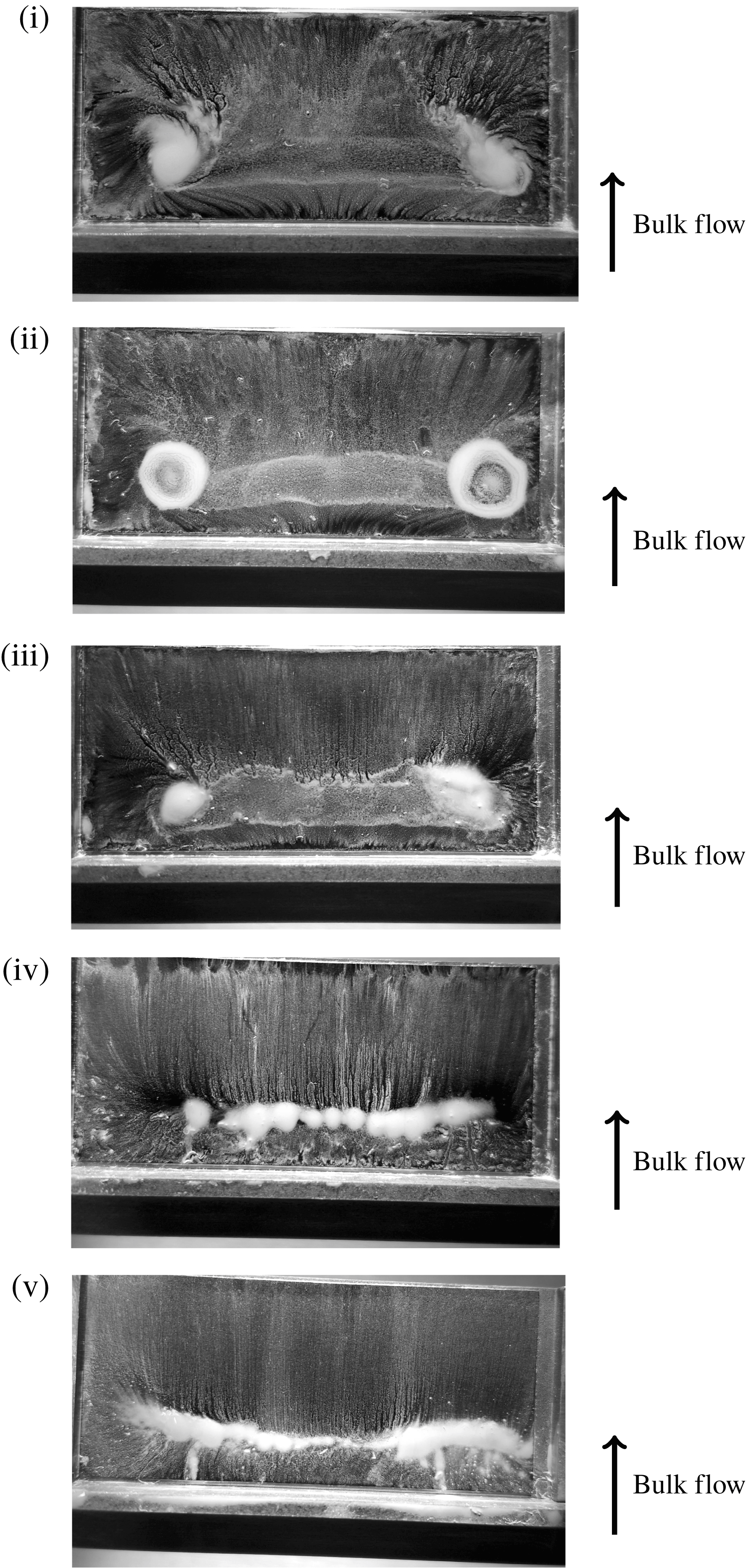
, respectively. Because an operating point is specified by flow rate, both the Reynolds and Mach numbers are simultaneously varied. For reasons that will become apparent in § 5 Mach number has been chosen as the abscissa. Five specific Mach numbers (marked i to v) are highlighted in each spectrogram. These correspond to the flow-visualisation results presented in figures 14 and 15.
When
 $l/d=2$
(a,c) the mode-I peak disappears when
 $M_{b}>0.26$
and only mode-II remains. This is the phenomenon that Ford et al. (Reference Ford, Winroth and Alfredsson2018) refer to as lock-on. Mode-I reappears again when
 $M_{b}>0.38$
. When
 $l/d=1.5$
(b,d) mode-I exists at all tested Mach numbers. Mode-II appears at similar flow conditions, but has an order of magnitude smaller amplitude than for
 $l/d=2$
(at least during lock-on).
(a,b) Spectrograms for geometries:
 $l/h=4.5$
,
 $l/d=2$
and
 $l/h=3.375$
,
 $l/d=1.5$
. (c,d) Associated modal amplitudes for (a) and (b), respectively. Operating conditions at which oil-film visualisations were obtained are indicated i–v.

Oil-film flow visualisation (CICERO). Geometry:
 $l/h=4.5$
,
 $l/d=2$
. (i)
 $M_{b}=0.15$
, (ii)
 $M_{b}=0.19$
, (iii)
 $M_{b}=0.23$
, (iv)
 $M_{b}=0.28$
, (v)
 $M_{b}=0.36$
.
Oil-film flow visualisation (CICERO). Geometry:
 $l/h=3.375$
,
 $l/d=1.5$
. (i)
 $M_{b}=0.15$
, (ii)
 $M_{b}=0.19$
, (iii)
 $M_{b}=0.22$
, (iv)
 $M_{b}=0.30$
, (v)
 $M_{b}=0.35$
.

Five flow-visualisation images (
 $l/d=2$
) are presented in order of increasing Mach number in figure 14. Initially, there is a clear indication of the TAV. Increasing the Mach number, as in figure 14(iii), causes the vortex-root diameter to shrink and the vortex centres move towards the meridian plane. At this Mach number, the mode-I shedding process is beginning to deviate from its characteristic Strouhal number, owing to the onset of mode-II.
Figure 14(iv) is taken from a flow condition in which mode-I has ceased to exist at an independent frequency. The flow pattern differs vastly from (i–iii). The TAV-roots are not visible, instead a stagnation line can be seen parallel to the step. A similar flow pattern is shown in figure 14(v). The stagnation line extends across the whole width of the tail.
A summary of key parameters derived from the images in figure 14 is provided by table 2.
Summary of key parameters taken from surface visualisation (
 $l/h=4.5$
,
 $l/d=2$
).
 $\unicode[STIX]{x1D705}$
is the vortex scale,
 $x_{\unicode[STIX]{x1D705}}$
is the streamwise position from the shedder step,
 $\unicode[STIX]{x0394}z_{\unicode[STIX]{x1D705}}$
is the spanwise separation of the vortex roots.
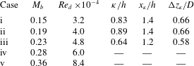
Figure 15 shows an equivalent set of images for the
 $l/d=1.5$
geometry. Generally, the clarity of the TAV is less distinct than when
 $l/d=2.0$
, probably because the geometry lies closer to the limit of the TAV region (refer back to figure 12) and the TAV may be intermittent.
The TAV is clearly observed in (i). Increasing the Mach number (ii) causes the TAV to become less clear. However, the presence of a band-like region of flow-visualisation paint between the anticipated locations of the vortex centres indicates that the TAV is at least periodically present. It is marginally shorter in spanwise extent than in (i).
Increasing the flow rate further (iii) causes an increase in the amplitude of mode-II and, although mode-I remains, a significant decrease in the mode-I Strouhal number occurs. The TAV structure becomes disrupted and indistinct, although some characteristics clearly remain. At (iv) mode-II begins to diminish in amplitude and mode-I begins to return to its former Strouhal number. Correspondingly, there is a distinct return towards a TAV-style flow pattern, particularly visible on the right-hand side of the image.
The final image (v) clearly shows the TAV vortex structure. At this Mach number, mode-II has diminished in magnitude and therefore the flow is likely to be moving into a ‘mode-I-dominated’ regime.
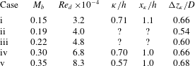
A summary of key parameters derived from the images in figure 15 is provided by table 3.
Summary of key parameters taken from surface visualisation (
 $l/h=3.375$
,
 $l/d=1.5$
).
 $\unicode[STIX]{x1D705}$
is the vortex scale,
 $x_{\unicode[STIX]{x1D705}}$
is the streamwise position from the shedder step,
 $\unicode[STIX]{x0394}z_{\unicode[STIX]{x1D705}}$
is the spanwise separation of the vortex roots. ? indicates uncertain measurement.
Both sets of flow-visualisation images suggest that the mode-I shedding behaviour of long-tailed geometries (
 $l/d>1$
) is characterised by the presence of a tail-attached vortex. When mode-I is disrupted by mode-II (mode interaction) the TAV structure breaks down. The greater the deviation from the characteristic Strouhal number, the greater the impact is on the TAV structure, categorically linking the TAV formation to mode-I.
It is interesting to note that although Ruderich & Fernholz (Reference Ruderich and Fernholz1986) report a near identical ‘TAV’ flow pattern for a T shaped shedder in low confinement (
 $d/D\leqslant 0.1$
), they do not report its sensitivity to flow conditions. The flow-visualisation data were obtained at
 $Re_{d}\approx 3\times 10^{4}$
and the authors state that results are uninfluenced by any further increase in Reynolds number (for values up to
 $Re_{d}\approx 4\times 10^{5}$
). Though the experiments of Ruderich & Fernholz (Reference Ruderich and Fernholz1986) cover a similar range of Reynolds numbers, the low confinement and low Mach number (
 $M_{b}<0.05$
) make it unlikely that mode interaction would have occurred. Thus the TAV pattern would not have been disrupted as it is in the present set of experimental results.
5 Mode-II
In this section it will be shown that mode-II has a different scaling behaviour as compared to mode-I. The onset of mode-II is dependent on Reynolds number and the Strouhal number primarily depends on the dimensionless pressure gradient. This is a function of the shedder geometry and the Mach number.
It is postulated that the presence of the vortex shedder induces a periodic separation at the pipe wall and this is responsible for the mode-II frequency. Ford et al. (Reference Ford, Winroth and Alfredsson2018) demonstrate numerous pieces of evidence for this; a reduction in near-wall Mach number downstream of the shedder when mode-II is present, for example.
It is thought that the separation results from the rapid acceleration and subsequent abrupt expansion of flow passing over the shedder body. Accordingly, it is a direct consequence of confinement. The initial rapid acceleration creates a thinning of the approaching boundary layer. In this case, the acceleration is so aggressive that relaminarisation of the approaching wall boundary layer is likely. A spatial acceleration parameter (
 $K$
) is presented by Schlichting (Reference Schlichting1960) as a means of determining when relaminarisation is possible, viz
 $$\begin{eqnarray}\displaystyle K(x)={\displaystyle \frac{\unicode[STIX]{x1D708}}{U^{2}}}{\displaystyle \frac{\unicode[STIX]{x2202}U}{\unicode[STIX]{x2202}x}}\geqslant 3.5\times 10^{-5}. & & \displaystyle\end{eqnarray}$$
The velocity gradient term may be estimated as sonic conditions are realised over the shedder when
 $M_{b}\approx 0.4$
, see Ford et al. (Reference Ford, Winroth and Alfredsson2018). Assuming the acceleration is linear across the geometry (likely an underestimate of the reality),
 $K$
is an order of magnitude larger than required by the relaminarisation criterion (5.1). At the lowest flow rate, the peak velocity is conservatively estimated from the geometric blockage of the shedder alone;
 $K$
is then approximately 2.5 times the critical value for relaminarisation.
This relaminarisation process may well explain the apparent insensitivity of modes I and II to the upstream pipe length, as indicated previously in § 2.1. The conditions over the shedder are essentially set by the shedder itself, desensitising it to the approaching velocity profile.
Separation at the pipe wall has also been observed in several other confined bluff-body studies. Venugopal, Agrawal & Prabhu (Reference Venugopal, Agrawal and Prabhu2018) present a numerical/experimental investigation of the shedding behind a confined trapezoidal shedder (
 $d/D=0.28$
), across a large range of Reynolds numbers (
 $60<Re_{d}<0.6\times 10^{5}$
). The study explicitly highlights interaction between the shed vortices and the pipe wall. The numerical study shows the potential for the wall boundary layer to be in a separated state in the proximity of the shedder maximum thickness, even at low Reynolds number (
 $Re_{d}\approx 140$
). Similarly, a wall separation is indicated by Yu et al. (Reference Yu, Leung, Lu, Cheng and Chan2011) for a relatively aerodynamic shedder at a blockage ratio of 0.5 and
 $Re_{d}\approx 6\times 10^{3}$
.
The form of the bluff body influences the onset Reynolds number for mode-II. More aerodynamic forms appear to delay the onset of the wall separation. As will be seen, this is borne out by the data of the present study, wherein mode-II first appears at higher Reynolds numbers for geometries with longer tails.
Assuming that mode-II is connected to the viscous-dominated wall flow, it is sensible that the onset occurs at similar Reynolds numbers in the two rigs. This is demonstrated by two example frequency spectrograms in figure 16. The spectrograms are plotted as a function of Reynolds number, with labelled iso-lines of Mach number overlaid. Mode-II is observed in the CICERO data when
 $Re_{d}>1.6\times 10^{4}$
(
 $M_{b}>0.08$
). In the NT rig, mode-II appears when
 $Re_{d}>2.4\times 10^{4}$
(
 $M_{b}>0.02$
).
Spectrograms for no-tail geometries: (a) CICERO rig, (b) NT rig.

Furthermore if the frequency of mode-II is related to an unsteady boundary-layer separation, then the ratio of mode-II frequencies should be close to the scale ratio of the CICERO and NT rigs. Figure 17 shows the frequency ratios between the CICERO and NT rigs for all observations of mode-II at Reynolds number matched condition. As can be observed the ratios closely approximate the physical scale ratio of the rigs.
Mode-II frequency ratio between CICERO and NT rigs at Reynolds matched conditions.

The parameters determining the frequency of mode-II are likely to be similar to those connected to ordinary boundary-layer growth, i.e. the level of confinement, the fluid viscous properties and the pressure gradient (which is set up by the shedder body). Taking a dimensional analysis approach, one may write
 $$\begin{eqnarray}\displaystyle f_{II}=f\left(U_{b},d,D,\unicode[STIX]{x1D70C}_{b},\unicode[STIX]{x1D707}_{b},\left.\frac{\unicode[STIX]{x2202}p}{\unicode[STIX]{x2202}x}\right|_{max}\right). & & \displaystyle\end{eqnarray}$$
Taking the velocity (
 $U_{b}$
), density (
 $\unicode[STIX]{x1D70C}_{b}$
) and shedder diameter (
 $d$
) to be characteristic scales of time, mass and length, respectively, three dimensionless groups are found
 $$\begin{eqnarray}\displaystyle \frac{f_{II}d}{U_{b}}=St_{II}=f\left(Re_{d},\frac{d}{D},\unicode[STIX]{x1D6FD}\right), & & \displaystyle\end{eqnarray}$$
where
 $\unicode[STIX]{x1D6FD}$
is the dimensionless axial pressure gradient,
 $$\begin{eqnarray}\displaystyle \unicode[STIX]{x1D6FD}=\frac{d}{\unicode[STIX]{x1D70C}_{b}U_{b}^{2}}\left.\frac{\unicode[STIX]{x2202}p}{\unicode[STIX]{x2202}x}\right|_{max}. & & \displaystyle\end{eqnarray}$$
The velocity in (5.4) may be substituted for the Mach number to yield
 $$\begin{eqnarray}\displaystyle \unicode[STIX]{x1D6FD}=\frac{1}{M_{b}^{2}\unicode[STIX]{x1D6FE}}\left.\frac{d}{p_{b}}\frac{\unicode[STIX]{x2202}p}{\unicode[STIX]{x2202}x}\right|_{max}. & & \displaystyle\end{eqnarray}$$
The axial pressure gradient is principally a function of the geometry and here the geometry is non-dimensionally identical between the two rigs. The operating pressure is also similar (
 $p_{b}/p_{amb}\lesssim 1.3$
for all CICERO experiments). The working fluid is the same and hence
 $\unicode[STIX]{x1D6FD}$
reduces to a function of
 $M_{b}$
, viz
 $$\begin{eqnarray}\displaystyle \unicode[STIX]{x1D6FD}\propto M_{b}^{-2}. & & \displaystyle\end{eqnarray}$$
Hence, in this case, the dimensionless groups governing the behaviour of mode-II are blockage ratio, Reynolds number and Mach number. Note that the blockage ratio is held constant in the present set of experiments and is hence an inactive parameter. The final expression for the Strouhal number becomes
 $$\begin{eqnarray}\displaystyle St_{II}=f\left(Re_{d},M_{b};\frac{d}{D}\right). & & \displaystyle\end{eqnarray}$$
Figure 18 plots the mode-II Strouhal number a function of Reynolds number (a) and Mach number (b). Mode-II emerges at similar Reynolds numbers in the two rigs, although there is a remaining dependence on the specific geometry; longer-tailed geometries delay the onset.
Mode-II Strouhal number. All geometries have
 $h/d=0.44$
(
 $h/d=0$
for
 $l/d=0$
).

Examination of figure 18(b) reveals that the Strouhal number is inversely proportional to the Mach number, viz
 $$\begin{eqnarray}\displaystyle St_{II}=\frac{k}{M_{b}}, & & \displaystyle\end{eqnarray}$$
where the constant of proportionality,
 $k$
, is a weak function of
 $l/d$
, as shown in figure 19.
Variation of the proportionality constant
 $k$
(5.8) as a function of tail length.

The mode-II Strouhal number begins to collapse to a single value for
 $M_{b}\approx 0.4$
. It is around this Mach number that the flow over the shedder body starts to become sonic. It may be the case that the presence of a shock wave over the body fixes the position and hence scale/frequency of the wall separation, leading to minimal variation as the Mach number increases further.
To further explore the effect of Mach number on mode-II Strouhal number, an additional experiment was conducted in the CICERO rig with the air heated to approximately
 $80^{\circ }\text{C}$
. This enabled the Mach number to be varied without any geometric alterations to the rig, isolating any potential influence of the NT/CICERO set-ups. Unfortunately this approach allowed only modest changes in Mach number across a limited Reynolds number range (due to the limit of heater output power). It was not possible to use the microphones to detect vortex shedding at
 $80^{\circ }\text{C}$
and therefore a Pitot pressure probe, positioned in the downstream boundary layer, was used instead. The Pitot probe measurement was verified by repeating the cold-flow case with both measurement techniques.
Figure 20 shows the mode-II Strouhal number as a function of Reynolds number (a) and Mach number (b). Again, the same trend is observed as in the NT/CICERO comparison: the length scale is principally sensitive to the Mach number. These results strongly suggest that the change in mode-II frequency observed in the NT rig is not a result of the specific set-up, or rig scale per se, but is a result of the difference in operating Mach number.
Mode-II Strouhal number,
 $l/d=2$
,
 $l/h=7.2$
under hot- and cold-flow conditions.
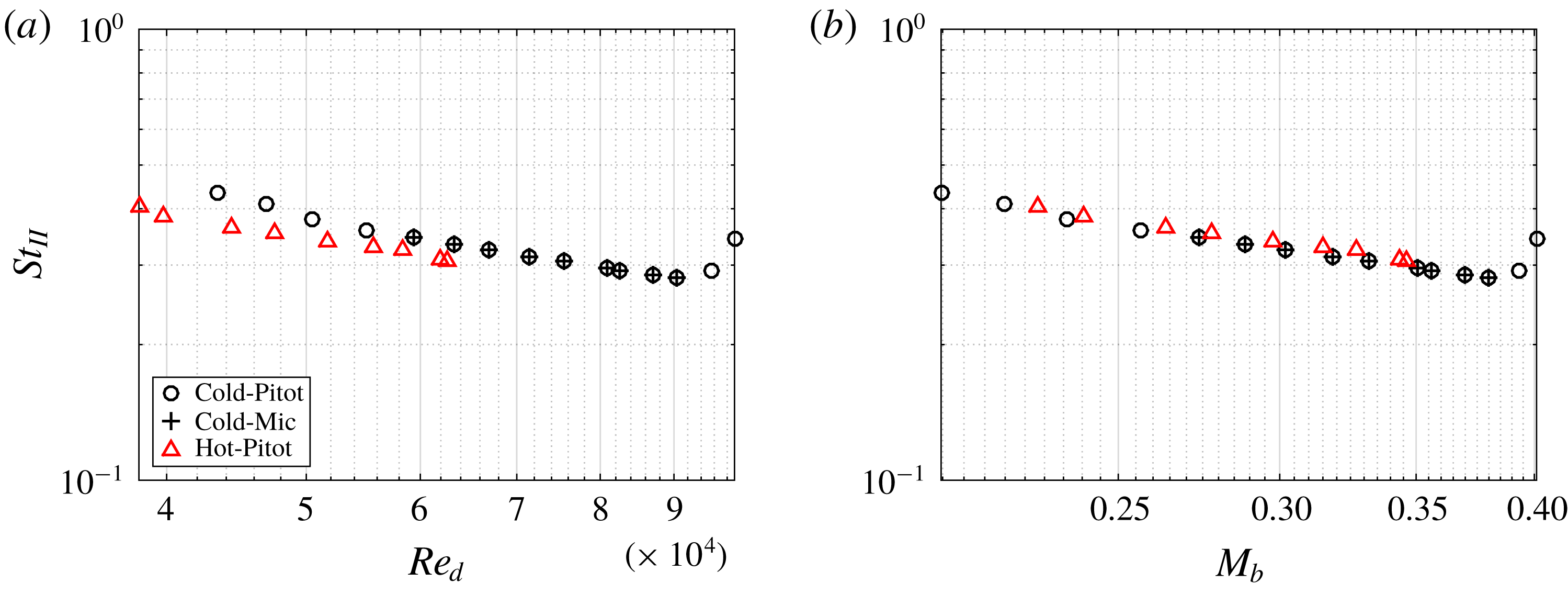
This result is important, because it suggests that matching Reynolds number alone is insufficient to guarantee dynamic similarity of confined bluff-body flows. For sufficiently high Reynolds number, the dimensionless mode-I frequency is essentially constant. Thus, the ratio of modal frequencies is also inversely proportional to the Mach number, viz
 $$\begin{eqnarray}\displaystyle \frac{f_{II}}{f_{I}}\propto M_{b}^{-1}. & & \displaystyle\end{eqnarray}$$
Therefore, scaling a rig up in physical dimension, and matching Reynolds number will result in an increase in the scale separation of modes-I and II. This does not prohibit the ratio of frequencies from becoming an integer. However, mode interaction is prevented on the second criterion of Ford et al. (Reference Ford, Winroth and Alfredsson2018) by limiting the ratio of length scales and ensuring the flow field is always mode-I dominated. Of course the corollary is also true, if one scales a rig down in size.
Mode interaction is clearly an important factor in confined bluff-body flows, which may lead to the complete disruption of the principal shedding mode. Using the hypothesis for the interaction mechanism laid out by Ford et al. (Reference Ford, Winroth and Alfredsson2018) and the observations of the scaling behaviour of mode-II presented in this section allows a more complete picture of how to avoid (or indeed encourage) mode interaction.
It may be assumed that as the confinement ratio drops, mode-II will ultimately cease. The blockage ratio has not been explored as part of this study, but it is clearly an essential parameter. Further work is needed to establish the limits of the confined flow case. Certainly the existence of mode-II and the potential for mode interaction must form part of the definition of confinement for bluff-body flows.
6 Summary and conclusions
A series of experiments have been conducted to illuminate the wake-shedding behaviour specific to confined bluff bodies. Two Reynolds number matched facilities were used, at two geometric scales with a ratio of almost 1 : 5. The bluff body had a constant forebody geometry onto which splitter plates of different lengths and thicknesses were mounted.
The primary-shedding mode (mode-I) has a Strouhal number which is similar between the two rigs. It was shown that the Mach number strongly influences the variation in mode-I Strouhal number, especially in the case of short-tailed geometries.
Flow visualisation, both on the surface of the shedder tail and via smoke injection, was used to identify the topology of the wake. When the tail is sufficiently long, the primary vortex anchors to the tail, forming a single hoop-like structure (the so-called TAV). This pattern seems to be similar to those observed by Ruderich & Fernholz (Reference Ruderich and Fernholz1986) in a study conducted in much larger aspect ratio wind tunnel.
The appearance of the TAV depends on the non-dimensional length of the tail. It is postulated that the tail length should be at least three times the primary-vortex scale for the TAV topology to exist. This criterion means that short tails are unable to host the TAV, providing a topological reason for the observed difference in behaviour between long and short geometries.
Above a certain Reynolds number, which depends on the shedder geometry, a second mode (mode-II) appears. This mode was first reported by Ford et al. (Reference Ford, Winroth and Alfredsson2018). The dimensionless frequency (and hence length scale) of mode-II was shown to scale with Mach number. The tail length influenced the rate of growth of the mode-II Strouhal number.
In the smaller-scale CICERO rig, modes I and II can interact under certain conditions. This causes mode-I to lock-on to the mode-II frequency. It was demonstrated, via flow visualisation, that the TAV topology is disrupted during lock-on.
The existence of mode-II is, perhaps, the defining feature of a confined bluff-body flow. However, before the work of Ford et al. (Reference Ford, Winroth and Alfredsson2018) it has remained unreported. This is likely because the relatively few studies of confined bluff-body flows are conducted either at large scale or in water, wherein the Mach number is very low. Consequentially, the mode-II frequency is relativity small in amplitude and substantially separated in frequency from mode-I and thus likely to escape attention. However, it has been shown that mode-II can have substantial consequence for the entire flow topology of the confined bluff-body flow. By identifying the scaling behaviour of mode-II, this paper has identified the reason mode-II has remained so elusive. Further work is now required to establish the limits of the definition of confinement (with respect to bluff-body flows) by considering the presence or absence of a mode-II frequency.
Acknowledgements
C.F. gratefully acknowledges the financial support of the Lars-Erik Thunholm Foundation. The support of the Competence Centre for Gas Exchange (CCGEx) is also gratefully acknowledged. The authors acknowledge the technical support of the workshop staff of the KTH Fluid Physics laboratory, and of Felima in designing and producing three-dimensionally printed shedders specifically for smoke-injection experiments. Lastly the authors particularly thank Professor H. Alfredsson for his many and continued efforts in improving this article.
Supplementary movies
Supplementary movies are available at https://doi.org/10.1017/jfm.2019.583.


 Open access

