1 Introduction
Partisan gerrymandering, the manipulation of legislative districts for political gain, distorts democratic representation and undermines confidence in government. The United States will next redistrict after the 24th Census in 2020–2022, and gerrymandering stands as a fulcrum in the balance of power between the parties. Most of the recent literature has framed this issue through the courts, with authors jockeying to assist the justices with a “manageable standard” for identifying gerrymanders (Grofman and King Reference Grofman and King2007; Stephanopoulos and McGhee Reference Stephanopoulos and McGhee2015). But after three decades seeking such a standard, the Supreme Court in Rucho v. Common Cause gave up the chase, ruling that partisan gerrymandering is a nonjusticiable, political question. Chief Justice Roberts concluded his opinion by noting that the legislative “avenue for reform established by the Framers, and used by Congress in the past, remains open” (588 U.S., 2019, 33). This paper focuses on that federal, legislative approach.
The Constitution gives Congress power over the “Times, Places and Manners of holding [its] Elections.” Historically, Congress used that power to regulate the form of constituencies in the House. The Apportionment Act of 1842 required that representatives be elected from contiguous, single-member districts (Cong. Globe 1842); subsequent Acts stipulated that districts be equipopulous (17 Stat. 28 1872) and compact (31 Stat. 733 1901). Those requirements were reiterated in 1911 (37 Stat. 13) but lost in 1929 (Cong. Rec. 1929). Though both houses revived them in 1967, the bill failed in conference (Cong. Quarterly 1968). In the past half-century, Congress has neglected its responsibility for fair districts, but the issue was reintroduced with the first House bill of the 116th Congress. (For a legal history, see Supplementary Appendices G and H.)
This paper evaluates the potential impact of reviving statutory regulation of the form of congressional districts. It provides credible tools for comparing districting objectives. I begin from the requirements as last enacted by Congress: equipopulation, contiguity, and compactness. Doing so, I immediately confront an old conceptual hurdle: what does it mean for a district to be “compact”? Equipopulation and contiguity have undisputed mathematical definitions, but there are dozens of formal alternatives for compactness. These definitions quantify the closeness of people within a district, the length of its perimeters, or the similarity of its shape to a circle (see Section 2 or Ehrenburg (Reference Ehrenburg1892), Forrest (Reference Forrest1964), Schwartzberg (Reference Schwartzberg1966), Grofman (Reference Grofman1985), Young (Reference Young1988), Hofeller and Grofman (Reference Hofeller, Grofman and Grofman1990), Niemi et al. (Reference Niemi, Grofman, Carlucci and Hofeller1990), Polsby and Popper (Reference Polsby and Popper1991), Reock (Reference Reock1961), Angel, Parent, and Civco (Reference Angel, Parent and Civco2010), Chambers and Miller (Reference Chambers and Miller2010), Fryer and Holden (Reference Fryer and Holden2011)). Which definition ought to be applied? Does it matter? Does a choice among algorithms or objectives amount to a political choice between parties?
I adopt a simplified—but constitutionally and historically justified—framing, in which Congress assumes wholesale control of the process. I focus on explicit procedures for strict maximization of objectives. This is how the courts have enforced equipopulation: exactly, not approximately. This simplifies the districting process; it treats the forms of congressional districts in the same mechanical terms as the apportionment of seats to states. I implement these procedures and objectives in flexible automated districting software, that is a core contribution of this paper. This software makes it possible to generate statewide plans for different districting objectives.
Automated districting is in a class of problems not exactly solvable with computers. The number of potential solutions is combinatoric in the number of inputs, so an exhaustive search for the unique, best solution is not possible. Computer scientists call this type of problem “NP-hard.” To make progress, heuristic, iterative strategies may be employed. Searches from random initializations (seeds) terminate at local, not global, extrema. Repeated initializations and searches allow for the assembly of a collection of high-quality maps for each version of compactness. This makes it possible to quantitatively evaluate the impact on representation of different explicit objectives and algorithms. The software created for this project is distinguished from earlier work by the diversity of objective functions implemented and by its ability to generate a larger number of plans for larger states than past projects. It builds on a long history of “automated districting,” stretching from Weaver and Hess (Reference Weaver and Hess1963) at the dawn of computation, to modern projects like Altman and McDonald (Reference Altman and McDonald2011) who wrote software but did not exercise it, and Fryer and Holden (Reference Fryer and Holden2011) who generated individual maps using “power diagrams.” More recently, Chen and Rodden (Reference Chen and Rodden2013, Reference Chen and Rodden2015) and Cho and Liu (Reference Cho and Liu2016) deployed automated districting procedures to generate “populations” of districts and measure if enacted plans were outliers with respect to these distributions. That work has shown that enacted plans are indeed outliers with respect to specific automatically generated distributions. But are all distributions of maps consistent?
For each map generated by the software, I evaluate districts’ practical characteristics by aggregating voting returns and constituent populations. This completes the translation of definitions of compactness into collections of maps and thence into distributions of practical outcomes. I construct these distributions in 10 states, based on available data. I demonstrate that the choice among compactness objectives and algorithms is not in itself a loaded, implicitly political issue. Even though the shapes of generated districts change between the definitions, the various methods treat the two parties consistently in terms of seat shares, vote shares, and the number of competitive races. I show how this consistency arises and how the “compact” maps compare to the status quo. The work thus departs from past reviews (like Niemi et al. Reference Niemi, Grofman, Carlucci and Hofeller1990) by suggesting that—in this context—compactness is well defined in practice. New legislation can and should make a compactness requirement procedurally rigorous. This legal clarity need not divide the parties.
Since I am investigating a federal, legislative reform that would supersede the existing law, the Voting Rights Act (VRA) does not apply. Still, minority representation matters and it would be affected by reform. Per the intent of Section 2 of the VRA, I evaluate the impact of a compactness requirement on minority representation. I use a single, representative definition of compactness to district the entire United States and find the net change in minority representation to be small. I briefly discuss alternative ways of framing this issue.
The methods presented are applicable and the conclusions on compactness pertinent, beyond the frame of a federal, legislative requirement. A majority of state constitutions require compact legislative districts, and such requirements have been the basis for successful litigation at the state level, as in League of Women Voters v. the Commonwealth of Pennsylvania. A number of states are also considering constitutional amendments to create independent commissions for redistricting. The methods of this paper facilitate data-driven debate over the meaning and implications of compactness, as both legal standards and as objectives for commissioners. At the federal level, establishing a claim of vote dilution in violation of Section 2 of the VRA requires litigants to demonstrate that a minority is “geographically compact” (the first of the Gingles preconditions). The methods here offer a determination of that compactness that is more realistic and sophisticated than existing approaches. More broadly, the courts have consistently enumerated compactness as a “traditional districting principle” but have struggled to enforce it since its formal meaning has been ill-specified.
It is also hoped that this software will help foster a more formal and quantitative debate over aspatial objectives—both in isolation and in tandem with the spatial ones presented here. Despite its wide use, some critics have argued that compactness is a poor (or incomplete) criterion (Grofman Reference Grofman1985). The automated software developed can be extended with formal objectives for other “traditional districting principles.” For example, the aim of respecting existing political subdivisions can be integrated as an objective in the software or used post hoc to evaluate districts (Appendix E). Maps with better prospects for minority candidates can be selected from an existing distribution (Appendix F).
Congress has enormous latitude over the forms of congressional districts. It was granted this power intentionally and explicitly by the founders, with the responsibility of ensuring uniform and unbiased regulation of representation (Kurland and Lerner Reference Kurland and Lerner2000). It has of late evaded this responsibility. This paper aims to revive interest in this power and responsibility by evaluating the impact of Congress picking up where it left off in 1967 and requiring compact districts. Districting via compactness would shift the partisan composition of the delegations of gerrymandered states like Maryland and North Carolina; these shifts are consistent across every formal definition of compactness considered in this project. On its own, compact districts would also carry a slight reduction in minority representatives.
Seen broadly, this paper offers a flexible tool and quantitative framework for evaluating trade-offs between formal districting objectives in legislative and academic debate.
2 Compactness
Compactness is a succinct proxy for proximity-based communities. It reflects the American norm of geographic representation for the House that, though not mandated by the Constitution, was clearly expected by the founders and is today required by statute. This section presents a number of common expressions for measuring compactness, which will be used as objective functions in the optimization procedure presented in Section 3.1. It describes some of their limitations, in that context. It also presents several stand-alone procedures or algorithms for generating compact districts.
2.1 Defining Compactness
In an early review of compactness, Niemi et al. (Reference Niemi, Grofman, Carlucci and Hofeller1990) remarked that it is “multidimensional.” As illustrated in Figure 1, the single word corresponds to many different notions. While a circle is broadly understood to be compact, shapes may be noncompact by being disperse (or distended), highly indented, or dissected. A single shape may be judged more or less compact based on the proximity of the elements it contains.
Various distinct “concepts” are associated with compactness. The circle is typically agreed to be the most compact shape, to which may be contrasted disperse, indented, or dissected ones. But one may also look “within” a shape. In the middle frame, the dots are less disperse if one shifts the cells from the thick black bounds to the dotted ones.

Each separate notion corresponds to a separate mathematical expression. Not all notions of compactness are created equal. In this work, I reject mathematical definitions that are not invariant under rotations or scaling. The compactness of a district does not change when measured in miles instead of kilometers or when surveyed with a compass instead of a sextant. This precludes concepts like the total perimeter of a district or the ratio of its North–South and East–West extents. I further require that each measure of compactness be normalized to 1 and that a larger number is always more compact. This requirement makes compactness comparable across states and districts with very different population density and makes it easier to combine it with other constraints, namely equipopulation.
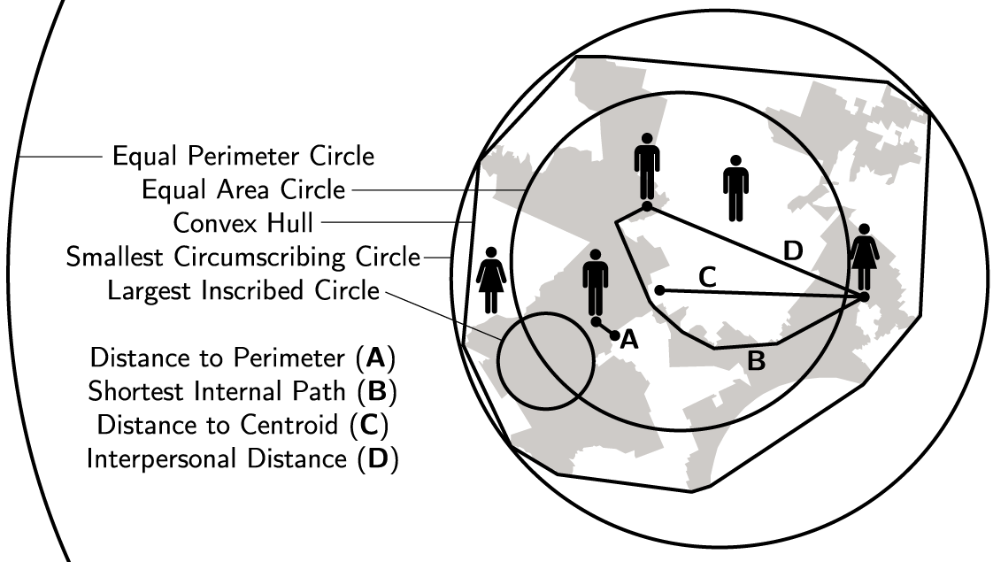
Most measures of compactness are composed of ratios of lengths, areas, or populations of the district, with respect to a reference shape derived from the district. Figure 2 illustrates the common reference shapes. Four circles are defined: the largest inscribed circle (LIC), the smallest circumscribing circle (SCC), and the circles of equal area and equal perimeter. I define the radius of the equal area circle  $R\equiv \sqrt{A/\unicode[STIX]{x1D70B}}$ and call the circle of radius
 $R$ centered at the district’s centroid
 $C_{R}$. The convex hull (CH) is defined as the smallest convex polygon that encloses a district; it is the shape a rubber band would make if wrapped around it.
Building blocks of compactness measures, on Pennsylvania’s 7th congressional district. From these derived shapes and lengths, a great number of measures may be defined.

For each shape, I denote its surface (or shape) by  $S$ and its area by
 $A$, the perimeter by
 $P$ and the length of that perimeter by
 $\ell$. The population contained within the shape is
 $p$. One may additionally define radii to the centers of population
 $\unicode[STIX]{x1D70C}_{p}$ or area
 $\unicode[STIX]{x1D70C}_{A}$ and distances to the perimeter
 $d_{P}$ or between two points
 $d_{ij}$. The shortest internal path
 $\unicode[STIX]{x1D6FF}_{ij}$ is the distance between two points, constrained to lie within the shape (see Figure 2). In what follows, I denote intersections by
 $\cap$ and averages by
 $\langle x\rangle$. I use subscripts to denote variants of these quantities, for the derived shapes.
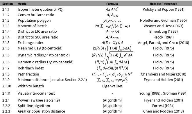
With these definitions in hand, it is straightforward to define “classical” compactness measures from various ratios. The measures are tabulated in Table 1 and described below.
Metrics of compactness, with formulas. See Section 2.1 for notation.

2.1.1 Isoperimeter Quotient
Perhaps the most famous measure of compactness is the isoperimeter quotient (IPQ); it is defined as the ratio of a shape’s area to that of a circle of equal perimeter. A circle of circumference  $\ell$ has area
 $\unicode[STIX]{x1D70B}(\ell /2\unicode[STIX]{x1D70B})^{2}=\ell ^{2}/4\unicode[STIX]{x1D70B}$, so the IPQ simplifies to
 $4\unicode[STIX]{x1D70B}A/\ell ^{2}$. In the districting literature, it is often attributed to Polsby and Popper (Reference Polsby and Popper1991), while
 $\text{IPQ}^{-1/2}$ is associated with Schwartzberg (Reference Schwartzberg1966). The IPQ is mainly sensitive to the perimeter; it responds little to broad deformations of the shape. It and other perimeter measures exhibit subtle definitional issues because geographic boundaries like coastlines often have “fractal” properties in the sense that their lengths depend on the scale at which they are measured. Nevertheless, the method is computationally simple, readily understood, widely used, and fairly performant. I drop a number of monotonic transformations of the IPQ (like the Schwartzberg measure).
2.1.2 Convex Hull Ratios
The convex hull may be used to define numerous metrics by dividing the areas or populations in the district with those in the hull. To recognize the existing geometry of the state (whose borders may not be compact), the population or area of the hull may be limited to citizens or land within the same state. I implement the area ratio  $A/A_{CH}$ and “population polygon” method
 $p/p_{CH,\,\text{state}}$. These typically privilege convex shapes and result in maps with clean, convex districts that may however be fairly disperse or “long.”
2.1.3 Moments of Inertia
The moment of inertia  $I$ is a dispersion measure defined by the weighted distances squared of the elements of a district to a fixed point. Weaver and Hess implemented its application to the districting problem as early as Reference Weaver and Hess1963. In this case, the weights
 $w_{i}$ of the cells are their populations or areas, and the fixed point considered is the center of mass (either area or population). For discrete elements
 $i$ on the surface
 $S$, this is
 $I=\sum _{i\in S}w_{i}\unicode[STIX]{x1D70C}_{i}^{2}$.
A uniform circular disk of equal area is typically used as the reference shape. The moment of inertia of such a disk with respect to its center is  $A\sum _{i}w_{i}/2\unicode[STIX]{x1D70B}$. For areal weights, this simplifies to
 $A^{2}/2\unicode[STIX]{x1D70B}$ and for a disk of population
 $N$, it is
 $NA/2\unicode[STIX]{x1D70B}$. Since large moments of inertia denote less compactness, the normalization is in the numerator:
 $2\unicode[STIX]{x1D70B}(\sum _{i}w_{i}\unicode[STIX]{x1D70C}_{i}^{2})/(A\sum _{i}w_{i})$.
2.1.4 Inscribed and Circumscribing Circles
In 1892, Ehrenburg proposed considering the ratio of a shape’s area to that of its LIC or SCC:  $A_{LIC}/A$ and
 $A/A_{SCC}$. Reock proposed the latter measure again in Reference Reock1961, and it sometimes bears his name in the districting literature. In practice, I have found that they require heavy-handed optimization with ad hoc “fixes” (see Appendix C.4.1). The problem is that any change to the shape that does not touch the circle is equivalent so that there is no penalty for “tentacles” and no “smooth path” toward a global minimum.
2.1.5 Exchange Index
Angel, Parent, and Civco (Reference Angel, Parent and Civco2010) propose to calculate “exchange” as the ratio of the areas of the intersection of an equal area circle centered at the district’s centroid, with the district itself:  $A(S\cap C_{R})/A$. The larger the fractional intersection, the more compact the shape. Because it privileges modifications to districts’ boundaries that place more of the area close to the center, the definition has a smooth “path” toward an optimal configuration and works well in automated settings. It is in some sense a dispersion measure.
2.1.6 Mean, Dynamic, or Harmonic Radius
The mean radius is the average value of the radius  $\unicode[STIX]{x1D70C}$ to the district centroid. The dynamic and harmonic radii instead express
 $\unicode[STIX]{x1D70C}^{2}$ and
 $1/\unicode[STIX]{x1D70C}$, respectively (Frolov Reference Frolov1975). All three are areal dispersion measures. Integrating the radius
 $\unicode[STIX]{x1D70C}$ over a surface
 $S$ of area
 $A$, the mean radius is thus
 $(\int _{S}\unicode[STIX]{x1D70C}\,dS)/S$, the dynamical radius is
 $\sqrt{(\int _{S}\unicode[STIX]{x1D70C}^{2}\,dS)/A}$, and the harmonic radius is
 $A/\int _{S}dS/\unicode[STIX]{x1D70C}$. Each of these may be normalized by the corresponding value for a circle of equal area:
 $2R/3$,
 $R/\sqrt{2}$, or
 $R/2$, respectively. Since radii larger than a circle’s are less compact, the normalizations go in the numerator.
2.1.7 Distance to Perimeter
The average distance from a point in a shape to its perimeter  $d_{P}$ is compared to a circle, for which the value is
 $R/3$. More-compact districts have less of their area close to the perimeter.
2.1.8 Path Fraction
Chambers and Miller (Reference Chambers and Miller2010) propose a measure of “bizarreness,” which reduces to the probability that the shortest in-state path between two people in the district, is itself contained within the district. The intuition is that a representative should not have to leave her district when driving from one voter to another. For people  $i$ and
 $j$, this is
 $(\sum _{i}\sum _{j}\lfloor d_{ij}/\unicode[STIX]{x1D6FF}_{ij}\rfloor )/N^{2}$.
2.1.9 Interpersonal Distance/Power Diagrams
Fryer and Holden (Reference Fryer and Holden2011) use the total distance squared between people. If the people are aggregated into cells (here, census tracts)  $i$ with populations
 $w_{i}$ and separated from neighbors
 $j$ by distance
 $d_{ij}$, this is
 $\sum _{i}\sum _{j}w_{i}w_{j}d_{ij}^{2}$. Fryer and Holden demonstrate that partitions that optimize this measure are additively weighted power diagrams (like a Voronoi diagram). Taking compact to mean “proximate,” they prove that these partitions are “optimally compact.” In Section 2.2.1, I describe an explicit algorithm for power diagrams, but a normalized measure may also be defined by dividing the average interpersonal distance by the corresponding value for a circle of equal area,
 $128R/45\unicode[STIX]{x1D70B}$.Footnote 1
2.1.10 Axis Ratio
The simple width to length ratio  $W/L$ is not very sensitive as a compactness measure: depending on the precise definition, a spindly “X” may be as compact as a square. But it is, in fact, used (at least, by Iowa) and it is readily calculable. The width and length may themselves be defined in a number of ways; I calculate
 $W/L$ as the ratio of the eigenvalues of the two principal components of the population point cloud in the projected geometry.
2.1.11 Visual Test
The visual test (Young Reference Young1988)—sometimes jokingly called the interocular (it hits you between the eyes—Grofman Reference Grofman1991) or obscenity test (“I know it when I see it,” per Potter Stewart)—is, in fact, a serious legal and diagnostic tool. Justice O’Connor wrote in Shaw v. Reno that “reapportionment is one area in which appearances do matter” (509 U.S. 630, 1993). Recently, Chou et al. (Reference Chou, Kimbrough, Sullivan-Fedock, Woodard and Murphy2012, Reference Chou, Kimbrough, Murphy, Sullivan-Fedock and Woodard2014) and Kaufman, King, and Komisarchik (Reference Kaufman, King and Komisarchik2017) have elicited visual feedback on district plans from both experts and laypeople to understand what people perceive as unfair.
Moreover, the visual test is an indispensable diagnostic for debugging and evaluating if the code for other metrics are “working.” In that sense, it represents my own inescapable bias for this project: it is the threshold where maps looked sensible.
It is worth acknowledging that there do exist definitions of compactness that are not included above. There is a limit to what is computationally feasible for automation. For example, Angel, Parent, and Civco (Reference Angel, Parent and Civco2010) define a “traversal index” by dividing the average length of internal paths between points on a district’s perimeter by the corresponding value for a circle. Computationally, this is simply too demanding. Evaluating this method would entail reevaluating the shortest paths for every potential move, which is computationally unfeasible.
Part of the aim of this research is to motivate a broad strategy for comparing formal and districting objectives. This project could well be extended by implementing additional spatial or aspatial objectives. This is illustrated briefly in Appendix E, for communities of interest.
2.2 Procedures
In addition to metrics—scalars that can be used as objective functions in an arbitrary optimization—a number of algorithms or procedures have been defined for generating a compact districting for a state.
2.2.1 Power Diagrams
The first of these algorithms is the power-diagram method discussed above (2.1.9). My implementation is similar to Fryer and Holden’s and proceeds as follows:
(1) Regions
 $r$ are defined by a center $\boldsymbol{x}_{r}$ and power $\unicode[STIX]{x1D706}_{r}$. The initial centers are chosen randomly and the initial powers are set to 0.
(2) Cells
$c$ located at $\boldsymbol{x}_{c}$ are assigned to region $r$ by $\text{argmin}_{r}(|\boldsymbol{x}_{r}-\boldsymbol{x}_{c}|^{2}-\unicode[STIX]{x1D706}_{r}^{2})$.(3) The region centers
$\boldsymbol{x}_{r}$ move slowly toward the region centroids and the powers $\unicode[STIX]{x1D706}_{r}$ increase or decrease so as to equalize the regions’ populations.


Steps 2 and 3 repeat until a convergence threshold is reached.
2.2.2 Split-Line Algorithm
The split-line algorithm iteratively splits the state’s regions. Regions (districts)  $r$ of population
 $p_{r}$ containing
 $s_{r}>1$ seats are split in two pieces of population
 $p_{r}\lfloor s_{r}/2\rfloor /s_{r}$ and
 $p_{r}\lceil s_{r}/2\rceil /s_{r}$, along the shortest possible line. This proceeds until each region has a single seat. The algorithm was first conceived by Forrest (Reference Forrest1964), and a slightly different approach is laid out by Spann, Kane, and Gulotta (Reference Spann, Kane and Gulotta2007).
2.2.3 Areal or Population Radii
For comparison purposes, I have included a distance-based assignment approach, similar to Chen, Rodden, and Cottrell (Reference Chen and Rodden2013, Reference Chen and Rodden2015, Reference Chen and Cottrell2016). In short, I trade cells between districts to minimize the cell’s squared distance to the population or area centroid. My method differs from theirs in that I weight the squared distances by the radius squared of the equal area circle (in other words, the area divided by  $\unicode[STIX]{x1D70B}$). This makes the algorithm scale-invariant. I also allow the algorithm to run long beyond population convergence to obtain more-compact districts. This approach can be naturally subsumed in the “general objective function” approach used for the other compactness scores.
This section has presented various meanings of compactness and reviewed existing mathematical definitions of the term. I now turn to deploying these definitions to algorithmically generate compact districts.
3 Automated Districting: The C4 Software
After each federal census, the states are apportioned representation in the House of Representatives proportional with their populations. The states are then tasked with assigning these seats to equipopulous, single-member districts of contiguous area.
This section presents this problem mathematically and describes the software implemented to address it computationally. This project differs from earlier catalogs of definitions and past efforts at automation in the diversity of objectives implemented. I am, therefore, able to quantitatively assess the practical impact of alternative definitions of compactness. Appendix B reviews past work on this problem.
3.1 The Constraint Problem
Formally, electoral districting is a graph partitioning problem. The task is to partition a set (state) into  $N$ nonoverlapping, contiguous, equipopulous regions
 $r$ (congressional districts), while optimizing the compactness of those regions. I do this using discrete cells
 $c$ of population
 $p^{c}$ (census tracts). Each cell is a node in the graph of the state, and the nodes are connected by edges if they are contiguous (share perimeter). The graph of the state itself must be connected: for any two nodes on the graph, there must exist a path between them. (See Appendix C.2 for details on islands and enclaves.)
The regions are then connected subgraphs of the state and partition it: every cell in the state must belong to exactly one region. I denote the set of cells (nodes) in each region by  $X^{r}$. The regions’ populations are the sum of their cells’ populations,
 $p^{r}=\sum _{c\in X^{r}}p^{c}$. The target population across regions
 $p_{\text{target}}$ is equal to the population of the state, divided by
 $N$. The compactness of a region is a function of its cells,
 ${\mathcal{C}}(X^{r})$. I will refer to the region that contains
 $c$ by
 $r(c)$.
The contiguity requirement is algorithmically enforced: no change that results in a disconnected graph for any region is ever considered. To formalize this, it is useful to define the set of nodes  ${X^{r}}^{\prime }$ that are not in
 $X^{r}$ but are adjacent to a node in it and are not themselves cut nodes of their current region (their removal would not break its connectedness). Considering a cell
 $c$ in
 ${X^{r}}^{\prime }$ and
 $X^{s}$, I then define the union of
 $X^{r}$ with one additional node
 $c$ by
 $X_{+c}^{r}\equiv X^{r}\cup \{c\}$ and the set with one node removed by
 $X_{-c}^{s}\equiv X^{s}\setminus \{c\}$.
The contiguity requirement is thus built in to the procedure. The equipopulation constraint and compactness objective are explicitly optimized using a greedy search that proceeds cyclically over the  $N$ regions.
Naïvely, one might define a combined objective function, incorporating the compactness and population count of each region. In each iteration, a region  $r$ would annex the cell
 $c\in {X^{r}}^{\prime }$ whose reassignment from its current region resulted in the largest improvement in the combined objective function of the two regions. Along these lines, the population objective for each region might then take the form
 ${\mathcal{P}}(p_{r})=-(|p_{r}/p_{\text{target}}-1|/\unicode[STIX]{x1D6E5})^{\unicode[STIX]{x1D6FC}}$, with
 $\unicode[STIX]{x1D6E5}$ an allowable tolerance from
 $p_{\text{target}}$ and
 $\unicode[STIX]{x1D6FC}$ a tunable parameter that I set to 4. The gradient of the population constraint would thus plummet as
 $p^{r}/p_{\text{target}}$ approached within
 $\unicode[STIX]{x1D6E5}$ of 1 (since the parenthesis is less than 1, raised to the fourth), but it would dominate the spatial part when
 $|p_{r}/p_{\text{target}}-1|>\unicode[STIX]{x1D6E5}$. One would then consider changes in this objective from moving a cell
 $c$ from region
 $r$ to
 $s$:
 ${\mathcal{P}}(p^{r}-p^{c})+{\mathcal{P}}(p^{s}+p^{c})$. This approach fails because the cells do not have equal population. Restricted to discrete trades, far from equilibrium, cells with larger population will always move first. Roughly speaking, the step size is much longer among more-populous cells but may not lead in the direction of steepest descent.
A small modification of the above suffices but comes at the price of an explicit objective function. I define the population difference function by
 $$\begin{eqnarray}{\mathcal{P}}(p^{r},p^{s})\equiv \text{sign}(p^{r}-p^{s})(|p^{r}/p_{\text{target}}^{r}-p^{s}/p_{\text{target}}^{s}|/\unicode[STIX]{x1D6E5})^{\unicode[STIX]{x1D6FC}}.\end{eqnarray}$$
This expression depends only on regions and is independent of cells. The population constraint thus impacts the choice of region to trade with, while the choice of cell along that border is left to the compactness scores  ${\mathcal{C}}$. As above, this term dominates the compactness measure when two regions’ population difference exceeds
 $\unicode[STIX]{x1D6E5}p_{\text{target}}$ but is very small when equipopulation is satisfied.
Each iteration on a region  $r$ culminates by its annexing the cell that maximizes the combined population and compactness function:
 $$\begin{eqnarray}\operatorname{argmax}_{c\in {X^{r}}^{\prime }}[{\mathcal{P}}(p^{r},p^{r(c)})+{\mathcal{C}}(X_{+c}^{r})-{\mathcal{C}}(X^{r})+{\mathcal{C}}(X_{-c}^{r(c)})-{\mathcal{C}}(X^{r(c)})].\end{eqnarray}$$
The optimization procedure begins by seeding the  $N$ regions with
 $N$ random cells, and the regions initially grow by subsuming unassigned cells
 $u$. Since the unassigned area has target
 $p_{\text{target}}^{r(u)}=0$, the population score to transfer out of it is infinite. In practice, I replace this score with a large number so that the
 $\operatorname{argmax}$ is well defined, but the behavior is unaltered: the regions quickly converge to cover the state. The procedure thus partitions the state while respecting the contiguity of regions and optimizing for equipopulation and compactness.
I also implement a modification of this procedure. In addition to one-directional moves, it is efficient to be able to trade cells between regions. If this functionality is activated, one trade is allowed per cycle, for which  $c\in {X^{r}}^{\prime }$ and
 $c^{\prime }\in ({X^{r(c)}}^{\prime }\cap X^{r})$ yield the largest gain in compactness:
 $$\begin{eqnarray}\operatorname{argmax}_{c,c^{\prime }}[{\mathcal{C}}(X_{+c,-c^{\prime }}^{r})-{\mathcal{C}}(X^{r})+{\mathcal{C}}(X_{-c,+c^{\prime }}^{r(c)})-{\mathcal{C}}(X^{r(c)})].\end{eqnarray}$$
3.2 Computational Implementation
A core contribution of this project is the software used to generate optimized districting plans. The software is called C4, for “contiguity-constrained clustering in c++.” C4 is open-sourced and freely available on GitHub. Key features are presented in greater detail in Appendix C.
To begin, a user loads the cells for a state along with their adjacency matrix (shared perimeters). To be able to enforce contiguity, the statewide plan must initially be connected; islands’ connections to the mainland may be specified explicitly, but C4 also has a module to handle this automatically. C4 also subsumes regions that are connected to the main graph by a single cut vertex since it is definitionally impossible to reassign the cut vertex without breaking contiguity.
The search then begins with a random draw without replacement of one cell for each region. The hill-climbing procedure detailed above then begins. Critical to the algorithm’s performance is its enforcement of region contiguity using integer programming. This is done by requiring that any cell removed from a region leave its neighbors in a single, connected subgraph. The search terminates after a configurable number of cycles with no improvement.
The software includes several of the standard metaheuristic strategies. Tabu lists (Glover Reference Glover1989) are, in fact, used for some compactness objectives, with individual cells precluded from moving for a fixed number of iterations after reassignment. I further implement two nonstandard procedures. First is a “de-stranding” method that removes strands of cells that cannot be removed by the cell-by-cell search. Second is a method for restarting the search by splitting in two the region with the worst compactness score and merging two other regions. Still, users should note that the software makes no guarantees in regard to the global optimality of solutions; such is the nature of NP-hard problems.
4 Spatial, Demographic, and Electoral Data
This section describes the required geographic, demographic, and election data. Geographic and demographic data are drawn from the US Census Bureau. Electoral data are far less standardized. I rely on both past efforts to assemble precinct-level returns as well as some data directly from the states.Footnote 2
4.1 Spatial and Demographic Data
The fundamental cells for map generation are 2015 census tracts. The geometries used are the census’s cartographic boundary shapefiles, and tract populations are from the 2015 American Community Survey (US Cenus Bureau 2016, 2018). I have generated topologies from each state geometry using PostGIS 2.1. To reduce perimeter measures’ sensitivity to highly indented (fractal) perimeters as along waterways, I have simplified the edges of the topology. The simplification is nominally to the 10 km level; however, if this would result in a new intersection (node/face/edge), the simplification threshold is successively halved until no intersection would result. For optimization and analysis, I project each state into its local EPSG coordinate reference system—usually a transverse Mercator or Lambert conformal conic, but sometimes Albers equal area projection. The datum is NAD83(HARN) and the units are meters. In states with multiple local projections, I select the centermost one. The list is derived from spatialreference.org and is included with the replication materials (Saxon Reference Saxon2019).
For comparisons with historical congressional districts, I have used the 107th, 111th, and 114th Congresses, which were drawn after the last three censuses (US Cenus Bureau 2012a, 2013a, 2015).
4.2 Election Returns
I employ precinct-level returns for presidential elections mapped by Ansolabehere and Rodden (Reference Ansolabehere and Rodden2011a,Reference Ansolabehere and Roddenb) for Florida (2008) and Illinois (2008). For Maryland (2008), Pennsylvania (2000–2012), and Texas (2000–2008), I have merged election returns by Ansolabehere, Palmer, and Lee (Reference Ansolabehere, Palmer and Lee2015) with Voter Tabulation Districts from the Census (2010) and Texas (2016). For Pennsylvania in 2012, the precinct names were slightly inconsistent; manual corrections and (human-verified) “fuzzy” matches were necessary. I supplement these with data directly from the states for Illinois (2016), Louisiana (2012, 2016), Maryland (2016), Minnesota (2008–2016), North Carolina (2012, 2016), Tennessee (2016), Texas (2012–2018), and Wisconsin (2004–2016) (Texas Legislative Council 2008, 2014, 2016, 2017, 2018; Minnesota Geographic Information Services 2009, 2016, 2017; Louisiana House of Representatives 2012, 2016; Louisiana Secretary of State 2012, 2016; North Carolina State Board of Elections 2012, 2013, 2016a,b; Tennessee Comptroller of the Treasury 2012; Tennessee Secretary of State 2016; Wisconsin Legislative Technology Services Bureau 2017, 2018; Illinois State Board of Elections 2017). For Maryland in 2016, the polling places and not precincts were available; I therefore use the former. The Illinois precincts have changed significantly since the 2010 Census release, and I have updated the precincts for Cook, DuPage, and Lake Counties (DuPage County GIS 2016; Ferruzzi Reference Ferruzzi2016; Lake County, Illinois 2016; Levy Reference Levy2016). Together, these cover most of the changes and more than half of the state’s population. The rest of the state is matched by precinct and county name. In Louisiana, North Carolina, and Tennessee, where early, absentee, and provisional voting are recorded at the county level, I divide these votes among precincts in proportions equal to the polling-place share of the county vote for each party.
5 The Political Consistency of Compactness Definitions
This section contrasts the spatial and political characteristics of maps generated with the C4 software with those from enacted plans. For this work, the fundamental cell size is the census tract, and equipopulation is required at the 2% level (with a few exceptions, below). Readers may object that federal law allows districting at the census block level and that the Supreme Court has rejected any de minimis threshold of equipopulation. These choices have the obvious advantage of speeding up the computation, though most of the algorithms work fine at the block group level. But they should also be considered in the context of the legislative approach that motivates this paper. Census tracts are designed to encapsulate relatively homogeneous populations, and their use can be thought of as a minimal regard for “preservation of communities.” When Congress last considered legislation to require equipopulous districts in 1967, it was at the 10% level—a looser threshold in better balance with other districting objectives (Cong. Quarterly 1968). As to the Court’s enforcement of its “one-person, one-vote” doctrine, it would be faced with Congress’s explicit Article 1, Section 5 authority over the elections and qualifications of its members.
I have generated a thousand maps per measure for each state for which I have voting data, using distributed computing. The exceptions are the path fraction, where I have generated only 280 maps per state, and the split-line algorithm, which is deterministic and yields a unique solution per state. The optimization procedures do sometimes fail to converge within population tolerance; the following analyses are therefore restricted to those maps with population deviations less than 2%. The population convergence issue is more acute with the axis ratio method and for Texas, and in these cases, I allow a 5% deviation; for axis ratio maps of Texas, a 10% threshold is allowed. The split-line algorithm generates a 2.1% deviation in Illinois and that solution is retained.
One must be precise about the statistical nature of this collection of maps. The algorithms are initialized by selecting one cell (census tract) to seed each district, without replacement. This is a bona fide random draw. Each state’s seeds are generated 50 times; each seed is “restarted” 20 times, resulting in different solutions. The optimized districts are, of course, not random.
After some general observations about the visual consistency of methods, I analyze the consistency of the compactness measures in two ways. First, I study the political outcomes of the populations of “optimized” maps: the seat share and competitiveness. I then turn briefly to the potential impacts for minority representation.
5.1 Observations on Optimized Maps
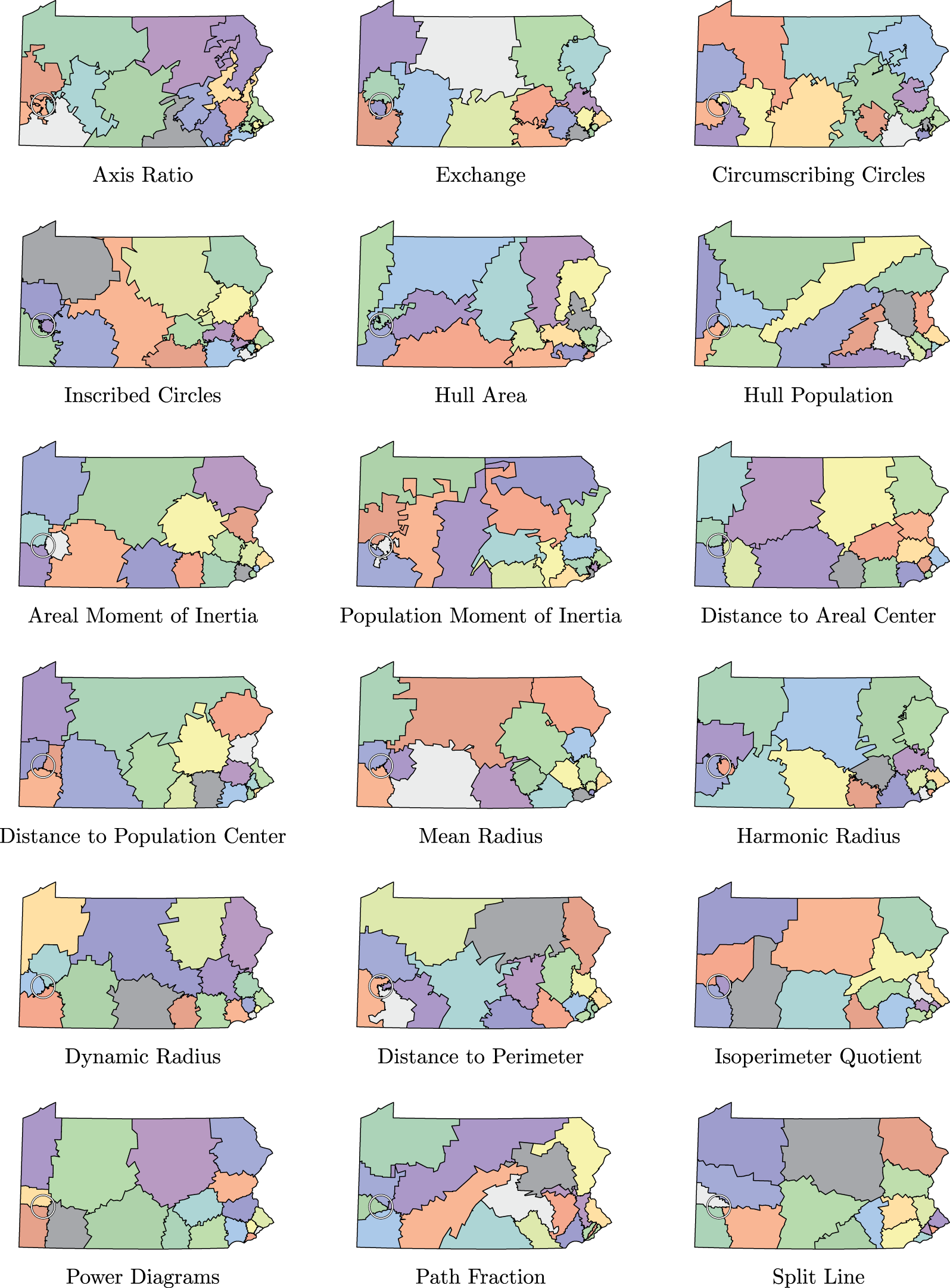
In Figure 3, I present a representative collection of maps drawn from a single seed. Additional plans can be explored interactively, online. Differences between methods emerge as expected. Axis ratio is simply ineffective. The IPQ contains “somewhat lumpy” shapes with smooth perimeters. The hull-based measures, along with the power-diagram and split-line algorithms, produce convex shapes with straight lines. It is interesting to consider the nontrivial relationships between the many methods. Power diagrams imply convex shapes that would result in good scores for hull population or hull area, but the converse is not necessarily true: convex shapes can be very distended (disperse) while power diagrams usually are not. A convex shape will contain all of the paths between people in the district and will therefore have a “path fraction” of 1 (Section 2.1.8), and a shape with a perfect “path fraction” likewise implies a high CH population ratio (Section 2.1.2), but the paths through phase space toward these optima are not generally the same.
Representative districting plans of Pennsylvania for various metrics. The treatment of Pittsburgh, halfway down in the western part of the state, evidences how optimizing according to different definitions of compactness results in different treatment of cities.

Across measures, the varying treatment of Pittsburgh is particularly notable: some algorithms divide it in many pieces (distance to the areal center or split line), while others cut a circle around the city (exchange, harmonic radius, or inscribed circles). It is this variation in the treatment of urban (in America, Democratic) voters that raises the possibility of bias from compactness. Is choosing an objective equivalent to choosing a winner?
5.2 The Political Consistency of Optimized Maps
The seat share and competitiveness of simulated districts are derived by reaggregating precinct-level voting data from presidential elections, described in Section 4. Presidential elections are used to avoid uncontested races and reduce incumbency effects. The procedure depends on consistency between presidential and congressional races. It is also an approximation in the sense that local candidates could better tack to individual constituencies, and even change their strategies as a function of the district lines. To mitigate this concern, multiple elections are presented when available to give a sense of geographically realistic distributions with different statewide vote shares.
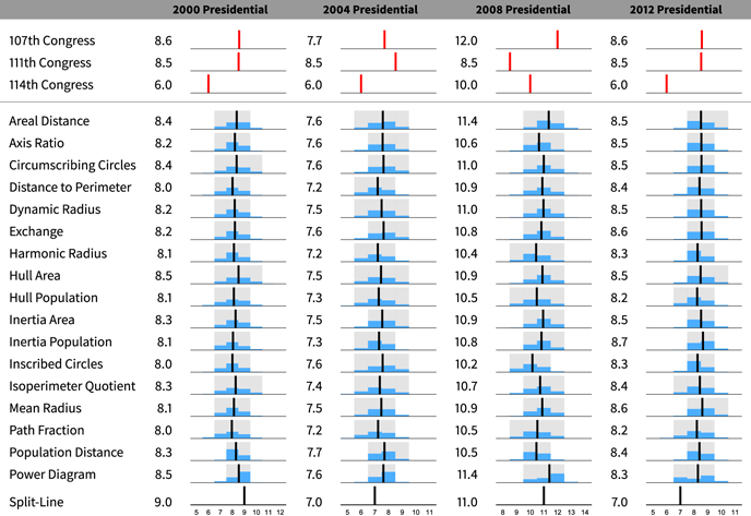
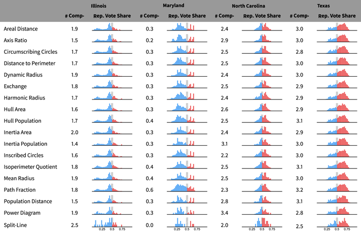
Each individual map results in a certain number of projected wins for Republicans and a complementary number for Democrats; each measure’s population of maps thus corresponds to a distribution of seats for each election. The same procedure is followed for the actual enacted maps from the last three districting cycles. In this way, the internal consistency of the simulated maps may be evaluated and as a group contrasted with the enacted maps. Results are shown for four elections in Pennsylvania in Table 2. The other nine states—Florida, Illinois, Louisiana, Maryland, Minnesota, North Carolina, Tennessee, Texas, and Wisconsin—are available in Appendix A. In Table 3, I tabulate the expected number of “competitive” seats with margins of victory less than 5% and plot the distribution of vote shares for each state and method.
Votes from presidential elections in Pennsylvania are aggregated from precinct-level returns into maps simulated with each algorithm or compactness metric. The seats expected to accrue to Democrats (mean across maps) are displayed numerically as well as by a solid black line. The normalized distribution of seats per metric/algorithm is shown in blue and the 10%–90% range of possible seats is highlighted in gray. The same reaggregation is performed for enacted maps used for the 107th, 111th, and 114th Congresses and is shown in red. Since reapportionment shifts the number of seats per state, the entries for the 107th and 111th Congresses are the Democratic share, times the 18 assigned after the 2010 Census.

The vote shares accruing to Republicans are plotted for all districts of each map and for all available elections, leading to one distribution for each state and method. The consistency in the shapes of the distributions across methods suggests that the many methods do not differ in their treatment of the two parties. The different shapes for the four states show the impact of political geography on partisan representation. Republican vote shares in excess of 0.5 correspond to Republican wins; the integral up to 0.5 corresponds to the Democratic seat share, as shown for Pennsylvania in Table 2. The part of the distribution close to 0.5 is competitive races. To the left of each distribution, I tabulate the number of competitive races calculated as the integral of the vote share distribution between 0.475 and 0.525. As for seat shares, the level of competitiveness is quite consistent across measures.

Three major themes stand out from these results. The first theme is the remarkable consistency of the seat shares among the 18 algorithms and metrics shown and across substantial variation in the statewide two-party vote shares. This pattern is reproduced for all of the states studied.Footnote 3 This result suggests that from the perspective of the seat share, the choice of the definition of compactness is immaterial in this automated context. A similar but weaker result emerges from the competitiveness of the seats in Table 3. Though the agreement is not quite as tight as for the seat shares, the various metrics put fairly consistent numbers of seats in play.
The second observation is that although Democrats won each of the four elections shown in Table 2 by at least 2.5%, they capture a majority of the 18 seats only in the 2008 election, which Barack Obama won by more than 10%. This thus reproduces the earlier results on “unintentional gerrymandering” by Chen and Rodden: Pennsylvania Republicans enjoyed a structural advantage from their demography, independent of any machinations by the State Legislature. This is due to Democrats’ “inefficient” clustering in Philadelphia and Pittsburgh. The same effect is also visible in the vote shares of Table 3, in particular, for Illinois. Chicago voters are overwhelmingly liberal, and Democratic candidates can expect margins of victory that are “inefficient” for the party as a whole. This is apparent in the heavy left-hand tails. As in Pennsylvania, the effect is accentuated by the fact that the major metropolis is in the corner of the state: it is hard to dole these voters out to swing districts. Maryland has a different story. Democrats again have a substantial majority, receiving around 60% of the vote in presidential elections. Naïvely, this might be sufficient for the entire state to “go blue.” But Maryland Republicans are protected by their geography: they are concentrated in the panhandle and Eastern Shore which, for any reasonably compact partitioning, are sliced off as two safe Republican districts. The takeaway is the unsurprising fact that each state’s political geography affects the representation for the two parties.
Still, returning to Pennsylvania and comparing the expectations from the simulated maps to that of the map enacted for the 114th Congress, it is apparent that the Pennsylvania Republicans enjoy an additional one to two seat advantage through their control of the districting process. This advantage persists over several elections, and in 2000 and 2012, the expectation of six seats for Democrats is completely outside the distribution of seats simulated using any compactness method. That map was struck down before the 116th Congress. Similar pictures emerge in Maryland and North Carolina, where the Democratic and Republican majorities enacted plans that yield seat shares outside the distribution from simulations. The last observation is thus that the simulation provides a baseline “unbiased” level, from which the observed deviations on enacted maps evidence intentional gerrymandering. Crucially, this conclusion is extremely robust to the method employed to generate the counterfactual.
5.3 Impacts on Minority Representation
Before advocating automated, objective-based approaches for districting, it is necessary to understand and consider the potential impacts on minority representation. Minority voting rights are constitutionally and statutorily protected under the 15th Amendment and the VRA. Though the VRA is somewhat cumbersome, it has been effective: minorities in the US are represented at rates far closer to proportionality than in peers like Germany, France, and the United Kingdom that lack explicit legal frameworks for ensuring their representation (Donovan Reference Donovan2007; Stephanopoulos Reference Stephanopoulos2013; U.S. House of Representatives, Office of the Historian 2017a,b).Footnote 4 However, the Supreme Court in 2013 dramatically curbed the preventative force of the VRA, with Shelby County v. Holder. That decision struck down the “coverage formula” that determined which jurisdictions were required to seek “preclearance” before changing their election laws. Without the coverage formula, preclearance lies dormant ahead of the 2022 redistricting. Asserting Federal authority over the forms of congressional districts would supersede the existing law; this offers new alternatives for guaranteeing minority representation (for US congressional districts only). What would be the impact of compactness for minorities?
To study this, I have generated compact districts for the entire country using the power-diagram algorithm. As noted, power diagrams are closely related to optimizing on the interpersonal distance. A principle component analysis (PCA) of the compactness of historical congressional districts from the last three districting rounds shows that it is correlated to the first component of the PCA at 95% (Appendix I). They are also extremely fast to generate.
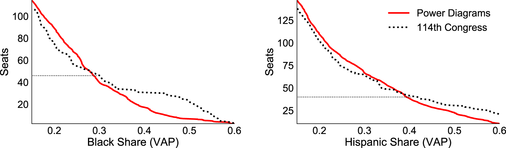
Armed with a population of maps, I aggregate the ethnic and racial composition of census tracts to calculate the Black and Hispanic fraction of each simulated district as I had previously done for the precinct-level votes. In Figure 4, I present the number of seats (actual and simulated) where the Black or Hispanic share of the voting age population (VAP) exceeds a given threshold. This exercise is grounded on the premise that the fraction of a district’s VAP belonging to a racial or ethnic majority is the key determinant in its electing a minority representative. The vertical distance between the dashed and solid lines gives a flavor for the change in minority representation from moving from the status quo to power-diagram-based districting if a single threshold triggered minority representation. The lines intersect in both panels. This suggests that if a high minority share were required to elect a minority representative, the currently enacted plans would result in higher minority representation than the power-diagram maps. Conversely, if a low minority share were required, the power-diagram maps could result in higher minority representation. Unlike the party share, where 50% is clearly the relevant threshold, there is no axiomatic level of minority presence for a minority candidate to be elected.
Presented are the number of districts whose population exceeds the shown thresholds of Black or Hispanic voting age population (VAP). For example, there are 74 districts whose population is at least 20% Black and 45 districts whose population is at least 30% Black. The composition of the 115th Congress, with 46 Black and 40 Hispanic lawmakers, is represented by the thin horizontal lines.

Acknowledging the complexity involved in measuring such a threshold and recognizing that using a single value countrywide is a gross simplification, I offer two simple approaches. The first is to identify the value of the VAP fraction  $f$ such that the number of constituencies with minority share greater than or equal to
 $f$ is matched by the number of minority representatives actually elected in the 115th Congress. At this level, each district with a larger minority share that does not elect a minority representative is compensated by another district with a lower share that does elect one. This is illustrated by a thin horizontal line in Figure 4. There were 40 Hispanic and 46 Black representatives in the 115th Congress,Footnote 5 which translates into fractions of 30% for Blacks and 41% for Hispanics.
Alternatively, Cameron, Epstein, and O’Halloran (Reference Cameron, Epstein and O’Halloran1996, Reference Epstein and O’Halloran1999) famously evaluated a probit model with the minority share of the VAP as the independent variable and an indicator for a minority representative as the dependent variable. Taking the simplest possible model with minority share  $x$, minority representation
 $r$, intercept
 $\unicode[STIX]{x1D6FC}$, and slope
 $\unicode[STIX]{x1D6FD}$, I fit the normal ogive
 $r=\unicode[STIX]{x1D6F7}(\unicode[STIX]{x1D6FD}x+\unicode[STIX]{x1D6FC})$. This simple approach ignores the interplay between Black and Hispanic populations and the role of primaries in determining the (Democratic) candidate (Lublin Reference Lublin1999; Lublin et al. Reference Lublin, Brunell, Grofman and Handley2009), and it is also markedly coarser than the local, ecological inference approach usually adopted in litigation. But the intent here is also very different: to evaluate the impact of a national change for which voting data are unavailable. In the 115th Congress, the 50% crossing point for this model is 35% for Blacks and 52% for Hispanics.
Intuitively, these thresholds correspond to a sizable majority of the majority party. The thresholds are higher for Hispanic districts due to higher eligibility and turnout among Blacks than Hispanics. Using the first approach to the threshold, the enacted and compactness-based maps produce an almost equal number of minority seats in the region of interest. To interpret the probit models, one must take the sum over districts of the probabilities of electing a minority. Doing this for the actual districts yields 46.0 Black and 40.0 Hispanic representatives compared to the true values of 46 and 40. The same sum of probabilities with the simulated maps yields 42.1 Black and 37.0 Hispanic representatives. According to the probit, a pure power-diagram approach would then lead to a 8% reduction in Black representation and a 7% reduction in Hispanic representation.
In practice, however, VRA compliance means that real districts constructed with a high minority share also typically have a partisan composition favorable to minority candidates. The power-diagram generation does not fine-tune this correlation, and power-diagram districts may, therefore, require a higher raw minority VAP fraction to elect a minority candidate. This caveat implies that the estimates of minority representation under power-diagram districts are likely inflated.
This said, in the past several Congresses, growth in minority representation has outpaced growth in the minority share of the population. This suggests that the “threshold” for minority representatives is falling. This point is reinforced by an earlier work by Grofman, Handley, and Lublin (Reference Grofman, Handley and Lublin2001). To the left of the intersections between curves of the enacted and simulated maps in Figure 4, the simulated maps yield higher minority fractions. If the threshold continues to fall, the minority representation under a compactness-based approach may exceed that from the current patchwork of judgment-based law.
Further, it is worth noting that the machinery already described provides the means for sidestepping the potential reductions in minority representation apparent in this analysis. One could include minority representation in the objective function or preferentially select maps with better minority prospects from the sets of automatically generated compactness-based districts. The latter approach is demonstrated in Appendix F.
6 Conclusions and Future Work
This paper has presented C4, a credible automated districting software that implements many compactness definitions and districting algorithms from the previous literature. This software facilitates quantitative, outcome-based discussion of districting objectives. Past compendia of compactness measures have not systematically implemented the proposed definitions in automated procedures and have, therefore, not been able to contrast the implications of the proposals.
Using this software, I have generated populations of contiguous and equipopulous maps for a number of states, optimized for each compactness measure and algorithm. Aggregating votes from presidential elections into the simulated districts, I have projected the “winner” of each district in each election. I have thus transformed the populations of maps into distributions of vote shares for seats and seat shares for states. The party vote shares across seats and elections reflect the political geography of the states; their distributions are remarkably consistent across methods, for each state. In particular, there is a good agreement in the integrals of vote shares above and below 0.5 (seat shares for the two parties) as well as between 0.475 and 0.525 (number of competitive seats). This consistency between methods suggests that the “unintentional gerrymandering” effect established by Chen and Rodden is quite robust to the specific, geometric definition of compactness. Using power diagrams to simulate hundreds of maps for every state in the country, I find that a purely compactness-based approach would result in small but noticeable reductions in minority representation.
This work offers a new strategy for evaluating the impacts of formal objectives for legislative districts, in the context of congressional action on gerrymandering in the United States. It could be extended by incorporating alternative initialization strategies including graph theoretic approaches and hierarchical partitioning or adding algorithms and compactness definitions. Studies like those of Chou et al. (Reference Chou, Kimbrough, Murphy, Sullivan-Fedock and Woodard2014) and Kaufman, King, and Komisarchik (Reference Kaufman, King and Komisarchik2017) that elicit human feedback on which measures yield the most appealing solutions could also be informative. Figure 3 shows that different objectives generate different shapes, and one can imagine ranking objective measures according to their subjective performance. Given the interest in protecting communities of interest and political subdivisions, it is worth formalizing and implementing objective functions to encode these adjacencies and other “normative” goals (minority representation, competitive districts, etc.). Such measures could then supplement or replace the spatial terms in the objective function, as illustrated in Appendix E.
Since the balance of this document has suggested that the various definitions of compactness are similar in their effects on representation, it is natural to ask which one to use. Power diagrams are a strong candidate. They converge quickly and reliably and result in clean, convex polygons—which is generally desirable but sometimes results in split cities (see Figure 3). Fryer and Holden (Reference Fryer and Holden2011) showed that power diagrams minimize the average interpersonal distance squared of co-constituents in the state. It is a nontrivial benefit that this distance is easy to comprehend. The interpersonal distance is also a good proxy for the other compactness measures. A PCA of the compactness measures of historic districts yields a first component that is correlated at  $\unicode[STIX]{x1D70C}=0.95$ with the interpersonal distance (Appendix I). On the other hand, power diagrams are implemented as a stand-alone algorithm and do not integrate as well with other objectives.
After selecting a measure, how compact should the districts in a map be? This paper has considered the behavior at convergence—maximal compactness—with no latitude left to the states. Critics might protest that this strategy imperils other traditional principles, like respect for political subdivisions or communities of interest. But that is not so: those objectives can be formalized and included in the optimization (Appendix E). As described in the context of minority representation (and demonstrated in Appendix F), one could also select plans from the distribution that satisfy some other objective. The algorithms presented here maximize compactness locally and not globally, so one might simply choose the most compact map. Strict maximization has the strong appeal of transparency. It is bundled with the immense but worthwhile challenge of formalizing and forging consent over objectives for democratic representation. If a looser standard were imposed by Congress, the appropriate analysis of impacts would shift to how effectively the standard constrained partisan cartographers. The present work has treated statewide compactness as the average (or sum) over districts, but more-nuanced criteria could be defined. The software developed could be extended and applied to each of these analyses.
Outright maximization also offers important preventative effect. The “bright line” of the Supreme Court’s “one-person, one-vote” standard (Gray v. Sanders 372 U.S. 368, 1963) virtually eliminated malapportioned districts. The justices long sought a similarly “precise rationale” for adjudicating partisan gerrymandering and have finally called off the search. Congress has the power to provide that rationale, as it did to protect minority voting rights. But the VRA’s history also highlights the challenges of nuance. The “Senate Factors” used to identify discriminatory election laws have forced the justices to exercise their gut judgment over the “totality of circumstances,” case by case. This conceptual obscurity has done little to dampen legislators’ appetites; the successes of the VRA have been achieved only through (or despite) relentless litigation. North Carolina’s 12th district has reached the Supreme Court on seven occasions since the 1992 redistricting: Shaw v. Reno (1993), Shaw v. Hunt (1996), Hunt v. Cromartie (1999), Easley v. Cromartie (2001), Cooper v. Harris (2017), and Rucho v. Common Cause (in both 2018 and 2019). With the VRA weakened by the Shelby County decision, preventative measures are needed to ensure minority voting rights. Strict, centralized maximization would deliver uniform districts more efficiently than nuanced criteria.
Of course, a new Apportionment Act is hardly the only proposed solution to political gerrymandering, nor is it the only one hinging on a clearer definition of compactness. As already noted, states can implement compactness requirements, and these may provide the footing for successful legal challenges. When the Pennsylvania Supreme Court determined in 2018 that a districting plan violated the state’s constitution, it struck down the plan and the US Supreme Court denied a petition to stay that ruling. In most of the developed world, redistricting is performed by independent commissions (Stephanopoulos Reference Stephanopoulos2013). These commissions must be charged with their objectives; should compactness rank among them, a single definition would provide clarity and consistency to the process. The present work has suggested that a choice among definitions need not be politics in disguise.
The Supreme Court’s long search for a “clear and manageable standard” for adjudicating partisan gerrymanders has come to an end with Rucho v. Common Cause. Reformers must now look elsewhere. It is has been an explicit aim of this paper to direct attention at the Federal level toward the constitutionally sanctioned, legislative pathways. Congress has a history of exercising this power. To revive and enrich debate over districting objectives, this paper has offered credible software and methods for evaluating and contrasting their practical impacts. Automated generation of compact districts is not the only solution to gerrymandering, and it is perhaps not a complete one. I contend, however, that optimization of explicit objectives is likely to be a useful tool for any solution—legislative or otherwise. A quantitative understanding of the implications of formal districting objectives is critical to both research and reform. I look forward to the continued refinement of algorithms and explicit objectives, for compactness and other districting aims.
Data Availability Statement
The replication materials for this paper can be found at Saxon (Reference Saxon2019).
Acknowledgements
I would like to thank Dan Black, Luc Anselin, Julia Koschinsky, Tom Coleman, Scott Ashworth, Wendy Wong, Gary King, Jonathan Rodden, Marc Farinella, Marc Elias, Ben Ginsberg, Harry Hirsch, the journal’s editor Jeff Gill, and four anonymous reviewers for valuable feedback on this project.
Supplementary Material
For supplementary material accompanying this paper, please visit https://doi.org/10.1017/pan.2019.45.