1 Introduction
Coastal erosion, a threat to coastal communities and life, is accelerating because climate change has resulted in more frequent and stronger storms (cf. Emanuel Reference Emanuel2005; Webster et al. Reference Webster, Holland, Curry and Chang2005). The Outer Banks of North Carolina are just one example of the areas that are very sensitive to storm conditions and that have sustained extensive property damage (Inman & Dolan Reference Inman and Dolan1989). The use of massive breakwaters as a means to mitigate storms of increasing severity remains the most common option despite well-known imperfections: breakwaters adversely alter the coastal environment, require strong and costly foundations, need frequent maintenance due to cyclic load of the waves as well as liquefaction of the top part and cause seabed soil subsidence at their foot besides potentially interfering with navigation.
In the 1980s, a promising alternative for coastal protection was put forward using a series of small man-made seabed-mounted corrugations to reflect the incident waves. The idea originated from the work of Davies (Reference Davies1982) who first studied the resonant interaction between free propagating surface waves and seabed undulations whose wavelengths are in a 2 : 1 ratio. The phenomenon is sometimes referred to as Bragg reflection or resonance due to its similarity with the selected reflection of X-rays from the surface of a crystal in solid state physics (see e.g. Pinsker Reference Pinsker1978). The strong reflection of water waves by seabed bars was shortly after investigated experimentally (cf. Heathershaw Reference Heathershaw1982; Davies & Heathershaw Reference Davies and Heathershaw1984) as well as theoretically (see Mitra & Greenberg Reference Mitra and Greenberg1984; Mei Reference Mei1985; Kirby Reference Kirby1986) and was observed in Cape Cod Bay (MA) where shore-parallel sandbars form naturally (Elgar, Raubenheimer & Herbers Reference Elgar, Raubenheimer and Herbers2003).
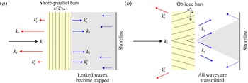
The idea of using longshore seabed-mounted bars for shore protection has been extensively studied theoretically, computationally and experimentally to understand its effectiveness and limitations (e.g. Bailard, DeVries & Kirby Reference Bailard, DeVries and Kirby1992). A number of issues, including for instance the formation of scours, were apparent during field experiments (Bailard et al. Reference Bailard, DeVries, Kirby and Guza1991), but it was an analytical investigation of the effect of beach reflection on the partially standing-wave pattern atop the corrugations which finally discredited the idea. Indeed, in agreement with earlier investigations of Kirby & Anton (Reference Kirby and Anton1991) and O’Hare & Davies (Reference O’Hare and Davies1993), Yu & Mei (Reference Yu and Mei2000) demonstrated that there can be a shoreward increase of wave amplitude when the shoreline reflection is sufficiently large. The Bragg-scattered shore-reflected waves and transmitted waves can be in a specific phase relationship depending on the distance between the shoreline and the patch of seabed bars, leading to constructive interference and amplification of waves (and not the expected reduction) at the coast (cf. figure 1 a). The erosion of both natural sandbars and beaches being inevitable, shore protection by Bragg reflection was subsequently deemed unreliable. The effect of reflective boundaries on Bragg resonance is now known to be of significant importance and interest in ocean engineering applications: it can lead to exponentially varying standing-wave patterns in wave tanks (Howard & Yu Reference Howard and Yu2007; Weidman et al. Reference Weidman, Herczynski, Yu and Howard2015) and is at the basis of the Fabry–Perot resonance mechanism reported in the context of water waves (see Couston et al. Reference Couston, Guo, Chamanzar and Alam2015).
Schematics of shore protection by (a) Bragg reflection and (b) Bragg deflection. The grey shaded area downstream of the corrugations represents the protected wake. (a) Most of the energy of an incident wave
 $k_{i}$
, that arrives normal to a patch of longshore seabed bars, is reflected back (
 $k_{r}$
). Nevertheless, a small part of the incident energy is still transmitted through the patch (
 $k_{t}$
). The waves
 $k_{t}$
, after reflecting back from the shoreline (dotted arrows), are reflected strongly by the patch (
 $k_{t}^{r}$
) with a small part transmitted back to the open ocean (
 $k_{t}^{t}$
). The process repeats as the
 $k_{t}^{r}$
wave reflected by the shoreline arrives again at the bars. Significant wave amplification can result from constructive wave interference between the trapped waves (i.e.
 $k_{t},k_{t}^{r},k_{t}^{rr},\ldots$
) depending on the distance between the patch and the shoreline (see Yu & Mei Reference Yu and Mei2000). (b) With oblique seabed bars, the incident wave
 $k_{i}$
is fully transmitted but also deflected to the sides in the downstream (
 $k_{t}$
). The
 $k_{t}$
waves are then reflected by the shoreline and cross back over the corrugated patch toward the open ocean (
 $k_{t}^{t}$
).

The resonance condition discovered by Davies (Reference Davies1982) for one horizontal dimension is a special case of the complete set of Bragg resonance conditions that can be obtained by regular perturbation of the three-dimensional potential flow equations for small corrugations (Liu & Yue Reference Liu and Yue1998). At each order of the perturbation expansion, a set of resonated waves are obtained from the bottom boundary condition in which the seabed harmonics interact with the lower-order wave solutions. The first-order variations of the incident waves at or near resonance can then be obtained using the method of multiple scales (e.g. Naciri & Mei Reference Naciri and Mei1988). For wave frequencies significantly different from the Bragg frequency, or in the presence of large-amplitude bottom corrugations, higher-order or exact theories such as Floquet theory are necessary to accurately predict solutions far from resonance, and to include evanescent modes and higher-order wave–bottom interactions (cf. e.g. exact linear theory of Yu & Howard Reference Yu and Howard2012, and references therein).
In cases where closed-form solutions cannot be obtained, a wide range of numerical models are available to study water-wave scattering by seabed topographies. These include the extended versions of the mild-slope equations (e.g. Kirby Reference Kirby1986; Porter & Staziker Reference Porter and Staziker1995), the coupled-mode approach (Athanassoulis & Belibassakis Reference Athanassoulis and Belibassakis1999; Belibassakis, Athanassoulis & Gerostathis Reference Belibassakis, Athanassoulis and Gerostathis2001), the integral matching/discretized bottom method (O’Hare & Davies Reference O’Hare and Davies1992; Seo Reference Seo2014), the fully nonlinear Boussinesq equation adjusted for rapid bottom undulations (see Madsen, Fuhrman & Wang Reference Madsen, Fuhrman and Wang2006) and the high-order spectral method (e.g. Dommermuth & Yue Reference Dommermuth and Yue1987). Numerical investigations of Bragg scattering have helped explain several discrepancies between theory and experiments, including: the difference between the observed and predicted class II Bragg resonance frequency due to evanescent modes (Guazzelli, Rey & Belzons Reference Guazzelli, Rey and Belzons1992) and the resonant frequency downshift/upshift for the subharmonic/superharmonic class III Bragg condition due to high-order nonlinearity (Madsen et al. Reference Madsen, Fuhrman and Wang2006).
Here we consider an arrangement of corrugations that can deflect, rather than reflect, shore-normal incident waves to the shore-parallel direction. We call this resonance mechanism Bragg deflection, to emphasize the contrast with Bragg reflection (since for the former the angle between the incident and resonated waves is less than or equal to
 $90^{\circ }$
). The proposed patch of corrugations, designed to be potentially useful for shore protection, has a plane of symmetry, aligned with the direction of incident wave propagation, such that the incident wave energy gets diverted in the downstream to the sides of a protected wake (see figure 1
b). One key advantage of the protection offered in the wake of such topography is that the protection efficiency is unaffected by coastal reflections. Waves reflected from the shoreline (either curved or straight) may be deflected by the patch but ultimately propagate back to the open ocean (
 $k_{t}^{t}$
waves in figure 1
b).
This manuscript considers the analysis of the Bragg deflection mechanism as a means of shore protection, and is organized as follows. The formulation of the problem, governing equations and Bragg resonance conditions are presented in § 2. In § 3, we investigate the protection provided by a monochromatic patch and show its limitations for cases where the deflection angle is large. The advantages of a bi-chromatic patch are then demonstrated analytically in § 4, using multiple-scale analysis. In § 5, we validate the multiple-scale results by direct simulation, and analyse the effect of detuning and perpendicular deflection. Finally, concluding remarks are drawn in § 6.
2 Problem formulation and resonance conditions
Consider the propagation of small-amplitude waves on the surface of an incompressible, homogeneous and inviscid fluid of mean water depth
 $h$
. We define a Cartesian coordinate system
 $(x,y,z)$
with the
 $x$
and
 $y$
axes lying on the mean free surface (we note
 $\hat{x}$
and
 ${\hat{y}}$
the corresponding unit vectors) and
 $z$
axis positive upward. Assuming irrotationality, the velocity vector
 $\boldsymbol{v}$
is written as
 $\boldsymbol{v}=\unicode[STIX]{x1D735}\unicode[STIX]{x1D6F7}$
where
 $\unicode[STIX]{x1D6F7}$
is the velocity potential. The velocity potential must satisfy the (linearized) potential flow equations
 $$\begin{eqnarray}\displaystyle & \unicode[STIX]{x1D6FB}^{2}\unicode[STIX]{x1D6F7}=0,\quad -h+\unicode[STIX]{x1D701}(x,y)\leqslant z\leqslant 0, & \displaystyle\end{eqnarray}$$
 $$\begin{eqnarray}\displaystyle & \unicode[STIX]{x1D6F7}_{tt}+g\unicode[STIX]{x1D6F7}_{z}=0,\quad z=0, & \displaystyle\end{eqnarray}$$
 $$\begin{eqnarray}\displaystyle & \unicode[STIX]{x1D6F7}_{z}=(-\unicode[STIX]{x1D735}_{h}h+\unicode[STIX]{x1D735}_{h}\unicode[STIX]{x1D701})\boldsymbol{\cdot }\unicode[STIX]{x1D735}_{h}\unicode[STIX]{x1D6F7},\quad z=-h+\unicode[STIX]{x1D701}(x,y), & \displaystyle\end{eqnarray}$$
 $g$
is the gravitational acceleration and
 $\unicode[STIX]{x1D735}_{h}=(\unicode[STIX]{x2202}_{x},\unicode[STIX]{x2202}_{y})$
is the horizontal gradient operator;
 $\unicode[STIX]{x1D701}(x,y)$
is the height of the small bottom corrugations measured from the mean seabed depth
 $z=-h$
. The free-surface elevation
 $\unicode[STIX]{x1D702}(x,y,t)$
is obtained from the linearized unsteady Bernoulli’s equation written on the free surface, i.e.
 $\unicode[STIX]{x1D702}=-\unicode[STIX]{x1D6F7}_{t}(z=0)/g$
. Under the assumption of small seabed corrugation slopes, i.e.
 $\unicode[STIX]{x1D735}_{h}\unicode[STIX]{x1D701}\sim O(\unicode[STIX]{x1D716})$
, where
 $\unicode[STIX]{x1D716}\ll 1$
is a small parameter, a first-order solution
 $\unicode[STIX]{x1D719}^{(1)}$
can be obtained from (2.1) by setting
 $\unicode[STIX]{x1D701}\equiv 0$
in (2.1c
). In this case the regular perturbation method predicts that an incident wave is unaffected at leading order by the presence of small seabed corrugations (see e.g. Liu et al.
Reference Liu, Yeh, Lin, Chang and Cho1998), and takes the general form
 $$\begin{eqnarray}\unicode[STIX]{x1D719}^{(1)}=\frac{A^{(1)}}{2}\frac{g}{\unicode[STIX]{x1D714}}\frac{\cosh [k(z+h)]}{\cosh (kh)}\text{e}^{\text{i}(\boldsymbol{k}\boldsymbol{\cdot }\boldsymbol{x}-\unicode[STIX]{x1D714}t)}+\text{c.c.},\end{eqnarray}$$
where
 $A^{(1)}$
is the wave amplitude and c.c. stands for complex conjugate. The wave frequency
 $\unicode[STIX]{x1D714}$
and wavenumber vector
 $\boldsymbol{k}$
are related through the dispersion relation
 $$\begin{eqnarray}{\mathcal{D}}(\unicode[STIX]{x1D714};k=|\boldsymbol{k}|)\equiv \unicode[STIX]{x1D714}^{2}-gk\tanh (kh)=0.\end{eqnarray}$$
As is well known, however, there can be a (Bragg) resonance between the incident waves and the corrugations such that a new wave
 $\boldsymbol{k}_{\boldsymbol{r}}$
is generated, which may have an amplitude as large as that of the incident wave. The resonance occurs at second order when the seabed component has wavenumber
 $\boldsymbol{k}_{b}$
such that
 $$\begin{eqnarray}{\mathcal{D}}(\unicode[STIX]{x1D714},|\boldsymbol{k}_{\boldsymbol{r}}|)=0,\quad \boldsymbol{k}_{\boldsymbol{r}}=\boldsymbol{k}\pm \boldsymbol{k}_{b},\end{eqnarray}$$
in which case the resonance is called class I (Liu et al.
Reference Liu, Yeh, Lin, Chang and Cho1998). The new wave must then be included at leading order, and the evolution of the incident and resonated wave amplitudes, also known as wave envelopes, can be obtained from multiple-scale analysis (e.g. Mei Reference Mei1985). When the bottom corrugations are multi-modal, the resonance can occur at a higher order as a result of the combined effect of two (or more) distinct bottom components. The resonance condition for two bottom components
 $\boldsymbol{k}_{b_{1}}$
and
 $\boldsymbol{k}_{b_{2}}$
reads
 $$\begin{eqnarray}{\mathcal{D}}(\unicode[STIX]{x1D714},|\boldsymbol{k}_{\boldsymbol{r}}|)=0,\quad \boldsymbol{k}_{\boldsymbol{r}}=\boldsymbol{k}\pm \boldsymbol{k}_{b_{1}}\pm \boldsymbol{k}_{b_{2}},\end{eqnarray}$$
and has been coined class II Bragg resonance when neither
 $\boldsymbol{k}_{b_{1}}$
or
 $\boldsymbol{k}_{b_{2}}$
satisfy (2.4).
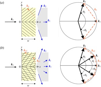
Here, we will explore the possibility to protect the shore by diverting, rather than by reflecting, the incident waves away from a protected area. We will first consider the classical oblique class I Bragg resonance, i.e. with (oblique) monochromatic seabed bars distributed in two adjacent patches symmetric with respect to
 $y=0$
, such that the incident waves are deflected toward
 $y=\pm \infty$
(cf. figure 2
a). It is, nevertheless, known that class I resonance is very weak for large deflection angles (i.e. for
 $\unicode[STIX]{x1D703}_{2}\rightarrow \unicode[STIX]{x03C0}/2$
, cf. figure 2
a), and is degenerate at
 $\unicode[STIX]{x1D703}_{2}=\unicode[STIX]{x03C0}/2$
. As we will show in this manuscript, it is therefore advantageous, in order to divert normally incident waves to the shore-parallel direction, to consider a superposition of two sets of oblique seabed bars, hence making the patch bi-chromatic (figure 2
b). In order for the transfer of energy from the incident
 $\boldsymbol{k}_{1}$
wave to the target
 $\boldsymbol{k}_{2}$
wave to be efficiently mediated by the transitional
 $\boldsymbol{k}_{t}$
wave, we will consider that
 $\boldsymbol{k}_{1}$
and
 $\boldsymbol{k}_{b_{1}}$
satisfy a class I Bragg resonance condition, i.e. (2.4). The proposed superposition of corrugations thus involves two corrugation modes, but all interactions happen at second order (in contrast to class II Bragg resonance that happens at the third order), such that, extending the nomenclature of Liu et al. (Reference Liu, Yeh, Lin, Chang and Cho1998), we will refer to this scenario as a class I
 $_{2}$
Bragg resonance condition.
Before proceeding to the derivation of the multiple-scale solutions, we would like to emphasize that here we are looking at a wave–bottom interaction problem with forward scattering. This is a very different situation from the classical Bragg reflection problem in which the resonated waves are back scattered, i.e. such that they propagate in a direction opposite to that of the incident waves. Here, in the case of forward scattering, all waves propagate in the same principal direction (i.e. in the positive
 $x$
direction, cf. figure 2). This is the reason why shore-reflected waves cannot be trapped (since they will be forward scattered toward the open ocean), but also it is the reason why Bragg deflection is not accumulative, contrary to the classical Bragg reflection: here, adding more seabed bars to the patch will not necessarily lead to additional scattering. This will be shown in details in the next two sections.
Schematics and Bragg resonance conditions for the deflection of
 $\boldsymbol{k}_{1}=k_{1}\hat{x}$
waves (with frequency
 $\unicode[STIX]{x1D714}$
) into
 $\boldsymbol{k}_{2}\;(=\boldsymbol{k}_{\boldsymbol{r}})$
waves by (a) a monochromatic patch through class I Bragg resonance, i.e. when
 ${\mathcal{D}}(\unicode[STIX]{x1D714},|\boldsymbol{k}_{2}|)=0$
where
 $\boldsymbol{k}_{2}=\boldsymbol{k}_{1}+\boldsymbol{k}_{b}$
(cf. (2.4)), and (b) a bi-chromatic patch through class I
 $_{2}$
Bragg resonance, i.e. when
 ${\mathcal{D}}(\unicode[STIX]{x1D714},|\boldsymbol{k}_{t}|)={\mathcal{D}}(\unicode[STIX]{x1D714},|\boldsymbol{k}_{2}|)=0$
where
 $\boldsymbol{k}_{t}=\boldsymbol{k}_{1}+\boldsymbol{k}_{b_{1}}$
and
 $\boldsymbol{k}_{2}=\boldsymbol{k}_{t}+\boldsymbol{k}_{b_{2}}$
(cf. (2.4) and (2.5)). The oblique parallel solid lines in the left figures represent the seabed bar crests whose corresponding wavenumbers are denoted by
 $\boldsymbol{k}_{b}$
for the monochromatic patch, and by
 $\boldsymbol{k}_{b_{1}}$
and
 $\boldsymbol{k}_{b_{2}}$
for the bi-chromatic patch. The problem is symmetric with respect to the
 $y=0$
plane such that significant wave energy reduction is expected in the shaded wake downstream of each patch. Note that all wavenumbers correspond to leading-order wave modes and therefore the superscripts
 $^{(1)}$
in (2.2) have been dropped.

3 Class I Bragg deflection for shore protection
Let us first consider a monochromatic patch with a plane of symmetry at
 $y=0$
, such that shore-normal incident waves are deflected to the sides of the
 $x$
axis by a set of oblique seabed bars (figure 2
a). The bottom corrugations are taken as
 $\unicode[STIX]{x1D701}(x,y)$
for
 $y>0$
and
 $\unicode[STIX]{x1D701}(x,-y)$
for
 $y<0$
, where
 $$\begin{eqnarray}\unicode[STIX]{x1D701}(x,y)=\left\{\begin{array}{@{}ll@{}}{\displaystyle \frac{d}{2}}(\text{e}^{\text{i}\boldsymbol{k}_{b}\boldsymbol{\cdot }\boldsymbol{x}}+\text{e}^{-\text{i}\boldsymbol{k}_{b}\boldsymbol{\cdot }\boldsymbol{x}}),\quad & 0<x<w,\\ 0,\quad & \text{otherwise},\end{array}\right.\end{eqnarray}$$
with
 $d$
the (real) positive corrugation amplitude and
 $w$
the patch width. Under class I Bragg resonance, i.e. when
 ${\mathcal{D}}(\unicode[STIX]{x1D714},|\boldsymbol{k}_{2}|)=0$
where
 $\boldsymbol{k}_{2}=\boldsymbol{k}_{1}+\boldsymbol{k}_{b}$
(cf. (2.4)), the incident and resonated wave amplitudes are of the same order, but their evolution is slow for small bottom corrugations, such that it can be decoupled from the fast variations of the carrier waves. Therefore, we consider a first-order velocity potential of the form
 $$\begin{eqnarray}\unicode[STIX]{x1D719}^{(1)}=\frac{g}{\unicode[STIX]{x1D714}}\frac{\cosh [k_{1}(z+h)]}{\cosh (k_{1}h)}\left[\frac{A_{1}(\bar{x},\bar{y},\bar{t})}{2}\text{e}^{\text{i}(\boldsymbol{k}_{1}\boldsymbol{\cdot }\boldsymbol{x}-\unicode[STIX]{x1D714}t)}+\frac{A_{2}(\bar{x},\bar{y},\bar{t})}{2}\text{e}^{\text{i}(\boldsymbol{k}_{2}\boldsymbol{\cdot }\boldsymbol{x}-\unicode[STIX]{x1D714}t)}\right]+\text{c.c.},\end{eqnarray}$$
where the incident (
 $A_{1}$
) and resonated (
 $A_{2}$
) wave amplitudes are functions of the slow space and time coordinates
 $(\bar{x},\bar{y},\bar{t})\sim \unicode[STIX]{x1D716}(x,y,t)$
with
 $\unicode[STIX]{x1D716}\ll 1$
, and governed by the so-called envelope equation (Mei Reference Mei1985)
 $$\begin{eqnarray}\displaystyle & \displaystyle \unicode[STIX]{x1D716}\frac{\unicode[STIX]{x2202}}{\unicode[STIX]{x2202}\bar{t}}A_{1}+\unicode[STIX]{x1D716}\boldsymbol{C}_{g_{1}}\boldsymbol{\cdot }\bar{\unicode[STIX]{x1D735}}A_{1}+\unicode[STIX]{x1D716}(\bar{\unicode[STIX]{x1D735}}\boldsymbol{\cdot }\boldsymbol{C}_{g_{1}})\frac{A_{1}}{2}=\text{i}A_{2}\unicode[STIX]{x1D6FA}_{c}, & \displaystyle\end{eqnarray}$$
 $$\begin{eqnarray}\displaystyle & \displaystyle \unicode[STIX]{x1D716}\frac{\unicode[STIX]{x2202}}{\unicode[STIX]{x2202}\bar{t}}A_{2}+\unicode[STIX]{x1D716}\boldsymbol{C}_{g_{2}}\boldsymbol{\cdot }\bar{\unicode[STIX]{x1D735}}A_{2}+\unicode[STIX]{x1D716}(\bar{\unicode[STIX]{x1D735}}\boldsymbol{\cdot }\boldsymbol{C}_{g_{2}})\frac{A_{2}}{2}=\text{i}A_{1}\unicode[STIX]{x1D6FA}_{c}, & \displaystyle\end{eqnarray}$$
 $\bar{\unicode[STIX]{x1D735}}=(\unicode[STIX]{x2202}/\unicode[STIX]{x2202}\bar{x},\unicode[STIX]{x2202}/\unicode[STIX]{x2202}\bar{y})$
and
 $$\begin{eqnarray}\unicode[STIX]{x1D6FA}_{c}=\frac{\unicode[STIX]{x1D714}d\boldsymbol{k}_{1}\boldsymbol{\cdot }\boldsymbol{k}_{2}}{2k_{1}\sinh (2k_{1}h)},\quad \boldsymbol{C}_{g_{j}}=\frac{\boldsymbol{k}_{j}\unicode[STIX]{x1D714}}{2k_{1}^{2}}\left[1+\frac{2k_{1}h}{\sinh (2k_{1}h)}\right]=\frac{\boldsymbol{k}_{j}}{k_{1}}C_{g}.\end{eqnarray}$$
Note that
 $\unicode[STIX]{x1D716}$
appears in front of all terms on the left-hand side of (3.3), but it is absent from the right-hand side. This is because the ripple amplitude is small, i.e.
 $k_{1}d\ll O(1)$
(as
 $O(k_{1})\sim O(k_{b})$
). The evolution of the incident and resonated waves can be shown based on (3.3) to be constrained by the energy preserving equation
 $$\begin{eqnarray}\frac{\unicode[STIX]{x2202}}{\unicode[STIX]{x2202}\bar{t}}\left(\frac{|A_{1}|^{2}}{2\unicode[STIX]{x1D714}}+\frac{|A_{2}|^{2}}{2\unicode[STIX]{x1D714}}\right)+\bar{\unicode[STIX]{x1D735}}\boldsymbol{\cdot }\left(\boldsymbol{C}_{g_{1}}\frac{|A_{1}|^{2}}{2\unicode[STIX]{x1D714}}+\boldsymbol{C}_{g_{2}}\frac{|A_{2}|^{2}}{2\unicode[STIX]{x1D714}}\right)=0,\end{eqnarray}$$
also known as the wave action equation. When appropriate, we will make use of the normalized amplitude variables
 $$\begin{eqnarray}a_{1}^{\ast }=\frac{|A_{1}|}{a_{0}},\quad a_{2}^{\ast }=\frac{|A_{2}|}{a_{0}}\sqrt{\cos \unicode[STIX]{x1D703}_{2}},\end{eqnarray}$$
(
 $a_{0}$
the incident wave amplitude) with which we can express the conservation of wave action more simply. Indeed, equation (3.5) reduces to
 $a_{1}^{\ast ^{2}}+a_{2}^{\ast ^{2}}=1$
for a patch infinitely long in the
 $y$
direction and at the steady state.
We solve (3.3) at steady state (i.e. assuming that the resonance condition is perfectly satisfied) in the upper half-plane (
 $x\geqslant 0$
,
 $y\geqslant 0$
). Since the problem is symmetric with respect to
 $y=0$
for normally and perfectly tuned incident waves, we then construct the solution in the lower half-plane by symmetry, i.e.
 $A_{1}$
and
 $A_{2}$
are even functions of
 $y$
. Because the system of (3.3) is typically not amenable to simple analytical treatment with variations in two horizontal dimensions (cf. e.g. the solution derived for a corner patch of parallel seabed bars in Mei, Hara & Naciri Reference Mei, Hara and Naciri1988), we numerically solve (3.3) in a steady state (i.e.
 $\unicode[STIX]{x2202}/\unicode[STIX]{x2202}\bar{t}\equiv 0$
) using an explicit finite-difference scheme. We use the Runge–Kutta fourth-order method for integration along the
 $x$
axis (spacing
 $\unicode[STIX]{x1D6FF}x$
between nodes), and a second-order central finite-difference scheme in
 $y$
(
 $\unicode[STIX]{x1D6FF}y$
).
The boundary conditions for
 $A_{1}$
and
 $A_{2}$
are obtained by requiring that the pressure and velocities be continuous at first order at the boundaries of the bar patch (cf. Naciri & Mei Reference Naciri and Mei1988): the condition turns out to be that the wave envelopes must be continuous as well, which is obtained because
 $A_{1}$
and
 $A_{2}$
are constants at first order, even though
 $\unicode[STIX]{x2202}A_{2}/\unicode[STIX]{x2202}\bar{x}$
may be non-zero at second order. Because the incident waves with wavenumber
 $\boldsymbol{k}_{1}=k_{1}\hat{x}$
are normally incident on the patch of seabed bars, we require that
 $A_{1}=a_{0}$
at the beginning of the patch
 $x=0$
where
 $a_{0}$
is the incident wave amplitude. This fulfils the boundary condition in
 $x$
for (3.3a
). For the resonated waves, which are forward-scattered waves, the boundary condition in
 $x$
is also enforced at
 $x=0$
such that
 $A_{2}(x=0)=0$
. In
 $y$
, the boundary condition is
 $A_{2}=0$
at
 $y=0$
due to the fact that the resonated wave amplitude is necessarily zero along the patch’s plane of symmetry (see figure 2
b); the
 $A_{2}$
waves are forward scattered and propagate in the
 $+y$
direction for the upper patch, and they are zero where their characteristic lines start. From (3.3b
), we then find that
 $A_{1}=a_{0}$
at
 $y=0$
. We note that the problem over the corrugated domain is well posed in the sense that we have two coupled first-order advection equations with characteristic lines supported by the group velocity vectors
 $\boldsymbol{C}_{g_{1}}$
and
 $\boldsymbol{C}_{g_{2}}$
going into the domain
 $\mathbb{R}^{+}\times \mathbb{R}^{+}$
. The boundary conditions at
 $x=0$
and
 $y=0$
are therefore necessary and sufficient to obtain a solution, as was the case for the similar problem of wave scattering by a corner bar field solved in Mei et al. (Reference Mei, Hara and Naciri1988). This is of course in contrast with the classical Bragg reflection problem, which requires a boundary condition at the beginning of the patch for the incident wave and a boundary condition at the end of the patch for the backward-scattered wave.
It should be noted that the condition
 $A_{1}=1$
along
 $y=0$
is not a boundary condition, but rather a consequence of the multiple-scale equation (3.3b
). In fact, no boundary conditions are required for
 $A_{1}$
in
 $y$
because the advection equation (3.3b
) has a characteristic line going in
 $x$
only. This is a limitation of the multiple-scale method, which neglects diffraction effects, as was already discussed in Mei et al. (Reference Mei, Hara and Naciri1988). At a boundary
 $y=y_{e}$
where
 $y=y_{e}$
is the end of the upper patch, we would find that
 $A_{1}$
is discontinuous:
 $A_{1}=1$
at
 $y=y_{e}+\unicode[STIX]{x1D716}_{y}$
(i.e. just outside of the patch) while
 $A_{1}$
is non-uniform at
 $y_{e}-\unicode[STIX]{x1D716}_{y}$
(i.e. over the patch), where
 $\unicode[STIX]{x1D716}_{y}$
is an arbitrary infinitesimally small parameter (
 $\unicode[STIX]{x1D716}_{y}\ll \unicode[STIX]{x1D706}_{1}$
). This implies that
 $\boldsymbol{k}_{1}$
waves just outside of the patch could influence the solution on the edge of the corrugated patch, an effect which can be modelled using the parabolic approximation that allows for slow variations (i.e. diffraction) of the envelope amplitudes perpendicularly to the waves’ direction of propagation (see e.g. Kirby Reference Kirby1986). Diffraction effects will be further discussed in § 5.1, but in brief are not investigated here. Again, this is a limitation of our model, but because diffraction effects should remain confined near the edge of the corrugated patch (and not contaminate the entire solution), they are not expected to have a major influence on the overall solution.
The forward scattering of waves with Bragg deflection is the reason why the solution obtained for the semi-infinite patch can be used as the solution for any finite-width patch: the solution obtained for
 $x\in [0,x_{e}]$
will be the same for a patch of width greater than
 $x_{e}$
but finite, or for a semi-infinite patch. The only difference will be that the envelope amplitudes outside of a finite-width patch will be constant outside of the patch, while they continue to change for the semi-infinite patch. Thus, it is clear that the problem of the semi-infinite patch is the most relevant problem to solve, since it provides us with a solution, which once truncated to a finite domain size, is in fact the solution obtained for a finite-width patch. This also holds for the extent of the patch in the
 $y$
direction. The solution obtained for the infinitely long patch (
 $-\infty <y<+\infty$
), once truncated, can be used as the solution for a patch of finite extent in
 $y$
, i.e.
 $-y_{e}<y<+y_{e}$
. Note that none of this is true for the problem of Bragg reflection, since in this case a longer patch (in
 $x$
) leads to more scattering due to the fact that Bragg reflection is an accumulative effect.
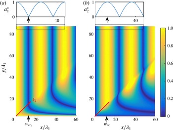
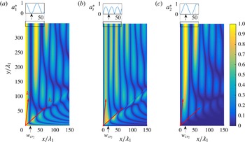
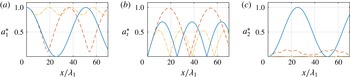
Normalized envelope amplitudes (a)
 $a_{1}^{\ast }$
and (b)
 $a_{2}^{\ast }$
(cf. (3.6)) as obtained from (3.3) with
 $\unicode[STIX]{x2202}/\unicode[STIX]{x2202}\bar{t}\equiv 0$
. The patch is semi-infinite, starting from
 $x=0$
, and the bottom corrugations are given by
 $\unicode[STIX]{x1D701}(x,y)$
for
 $y>0$
and by
 $\unicode[STIX]{x1D701}(x,-y)$
for
 $y<0$
(cf. (3.1) with
 $w=+\infty$
). The amplitude modulations far from the plane of symmetry (highlighted in the rectangles) are clearly the same as for the one-dimensional solution (shown by the solid lines in the top figures). We only show the amplitudes for
 $y>0$
since the problem is symmetric with respect to the
 $y=0$
axis. The small vertical arrows show the location of the critical patch width
 $w_{cr_{1}}$
(such that
 $a_{1}^{\ast }(x=w_{cr_{1}})=0$
far from
 $y=0$
), and the oblique arrows starting from the origin of each axis show the direction of propagation of the
 $\boldsymbol{k}_{2}$
waves. The physical parameters are
 $\unicode[STIX]{x1D703}_{2}=\unicode[STIX]{x03C0}/4$
,
 $k_{1}h=0.2$
,
 $d/h=0.1$
. The simulation parameters are
 $\unicode[STIX]{x1D6FF}x/\unicode[STIX]{x1D706}_{1}=0.05$
and
 $\unicode[STIX]{x1D6FF}y/\unicode[STIX]{x1D706}_{1}=0.2$
.

The variations of the wave amplitudes over a semi-infinite monochromatic patch (
 $x\geqslant 0$
) are shown in figure 3, with
 $\unicode[STIX]{x1D703}_{2}=\unicode[STIX]{x03C0}/4$
. Note, again, that we solve a semi-infinite patch problem, since as previously discussed, the solution for a finite-size patch is the same over the corrugations, i.e. for
 $x\leqslant x_{e}$
where
 $x_{e}$
is the end point of the finite-size patch. While the behaviour of the wave amplitudes is relatively complex near the patch’s plane of symmetry, the evolution becomes one-dimensional and periodic for
 $y/\unicode[STIX]{x1D706}_{1}\gg 1$
, which we will refer to as the far field. The one-dimensional behaviour of the solution can only be obtained in the region where both the incident and scattered waves co-exist from
 $x=0$
onward; this region is obtained for
 $y>x\cos \unicode[STIX]{x1D703}_{2}$
, i.e. above the
 $\boldsymbol{k}_{2}$
vector shown in figure 3. The condition
 $y>x\cos \unicode[STIX]{x1D703}_{2}$
shows that the far field is a function of
 $x$
: the longer the patch, the further away from the patch’s plane of symmetry we recover the one-dimensional solution. Assuming
 $\unicode[STIX]{x2202}/\unicode[STIX]{x2202}\bar{y}\equiv 0$
, the solution far from the patch’s plane of symmetry can thus be approximated by the solution of the one-dimensional problem, whose closed-form solution becomes
 $$\begin{eqnarray}\left(\begin{array}{@{}c@{}}A_{1}\\ A_{2}\end{array}\right)=a_{0}\left(\begin{array}{@{}c@{}}\cos K_{c}x\\ \displaystyle \frac{-\text{i}}{\sqrt{\cos \unicode[STIX]{x1D703}_{2}}}\sin K_{c}x\end{array}\right),\end{eqnarray}$$
where
 $$\begin{eqnarray}K_{c}=\unicode[STIX]{x1D6FA}_{c}/(C_{g}\sqrt{\cos \unicode[STIX]{x1D703}_{2}}).\end{eqnarray}$$
Because the
 $y$
-invariant solution (3.7) is oscillatory with period
 $2\unicode[STIX]{x03C0}/K_{c}$
, as can be seen in figure 3, the incident wave energy far from the plane of symmetry is fully transferred to the deflected wave mode (i.e.
 $A_{1}=a_{1}^{\ast }=0$
) at
 $x=w_{cr_{1}}=\unicode[STIX]{x03C0}/(2K_{c})$
. Therefore,
 $w_{cr_{1}}$
is the critical monochromatic patch width since it is the shortest width that minimizes the amplitude of the incident waves in the downstream and away from the patch’s plane of symmetry. At the end of a patch truncated at
 $x=w_{cr_{1}}$
, most of the incident wave energy is deflected sideways in the form of waves that make the angle
 $\unicode[STIX]{x1D703}_{2}$
with respect to the
 $x$
axis. Significant shore protection can thus be expected downstream of the patch, in a wake that looks like an isosceles triangle, with a vertex angle twice the angle
 $\unicode[STIX]{x1D703}_{2}$
of the Bragg resonated wave (see figure 2). It is remarked that class I Bragg resonance is degenerate at
 $\unicode[STIX]{x1D703}_{2}=\unicode[STIX]{x03C0}/2$
. It can be shown that
 $w_{cr_{1}}\rightarrow \infty$
when
 $\unicode[STIX]{x1D703}_{2}\rightarrow \unicode[STIX]{x03C0}/2$
, i.e. a monochromatic bar patch must be infinitely wide for large deflection angles. The decreased efficiency of energy transfer between the incident and deflected waves for deflection angles
 $\unicode[STIX]{x1D703}_{2}\sim \unicode[STIX]{x03C0}/2$
implies that a monochromatic patch cannot be used to protect large regions of a coast. This limitation is lifted in the next section as we show that a bi-chromatic patch, with the same total ripple amplitude as for the monochromatic patch, is very efficient at deflecting incident waves for all
 $\unicode[STIX]{x1D703}_{2}$
angles.
4 Class I
 $_{2}$
Bragg deflection for shore protection

Here we consider the case of a bi-chromatic patch for which the transfer of
 $\boldsymbol{k}_{1}$
wave energy to the
 $\boldsymbol{k}_{2}$
wave is mediated by a transitional Bragg resonated
 $\boldsymbol{k}_{t}$
wave (cf. figure 2
b). The key result of this section is that the critical bi-chromatic patch width
 $w_{cr_{2}}$
is much smaller than the critical monochromatic patch width
 $w_{cr_{1}}$
for large deflection angles
 $\unicode[STIX]{x1D703}_{2}$
. Based on the results for the monochromatic patch and in order to derive the critical patch width
 $w_{cr_{2}}$
, we first study the behaviour of the envelope amplitudes far from the patch’s plane of symmetry. We then solve the multiple-scale equations for the case of a patch with a plane of symmetry using the finite-difference scheme presented in § 3.
4.1 Closed-form solution far from the patch’s plane of symmetry
Here we derive the envelope equations for wave propagation over a bi-chromatic patch, i.e. with bottom corrugations of the form
 $$\begin{eqnarray}\unicode[STIX]{x1D701}=\frac{d_{1}}{2}(\text{e}^{\text{i}\boldsymbol{k}_{b_{1}}\boldsymbol{\cdot }\boldsymbol{ x}}+\text{e}^{-\text{i}\boldsymbol{k}_{b_{1}}\boldsymbol{\cdot }\boldsymbol{x}})+\frac{d_{2}}{2}(\text{e}^{\text{i}\boldsymbol{k}_{b_{2}}\boldsymbol{\cdot }\boldsymbol{ x}}+\text{e}^{-\text{i}\boldsymbol{k}_{b_{2}}\boldsymbol{\cdot }\boldsymbol{x}}),\end{eqnarray}$$
with
 $d_{1}$
and
 $d_{2}$
the (real) positive corrugation amplitudes. We assume that the incident wave number
 $\boldsymbol{k}_{1}$
satisfies both the class I and class II Bragg resonance conditions (which we refer to as class I
 $_{2}$
), i.e.
 ${\mathcal{D}}(\unicode[STIX]{x1D714},|\boldsymbol{k}_{t}|)={\mathcal{D}}(\unicode[STIX]{x1D714},|\boldsymbol{k}_{2}|)=0$
(cf. (2.4) and (2.5)), such that
 $\boldsymbol{k}_{t}=\boldsymbol{k}_{1}+\boldsymbol{k}_{b_{1}}$
and
 $\boldsymbol{k}_{2}=\boldsymbol{k}_{t}+\boldsymbol{k}_{b_{2}}$
are free propagating waves. Since the wave
 $\boldsymbol{k}_{t}$
is the first wave resonated, it can be shown using a regular perturbation method that initially the
 $\boldsymbol{k}_{t}$
wave amplitude increases linearly in time while the
 $\boldsymbol{k}_{2}$
wave growth is quadratic.
To obtain the multiple-scale equations for the bi-modal corrugation problem under the assumption of small bottom steepness, we consider a leading-order velocity potential of the form
 $$\begin{eqnarray}\unicode[STIX]{x1D719}^{(1)}=\frac{g}{\unicode[STIX]{x1D714}}\frac{\cosh [k_{1}(z+h)]}{\cosh (k_{1}h)}\left(\frac{A_{1}}{2}\text{e}^{\text{i}\boldsymbol{k}_{1}\boldsymbol{\cdot }\boldsymbol{ x}}+\frac{A_{t}}{2}\text{e}^{\text{i}\boldsymbol{k}_{t}\boldsymbol{\cdot }\boldsymbol{ x}}+\frac{A_{2}}{2}\text{e}^{\text{i}\boldsymbol{k}_{2}\boldsymbol{\cdot }\boldsymbol{ x}}\right)\text{e}^{-\text{i}\unicode[STIX]{x1D714}t}+\text{c.c.},\end{eqnarray}$$
where the envelope amplitudes
 $A_{1}$
,
 $A_{t}$
and
 $A_{2}$
are functions of the slow variables
 $(\bar{x},\bar{y},\bar{t})\sim \unicode[STIX]{x1D716}(x,y,t)$
. Similar to the monochromatic problem, we derive the evolutionary equations for the slowly varying amplitudes from the so-called compatibility condition, obtained upon inspection of the second-order problem in terms of the bottom steepness. The derivation is provided in Appendix I, and the final equations read
 $$\begin{eqnarray}\displaystyle & \displaystyle \unicode[STIX]{x1D716}\frac{\unicode[STIX]{x2202}}{\unicode[STIX]{x2202}\bar{t}}A_{1}+\boldsymbol{C}_{g_{1}}\boldsymbol{\cdot }\unicode[STIX]{x1D716}\bar{\unicode[STIX]{x1D735}}A_{1}+\frac{A_{1}}{2}\unicode[STIX]{x1D716}\bar{\unicode[STIX]{x1D735}}\boldsymbol{\cdot }\boldsymbol{C}_{g_{1}}=\text{i}A_{t}\unicode[STIX]{x1D6FA}_{1}, & \displaystyle\end{eqnarray}$$
 $$\begin{eqnarray}\displaystyle & \displaystyle \unicode[STIX]{x1D716}\frac{\unicode[STIX]{x2202}}{\unicode[STIX]{x2202}\bar{t}}A_{t}+\boldsymbol{C}_{g_{t}}\boldsymbol{\cdot }\unicode[STIX]{x1D716}\bar{\unicode[STIX]{x1D735}}A_{t}+\frac{A_{t}}{2}\unicode[STIX]{x1D716}\bar{\unicode[STIX]{x1D735}}\boldsymbol{\cdot }\boldsymbol{C}_{g_{t}}=\text{i}A_{1}\unicode[STIX]{x1D6FA}_{1}+\text{i}A_{2}\unicode[STIX]{x1D6FA}_{2}, & \displaystyle\end{eqnarray}$$
 $$\begin{eqnarray}\displaystyle & \displaystyle \unicode[STIX]{x1D716}\frac{\unicode[STIX]{x2202}}{\unicode[STIX]{x2202}\bar{t}}A_{2}+\boldsymbol{C}_{g_{2}}\boldsymbol{\cdot }\unicode[STIX]{x1D716}\bar{\unicode[STIX]{x1D735}}A_{2}+\frac{A_{2}}{2}\unicode[STIX]{x1D716}\bar{\unicode[STIX]{x1D735}}\boldsymbol{\cdot }\boldsymbol{C}_{g_{2}}=\text{i}A_{t}\unicode[STIX]{x1D6FA}_{2}, & \displaystyle\end{eqnarray}$$
 $\boldsymbol{C}_{g_{j}}$
(
 $j=1,t,2$
) is given by (3.4), and
 $$\begin{eqnarray}\unicode[STIX]{x1D6FA}_{1}=\frac{\unicode[STIX]{x1D714}d_{1}\boldsymbol{k}_{1}\boldsymbol{\cdot }\boldsymbol{k}_{t}}{2k_{1}\sinh 2k_{1}h},\quad \unicode[STIX]{x1D6FA}_{2}=\frac{\unicode[STIX]{x1D714}d_{2}\boldsymbol{k}_{t}\boldsymbol{\cdot }\boldsymbol{k}_{2}}{2k_{1}\sinh 2k_{1}h}.\end{eqnarray}$$
The governing equations (4.3) are valid for slow mean bottom variations, but for mathematical expediency, we will now assume that
 $h$
is constant (i.e. such that
 $\bar{\unicode[STIX]{x1D735}}\boldsymbol{\cdot }\boldsymbol{C}_{g_{1}}=\bar{\unicode[STIX]{x1D735}}\boldsymbol{\cdot }\boldsymbol{C}_{g_{t}}=\bar{\unicode[STIX]{x1D735}}\boldsymbol{\cdot }\boldsymbol{C}_{g_{2}}=0$
in (4.3)). The case of a slowly varying mean water depth, of particular interest near the coast where the beach is usually gently sloped (see e.g. Mei, Hara & Yu Reference Mei, Hara and Yu2001), does not change the qualitative behaviour of Bragg resonance and can be in fact estimated relatively simply. The wave–bottom interactions indeed remain resonant even when the mean depth is changing, as long as the Bragg condition, which changes as the depth increases or decreases, is satisfied everywhere locally. As a result, the Bragg resonance can be maintained by adjusting the corrugation wavelength to the local surface wavelength, which is what occurs naturally for sandbar formation on sloped beaches (see e.g. Dulou, Belzons & Rey Reference Dulou, Belzons and Rey2000). Doing this, it is expected that the efficiency of the Bragg reflection (or here deflection) of the total corrugated patch over the varying mean depth (say
 $h_{s}<h<h_{d}$
) is less than the efficiency obtained in the constant shallow water case (
 $h=h_{s}$
), but more than in the constant deep water case (
 $h=h_{d}$
) (cf. e.g. Alam Reference Alam2012a
).
The conservation of the wave action equation
 $$\begin{eqnarray}\frac{\unicode[STIX]{x2202}}{\unicode[STIX]{x2202}\bar{t}}\left(\frac{|A_{1}|^{2}}{2\unicode[STIX]{x1D714}}+\frac{|A_{t}|^{2}}{2\unicode[STIX]{x1D714}}+\frac{|A_{2}|^{2}}{2\unicode[STIX]{x1D714}}\right)+\bar{\unicode[STIX]{x1D735}}\boldsymbol{\cdot }\left(\boldsymbol{C}_{g_{1}}\frac{|A_{1}|^{2}}{2\unicode[STIX]{x1D714}}+\boldsymbol{C}_{g_{t}}\frac{|A_{t}|^{2}}{2\unicode[STIX]{x1D714}}+\boldsymbol{C}_{g_{2}}\frac{|A_{2}|^{2}}{2\unicode[STIX]{x1D714}}\right)=0,\end{eqnarray}$$
derived from (4.3), is the natural extension of (3.5) to the three-wave interaction problem. By defining the normalized transitional wave amplitude
 $a_{t}^{\ast }=|A_{t}|\sqrt{\cos \unicode[STIX]{x1D703}_{t}}/a_{0}$
, equation (4.5) reduces to
 $a_{1}^{\ast ^{2}}+a_{t}^{\ast ^{2}}+a_{2}^{\ast ^{2}}=1$
when
 $\unicode[STIX]{x2202}/\unicode[STIX]{x2202}\bar{t}\equiv \unicode[STIX]{x2202}/\unicode[STIX]{x2202}\bar{y}\equiv 0$
(cf. (3.6) for
 $a_{1,2}^{\ast }$
).
In the case of perfectly tuned waves far from the patch’s plane of symmetry, a closed-form solution can be derived at the steady state. Specifically, assuming
 $\unicode[STIX]{x2202}/\unicode[STIX]{x2202}\bar{t}\equiv \unicode[STIX]{x2202}/\unicode[STIX]{x2202}\bar{y}\equiv 0$
and enforcing the boundary conditions for the incident wave
 $A_{1}=a_{0}$
, and resonated waves
 $A_{t}=A_{2}=0$
(which all propagate in the
 $+x$
direction) at
 $x=0$
, we obtain the solution
 $$\begin{eqnarray}\left(\begin{array}{@{}c@{}}A_{1}\\ A_{t}\\ A_{2}\end{array}\right)=\frac{a_{0}K_{1}K_{2}}{K_{12}}\left(\begin{array}{@{}c@{}}K_{2}/K_{1}+K_{1}/K_{2}\cos K_{12}x\\ \text{i}K_{12}/K_{2}\sin K_{12}x\\ -1+\cos K_{12}x\end{array}\right),\end{eqnarray}$$
where
 $$\begin{eqnarray}K_{1}=\unicode[STIX]{x1D6FA}_{1}/(C_{g}\sqrt{\cos \unicode[STIX]{x1D703}_{t}}),\quad K_{2}=\unicode[STIX]{x1D6FA}_{2}/(C_{g}\sqrt{\cos \unicode[STIX]{x1D703}_{t}\cos \unicode[STIX]{x1D703}_{2}}),\quad K_{12}=\sqrt{K_{1}^{2}+K_{2}^{2}}.\end{eqnarray}$$
The envelope amplitudes (4.6) are oscillatory over the patch, but the initial
 $\boldsymbol{k}_{1}$
wave does not necessarily cede all its energy to the
 $\boldsymbol{k}_{t}$
or
 $\boldsymbol{k}_{2}$
waves. For
 $d_{2}\neq 0$
, the
 $\boldsymbol{k}_{1}$
wave amplitude reaches a minimum of
 $A_{1}=a_{0}(K_{2}^{2}-K_{1}^{2})/K_{12}$
at
 $x=\unicode[STIX]{x03C0}/K_{12}$
, which is zero if and only if
 $$\begin{eqnarray}K_{2}=K_{1}\quad \Leftrightarrow \quad d_{2}/d_{1}=\sqrt{\cos \unicode[STIX]{x1D703}_{2}}\frac{\cos \unicode[STIX]{x1D703}_{t}}{\cos (\unicode[STIX]{x1D703}_{2}-\unicode[STIX]{x1D703}_{t})},\end{eqnarray}$$
in which case
 $K_{12}$
reduces to
 $$\begin{eqnarray}K_{12}=\sqrt{2}K_{1}.\end{eqnarray}$$
Equation (4.8) describes the necessary balance between the efficiency of the
 $\boldsymbol{k}_{1}\leftrightarrow \boldsymbol{k}_{t}$
and
 $\boldsymbol{k}_{t}\leftrightarrow \boldsymbol{k}_{2}$
Bragg interactions to achieve a synchronous energy transfer from
 $\boldsymbol{k}_{1}$
to
 $\boldsymbol{k}_{2}$
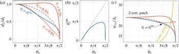
: if one of the deflection angles increases relative to the other, which diminishes the corresponding interaction efficiency, then the associated ripple amplitude should also increase in order to balance the effect. The condition (4.8) is illustrated in figure 4(a) where we show the ratio
 $d_{2}/d_{1}$
as a function of
 $\unicode[STIX]{x1D703}_{2}$
for four different transitional angles. Clearly
 $d_{2}/d_{1}$
decreases when
 $\unicode[STIX]{x1D703}_{t}$
increases since the
 $\boldsymbol{k}_{t}\leftrightarrow \boldsymbol{k}_{2}$
Bragg interaction becomes more effective with decreasing
 $\unicode[STIX]{x1D703}_{2}-\unicode[STIX]{x1D703}_{t}$
. The ratio
 $d_{2}/d_{1}$
also decreases almost monotonically with increasing
 $\unicode[STIX]{x1D703}_{2}$
since the
 $\boldsymbol{k}_{2}$
wave’s time spent over the patch, or, in other words, the number of wave–seabed interactions, scales with
 $\sqrt{1+\tan ^{2}\unicode[STIX]{x1D703}_{2}}$
. For instance, when
 $\boldsymbol{k}_{1}$
waves travel one unit distance in the
 $x$
direction,
 $\boldsymbol{k}_{2}$
waves only move by
 $\cos \unicode[STIX]{x1D703}_{2}$
in
 $x$
.
(a) Ratio of the corrugation amplitudes
 $d_{2}/d_{1}$
as a function of
 $\unicode[STIX]{x1D703}_{2}$
, such that full energy transfer is achieved between the
 $\boldsymbol{k}_{1}$
wave and the
 $\boldsymbol{k}_{2}$
wave at the end of a patch of width
 $w=w_{cr_{2}}=\unicode[STIX]{x03C0}/K_{12}$
(cf. (4.8)). The four different curves correspond to different transitional angles
 $\unicode[STIX]{x1D703}_{t}$
. (b) The unique optimal transitional angle
 $\unicode[STIX]{x1D703}_{t}^{opt}$
as a function of
 $\unicode[STIX]{x1D703}_{2}$
, which minimizes the critical patch width
 $w_{cr_{2}}$
for fixed total ripple amplitude
 $(d_{1}+d_{2})/h=0.12$
and normalized water depth
 $k_{1}h=0.2$
, and provided that (4.8) is satisfied. (c) Plot of the critical patch width
 $w_{cr_{2}}$
for bi-modal corrugations (2-corr. patch curves; corr. short for corrugation) for various transitional angles (same line-style notation as in figure 4
a). We also plot the critical patch width for a monochromatic patch
 $w_{cr_{1}}=\unicode[STIX]{x03C0}/(2K_{c})$
(1-corr. patch) for which the corrugation amplitude is
 $d/h=0.12$
(cf. (3.8)). The critical monochromatic patch width becomes rapidly much larger than the critical bi-chromatic patch width when
 $\unicode[STIX]{x1D703}_{2}\rightarrow \unicode[STIX]{x03C0}/2$
.

When (4.8) is satisfied, the energy carried by the
 $\boldsymbol{k}_{1}$
waves transfers to
 $\boldsymbol{k}_{2}$
waves after travelling the distance
 $w_{cr_{2}}=\unicode[STIX]{x03C0}/K_{12}$
, which we call the critical bi-chromatic patch width. For fixed
 $\unicode[STIX]{x1D703}_{2}$
and normalized total ripple amplitude
 $(d_{1}+d_{2})/h$
, the critical bi-chromatic patch width has a unique minimum at
 $\unicode[STIX]{x1D703}_{t}=\unicode[STIX]{x1D703}_{t}^{opt}$
, such that
 $\unicode[STIX]{x1D703}_{t}^{opt}$
maximizes
 $K_{12}$
as given by (4.9). Figure 4(b) shows the variations of
 $\unicode[STIX]{x1D703}_{t}^{opt}$
as a function of
 $\unicode[STIX]{x1D703}_{2}$
.
In practice,
 $\unicode[STIX]{x1D703}_{t}^{opt}$
can be approximated by
 $\unicode[STIX]{x1D703}_{2}/2$
because the critical patch widths for
 $\unicode[STIX]{x1D703}_{t}^{opt}$
and
 $\unicode[STIX]{x1D703}_{2}/2$
are nearly the same. This can be seen from the overlap of the
 $w_{cr_{2}}$
curve obtained for
 $\unicode[STIX]{x1D703}_{t}^{opt}$
with the dashed curve obtained for
 $\unicode[STIX]{x1D703}_{t}=\unicode[STIX]{x1D703}_{2}/2$
in figure 4(c). Figure 4(c) also shows the critical patch width
 $w_{cr_{1}}$
for a monochromatic patch. Interestingly,
 $w_{cr_{2}}$
is greater than
 $w_{cr_{1}}$
for relatively small deflection angles because we have assumed
 $d_{2}\neq 0$
in deriving (4.8). By setting
 $d_{2}=0$
, we get
 $w_{cr_{2}}=w_{cr_{1}}$
since both patches involve only one Bragg interaction. Since
 $w_{cr_{1}}=w_{cr_{2}}$
at
 $\unicode[STIX]{x1D703}_{2}\sim 11\unicode[STIX]{x03C0}/25$
for
 $\unicode[STIX]{x1D703}_{t}=\unicode[STIX]{x1D703}_{2}/2$
, as depicted in figure 4(c) (intersection of the dashed line with the 1-corr. curve, i.e. the curve obtained for a monochromatic patch; corr. short for corrugation), the bi-chromatic patch becomes significantly more efficient for shore protection when deflection angles satisfy
 $\unicode[STIX]{x1D703}_{2}>11\unicode[STIX]{x03C0}/25$
.
While the values predicted by the method of multiple scales for
 $d_{2}/d_{1}$
(see figure 4
a),
 $\unicode[STIX]{x1D703}_{t}^{opt}$
(figure 4
b), and
 $w_{cr_{2}}$
(figure 4
c) are valid for most
 $\unicode[STIX]{x1D703}_{2}$
, the trends in the limit of
 $\unicode[STIX]{x1D703}_{2}\rightarrow 0$
or
 $\unicode[STIX]{x1D703}_{2}\rightarrow \unicode[STIX]{x03C0}/2$
may be inaccurate. Indeed,
 $\unicode[STIX]{x1D703}_{2}\sim 0$
implies seabed bar crests almost parallel to
 $\boldsymbol{k}_{1}$
, which invalidates the multiple-scale assumption of a rapidly varying water depth in
 $x$
. The configuration
 $\unicode[STIX]{x1D703}_{t}\sim \unicode[STIX]{x1D703}_{2}$
also violates the multiple-scale assumption because some of the seabed bar crests become almost parallel to
 $\boldsymbol{k}_{t}$
. The case of
 $\unicode[STIX]{x1D703}_{2}=\unicode[STIX]{x03C0}/2$
also requires special care, mainly because the incident wave energy cannot be transferred to the target
 $\boldsymbol{k}_{2}$
waves in a steady state by assuming
 $y$
invariance. Shore protection by perpendicular deflection, for which
 $\unicode[STIX]{x1D703}_{2}=\unicode[STIX]{x03C0}/2$
, will be discussed in details in § 5 using direct simulations.
4.2 Effect of the patch’s plane of symmetry
We now take into account the patch’s plane of symmetry, that is, we consider bottom corrugations given by
 $\unicode[STIX]{x1D701}(x,y)$
in (4.1) for
 $y>0$
, and by
 $\unicode[STIX]{x1D701}(x,-y)$
for
 $y<0$
. We solve the system of (4.3) with the same finite-difference scheme used for the case of a monochromatic patch in § 3, and we enforce the synchronization condition (4.8) such that full energy transfer from the
 $\boldsymbol{k}_{1}$
waves to the
 $\boldsymbol{k}_{2}$
waves is achieved far from the plane of symmetry. The incident wave has wavenumber
 $\boldsymbol{k}_{1}=k_{1}\hat{x}$
and the boundary conditions are
 $A_{1}=a_{0}$
and
 $A_{t}=A_{2}=0$
at
 $x=0$
. Similar to the case of a monochromatic patch, the symmetry of the problem with respect to the
 $y$
axis for normally incident and perfectly tuned waves results in the boundary condition
 $A_{t}=A_{2}=0$
at
 $y=0$
, which implies
 $A_{1}=a_{0}$
at
 $y=0$
. These boundary conditions provide us with a well-posed problem, as discussed in § 3; diffraction effects are yet also neglected which is a limitation of our model, in particular near the edges of the corrugated patch. We shall emphasize the fact that the solution obtained for a semi-infinite patch (i.e. with seabed bars in
 $x,y\geqslant 0$
) is the most general and informative solution (and therefore it is the problem we investigate here), since any smaller finite-size patch would result in envelope amplitudes equal to the semi-infinite solution over the patch, and constant envelope amplitudes outside of it. This is in contrast with the case of Bragg reflection, and due to the fact that the resonated waves are forward scattered, rather than backward scattered.
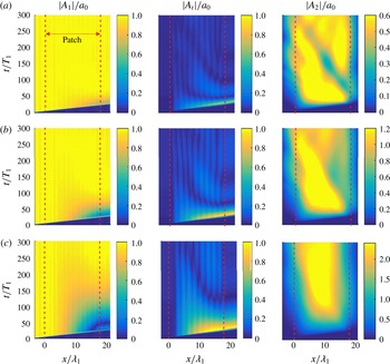
Normalized envelope amplitudes (a)
 $a_{1}^{\ast }$
, (b)
 $a_{t}^{\ast }$
and (c)
 $a_{2}^{\ast }$
, over a bi-chromatic patch, as obtained from (4.3) with
 $\unicode[STIX]{x2202}/\unicode[STIX]{x2202}\bar{t}=0$
. The patch is semi-infinite, starting from
 $x=0$
onward, and the bottom corrugations are given by
 $\unicode[STIX]{x1D701}(x,y)$
for
 $y>0$
and by
 $\unicode[STIX]{x1D701}(x,-y)$
for
 $y<0$
(cf. (4.1)). The amplitude modulations far from the plane of symmetry (i.e. highlighted in the rectangles) are clearly similar to the
 $y$
-invariant solutions (shown in the top figures). We only show the amplitudes for
 $y>0$
since the problem is symmetric with respect to the
 $y=0$
plane. The small vertical arrows show the critical patch width
 $w_{cr_{2}}$
. The physical parameters are
 $\unicode[STIX]{x1D703}_{2}=7\unicode[STIX]{x03C0}/15$
,
 $\unicode[STIX]{x1D703}_{t}=\unicode[STIX]{x1D703}_{2}/2$
,
 $k_{1}h=0.2$
,
 $(d_{1}+d_{2})/h=0.12$
, with (4.8) satisfied. The simulation parameters are
 $\unicode[STIX]{x1D6FF}x/\unicode[STIX]{x1D706}_{1}=0.05$
and
 $\unicode[STIX]{x1D6FF}y/\unicode[STIX]{x1D706}_{1}=0.2$
.

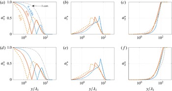
Normalized envelope amplitudes
 $a_{1}^{\ast }$
,
 $a_{t}^{\ast }$
,
 $a_{2}^{\ast }$
at the end of a patch truncated at the critical patch width
 $x=w_{cr_{2}}$
(indicated by a small vertical arrow in figure 5) for
 $\unicode[STIX]{x1D703}_{2}=11\unicode[STIX]{x03C0}/25$
(plots a–c) and
 $\unicode[STIX]{x1D703}_{2}=7\unicode[STIX]{x03C0}/15$
(plots d–f). The
 $x$
-axis is on a logarithmic scale so as to show details near the plane of symmetry. Solid, dashed, and dotted lines represent results obtained for
 $\unicode[STIX]{x1D703}_{t}=0.2\unicode[STIX]{x1D703}_{2}$
,
 $0.5\unicode[STIX]{x1D703}_{2}$
,
 $0.8\unicode[STIX]{x1D703}_{2}$
respectively. The dash-dotted lines show the
 $\boldsymbol{k}_{1}$
-wave and
 $\boldsymbol{k}_{2}$
-wave amplitudes at the end of a monochromatic patch of width
 $w_{cr_{1}}$
. Physical and simulation parameters are the same as those in figure 5.

We show the normalized envelope amplitudes
 $a_{1}^{\ast }$
,
 $a_{t}^{\ast }$
and
 $a_{2}^{\ast }$
obtained for a semi-infinite patch in
 $x$
direction with
 $\unicode[STIX]{x1D703}_{2}=7\unicode[STIX]{x03C0}/15$
and
 $\unicode[STIX]{x1D703}_{t}=\unicode[STIX]{x1D703}_{2}/2$
in figure 5. We have marked in figure 5 the directions of the
 $\boldsymbol{k}_{t}$
and
 $\boldsymbol{k}_{2}$
waves by oblique arrows starting from the origin of each axis. Far from
 $y=0$
, the problem becomes one-dimensional and the separation wavelength between each successive crest and trough of the
 $\boldsymbol{k}_{1}$
or
 $\boldsymbol{k}_{2}$
wave envelope is
 $w_{cr_{2}}=\unicode[STIX]{x03C0}/K_{12}$
as predicted by (4.6) (see the figures on top of each frame that show the
 $y$
-invariant solutions). As for the case of the monochromatic patch, the far field is a function of
 $x$
, i.e. the one-dimensional behaviour is obtained further away from the patch’s plane of symmetry as we look further down in
 $x$
(i.e. considering a longer patch). This comes from the fact that the far-field solution should only be obtained in the region where all three waves co-exist from
 $x=0$
, which is the region given by
 $y>x\cos \unicode[STIX]{x1D703}_{2}$
(i.e. above the vector
 $\boldsymbol{k}_{2}$
in figure 5).
The wave patterns near
 $y=0$
show the remarkable complexity of the three-wave interaction process near the
 $y=0$
plane of symmetry. Generally, wave amplitudes near
 $y=0$
are smaller further down the patch due to the deflection. The qualitative behaviour of waves in each one of the three distinguishable regions (i.e.
 $y/x>\tan \unicode[STIX]{x1D703}_{2}$
,
 $\tan \unicode[STIX]{x1D703}_{2}>y/x>\tan \unicode[STIX]{x1D703}_{t}$
, and
 $y/x<\tan \unicode[STIX]{x1D703}_{t}$
), changes with a change in
 $\unicode[STIX]{x1D703}_{t}$
or
 $\unicode[STIX]{x1D703}_{2}$
. It is to be noted that once we introduce a plane of symmetry at
 $y=0$
, neither
 $a_{1}^{\ast }$
nor
 $a_{t}^{\ast }$
become uniformly zero in
 $y$
at
 $x=w_{cr_{2}}$
(cf. the near field
 $y\sim 0$
and
 $x=w_{cr_{2}}$
in figure 6
a). Therefore, even though the critical patch width minimizes wave energy in the protected wake, there will always be leaked waves emanating near
 $y=0$
at the end of the patch and propagating to the downstream.
Figure 6 shows the variations of the normalized wave amplitudes as functions of
 $y$
at the end of a bi-chromatic patch truncated at
 $x=w_{cr_{2}}$
for
 $\unicode[STIX]{x1D703}_{2}=11\unicode[STIX]{x03C0}/25$
(a–c) and
 $\unicode[STIX]{x1D703}_{2}=7\unicode[STIX]{x03C0}/15$
(d–f). For comparison, we also plot
 $a_{1}^{\ast }$
and
 $a_{2}^{\ast }$
for a monochromatic patch ending at
 $x=w_{cr_{1}}$
(dash-dotted line). Clearly, the bi-chromatic patch achieves a much better reduction in the incident wave amplitude everywhere (cf. figure 6
a,d). The
 $\boldsymbol{k}_{1}$
wave amplitude drops much more quickly in
 $y$
for the bi-chromatic patch, because some of its energy is stored in the hump of
 $\boldsymbol{k}_{t}$
wave energy seen in figure 6(b,e) (note that the horizontal axis is on a logarithmic scale truncated at
 $10^{-1}$
). Using two corrugation modes instead of one thus not only decreases the critical patch width for large
 $\unicode[STIX]{x1D703}_{2}$
, but also spreads out a fraction of the energy leaked near
 $y=0$
further to the sides in the form of
 $\boldsymbol{k}_{t}$
waves. Interestingly, the location of the second hump of
 $\boldsymbol{k}_{1}$
wave energy (figure 6
a,d) scales with
 $1/\sqrt{\cos \unicode[STIX]{x1D703}_{t}}$
, which suggests that the
 $\boldsymbol{k}_{1}\leftrightarrow \boldsymbol{k}_{t}$
wave energy exchange is partially oscillatory in
 $y$
with a period similar to the period of oscillation in the
 $x$
direction (cf.
 $K_{12}$
in (4.9)).
Because the wave amplitudes are shown at the end of the mono- and bi-chromatic patches with width
 $w=w_{cr_{1}}$
and
 $w=w_{cr_{2}}$
, we obtain
 $a_{1}^{\ast }\sim 0$
and
 $a_{2}^{\ast }\sim 1$
for
 $y/\unicode[STIX]{x1D706}_{1}\gg 1$
in figure 6(c,f). In both cases we also observe that the
 $\boldsymbol{k}_{2}$
wave gains energy more rapidly for the smaller
 $\unicode[STIX]{x1D703}_{2}$
angle: for instance, considering the case of
 $\unicode[STIX]{x1D703}_{t}=\unicode[STIX]{x1D703}_{2}/2$
(solid lines), we find that
 $a_{2}^{\ast }=0.9$
at
 $y/\unicode[STIX]{x1D706}_{1}=80\,134$
for
 $\unicode[STIX]{x1D703}_{2}=11\unicode[STIX]{x03C0}/25$
,
 $7\unicode[STIX]{x03C0}/15$
. This suggests that there might be a compromise to be found between deflecting at a very large angle and minimizing the energy content of the transmitted wave beams. The effect of the transitional angle on the amount of energy captured by the
 $\boldsymbol{k}_{2}$
wave is relatively minor, as can be seen from the overlap of the
 $a_{2}^{\ast }$
curves obtained for
 $\unicode[STIX]{x1D703}_{t}=0.2\unicode[STIX]{x1D703}_{2}$
,
 $0.5\unicode[STIX]{x1D703}_{2}$
,
 $0.8\unicode[STIX]{x1D703}_{2}$
in figure 6(c,f).
As a note of caution, we would like to note that the variations of the
 $\boldsymbol{k}_{1}$
wave amplitude are relatively fast close to
 $y=0$
, where
 $a_{1}^{\ast }$
drops from 1 to about 0 in just five wavelengths in figure 5(a) (see also figure 3
a). Similarly,
 $a_{t}^{\ast }$
shows relatively rapid variations in figure 5(b) along the line
 $y=x\cos \unicode[STIX]{x1D703}_{t}$
, as does
 $a_{2}^{\ast }$
in figure 3(b) along the line
 $y=x\cos \unicode[STIX]{x1D703}_{2}$
. The multiple-scale assumption becomes violated when the modulations of the wave envelopes are fast, but here we expect the analytical predictions to remain reasonably valid because the most rapid variations are still five times slower than the carrier wave oscillations. The comparison between theory and direct numerical simulation in the next section will further support this claim as we will demonstrate a very good agreement between the two methods.
5 Direct simulation
A realistic consideration of a patch of seabed bars for coastal protection must take into account all resonance and near-resonance interactions as well as the effect of bottom discontinuities and boundaries. As a general approach to address these, here we use a direct simulation scheme based on a high-order spectral method. The high-order spectral code solves the potential flow equations (2.1) assuming that the solution can be expressed in terms of a convergent series (cf. Zakharov Reference Zakharov1968). It can take up to an arbitrary order of nonlinearity
 $M$
(i.e. number of terms in the perturbation expansion, typically
 $M\sim O(10)$
) and a high number of wave modes
 $N$
(typically
 $N\sim O(10\,000)$
). The method was first formulated by Dommermuth & Yue (Reference Dommermuth and Yue1987) and West et al. (Reference West, Brueckner, Janda, Milder and Milton1987) to model nonlinear wave–wave interactions in deep water. It was then extended to the problems of wave–topography interactions in finite depth (Liu et al.
Reference Liu, Yeh, Lin, Chang and Cho1998; Alam, Liu & Yue Reference Alam, Liu and Yue2010, Reference Alam, Liu and Yue2011), two-layer density stratified fluids (Alam, Liu & Yue Reference Alam, Liu and Yue2009a
,Reference Alam, Liu and Yue
b
), and wave–viscoelastic-seabed interactions (Alam Reference Alam2012b
). The scheme has already undergone extensive convergence tests as well as validations against experimental and other numerical results (e.g. Toffoli et al.
Reference Toffoli, Gramstad, Trulsen, Monbaliu, Bitner-Gregersen and Onorato2010).
In § 5.1 we first demonstrate that the multiple-scale results are in good agreement with direct numerical simulations for an illustrative case study of water-wave deflection by a patch with a plane of symmetry. In § 5.2 we elaborate on the effect of detuning on the performance of the proposed shoreline protection scheme, both numerically and analytically. In § 5.3 we finally investigate the special case of perpendicular deflection, i.e. such that the
 $\boldsymbol{k}_{2}$
waves propagate exactly along the patch.
5.1 Cross-validation
We compare the direct simulation and multiple-scale results of a normal-to-shore monochromatic wavetrain impinging on a bi-chromatic patch with a
 $y=0$
plane of symmetry. The numerical domain is a square of size
 $L_{0}\times L_{0}$
and we select the dimensionless wavenumber
 $k_{1}=110\times (2\unicode[STIX]{x03C0})/L_{0}$
, such that
 $110$
waves of wavelength
 $\unicode[STIX]{x1D706}_{1}$
can fit in the computational space in both
 $x$
and
 $y$
(note in practice that we set
 $L_{0}=2\unicode[STIX]{x03C0}$
for the simplicity of calculations in Fourier space). In the numerical simulations we offset the centreline of the patch (i.e. the
 $y=0$
axis of symmetry) from the centreline of the numerical domain such that we can simulate a patch of width greater than
 $55\unicode[STIX]{x1D706}_{1}$
(the half-width of the numerical domain) in the upper half-plane. Specifically, with this offset we are able to obtain the numerical simulation results in the upper half-plane for a patch of width
 $85\unicode[STIX]{x1D706}_{1}$
; this greatly reduces the computational cost. The solution for the lower half-plane is obtained by symmetry. We use the same parameters as in figures 5 and 6(d–f) such that
 $\unicode[STIX]{x1D703}_{2}=7\unicode[STIX]{x03C0}/15$
,
 $\unicode[STIX]{x1D703}_{t}=\unicode[STIX]{x1D703}_{2}/2$
,
 $k_{1}h=0.2$
and
 $(d_{1}+d_{2})/h=0.12$
with (4.8) satisfied. The seabed bars are laid out from
 $x/\unicode[STIX]{x1D706}_{1}=0$
to
 $x/\unicode[STIX]{x1D706}_{1}=w_{cr_{2}}/\unicode[STIX]{x1D706}_{1}=18.3$
such that the patch width is critical. The incident wave amplitude is taken as
 $a_{0}/h=10^{-3}$
, i.e. two orders of magnitude smaller than the combined seabed bars amplitudes
 $(d_{1}+d_{2})/h=0.12$
, in order to minimize nonlinear wave–wave effects. It is to be noted that we still obtained very similar results for larger wave amplitudes (i.e. such as
 $a_{0}/h=0.02$
), which is expected because the theory is applicable for wave steepness smaller or of same order as the bottom slope.
The generation of the initial waves coming from
 $x<0$
is done using a numerical wavemaker at the beginning of the numerical domain, upstream of the seabed bars. We enforce a radiation condition on the incident and forward-scattered waves at the outgoing boundary, which is several wavelength downstream of the end of the corrugated patch, with the help of a numerical damping layer. The damping layer works efficiently and minimizes spurious reflections because the (right) outgoing boundary is downstream of the corrugated patch (by more than 40 wavelengths
 $\unicode[STIX]{x1D706}_{1}$
), i.e. such that there are no seabed bars there. We also enforce radiation conditions at the side boundaries of the numerical domain (i.e. in
 $y$
) with damping layers. This implies that the patch has a finite width in
 $y$
, since the radiation condition assumes no further energy exchanges between the different wave modes. It should be noted that the damping layers might not work perfectly on the sides of the numerical domain since the water depth is not constant. Spurious reflections are yet minimal as can be seen in the upper half of figure 5. The use of damping layers on the sides of the numerical domain implies that the numerical results are obtained assuming that there are no waves outside of the simulation domain. This is not a problem for waves leaving the domain. However, incident waves unaffected by the seabed bars but propagating in
 $x$
just adjacent to the patch could spread over into the numerical domain by diffraction due to the fact that the neighbouring waves over the patch have non-uniform amplitude. Diffraction effects due to areas of energy dissipation (which can be representative of the situation here where the incident waves cede their energy to other waves) have been addressed by Dalrymple, Kirby & Hwang (Reference Dalrymple, Kirby and Hwang1984), and shown to be relatively minimal such that we do not study them here. Some effects of a patch’s finite transverse length (i.e. here in
 $y$
) have also been reported in the experimental work of Magne, Rey & Ardhuin (Reference Magne, Rey and Ardhuin2005).
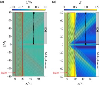
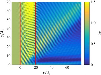
Figure 7(a) shows the normalized wave elevation
 $\unicode[STIX]{x1D702}/a_{0}$
when steady state is reached. The plot is split into two parts, with the lower part (
 $y<0$
) showing the semi-analytical solution (cf. § 4), and with the upper part (
 $y>0$
) showing direct simulation results. As can be seen, analytical and computational results endorse each other, with the same features already described in § 4 standing out: (i) the incident waves propagate unaffected upstream of the patch, (ii) the complex pattern due to the three-wave interactions over the patch becomes
 $y$
-invariant away from the centreline (i.e.
 $|y|\gg \unicode[STIX]{x1D706}_{1}$
), (iii) two beams of
 $\boldsymbol{k}_{1}$
wave energy propagate near
 $y=0$
downstream of the patch (one near the centre at
 $y\sim 0$
and the other at
 $y\sim 15\unicode[STIX]{x1D706}_{1}$
), (iv) a beam of
 $\boldsymbol{k}_{t}$
wave energy emanates from the end of the patch at
 $y\sim \pm 19\unicode[STIX]{x1D706}_{1}$
.
(a) Free-surface elevation
 $\unicode[STIX]{x1D702}/a_{0}$
and (b) time-averaged energy (cf. (5.1)) at the steady state obtained from direct simulation (upper plots
 $y>0$
) and multiple-scale analysis (lower plots
 $y<0$
; cf. (4.3)). A monochromatic wave-train incident from
 $x<0$
impinges on a bi-chromatic patch with parameters
 $\unicode[STIX]{x1D703}_{2}=7\unicode[STIX]{x03C0}/15$
,
 $\unicode[STIX]{x1D703}_{t}=\unicode[STIX]{x1D703}_{2}/2$
,
 $k_{1}=110$
(dimensionless),
 $k_{1}h=0.2$
,
 $(d_{1}+d_{2})/h=0.12$
(with
 $d_{2}/d_{1}$
given by (4.8)),
 $a_{0}/h=10^{-3}$
(cf. figure 2
b). The seabed bars occupy the space between
 $x=0$
and
 $x/\unicode[STIX]{x1D706}_{1}=w_{cr_{2}}/\unicode[STIX]{x1D706}_{1}=18.3$
such that all the incident
 $\boldsymbol{k}_{1}$
wave energy transfers to the target
 $\boldsymbol{k}_{2}$
wave away from the patch’s plane of symmetry
 $y=0$
. The direct simulation parameters are
 $\unicode[STIX]{x1D6FF}x/\unicode[STIX]{x1D706}_{1}=\unicode[STIX]{x1D6FF}y/\unicode[STIX]{x1D706}_{1}=1/9$
and
 $\unicode[STIX]{x1D6FF}t/T_{1}=1/32$
, and the resolution of the multiple-scale solution is the same as in figure 5. The vertical dashed lines show the transects where we plot the maximum free-surface elevation in figure 8.

The protection provided by the bi-chromatic patch can be further highlighted by looking at the time-averaged energy (cf. figure 7 b), i.e.
 $$\begin{eqnarray}\bar{E}(x,y)=\frac{1}{a_{0}^{2}/2}\int _{t_{0}}^{t_{f}}\unicode[STIX]{x1D702}^{2}(x,y,t)\frac{\text{d}t}{t_{f}-t_{0}},\end{eqnarray}$$
where the pre-factor in (5.1) is inversely proportional to the averaged wave energy that would be obtained without the seabed bars. It should be noted that (5.1) is the first-order normalized wave energy, and that it includes contributions from both the kinetic and potential wave energy, which are equal. The time integration is performed when the system reaches steady state with
 $t_{0}/T_{1}=140$
and
 $t_{f}/T_{1}=170$
. A good agreement is obtained for
 $\bar{E}$
in figure 7(b) between the direct simulation (lower half) and the multiple-scale results (upper half). The features described for figure 7(a) also appear in figure 7(b) and are in fact strongly enhanced (e.g.
 $\boldsymbol{k}_{1}$
and
 $\boldsymbol{k}_{t}$
wave beams). The rapid variations of wave energy are due to the formation of a standing-wave pattern downstream of the patch (e.g. along the
 $\boldsymbol{k}_{t}$
wave beam direction) resulting from the superposition of
 $\boldsymbol{k}_{1}$
and
 $\boldsymbol{k}_{t}$
waves. The strongest energy reduction is about 99 % (for both direct simulation and multiple scales) and is achieved within the stripe of width
 $2\unicode[STIX]{x1D706}_{1}$
centred on
 $y=\pm 5\unicode[STIX]{x1D706}_{1}$
.
5.2 Effect of detuning and protection efficiency
To quantify the effect of frequency detuning on the Bragg deflection mechanism, we calculate the maximum free-surface elevation
 $\unicode[STIX]{x1D702}^{\ast }=\max |\unicode[STIX]{x1D702}|/a_{0}$
(in time) with and without detuning along the
 $y$
axis at a virtual shoreline (no reflection considered) that is assumed
 $\unicode[STIX]{x0394}x=26\unicode[STIX]{x1D706}_{1}$
downstream of the patch (i.e. along the dashed lines in figure 7). The incident wave frequency is
 $\unicode[STIX]{x1D714}=\unicode[STIX]{x1D714}_{1}+\unicode[STIX]{x1D71B}$
where
 $\unicode[STIX]{x1D714}_{1}$
is the perfectly tuned wave frequency and
 $\unicode[STIX]{x1D71B}\ll \unicode[STIX]{x1D714}_{1}$
is the detuning parameter. The corresponding detuning wavenumber
 $\unicode[STIX]{x1D705}$
, such that
 $k=k_{1}+\unicode[STIX]{x1D705}$
, is obtained from
 $\unicode[STIX]{x1D71B}=C_{g}\unicode[STIX]{x1D705}$
. In general, detuning effects result in having to solve the time-dependent multiple-scale equations, which can be used also to investigate the transient boundary-value problem of wave group scattering (see e.g. Yu & Mei Reference Yu and Mei2000). For small detuning, however, the frequency detuning
 $\unicode[STIX]{x1D71B}$
can be combined with the slowly varying amplitudes
 $A_{1}$
,
 $A_{t}$
and
 $A_{2}$
in (4.2), i.e., for instance,
 $A_{1}$
is rewritten as
 $A_{1}\exp (-\text{i}\unicode[STIX]{x1D71B}t)$
, such that following the method of Mei (Reference Mei1985) we simply have to replace
 $\unicode[STIX]{x2202}/\unicode[STIX]{x2202}\bar{t}$
by
 $-\text{i}\unicode[STIX]{x1D71B}$
in the envelope equations (4.3). Similarly to the case of class I Bragg reflection, we normalize the detuning frequency by the characteristic long time scale of the system
 $\unicode[STIX]{x1D6FA}_{12}=C_{g}K_{12}$
(cf. (4.7)). The normalized detuning
 $\unicode[STIX]{x1D71B}/\unicode[STIX]{x1D6FA}_{12}$
thus represents the strength of detuning, which suggests that shorter waves are more strongly affected by detuning than longer waves (a detailed analysis of detuning for a bi-chromatic patch infinitely long in
 $y$
direction is provided in appendix B).
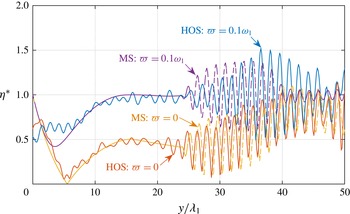
Effect of detuning on the normalized maximum free-surface elevation
 $\unicode[STIX]{x1D702}^{\ast }=\max |\unicode[STIX]{x1D702}|/a_{0}$
at a distance
 $\unicode[STIX]{x0394}x/\unicode[STIX]{x1D706}_{1}=26$
downstream of the patch (i.e. along the dashed lines in figure 7). The detuning parameter is
 $\unicode[STIX]{x1D71B}/\unicode[STIX]{x1D714}_{1}=0$
for the lower two curves and
 $\unicode[STIX]{x1D71B}/\unicode[STIX]{x1D714}_{1}=0.1$
(or
 $\unicode[STIX]{x1D71B}/\unicode[STIX]{x1D6FA}_{12}=3.7$
) for the upper two curves. Other physical parameters are as in figure 7. The direct simulation (HOS) parameters are
 $\unicode[STIX]{x1D6FF}x/\unicode[STIX]{x1D706}_{1}=\unicode[STIX]{x1D6FF}y/\unicode[STIX]{x1D706}_{1}=1/7.3$
and
 $\unicode[STIX]{x1D6FF}t/T_{1}=1/32$
, and the resolution of the multiple-scale solution (MS) is the same as in figure 5. Detuning clearly results in a larger maximum wave amplitude downstream of the patch.

The result of our numerical experiments on the effect of detuning is presented in figure 8. In the absence of detuning, i.e.
 $\unicode[STIX]{x1D71B}=0$
, a global minimum of
 $\unicode[STIX]{x1D702}^{\ast }$
for both direct simulation and multiple scales is observed: this minimum in
 $\unicode[STIX]{x1D702}^{\ast }$
corresponds to the minimum of incident wave amplitude
 $a_{1}^{\ast }$
at the end of the patch as seen in figure 6(d) (dotted line at
 $y/\unicode[STIX]{x1D706}_{1}\sim 6$
). The large standing-wave oscillations seen for
 $y/\unicode[STIX]{x1D706}_{1}>25$
are, as mentioned previously, due to the superposition of the leaked
 $\boldsymbol{k}_{1}$
and
 $\boldsymbol{k}_{t}$
waves and predicted by both methods. Of course, the superposition would not occur if we were to observe
 $\unicode[STIX]{x1D702}^{\ast }$
further downstream of the patch since the
 $\boldsymbol{k}_{t}$
beams of energy propagate progressively away from the
 $y=0$
plane of symmetry to which the
 $\boldsymbol{k}_{1}$
beams of energy are confined.
The effect of detuning on the maximum free-surface elevation is strongest away from the
 $y=0$
plane of symmetry. There is still a global minimum near
 $y=0$
for
 $\unicode[STIX]{x1D71B}/\unicode[STIX]{x1D6FA}_{12}=3.7$
but
 $\unicode[STIX]{x1D702}^{\ast }$
reaches a unitary value (which corresponds to no wave amplitude reduction) near
 $y=15\unicode[STIX]{x1D706}_{1}$
, with oscillations farther out to the sides again due to the superposition of
 $\boldsymbol{k}_{1}$
and
 $\boldsymbol{k}_{t}$
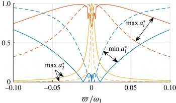
waves. The wave field away from
 $y=0$
changes radically because the second interaction of the two-step Bragg resonance mechanism, which is key to reducing the incident wave mode energy far from the plane of symmetry, is more strongly impacted than the first Bragg interaction. The fact that detuning affects the successive Bragg interactions cumulatively is further discussed in appendix B for the case of an infinitely long patch (see figures 12 and 13).
Quantitative differences between direct simulation and multiple-scale results are in general expected and obtained here (as is seen in figure 8). The discrepancies are due to the fact that first-order multiple scales neglects wave–wave nonlinearities, higher-order wave–bottom interactions and the effect of discontinuity in the seabed topography at the beginning and end of the patch. This latter item is known to result in, among other effects, evanescent modes near boundaries. In the absence of detuning (cf. lower two curves in figure 8), the maximum free-surface elevation obtained from the direct simulation matches well with the multiple-scale solution except for a small local peak near
 $y=0$
and for the small oscillations from
 $y=0$
to
 $y=25\unicode[STIX]{x1D706}_{1}$
. The discrepancy at
 $y=0$
can be expected, even though the bottom variations are continuous there, because as discussed before the variations of the wave amplitudes near the patch’s plane of symmetry predicted by the theory are relatively rapid (
 $\unicode[STIX]{x1D702}^{\ast }$
drops to 0 in approximately 5 wavelengths, cf. figure 8, and discussion at the end of § 4): weak diffraction effects may be obtained here that are considered in the numerical solution but not in the theoretical solution. These relatively fast variations, which are not as rapid in direct simulation, potentially contribute to the small phase shift observed between theory and experiment for the location of the superposed
 $\boldsymbol{k}_{1}$
and
 $\boldsymbol{k}_{t}$
waves. Similar discrepancies between the two methods are observed for the detuned case (upper two curves in figure 8), and are higher (in particular far from the patch’s plane of symmetry), which is consistent with the fact that multiple-scale performs best at perfect resonance, i.e. in the absence of detuning. Despite the simplifying assumptions of multiple-scale analysis, the comparison in figure 8 is however still good almost everywhere in the domain, with or without detuning.
(a) Protection efficiency
 ${\mathcal{P}}$
(5.2) with and without detuning (
 $\unicode[STIX]{x1D71B}/\unicode[STIX]{x1D714}_{1}=0$
, 0.01, 0.03, 0.05, 0.1 which corresponds to
 $\unicode[STIX]{x1D71B}/\unicode[STIX]{x1D6FA}_{12}=0$
, 0.37, 1.1, 1.8, 3.7) at a distance
 $\unicode[STIX]{x0394}x=26\unicode[STIX]{x1D706}_{1}$
downstream of the patch (i.e. at
 $x=w_{cr_{2}}+26\unicode[STIX]{x1D706}_{1}$
, which is along the dashed line in figure 7). The results are obtained from multiple-scale analysis. (b) Close-up with direct simulation results added for
 $\unicode[STIX]{x1D71B}/\unicode[STIX]{x1D714}_{1}=0,0.1$
(dashed lines). The physical and simulation parameters other than
 $\unicode[STIX]{x1D71B}$
are the same as those in figure 8.

To further assess the efficiency of the Bragg deflection mechanism, as well as how it is affected by detuning, we now define a protection efficiency variable
 ${\mathcal{P}}$
, where
 $$\begin{eqnarray}{\mathcal{P}}(x,y)=1-\frac{1}{y}\int _{0}^{y}\bar{E}(x,\unicode[STIX]{x1D70F})\,\text{d}\unicode[STIX]{x1D70F}.\end{eqnarray}$$
The protection efficiency
 ${\mathcal{P}}$
measures the
 $y$
-average wave energy reduction (with
 $\bar{E}$
obtained at steady state and given in (5.1)) on a line parallel and downstream of the patch’s trailing edge. Figure 9(a) shows
 ${\mathcal{P}}$
over a relatively large domain, i.e. from
 $y=0$
to
 $y=350\unicode[STIX]{x1D706}_{1}$
, with
 $\bar{E}$
evaluated at the distance
 $\unicode[STIX]{x0394}x=26\unicode[STIX]{x1D706}_{1}$
downstream of the patch. Figure 9(b) is a close-up with the addition of direct simulation results (dashed lines), to show that the multiple-scale predictions are reasonably accurate, even with 10 % detuning.
Time-averaged energy
 $\bar{E}$
(cf. (5.1),
 $t_{0}/T_{1}=140$
,
 $t_{f}/T_{1}=170$
) obtained from direct simulation for a patch with a plane of symmetry at
 $y=0$
. The physical and simulation parameters are identical to those in figure 7 except for the deflection angle which is now set to
 $\unicode[STIX]{x1D703}_{2}=\unicode[STIX]{x03C0}/2$
. The energy distribution is symmetric with respect to the
 $y=0$
axis which is why we only show the upper half-plane
 $y>0$
. The solid vertical lines show the beginning and end of the corrugated patch in
 $x$
direction.

The protection efficiency
 ${\mathcal{P}}$
for perfectly tuned waves (i.e.
 $\unicode[STIX]{x1D71B}=0$
) is as high as 88 % at
 $y=270\unicode[STIX]{x1D706}_{1}$
, meaning that only 12 % of the incident wave energy makes it inside the protected wake behind the patch. From
 $y\sim 270\unicode[STIX]{x1D706}_{1}$
farther out to the sides,
 ${\mathcal{P}}$
starts decreasing because the deflected
 $\boldsymbol{k}_{2}$
waves, which captured most of the incident wave energy, propagate within the semi-infinite space
 $y>x/\cos \unicode[STIX]{x1D703}_{2}$
outside of the protected wake, which includes the half-line
 $y>270\unicode[STIX]{x1D706}_{1}>26\unicode[STIX]{x1D706}_{1}/\cos (7\unicode[STIX]{x03C0}/15)$
. As already discussed, the protection efficiency decreases rapidly with an increase in
 $\unicode[STIX]{x1D71B}$
away from
 $y=0$
since the two-step Bragg deflection mechanism is relatively sensitive to detuning. Detuning affects transmitted waves (as in Bragg deflection) more strongly than reflected waves, because transmitted waves have an oscillatory behaviour over the corrugations: detuning not only diminishes wave–bottom interactions but also changes the critical patch width where the incident wave amplitude reaches a minimum. Nonetheless, we can see that significant wave amplitude reduction is still achieved over a large domain with some small detuning.
5.3 Perpendicular deflection
In this section we investigate with direct numerical simulation the special case of shore-normal incident waves (with wavenumber
 $\boldsymbol{k}_{1}=k_{1}\hat{x}$
) that are deflected by
 $90^{\circ }$
(i.e. perpendicularly) into shore-parallel resonated waves (
 $\boldsymbol{k}_{2}=\pm k_{2}{\hat{y}}$
, cf. figure 2
b). Assuming perfectly tuned incident waves, we first show in figure 10 that the averaged wave energy (5.1) is again significantly decreased in the wake of the patch for
 $y<x\cos \unicode[STIX]{x1D703}_{t}$
. A bi-chromatic patch can therefore deflect incident waves to the shore-parallel direction, and offer shore protection near the patch’s plane of symmetry. It is to be noted that the physical parameters in figure 10 are the same as those in figure 7 (except for
 $\unicode[STIX]{x1D703}_{2}=\unicode[STIX]{x03C0}/2$
in figure 10), such that the patch width in figure 10 is not critical. Wave reduction is thus obtained in the wake near the patch’s plane of symmetry regardless of its width.
Far from the plane of symmetry where the solution is expected to be
 $y$
-invariant, the synchronization condition (4.8) suggests that the bi-chromatic patch should be turned into a monochromatic patch since we get
 $d_{2}/d_{1}\rightarrow 0$
when
 $\unicode[STIX]{x1D703}_{2}\rightarrow 0$
. However, as was mentioned earlier, the degeneracy of the Bragg resonance condition prevents a monochromatic patch from deflecting incident waves by a
 $\unicode[STIX]{x1D703}_{2}=\unicode[STIX]{x03C0}/2$
angle. Therefore the solution (4.4) is not valid for perpendicular deflection and we should still consider a bi-chromatic patch (with
 $d_{1}$
,
 $d_{2}\neq 0$
). Let us now suppose that the envelope amplitude
 $A_{2}$
need not be continuous at the patch boundaries, i.e. at
 $x=0$
or
 $x=w$
. Then, the steady-state (
 $\unicode[STIX]{x2202}/\unicode[STIX]{x2202}\bar{t}\equiv 0$
)
 $y$
-invariant solution (
 $\unicode[STIX]{x2202}/\unicode[STIX]{x2202}\bar{y}\equiv 0$
) of (4.3) with
 $\unicode[STIX]{x1D703}_{2}=\unicode[STIX]{x03C0}/2$
is obtained as
 $$\begin{eqnarray}A_{1}=a_{0},\quad A_{t}=0,\quad A_{2}=\frac{d_{1}\cos \unicode[STIX]{x1D703}_{t}}{d_{2}\cos (\unicode[STIX]{x1D703}_{2}-\unicode[STIX]{x1D703}_{t})}a_{0}.\end{eqnarray}$$
The incident wave amplitude in (5.3) is found to remain unchanged over the patch, which is in agreement with the conservation of wave action (4.5). If (5.3) is correct, then, a bi-chromatic patch set to deflect waves by a
 $90^{\circ }$
angle cannot be expected to protect the shore far from the patch’s plane of symmetry. This result is now validated in figure 11 as we show the evolution in time of the envelope amplitudes over a patch infinitely long in
 $y$
direction (and therefore the solution is independent of
 $y$
) and for which
 $\unicode[STIX]{x1D703}_{2}=\unicode[STIX]{x03C0}/2$
. We provide three different cases of ripple amplitudes, i.e.
 $d_{1}/d_{2}=0.5,1,2$
(see figure 11
a–c), in order to verify the linear relationship predicted in (5.3) between the amplitude of the deflected waves
 $|A_{2}|$
and the ratio
 $d_{1}/d_{2}$
. The incident and resonated envelope amplitudes are obtained from direct simulation and are extracted from the overall free-surface solution by fast Fourier transform in
 $y$
direction. We then also average in time over the carrier wave period (i.e.
 $T_{1}$
) in order to remove the fast oscillations of the carrier wave phases. It should be noted that the wave amplitude is zero for all three modes for
 $t<k_{1}(x-x_{w})/\unicode[STIX]{x1D714}$
in figure 11 since the incident waves start propagating into the domain through the wavemaker on the left-hand side (at
 $x=x_{w}$
) only at
 $t=0$
.
Evolution of the envelope amplitudes
 $|A_{1}|/a_{0}$
,
 $|A_{t}|/a_{0}$
and
 $|A_{2}|/a_{0}$
in
 $x$
and
 $t$
for waves incident from
 $x<0$
and propagating over an infinitely long patch in
 $y$
direction with
 $\unicode[STIX]{x1D703}_{2}=2\unicode[STIX]{x1D703}_{t}=\unicode[STIX]{x03C0}/2$
. We consider three different distributions of ripple amplitudes: (a)
 $d_{1}/d_{2}=0.5$
, (b)
 $d_{1}/d_{2}=1$
, (c)
 $d_{1}/d_{2}=2$
and keep
 $(d_{1}+d_{2})/h=0.12$
fixed. The results in the right column demonstrate that
 $|A_{2}|$
increases approximately linearly with
 $d_{1}/d_{2}$
. The patch width is
 $w/\unicode[STIX]{x1D706}_{1}=17.5$
and the other physical parameters are
 $k_{1}h=0.2$
,
 $a_{0}/h=10^{-3}$
. The direct simulation parameters are
 $\unicode[STIX]{x1D6FF}x/\unicode[STIX]{x1D706}_{1}=\unicode[STIX]{x1D6FF}y/\unicode[STIX]{x1D706}_{1}=1/7.31$
and
 $\unicode[STIX]{x1D6FF}t/T_{1}=1/32$
.

In all cases, we see that the
 $\boldsymbol{k}_{1}\leftrightarrow \boldsymbol{k}_{t}$
Bragg interaction is strongest at the initial time:
 $|A_{t}|$
increases very rapidly to the detriment of
 $|A_{1}|$
(figure 11
a,b in the left and middle columns). The duration and significance of energy transfer from the
 $\boldsymbol{k}_{1}$
to the
 $\boldsymbol{k}_{t}$
waves increases with increasing
 $d_{1}/d_{2}$
(i.e. from figure 11
a to 11
c), which is expected because the strength of the
 $\boldsymbol{k}_{1}\leftrightarrow \boldsymbol{k}_{t}$
Bragg interaction is proportional to
 $d_{1}\cos \unicode[STIX]{x1D703}_{t}$
. Energy exchanges still occur at later times, as seen from the small oscillations of
 $|A_{t}|$
, but the incident wave energy eventually becomes fully transmitted such that
 $|A_{1}|$
is as large downstream and upstream of the patch (i.e.
 $|A_{1}|/a_{0}\sim 1$
at the end of the patch). The
 $\boldsymbol{k}_{2}$
wave amplitude
 $|A_{2}|$
also only increases early on, with some energy redistribution clearly seen across the patch at later times for the smaller
 $d_{1}/d_{2}$
(figure 11
a–c in the right column). In particular, we find that the plateau reached by the
 $x$
-averaged
 $|A_{2}|$
amplitude grows approximately linearly with
 $d_{1}/d_{2}$
, which means that (5.3) is a good first-order approximation to the
 $y$
-invariant problem. That the initial net energy flow from
 $|A_{1}|$
to
 $|A_{2}|$
increases linearly with
 $d_{1}/d_{2}$
(note that the colour map scales change between figures) is somewhat surprising since larger
 $d_{1}$
imply smaller
 $d_{2}$
, hence weaker
 $\boldsymbol{k}_{t}\leftrightarrow \boldsymbol{k}_{2}$
Bragg interactions. However, since
 $\boldsymbol{k}_{2}$
waves are trapped by the patch for
 $\unicode[STIX]{x1D703}_{2}=\unicode[STIX]{x03C0}/2$
, they experience an infinite number of Bragg interactions for an infinitely long patch in
 $y$
direction. The second Bragg interaction is therefore intrinsically much more efficient than the first
 $\boldsymbol{k}_{1}\leftrightarrow \boldsymbol{k}_{t}$
Bragg interaction, which becomes the limiting mechanism in the overall transfer of
 $\boldsymbol{k}_{1}$
wave energy to the
 $\boldsymbol{k}_{2}$
waves.
To summarize our results on perpendicular deflection, we found that the case of
 $\unicode[STIX]{x1D703}_{2}=\unicode[STIX]{x03C0}/2$
offers significant wave energy reduction in the downstream near the patch’s plane of symmetry. However, no protection can be obtained when
 $\unicode[STIX]{x1D703}_{2}=\unicode[STIX]{x03C0}/2$
far from the patch’s plane of symmetry, because the conservation of wave action requires waves in the downstream propagating with a non-zero velocity in
 $x$
direction. How much far away from
 $y=0$
we get the
 $y$
-invariant behaviour is therefore of significance importance and can be estimated, to a good first-order approximation, by inspection of the steady-state solution (5.3). Indeed, the far field is expected to start where the deflected wave amplitude
 $|A_{2}|$
obtained for a patch with a plane of symmetry becomes as large as the
 $y$
-invariant solution (5.3), i.e. at a distance
 $|y|>0$
such that
 $|A_{2}(y)|/a_{0}=(d_{1}\cos \unicode[STIX]{x1D703}_{t})/[d_{2}\cos (\unicode[STIX]{x1D703}_{2}-\unicode[STIX]{x1D703}_{t})]$
. For the results of figure 10, we find that
 $|A_{2}|$
increases approximately linearly with
 $|y|$
. We estimated the growth slope to be
 ${\sim}0.02$
per wavelength
 $\unicode[STIX]{x1D706}_{1}$
, such that the maximum value predicted by (5.3), i.e.
 $|A_{2}|/a_{0}=3.4$
, is reached at
 $y/\unicode[STIX]{x1D706}_{1}=160$
in this case.
6 Concluding remarks
We investigated the deflection of water waves incident on a patch of oblique seabed bars via multiple-scale analysis and direct numerical simulation. Unlike the Bragg reflection mechanism in which waves may get trapped and hence amplified in the area between the coastline and a patch of seabed bars, the Bragg deflection mechanism can be reliable for protecting natural coastlines because all waves are transmitted such that any form of trapping is completely ruled out. The proposed patch of seabed corrugations for shore protection has a plane of symmetry at
 $y=0$
(the
 $y$
axis is parallel to the incident wave crests, see figure 2), such that incident waves propagating in the upper half-plane
 $y>0$
(resp.
 $y<0$
) are deflected toward
 $y=+\infty$
(resp.
 $y=-\infty$
). At resonance frequency, the deflection of the incident waves to the sides of the patch’s plane of symmetry results in a wake of decreased wave activity, i.e. where the water is calm. The extent of the protected wake in the
 $y$
direction grows further to the downstream (in
 $x$
), and can be theoretically infinite provided that the patch is likewise infinite in the
 $y$
direction. For the case study of § 5, the corrugated patch provides an average 88 % energy reduction against perfectly tuned waves in the protected wake, with the 12 % remaining wave energy in the downstream being leaked in the form of beams of energy emanating near the patch’s plane of symmetry.
We showed that achieving a large protected wake (which requires the deflection of incident waves at a large angle), requires the use of a bi-chromatic patch instead of a monochromatic patch. The deflection of waves at or close to a
 $90^{\circ }$
angle is impossible using mono-modal corrugations because the Bragg resonance condition is degenerate in this case. With bi-modal corrugations, however, we demonstrated that the deflection at a large angle is achievable provided that a transitional wave mediates the energy transfer from the incident wave mode to the target deflected wave. The corresponding resonance mechanism was referred to as a class I
 $_{2}$
Bragg resonance since it is a first-order two-step Bragg interaction which requires bi-modal corrugations.
We demonstrated that the (critical) patch width which provides the best protection can be obtained analytically assuming that the patch is infinitely long in the
 $y$
direction, and that it is equal to approximately 20 incident wave wavelengths when the total ripple amplitude is 0.12 times the water depth (cf. figure 4
c). With a wave period of 10 s and a water depth of 5 m (such that the incident wavelength is about 67 m), the corrugated patch investigated in § 5 (see e.g. caption of figure 7) covers a zone 1.3 km long, that includes four (
 $\boldsymbol{k}_{b_{1}}$
) bar crests and twelve (
 $\boldsymbol{k}_{b_{2}}$
) bar crests in the
 $x$
direction.
We showed that the protection efficiency of the class I
 $_{2}$
Bragg deflection mechanism is relatively robust to small frequency detuning, i.e. such that significant protection (
 ${>}50\,\%$
) is obtained for
 ${\sim}2\,\%$
detuning. The protection efficiency however diminishes significantly with further detuned waves (i.e. with 10 % detuning), in which case a good protection against a broadband incident wave spectrum can still be obtained using a superposition of corrugated patches (cf. e.g. Alam Reference Alam2012a
).
We have assumed that the incident waves were normal to the corrugated patch, i.e. parallel to the shoreline, because the angle of incident waves near shore should remain small in general due to wave refraction (cf. e.g. Herbers, Elgar & Guza Reference Herbers, Elgar and Guza1999). In the near shore, the presence of sloping beaches indeed results in refraction effects which tend to make the wave crests parallel to the shore. In the case where the incidence angle is not exactly zero but small, a resonance can still be obtained, but which requires careful analysis. The key idea is to represent the effect of oblique incidence as a slow modulation of the incident waves, whose primary wavenumber and frequency are kept as the perfectly tuned Bragg wavenumber and frequency. Therefore, the effect of oblique incidence is similar to that of frequency detuning (cf. e.g. Kirby Reference Kirby1993). For small incidence angle we thus rewrite the incident wave phase
 $\boldsymbol{k}\boldsymbol{\cdot }\boldsymbol{x}-\unicode[STIX]{x1D714}t$
as
 $$\begin{eqnarray}\boldsymbol{k}\boldsymbol{\cdot }\boldsymbol{x}-\unicode[STIX]{x1D714}t=k_{1}x-\unicode[STIX]{x1D714}_{1}t+(\unicode[STIX]{x1D705}_{x}x+\unicode[STIX]{x1D705}_{y}y-\unicode[STIX]{x1D71B}t),\end{eqnarray}$$
where
 $k_{1}$
and
 $\unicode[STIX]{x1D714}_{1}$
are the Bragg resonant wavenumber and frequency and
 $\unicode[STIX]{x1D705}_{x}$
,
 $\unicode[STIX]{x1D705}_{y}$
(
 $\ll k_{1}$
) and
 $\unicode[STIX]{x1D71B}$
(
 $\ll \unicode[STIX]{x1D714}_{1}$
) the detuning wavenumbers and frequency. Similarly to the case of frequency detuning, the envelope amplitudes
 $A_{1}$
,
 $A_{t}$
, and
 $A_{2}$
are rewritten as
 $A_{1}\exp (-\text{i}\unicode[STIX]{x1D71B}t)$
,
 $A_{t}\exp (-\text{i}\unicode[STIX]{x1D71B}t)$
, and
 $A_{2}\exp (-\text{i}\unicode[STIX]{x1D71B}t)$
, with the new variables
 $A_{1}$
,
 $A_{t}$
, and
 $A_{2}$
solutions of (4.2) with
 $\unicode[STIX]{x2202}/\unicode[STIX]{x2202}\bar{t}$
substituted with
 $-\text{i}\unicode[STIX]{x1D71B}$
. Because here we only consider the case of small incidence angle, the group velocity of the incident waves remains
 $\boldsymbol{C}_{g_{1}}=C_{g}\hat{x}$
, i.e. the waves propagate along the
 $x$
axis, such that the problem requires no boundary conditions for
 $A_{1}$
in
 $y$
. The boundary conditions then are
 $A_{1}=a_{0}\exp (-\text{i}\unicode[STIX]{x1D705}_{y}y)$
and
 $A_{t}=A_{2}=0$
at
 $x=0$
, and
 $A_{t}=A_{2}=0$
at
 $y=0$
, for both the upper and the lower patch. Importantly, the solution over the upper patch is not the mirror of the solution over the lower patch anymore, i.e.
 $A_{1}(x,-y)$
for
 $y<0$
is not the same as
 $A_{1}(x,y)$
for
 $y>0$
, since the boundary condition for
 $A_{1}$
at
 $x=0$
(i.e. along the
 $y$
axis) is not an even function of
 $y$
. This is consistent with the fact that the oblique incidence breaks the symmetry of the problem. When the incidence angle becomes close to 0, we have
 $\unicode[STIX]{x1D705}_{x},\unicode[STIX]{x1D705}_{y}\rightarrow 0$
such that
 $\unicode[STIX]{x1D71B}\rightarrow 0$
, and the boundary condition for the incident wave at the beginning of the patch, i.e.
 $A_{1}(x=0)=a_{0}\exp (-\text{i}\unicode[STIX]{x1D705}_{y}y)$
, becomes uniform in
 $y$
. This indicates that the solution for oblique incidence tends asymptotically to the solution for normal incidence as
 $\unicode[STIX]{x1D705}_{x},\unicode[STIX]{x1D705}_{y}\rightarrow 0$
.
In the case of perpendicular deflection, when the incident and final resonated waves are perpendicular, we found that the incident wave energy stops flowing to the deflected waves far from the patch’s plane of symmetry after relatively short transients. As a result, the protection offered by a patch set to deflect waves at a
 $90^{\circ }$
angle is of limited extent in the
 $y$
direction, and restricted to the neighbourhood of the patch’s plane of symmetry. Perpendicular deflection also results in leaked waves, which, once reflected by a shoreline, can excite waves propagating along the patch in a way that water-wave trapping becomes again possible. This is, of course, an undesirable feature as explained by Yu & Mei (Reference Yu and Mei2000) for the case of shore-parallel seabed bars. The formation of waves that propagate parallel to the patch may be, however, relevant to the analysis of topographically trapped waves, also known as Bloch waves, as the excitation of such waves by free modes remains of contemporary interests (cf. Porter & Porter Reference Porter and Porter2001).
The application of the class I
 $_{2}$
Bragg deflection of water waves for shore protection has been shown to be reliable in the sense that the achievement of a calm buffer zone downstream of the patch is robust against reflections from a reflecting shoreline either straight or curved. Several improvements can be done regarding the theory, in particular with respect to the effect of viscosity (which is expected to be small, see e.g. Couston et al.
Reference Couston, Guo, Chamanzar and Alam2015), higher-order wave–bottom terms and finite-amplitude waves. Practical issues related to the realization of man-made small breakwaters or to their stability in sandy/muddy areas are also important challenges (Bailard et al.
Reference Bailard, DeVries, Kirby and Guza1991; Burcharth et al.
Reference Burcharth, Kramer, Lamberti and Zanuttigh2006), and while beyond the scope of the current manuscript, they must be considered thoroughly. For instance, scouring around submerged seabed bars may affect the effectiveness of the protection scheme, as well as put the man-made structure at risk of sinking (Kramer et al.
Reference Kramer, Zanuttigh, Van der Meer, Vidal and Gironella2005; Khan-Mozahedy et al.
Reference Khan-Mozahedy, Muñoz Perez, Neves, Sancho and Cavique2016). The effect of seabed bars on local sediment transports is also of general interest for the dynamics of coastal processes, in particular because seabed bars can decrease beach erosion (Bailard et al.
Reference Bailard, DeVries and Kirby1992). The details of shoreline response to submerged structures are however complex and far from fully resolved (Ranasinghe & Turner Reference Ranasinghe and Turner2006). We finally note that laboratory experiments of Bragg resonance have already been successfully conducted in both two-dimensional (e.g. Weidman et al.
Reference Weidman, Herczynski, Yu and Howard2015) and three-dimensional settings (Elandt, Shakeri & Alam Reference Elandt, Shakeri and Alam2014), such that an experimental demonstration of class I
 $_{2}$
Bragg resonance should be possible with existing technology.
Appendix A
The evolution of the incident and resonated wave amplitudes (
 $A_{1}$
,
 $A_{t}$
and
 $A_{2}$
) over a bi-chromatic patch with corrugations
 $\unicode[STIX]{x1D701}$
given by (4.1) can be found using multiple scales by considering a first-order potential
 $\unicode[STIX]{x1D719}^{(1)}$
of the form
 $$\begin{eqnarray}\unicode[STIX]{x1D719}^{(1)}=\unicode[STIX]{x1D6FC}_{1}(z)\text{e}^{\text{i}(\boldsymbol{k}_{1}\boldsymbol{\cdot }\boldsymbol{x}-\unicode[STIX]{x1D714}t)}+\unicode[STIX]{x1D6FC}_{t}(z)\text{e}^{\text{i}(\boldsymbol{k}_{t}\boldsymbol{\cdot }\boldsymbol{x}-\unicode[STIX]{x1D714}t)}+\unicode[STIX]{x1D6FC}_{2}(z)\text{e}^{\text{i}(\boldsymbol{k}_{2}\boldsymbol{\cdot }\boldsymbol{x}-\unicode[STIX]{x1D714}t)}+\text{c.c.},\end{eqnarray}$$
where
 $$\begin{eqnarray}\unicode[STIX]{x1D6FC}_{j}(z;\bar{x},\bar{y},\bar{t})=\frac{A_{j}(\bar{x},\bar{y},\bar{t})}{2}\frac{g}{\unicode[STIX]{x1D714}}\frac{\cosh [k_{1}(z+h)]}{\cosh (k_{1}h)},\quad j=1,t,2.\end{eqnarray}$$
The governing equation for
 $A_{1}$
,
 $A_{t}$
and
 $A_{2}$
can then be obtained from the solvability condition, which ensures that a bounded second-order potential of the form
 $$\begin{eqnarray}\unicode[STIX]{x1D719}^{(2)}=\unicode[STIX]{x1D713}_{1}(z)\text{e}^{\text{i}(\boldsymbol{k}_{1}\boldsymbol{\cdot }\boldsymbol{x}-\unicode[STIX]{x1D714}t)}+\unicode[STIX]{x1D713}_{t}(z)\text{e}^{\text{i}(\boldsymbol{k}_{t}\boldsymbol{\cdot }\boldsymbol{x}-\unicode[STIX]{x1D714}t)}+\unicode[STIX]{x1D713}_{2}(z)\text{e}^{\text{i}(\boldsymbol{k}_{2}\boldsymbol{\cdot }\boldsymbol{x}-\unicode[STIX]{x1D714}t)}+\mathit{locked~waves}+\text{c.c.},\end{eqnarray}$$
satisfies the second-order problem. In (A 3), the slow variations of the amplitudes
 $\unicode[STIX]{x1D713}_{1}$
,
 $\unicode[STIX]{x1D713}_{t}$
and
 $\unicode[STIX]{x1D713}_{2}$
only affect the third-order solution and, as a result, they can be neglected in the present derivation. The expression locked waves designates non-resonant terms of the second-order solution which do not play any role in obtaining the evolutionary equations for
 $A_{1}$
,
 $A_{t}$
and
 $A_{2}$
. At the second order in bottom steepness
 $O(\unicode[STIX]{x1D716}^{2})$
, the governing equations obtained neglecting wave–wave interactions read
 $$\begin{eqnarray}\displaystyle & \displaystyle \unicode[STIX]{x1D6FB}^{2}\unicode[STIX]{x1D719}^{(2)}+(\unicode[STIX]{x1D735}_{h}\boldsymbol{\cdot }\bar{\unicode[STIX]{x1D735}}+\bar{\unicode[STIX]{x1D735}}\boldsymbol{\cdot }\unicode[STIX]{x1D735}_{h})\unicode[STIX]{x1D719}^{(1)}=0,\quad \text{in }-h\leqslant z\leqslant 0, & \displaystyle\end{eqnarray}$$
 $$\begin{eqnarray}\displaystyle & \displaystyle \unicode[STIX]{x1D719}_{tt}^{(2)}+g\unicode[STIX]{x1D719}_{z}^{(2)}+2\unicode[STIX]{x1D719}_{t\bar{t}}^{(1)}=0,\quad \text{on }z=0, & \displaystyle\end{eqnarray}$$
 $$\begin{eqnarray}\displaystyle & \displaystyle \unicode[STIX]{x1D716}\unicode[STIX]{x1D719}_{z}^{(2)}=-\unicode[STIX]{x1D716}\bar{\unicode[STIX]{x1D735}}h\boldsymbol{\cdot }\unicode[STIX]{x1D735}_{h}\unicode[STIX]{x1D719}^{(1)}+\unicode[STIX]{x1D735}_{h}\boldsymbol{\cdot }(\unicode[STIX]{x1D701}\unicode[STIX]{x1D735}_{h}\unicode[STIX]{x1D719}^{(1)}),\quad \text{on }z=-h, & \displaystyle\end{eqnarray}$$
 $\bar{\unicode[STIX]{x1D735}}=(\unicode[STIX]{x2202}_{\bar{x}},\unicode[STIX]{x2202}_{\bar{y}})$
. In (A 4a
), we note that
 $\bar{\unicode[STIX]{x1D735}}$
and
 $\unicode[STIX]{x1D735}_{h}$
do not commute because of the simultaneous fast and slow spatial variations of the wave phases. Substituting (A 1) and (A 3) in (A 4) we have for each wave mode, i.e. for
 $j=1,t,2$
,
 $$\begin{eqnarray}\displaystyle & \displaystyle \unicode[STIX]{x1D713}_{j,zz}-k_{1}^{2}\unicode[STIX]{x1D713}_{j}=-\text{i}\left[\bar{\unicode[STIX]{x1D735}}\boldsymbol{\cdot }(\boldsymbol{k}_{j}\unicode[STIX]{x1D6FC}_{j})+\boldsymbol{k}_{j}\boldsymbol{\cdot }\bar{\unicode[STIX]{x1D735}}\unicode[STIX]{x1D6FC}_{j}\right],\quad \text{in }-h\leqslant z\leqslant 0, & \displaystyle\end{eqnarray}$$
 $$\begin{eqnarray}\displaystyle & \displaystyle -\unicode[STIX]{x1D714}^{2}\unicode[STIX]{x1D713}_{j}+g\unicode[STIX]{x1D713}_{j,z}=2\text{i}\unicode[STIX]{x1D714}\unicode[STIX]{x1D6FC}_{j,\bar{t}},\quad \text{on }z=0, & \displaystyle\end{eqnarray}$$
 $$\begin{eqnarray}\displaystyle & \displaystyle \unicode[STIX]{x1D716}\unicode[STIX]{x1D713}_{j,z}=\unicode[STIX]{x1D6FE}_{jm}\unicode[STIX]{x1D6FC}_{m}-\text{i}\unicode[STIX]{x1D716}(\bar{\unicode[STIX]{x1D735}}h)\boldsymbol{\cdot }(\boldsymbol{k}_{j}\unicode[STIX]{x1D6FC}_{j}),\quad \text{on }z=-h, & \displaystyle\end{eqnarray}$$
 $\unicode[STIX]{x1D6FE}_{11}=\unicode[STIX]{x1D6FE}_{12}=\unicode[STIX]{x1D6FE}_{tt}=\unicode[STIX]{x1D6FE}_{21}=\unicode[STIX]{x1D6FE}_{22}=0$
, and
 $\unicode[STIX]{x1D6FE}_{1t}=\unicode[STIX]{x1D6FE}_{t1}=-(d_{1}/2)\boldsymbol{k}_{1}\boldsymbol{\cdot }\boldsymbol{k}_{t}$
,
 $\unicode[STIX]{x1D6FE}_{t2}=\unicode[STIX]{x1D6FE}_{2t}=-(d_{2}/2)\boldsymbol{k}_{t}\boldsymbol{\cdot }\boldsymbol{k}_{2}$
. Since the
 $\unicode[STIX]{x1D6FC}_{j}$
are the homogeneous solutions of (A 4), the forced system (A 4) admits non-trivial solutions
 $\unicode[STIX]{x1D713}_{j}$
if and only if a so-called compatibility condition is satisfied (Fredholm Reference Fredholm1903; Mei Reference Mei1985). Applying Green’s second identity, with asterisks denoting complex conjugates, the solvability condition can be cast into
 $$\begin{eqnarray}\int _{-h}^{0}\,\text{d}z\left[\unicode[STIX]{x1D6FC}_{j}^{\ast }(\unicode[STIX]{x1D713}_{j,zz}-k_{1}^{2}\unicode[STIX]{x1D713}_{j})-\unicode[STIX]{x1D713}_{j}(\unicode[STIX]{x1D6FC}_{j,zz}^{\ast }-k_{1}^{2}\unicode[STIX]{x1D6FC}_{j}^{\ast })\right]=\left[\unicode[STIX]{x1D6FC}_{j}^{\ast }\frac{\unicode[STIX]{x2202}\unicode[STIX]{x1D713}_{j}}{\unicode[STIX]{x2202}z}-\unicode[STIX]{x1D713}_{j}\frac{\unicode[STIX]{x2202}\unicode[STIX]{x1D6FC}_{j}^{\ast }}{\unicode[STIX]{x2202}z}\right]_{-h}^{0},\end{eqnarray}$$
which, after some manipulation, reduces to a system of coupled partial-differential equations for the slowly varying wave envelopes, i.e.
 $$\begin{eqnarray}A_{j}^{\ast }\unicode[STIX]{x1D716}\frac{\unicode[STIX]{x2202}}{\unicode[STIX]{x2202}\bar{t}}A_{j}+\frac{1}{2}A_{j}^{\ast }\unicode[STIX]{x1D716}\bar{\unicode[STIX]{x1D735}}\boldsymbol{\cdot }(\boldsymbol{C}_{g_{j}}A_{j})+\frac{1}{2}A_{j}^{\ast }\boldsymbol{C}_{g_{j}}\boldsymbol{\cdot }\unicode[STIX]{x1D716}\bar{\unicode[STIX]{x1D735}}A_{j}=\text{i}A_{j}^{\ast }\left\{\begin{array}{@{}ll@{}}A_{t}\unicode[STIX]{x1D6FA}_{1},\quad & j=1\\ A_{1}\unicode[STIX]{x1D6FA}_{1}+A_{2}\unicode[STIX]{x1D6FA}_{2},\quad & j=t\\ A_{t}\unicode[STIX]{x1D6FA}_{2},\quad & j=2,\end{array}\right.\end{eqnarray}$$
with
 $\boldsymbol{C}_{g_{j}}$
, and
 $\unicode[STIX]{x1D6FA}_{1}$
and
 $\unicode[STIX]{x1D6FA}_{2}$
given in (3.4) and (4.4). Summing all three partial-differential equations (A 7) together with their complex conjugate counterparts yields the conservation law of wave action, i.e. (4.5). Equation (A 7) can then be readily simplified into (4.3) by dividing by
 $A_{j}^{\ast }$
. Equation (A 7) (or (4.3)) further reduces to (2.33)–(2.34) of Mei (Reference Mei1985) for a single bottom corrugation (
 $d_{2}=0\Rightarrow \unicode[STIX]{x1D6FA}_{2}=0$
) and upon substitution of
 $(A_{1},A_{t})$
with
 $(A^{+},-A^{-})$
.
Normalized envelope amplitudes of the (a) incident, (b) transitional and (c) target modes over a bi-chromatic patch infinitely long in
 $y$
direction with no detuning (
 $\unicode[STIX]{x1D71B}=0$
, solid lines), some detuning (
 $\unicode[STIX]{x1D71B}=0.01\unicode[STIX]{x1D714}_{1}$
or
 $\unicode[STIX]{x1D71B}=0.66\unicode[STIX]{x1D6FA}_{12}$
, dash-dash lines), large detuning (
 $\unicode[STIX]{x1D71B}=0.1\unicode[STIX]{x1D714}_{1}$
or
 $\unicode[STIX]{x1D71B}=6.6\unicode[STIX]{x1D6FA}_{12}$
, dash-dot lines). The physical parameters are
 $k_{1}=70$
,
 $\unicode[STIX]{x1D703}_{2}=7\unicode[STIX]{x03C0}/15$
,
 $\unicode[STIX]{x1D703}_{t}=\unicode[STIX]{x1D703}_{2}/2$
,
 $k_{1}h=1$
,
 $a_{0}/h=10^{-3}$
,
 $(d_{1}+d_{2})/h=0.12$
, with (4.8) satisfied.

Minimum of the normalized incident wave amplitude
 $a_{1}^{\ast }$
and maximum of the normalized resonated wave amplitudes, i.e.
 $a_{t}^{\ast }$
and
 $a_{2}^{\ast }$
, as a function of detuning
 $\unicode[STIX]{x1D71B}/\unicode[STIX]{x1D714}_{1}$
where
 $\unicode[STIX]{x1D714}_{1}$
is the perfectly tuned wave frequency, for a patch semi-infinitely wide in
 $x$
direction and infinitely long in
 $y$
direction. The results are shown for both relatively long (i.e.
 $k_{1}h=0.2$
, solid lines) and short (i.e.
 $k_{1}h=1.5$
, dash-dash lines) waves. The effect of detuning is clearly stronger for the shorter waves. Other physical parameters are as in figure 12.

Appendix B
The effect of detuning on the modulation of the envelope amplitudes is here investigated for an infinitely long patch in
 $y$
direction. We solve the multiple-scale system of (4.3) analytically assuming
 $\unicode[STIX]{x2202}/\unicode[STIX]{x2202}\bar{y}\equiv 0$
and replacing
 $\unicode[STIX]{x2202}/\unicode[STIX]{x2202}\bar{t}$
by
 $-\text{i}\unicode[STIX]{x1D71B}$
where
 $\unicode[STIX]{x1D714}=\unicode[STIX]{x1D714}_{1}+\unicode[STIX]{x1D71B}$
is the incident wave frequency and
 $\unicode[STIX]{x1D71B}$
is the detuning frequency. Figure 12 shows the normalized wave amplitudes for different detuning parameters. With no detuning (solid lines), we see that the
 $\boldsymbol{k}_{1}$
wave energy is fully transferred to the
 $\boldsymbol{k}_{2}$
wave mode at
 $x_{n}=(2n+1)w_{cr_{2}}$
for every
 $n\in \mathbb{N}$
(cf. (4.6) with (4.8) satisfied). With detuning, however, full energy transfer cannot be achieved because (4.8) is no longer satisfied, the critical patch width changes, and the Bragg interactions are weaker. Interestingly, detuning first results in an increase of energy flowing to the transitional mode
 $\boldsymbol{k}_{t}$
. Indeed, detuning affects more importantly the second interaction of the two-step Bragg mechanism, such that more energy can be stored into the
 $\boldsymbol{k}_{t}$
waves. For larger detuning, however, both the first and second interactions weaken such that the incident wave amplitude becomes barely affected by the corrugations. Figure 13 finally shows the minimum of
 $a_{1}^{\ast }$
, as well as the maximum of
 $a_{t}^{\ast }$
and
 $a_{2}^{\ast }$
, as a function of
 $\unicode[STIX]{x1D71B}/\unicode[STIX]{x1D714}_{1}$
for different parameters
 $k_{1}h$
. Clearly, as mentioned in § 5.2, the parameter
 $\unicode[STIX]{x1D71B}/\unicode[STIX]{x1D714}_{1}$
has a stronger effect on short waves than on long waves, and the second resonated mode
 $a_{2}^{\ast }$
is more affected than the transitional mode
 $a_{t}^{\ast }$
.