Nomenclature
Abbreviations
- 4WD
-
Four-Wheel Drive
- 8WD
-
Eight-Wheel Drive
- FDO
-
Front Drive Only
- FL
-
Front Left (motor/wheel)
- FR
-
Front Right (motor/wheel)
- IRW
-
Inner Rear Wheel
- LHD
-
Load-Haul-Dump
- MPC
-
Model Predictive Control
- ORW
-
Outer Rear Wheel
- PID
-
Proportional-Integral-Derivative
- PWM
-
Pulse-Width Modulation
- RL
-
Rear Left (motor/wheel)
- RR
-
Rear Right (motor/wheel)
- Set
-
Setpoint (target value)
- SMC
-
Sliding Mode Controller
- UGV
-
Unmanned Ground Vehicle
Fuzzy Logic Linguistic Variables
- H
-
High
- L
-
Low
- LR
-
Large Reduction
- M
-
Medium
- N
-
Negative
- NL
-
Negative Large
- P
-
Positive
- PL
-
Positive Large
- R
-
Reduction
- VPL
-
Very Positive Large
- Z
-
Zero
Roman Symbols
-
 $a$
-
Distance from the yaw joint to the front module's wheel axis (m)
-
$b$
-
Distance from the yaw joint to the rear module's wheel axis (m)
-
$C_{\mathrm{i}}$
-
Multiplicative coefficient for the inner rear wheel
-
$C_{\mathrm{o}}$
-
Multiplicative coefficient for the outer rear wheel
-
$e$
-
Yaw angular error (°)
-
$\overline{e}$
-
Normalized yaw angular error
-
$i$
-
Wheelbase of a single module (m)
-
$K$
-
Coefficient of curvature
-
$n$
-
Motor angular velocity (rpm)
-
$\Delta n$
-
Difference in motor angular velocity between outer and inner wheels (rpm)
-
$v$
-
Linear velocity (m/s)
-
$\overline{v}$
-
Normalized average speed
-
$\Delta v$
-
Difference in linear velocity between outer and inner wheels (m/s)


Greek Symbols
-
$\alpha$
-
Ramp inclination angle (°)
-
$\delta$
-
Yaw angle between modules (°)
-
$\mu$
-
Membership function degree
-
$\rho$
-
Radius of curvature (m)
-
$\dot{\varphi}$
-
Module angular velocity (rad/s)


Subscripts
- fb
-
Feedback (measured value)
- i
-
Pertaining to the inner wheel
- l
-
Pertaining to the left wheel/motor
- m
-
Average (mean) value
- max
-
Maximum value
- o
-
Pertaining to the outer wheel
- p
-
Premise (for fuzzy logic rules)
- r
-
Pertaining to the right wheel/motor
1. Introduction
Articulated vehicles are extensively utilized across various industrial sectors. Load-haul-dump (LHD) vehicles exemplify the advantages of such architectures. These vehicles are used predominantly in mining, construction, and earthmoving operations. Despite their substantial dimensions, they maintain exceptional maneuverability, even in confined spaces. Due to their central articulation, articulated vehicles can perform significantly sharper turns than rigid vehicles of similar size [Reference Li, Zhang, Acarma, Kong and Zhang1]. On top of that, the articulated joint between vehicle modules improves load distribution at the tires, and therefore contact with the ground, making this type of vehicle suitable for uneven terrain [Reference González-Cantos and Ollero2–Reference Zhu and Kan4].
Ensuring reliable traction control in such systems is critical to maintain stability, preventing excessive slip, and optimizing force transmission between the tractor’s drive wheels and the ground. When navigating uneven or low-traction environments, the dynamic behavior of the trailer can significantly affect tractor traction performance. Therefore, designing effective traction control strategies that take into account the coupled dynamics of the tractor-trailer system is essential for the safe and efficient operation of these vehicles. The configuration of the articulated vehicle shows substantial variations, including active or passive articulated joints and trailers. Consequently, the control strategies necessary to manage such vehicles can differ greatly.
Among the diverse configurations of articulated vehicles, this paper concentrates on mobile robots featuring a passive articulated joint connecting two skid-steering modules. The robots Epi.Q [Reference Quaglia and Nisi5] and Agri.Q [Reference Botta, Cavallone, Quaglia, Gasparetto, Petuya and Carbone6, Reference Cavallone, Visconte, Carbonari, Botta, Quaglia, Venture, Solis, Takeda and Konno7], developed at Politecnico di Torino, represent this category of articulated robots. Epi.Q was designed for exploration, mapping, and surveillance applications, whereas Agri.Q is tailored for precision agriculture in vineyards or hillside fields. Both robots possess eight active wheels (four per module) making contact with the ground, making the entire vehicle notably susceptible to side-slip during turning maneuvers [Reference Botta, Cavallone, Baglieri, Colucci, Tagliavini and Quaglia8–Reference Botta, Cavallone, Carbonari, Tagliavini and Quaglia11]. Consequently, effective traction control is critical to ensure the achievement of the desired trajectories. As an example, Zhang et al. [Reference Zhang, Liang, Tao, Ding, Yu and Bai12] proposed a driving force distribution and control strategy for a skid-steering unmanned ground vehicle (UGV) with 6 wheels with independent motors. The control strategy used a hierarchical architecture to optimize the distribution of driving forces to the tyres to improve longitudinal and lateral maneuverability. In [Reference Liang, Ma, Zhi, Li and Peng13, Reference Prasad and Ma14], the same kind of UGV was controlled with different strategies to optimally manage wheel slip and power distribution problems. In [Reference Gao, Cao and Shen15–Reference Zhang, Yang, Zhang and Cheng18], the complexity is increased by studying articulated vehicles instead.
These few examples show that model-based control approaches are commonly used to handle the coupled dynamics between the tractor and trailer of articulated systems. These methods often rely on dynamic models of the vehicle to predict and compensate for the influence of the trailer on the overall traction of the vehicle. Whenever it is possible to have a reliable model of the system, model predictive control (MPC) strategies [Reference Liu, Yue, Guo and Zhang19] are frequently employed. For example, Zhang et al. [Reference Zhang, Khajepour, Hashemi, Qin and Huang20] implemented a hierarchical and reconfigurable MPC to improve the stability of the articulated vehicle to optimally control the differential braking actions. Xu et al. [Reference Xu, Ji, Liu and Liu21] proposed an application of MPC in differential drive articulated vehicles for yaw stability and traction allocation. However, while this method is effective in structured environments and/or with well-modelled dynamics, it may struggle in unstructured and unpredictable terrains, such as loose soil or wet surfaces, where unmodeled and uncertain dynamic properties of the articulated system change rapidly, making the overall control ineffective. In such cases, other robust control solutions should be used, such as sliding mode controller (SMC) [Reference Zhou and Chung22] or Fuzzy control [Reference Chudakov, Gorelov and Gartfelder23]. Given the premises of the complex dynamics of the articulated vehicle configuration subject of this study [Reference Botta, Cavallone, Baglieri, Colucci, Tagliavini and Quaglia8–Reference Botta, Cavallone, Carbonari, Tagliavini and Quaglia11], Fuzzy logic control seems the most promising due to its ability to handle nonlinearities and uncertainties in system dynamics without requiring a precise mathematical model. In tractor-trailer systems, fuzzy-based traction control has demonstrated its potential to improve traction stability by adaptively adjusting the control inputs based on real-time sensor data, such as wheel slip ratios, ground conditions, and trailer load distribution. However, it is important to note that the purpose of this work is not to demonstrate the superiority of fuzzy logic control over model-based approaches, such as MPC or SMC. We also do not attempt a direct comparison between them. Instead, we propose fuzzy control as a practical, feasible alternative because it allows for real-time control of the system when a reliable dynamic model which accurately describes the Epi.Q robot, or more generally complex articulated skid-steering vehicles, operating in unstructured environments.
The following section provides a detailed overview of Epi.Q, the articulated robot used in this study, with a specific emphasis on its locomotion unit. Subsequently, the paper introduces the proposed Fuzzy logic-based traction control strategy and presents preliminary validation results.
2. Epi.Q
The Epi.Q robot is a modular unmanned ground vehicle (UGV) that is part of the Epi.Q family, developed through a collaboration between the Politecnico di Torino and the University of Genoa. This robot is specifically designed to operate in challenging environments and is particularly suitable for tasks such as mapping and surveillance.
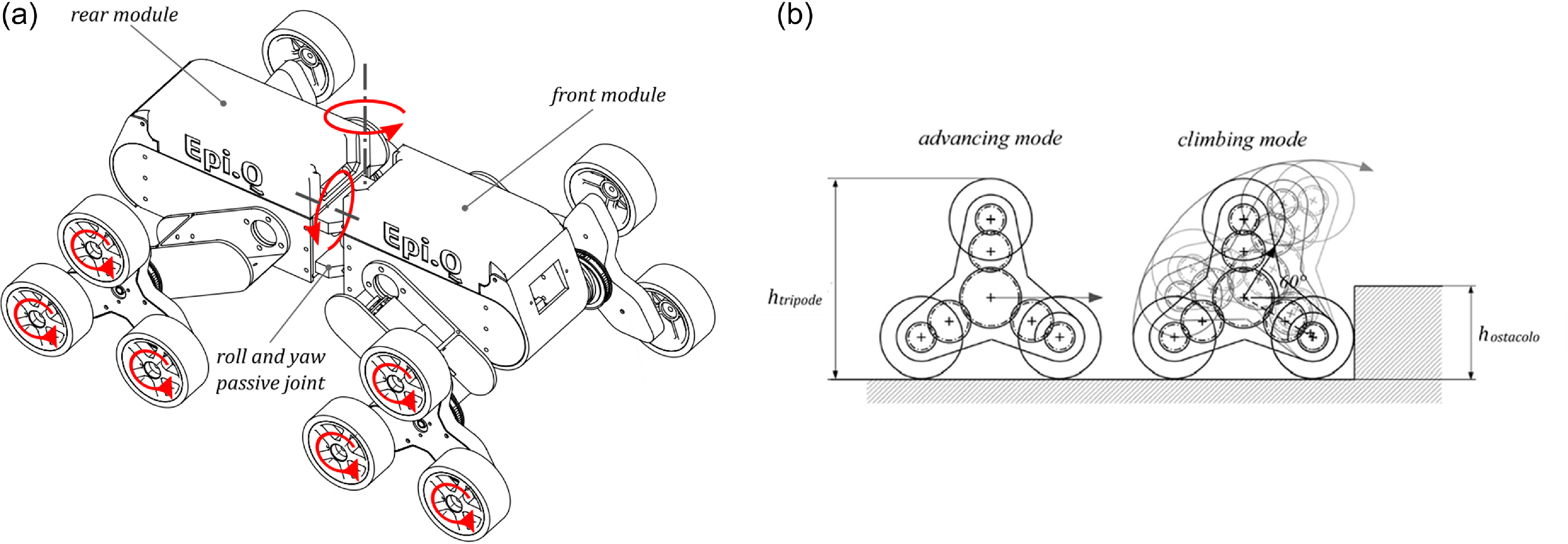
Epi.Q is based on a modular design consisting of two main frames, or modules, connected by a passive double rotary joint (Figure 1a). This joint allows for relative rotation in both roll and yaw, enabling Epi.Q to adjust its configuration to guarantee proper contact with the ground, thus enhancing navigation on unstructured terrain.
(a) The modular structure of the Epi.Q robot with a double rotary passive joint enabling roll and yaw rotation between modules, enhancing terrain adaptability. (b) Illustration of the tripod locomotion system that allows automatic mode-switching between advancing and climbing modes.

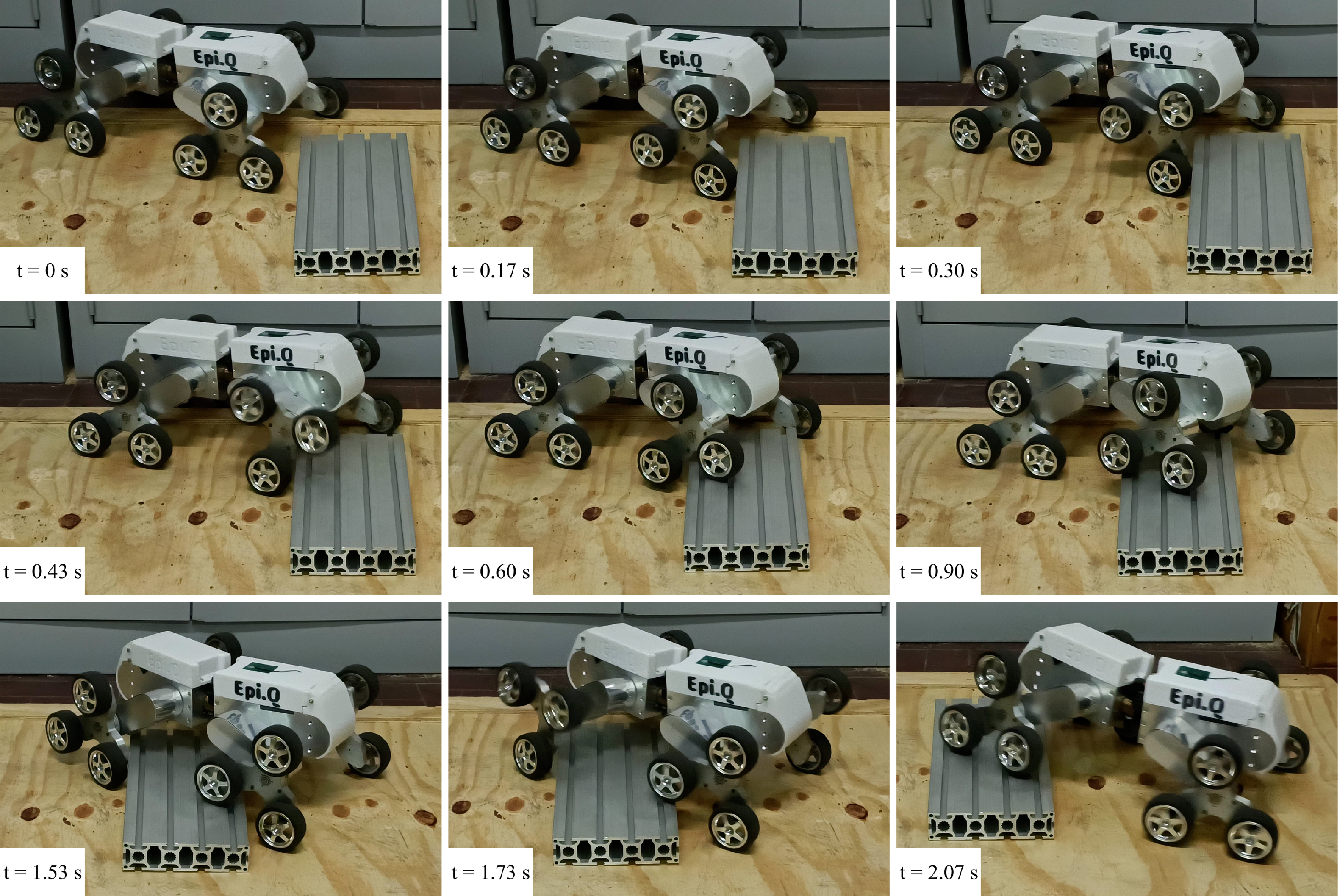
A defining feature of the Epi.Q is its tripod locomotion system. This system is based on an underactuated planetary gear mechanism that provides two distinct modes of operation: one for moving on the terrain (advancing mode) and another for overcoming obstacles (climbing mode). The transition between these modes is completely passive (Figure 1b), i.e., the robot automatically changes its locomotion strategy without requiring any active control input. This capability is particularly useful in unpredictable environments where the robot may encounter obstacles, as the system allows the robot to continue moving efficiently without interruption. As mentioned earlier, this motion is due to the epicyclic gear train inside the tripod: a motor drives the sun gear, while the tyres are fixed to the planetary gears, and the tripod itself is the carrier of the planet gears. When the tyres are not locked, the system acts as an ordinary gear train transmitting power from the sun gear to the plant gears, and thus the wheels. As soon as the tyres face significant resistance, the carrier, i.e., the tripod frame, rotates allowing for climbing obstacles while advancing. In Figure 2, a sequence of frames shows how the tripods passively switch between advancing and climbing modes while overcoming an obstacle.
Time-lapse sequence of the Epi.Q robot overcoming an obstacle, focusing on the switching of the tripods between advancing and climbing modes.

The Epi.q robot contains a number of essential electronic and electrical components. Its microcontroller, a Teensy 3.5 board, allows efficient data and command management. The robot’s motion is powered by four independent DC brush motors, each connected to a locomotion unit to allow the wheels to move independently. Wireless communication is managed by an XBee radio receiver, allowing remote commands to be received. A potentiometer on the joint between the modules measures the yaw angle, which is used in fuzzy control to improve stability. An external memory unit records real-time navigation data to aid in the analysis and validation of the control system.
3. Control strategy
The control strategy implemented for the Epi.Q robot is designed to address the complexities associated with its articulated structure and the skid-steer locomotion system, which make it particularly challenging to maintain stability, traction, and maneuverability in unpredictable environments such as uneven terrain and steep slopes. Due to its two independent modules connected by an articulated joint, the Epi.Q robot is susceptible to specific problems such as lateral slippage, loss of traction, and jackknife effects. Jackknife, which occurs when misalignment between the front and rear modules causes severe instability, is a major challenge because it can be difficult to realign the vehicle once it begins to deviate from the intended trajectory. In particular, the non-linearities arises from several structural and dynamic characteristics of the robot:
-
• The robot consists of two modules connected by a two-degree-of-freedom passive joint allowing relative rotation between the modules without actuation or control. This introduces complexity in modeling the coupling dynamics between the two bodies and requires significant attention to avoid unstable condition that could lead to jackifing or similar behaviors.
-
• Each module has a skid-steering architecture with two pairs of wheels in contact with the ground controlled by two motors, for a total of eight wheels and four motors. Skid-steering architectures inherently suffer from significant lateral slippage, heavily affecting the nonlinear tyre-ground contact dynamics and thus how much effective force can be exchanged with the ground without dissipating too much energy in wheel slipping.
-
• Each locomotion unit is made of an underactuated epicycloidal gearing where a single motor drives two degrees of freedom: the rotation of each wheel about its axis and the revolution of the whole tripod (and thus the wheels too) about its axis. Due to the underactuated nature of this mechanism, there is no way to directly control or select one of the two motion. Rather, the resulting movement will be given by the dynamic conditions of each locomotion unit. In particular, it is the complex dynamics of the contact between the wheels and the ground that governs how the drive torque is distributed to the degrees of freedom: a change in surface or wheel slip can lead to a sudden and undesirable rotation of the entire tripod, substantially modifying the robot’s motion.
-
• Both of the previous two points are directly influenced by wheel-ground contact dynamics. Contact models are already particularly complex in terms of identifying the parameters for conventional vehicles moving over typical non-deformable terrain. In this case, the situation is further complicated by dealing with a vehicle that potentially navigates through a broad spectrum of terrain, deformable and non-deformable and it is subject to high lateral slippage due to the skid-steering architecture. In addition, there is the added complexity of correctly modeling the forces exchanged on the ground by each wheel due to the torques applied to the rotation of the tripod and thus the increase and decrease of the normal force discharged by the wheels in contact with the ground. Since it is nontrivial to predict how much torque is transmitted to the tripod and how much to the wheels at each instant as internal friction and external conditions vary, it is extremely complex to model the normal contact forces and consequently the contact forces in general of each individual wheel.
The primary goal of the control strategy is to manage the robot’s motion by adjusting the power distribution between all the tripod units and ensuring that the vehicle follows the desired trajectory. This requires taking into account the complex coupled dynamics between the front and rear modules, as the articulation and presence of eight active wheels create interactions that must be carefully managed to prevent slippage and ensure smooth, reliable operation over dynamic and challenging terrain. Notably, this control approach was developed in the absence of a reliable dynamic model for the system, making it essential to employ alternative strategies to handle the nonlinear behavior and uncertainty inherent in the articulated structure of the Epi.Q.
The front module is primarily responsible for steering, so speed control is implemented, while the rear module provides additional power as needed. To manage the complex dynamics of the vehicle, especially in challenging environments, a fuzzy control system was implemented for the rear module. This choice of control method is particularly suitable for systems that must handle multiple inputs and nonlinear behavior, such as the articulated structure of the Epi.Q, without the need for a precise mathematical model.
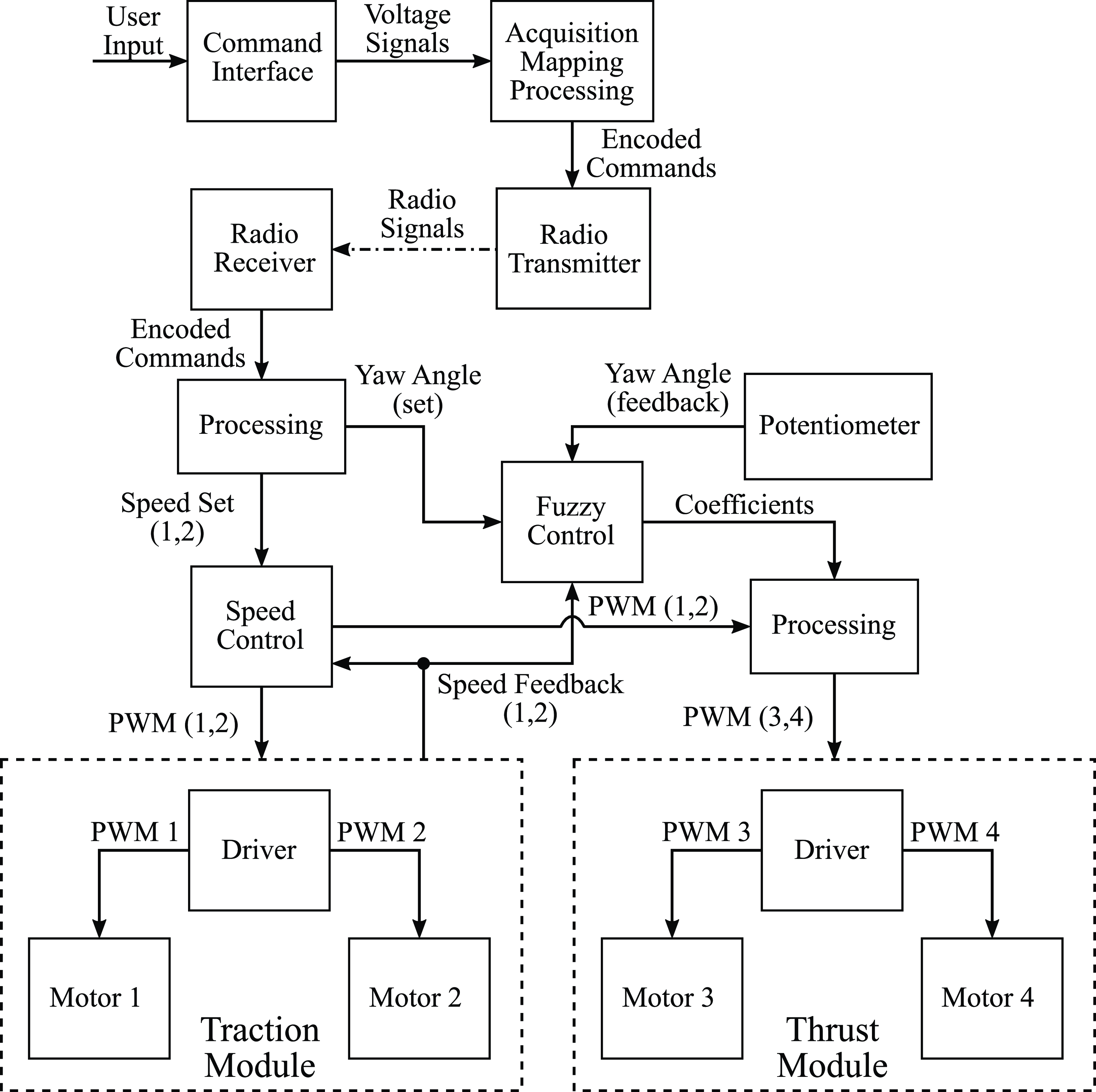
Block diagram of the control system featuring fuzzy logic for managing thrust module. The system processes user inputs, received via radio transmission, and generates PWM signals to control motors.

Figure 3 illustrates the control process. The robot is divided into two distinct modules: the traction module and the thrust module. This modular division facilitates the handling of reversal maneuvers, particularly due to the robot’s symmetrical design.
The traction module is speed controlled using a PID structure with anti-windup and feedforward functions. The anti-windup mechanism helps prevent excessive error accumulation in the integral component as the system reaches saturation, allowing for faster and more stable responses during transients. The feedforward function improves the dynamic response of the system by providing an open-loop command that reduces the load on the integral component, especially during transient phases.
The thrust module, controlled by a fuzzy control system, uses the yaw angular error and velocity feedback from the traction module as input. The angular setpoint is generated by processing user commands according to the robot’s kinematic model, which will be described later. The actual angle is measured by a potentiometer mounted on the joint.
The fuzzy control modulates the duty cycles of the thrust module by generating two multiplicative coefficients. The duty cycles determined by the speed control for the traction module are transferred to the thrust module and then multiplied by these two coefficients. In this way, the fuzzy control allows the thrust module to assist the traction module, taking into account the robot’s attitude and avoiding excessive thrusts that could cause jackknife phenomena.
To simplify the control and also easily manage the reverse, the control program differentiates between physical and logical modules. The logical modules are temporary and adjust based on the robot’s conditions and commands. The traction module is referred to as the ”Front” and the thrust module as the ”Rear”. These temporary modules are mapped to fixed physical modules, allowing the same type of control to be applied to both the traction and thrust systems, regardless of movement direction. This ensures no operational difference between forward and reverse motions.
By using a different nomenclature for the fixed physical modules, specifically ”M1” and ”M2,” it becomes easier to understand how the control logic operates. The ”Front” module is always speed controlled, while the ”Rear” module is managed using fuzzy control. When module M1 is assigned as the traction unit for the chosen forward direction, it functions as the ”Front” module, and the other module, M2, is automatically designated as the ”Rear”. When the direction of movement is reversed, the roles of the modules switch, making M2 the ”Front” and M1 the ”Rear”. By default, M1 is considered the front module. A distinguishing feature is that M2 is connected to the joint plates and the potentiometer body. This configuration works effectively because the robot’s design is symmetrical; otherwise, it could have caused operational issues. Assuming M1 is the front module, the four motors can be referred to as front left, front right, rear left, and rear right.
3.1. Simplified kinematic model
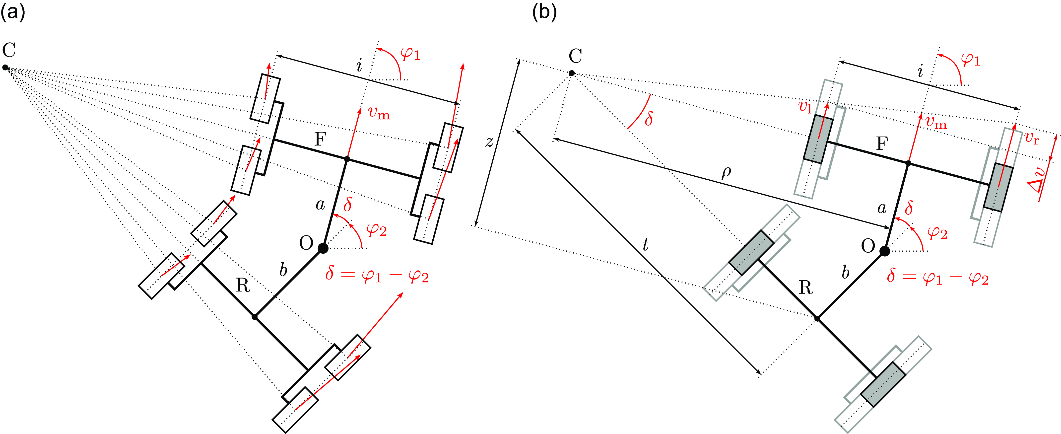
Unlike conventional cars, Epi.q is equipped with differential steering. This means that it can navigate a curve by imposing a difference in speed between the inner and outer wheels, rather than rotating them. In addition, as illustrated in Figure 4a, the presence of tripods causes lateral velocity components to be generated in curves. These lateral velocities tend to cause outward slipping and make the robot prone to understeering. The effect increases as the radius of the curve decreases.
Epi.Q kinematic model. (a) Real wheels with lateral velocity, showing potential for outward slipping during curves, which causes understeering. (b) Virtual wheels without lateral velocity, simplifying the model and eliminating slip during movement.

To simplify the kinematic model, each tripod is replaced by a virtual wheel (Figure 4b), which lacks lateral velocity components and thus does not slip. This modeling approach is derived from previous work, as discussed in [Reference Botta, Cavallone, Tagliavini, Carbonari, Visconte and Quaglia9]. Given the geometry of the robot, the radius of curvature of the front module
 $\rho$
is a function of the speeds imposed on the front wheels. Is it possible to define the front module angular velocity
 $\dot {\varphi }_1$
in two ways:
 \begin{gather*} \dot {\varphi }_1 = \frac {v_{\mathrm{m}}}{\rho } \\ \dot {\varphi }_1 = \frac {\Delta v}{i} \end{gather*}
where
 $\rho$
is the radius of curvature,
 $v_{\mathrm{m}}$
is the average velocity,
 $\Delta v$
is the difference in velocity between the inner and the outer wheelm and
 $i$
is the wheelbase. Consequently, the following relation can be derived:
 \begin{equation} \rho = \frac {v_{\mathrm{m}}}{\Delta v} \, i \end{equation}
There is a second relationship that relates the radius of curvature
 $\rho$
to the yaw angle
 $\delta$
. This relationship is valid only when conditions are stationary, meaning
 $\delta$
is constant. It is expressed as:
 \begin{gather*} z = a + b \cos {\delta } \\ t = \frac {z}{\sin {\delta }} \\ \rho = t \cos {\delta } + b \sin {\delta } \end{gather*}
from which we obtain:
 \begin{equation} \rho = \frac {a \cos {\delta + b}}{\sin {\delta }} \end{equation}
where
 $z$
and
 $t$
are the geometric distances visible in the Figure 4b,
 $a$
and
 $b$
are the distance from the yaw joint and the center between the wheels of the front module and the wheels of the rear module, respectively. By equating the relations 1 and 2, we obtain a third relation that relates linear velocities to yaw angles:
 \begin{equation} i \, v_{\mathrm{m}} \sin {\delta } = \Delta v (a \cos {\delta } + b) \end{equation}
By rewriting the equation as a function of the motors’ angular velocities, we get:
 \begin{equation} i \, n_{\mathrm{m}} \sin {\delta } = \Delta n (a \cos {\delta } + b) \end{equation}
Let
 $n_{\mathrm{l}}$
and
 $n_{\mathrm{r}}$
be the angular velocities (rpm) of the left and right motors, respectively, we can write that:
 \begin{gather*} n_{\mathrm{m}} = \frac {n_{\mathrm{r}} + n_{\mathrm{l}}}{2} \\ \Delta n = n_{\mathrm{r}} - n_{\mathrm{l}} \end{gather*}
Consequently, counterclockwise curves have both a positive
 $\Delta n$
and a positive angle
 $\delta$
(figure 4b). By substituting in the eq. 4 and performing a few steps, we obtain:
 \begin{equation} n_{\mathrm{r}} = n_{\mathrm{l}} \, \dfrac {1+\dfrac {i \sin {\delta }}{2(a \cos {\delta }+b)}}{1-\dfrac {i \sin {\delta }}{2(a \cos {\delta }+b)}} \end{equation}
Assuming:
 \begin{equation} K = \dfrac {1+\dfrac {i \sin {\delta }}{2(a \cos {\delta }+b)}}{1-\dfrac {i \sin {\delta }}{2(a \cos {\delta }+b)}} \end{equation}
equation 5 simplifies to:
 \begin{equation} \dfrac {n_{\mathrm{r}}}{n_{\mathrm{l}}} = K(\delta ) \end{equation}
which tells us that the ratio of the motor speeds is a function of the yaw angle and, through eq. 2, consequently a function of the radius of the curve we want to follow. From this point onward,
 $K$
is referred to as the coefficient of curvature. Equation 7 indicates that on a constant radius curve, the velocity relationship remains constant, regardless of speed, assuming no slippage. By introducing the average angular velocity, we can rewrite it as follows:
 \begin{equation} n_{\mathrm{r}} = \frac {2Kn_{\mathrm{m}}}{K+1} \end{equation}
The last equation can be used to calculate the speed of a single motor given the yaw angle
 $\delta$
and the speed of the module.
3.2. Rear control
The goal of rear module control is to enable the robot to have all-wheel drive, specifically eight wheel drive (8WD) in the case of Epi.Q. To achieve active control of the rear module, a fuzzy control system was implemented. This system takes into account both the yaw angular error and the robot’s instantaneous speed. It modulates PWM signals sent to the rear motors through the generation of two multiplicative coefficients to properly control them.
The angular error plays a crucial role since the yaw angle
 $\delta$
determines the robot’s steering behavior. Hence, it must be considered when executing control to maintain the correct robot configuration during movement. The angular reference is derived from the kinematic model based on the commands sent to the robot, while feedback is provided by a potentiometer mounted on the yaw joint. We can define the angular error as
 $e = \delta - \delta _{\mathrm{fb}}$
, where the angle is positive for counterclockwise turns.
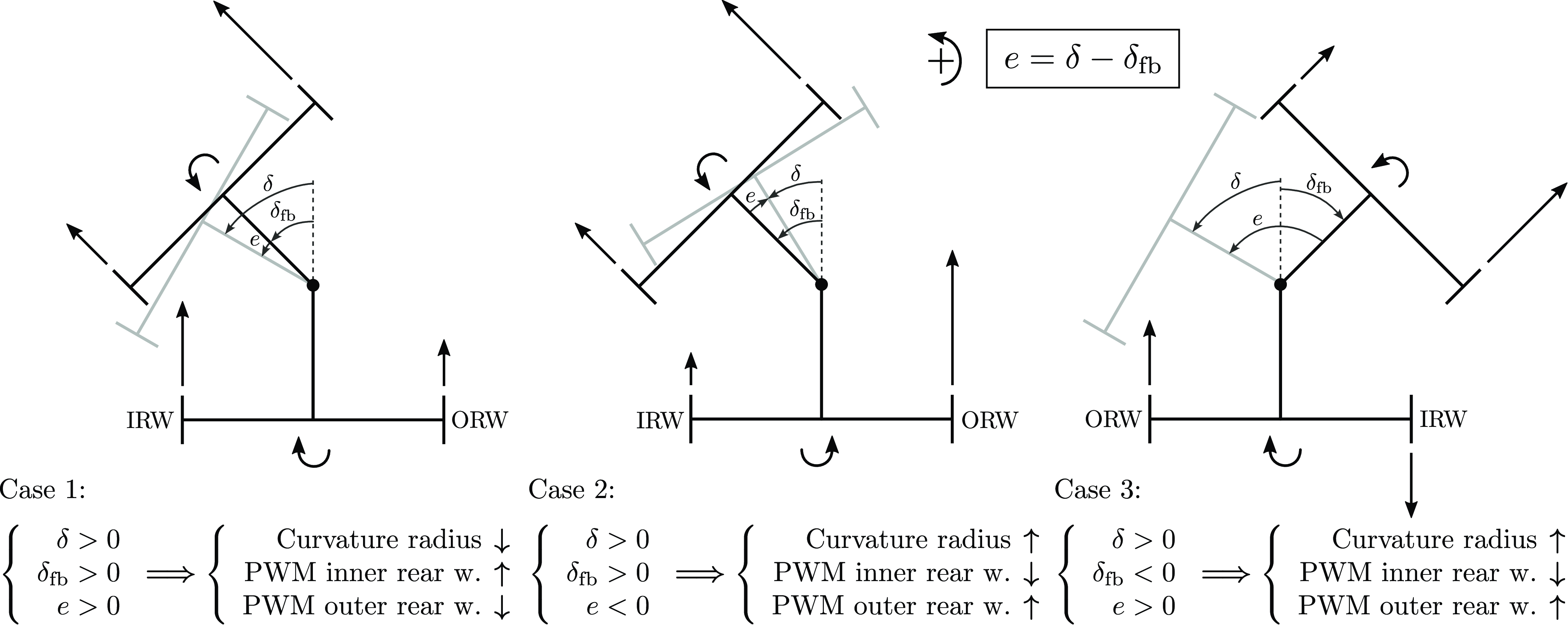
Figure 5 illustrates several generic movement configurations that the robot can assume. The straight arrows on the wheels represent the PWM command sent to each motor, while the circular arrows on the modules qualitatively indicate the rotation of the modules themselves. In the figure,
 $\delta$
is the desired yaw angle,
 $\delta _{\mathrm{fb}}$
is the feedback yaw angle, and
 $e$
is the error between them.
Diagram showing three steering cases for the vehicle dynamics, including adjustments for inner rear wheel (IRW) and outer rear wheel (ORW) based on the steering angle and feedback. PWM signals are adjusted to modify the curvature radius and correct steering errors in different cases.

Assuming that we have generated two PWM signals through the speed control for the front module, we can then determine how to modulate the command for the rear module. The base PWM signal is taken from the corresponding front motor. The left rear motor receives the PWM signal from the left front motor, and the same applies for the right side. We also define the rear wheels based on whether they are on the inside or outside of the curve. The inner rear wheel is referred to as IRW, and the outer rear wheel as ORW, based on the sign of the measured yaw angle
 $\delta _{\mathrm{fb}}$
.
There are six possible cases, but given the system’s symmetry, we only show three, with the others being mirror images along the vertical axis, where all angle signs and errors are inverted. However, the corrective actions remain the same.
In Case 1, the robot is navigating a counterclockwise curve, but the measured angle is smaller than the target, meaning
 $\delta \gt \delta _{\mathrm{fb}}$
. To restore the correct configuration and reduce the turning radius, we adjust the rear module’s signals by increasing the PWM on the inner rear wheel and decreasing it on the outer rear wheel, helping the rear module to tighten the robot’s turn and increase
 $\delta _{\mathrm{fb}}$
.
In Case 2, the situation is similar, but
 $\delta _{\mathrm{fb}} \gt \delta$
, so the corrective actions are inverted, as the goal here is to increase the turning radius.
In Case 3, the robot is navigating a clockwise curve but receives a command for a counterclockwise one. Speed control generates PWM for the front module, which gradually aligns with the final configuration. To accelerate this transition, the inner rear wheel is used as a brake until the robot returns to the configuration described in Case 1.
3.3. Fuzzy control
The fuzzy control logic is based on a mathematical-logical theory that introduces the concept of the gradual membership of an element to a set. Unlike traditional logic, which handles events as either true or false, fuzzy logic allows for representing a continuous range of values, providing a more flexible and realistic representation for managing complex and nonlinear systems, such as Epi.Q. This type of control is especially suitable for handling systems with multiple inputs, as it allows defining various behaviors depending on operating conditions [Reference Lee24–Reference Zimmermann28].
A typical fuzzy control system consists of three main modules: the fuzzification module, the rule application module, and the defuzzification module. Both inputs and outputs are specified by numerical (crisp) values, while the fuzzy controller operates on fuzzy variables. Thus, there are fuzzification and defuzzification interfaces, which associate inputs with their fuzzy representation and convert the fuzzy output back into crisp values. The central rule application transforms the fuzzy representations of the inputs into fuzzy output representations according to fuzzy logic rules, also known as inference rules. The defuzzification process then converts these fuzzy values back into crisp signals for output.
Fuzzification, or the conversion into fuzzy variables, is carried out through membership functions (
 $\mu$
), which define the degree of activation of a class. These functions can take various forms; common examples include triangular, trapezoidal, piecewise linear, or Gaussian functions. In our implementation, we chose to use triangular and trapezoidal membership functions for both inputs and outputs.
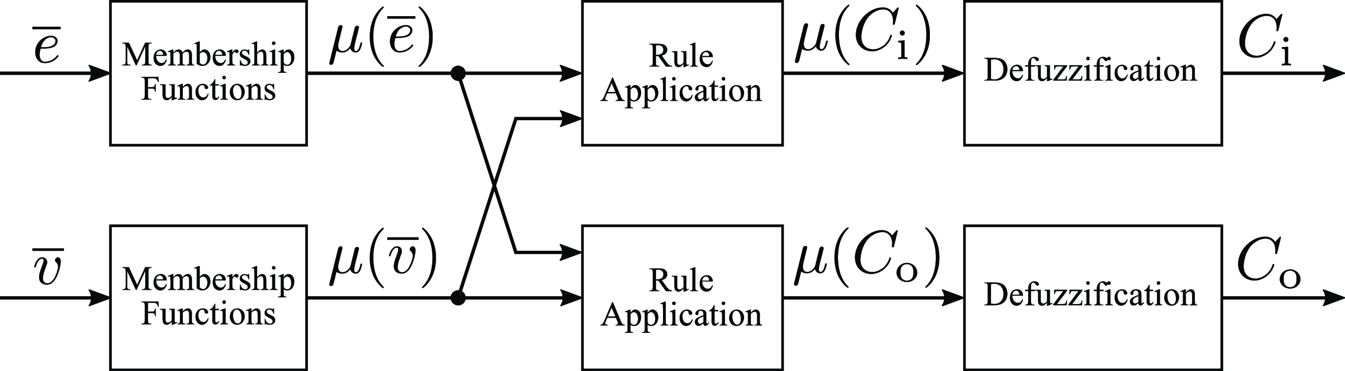
Fuzzy control system for Epi.Q robot. Inputs include normalized angular error and speed, while outputs modulate the duty cycle applied to the inner and outer rear wheels.

Figure 6 presents the fuzzy control scheme implemented on the Epi.Q robot. The inputs are the normalized angular error (
 $\overline {\mathit{e}}$
) and the normalized average speed (
 $\overline {\mathit{v}}$
), defined as follows:
 \begin{align}& \overline {e} = \mathrm{sign}(\delta _{\mathrm{fb}})\,\frac {\delta - \delta _{\mathrm{fb}}}{\delta _{\mathrm{max}}} \end{align}
 \begin{align}&\quad\,\, \overline {v} = \left \lvert \frac {n_{\mathrm{r}} + n_{\mathrm{l}}}{2\,n_{\mathrm{max}}}\right \rvert \end{align}
where
 $\delta$
is the set yaw angle imposed by the control logic,
 $\delta _{\mathrm{fb}}$
is the feedback yaw angle measured by the potentiometer, and
 $\delta _{\mathrm{max}}$
is the maximum angle the robot can reach before the joint hits its mechanical stop, equal to 38
 $^\circ$
. The yaw angle is therefore confined to the range [−38
 $^\circ$
, 38
 $^\circ$
], while the normalized error (
 $\overline {\mathit{e}}$
) is defined in the range [−2, 2].
In the second equation,
 $n_{\mathrm{r}}$
and
 $n_{\mathrm{l}}$
are the angular velocities of the front motors, which are speed controlled. The term
 $n_{\mathrm{max}}$
represents the maximum angular velocity, which is 10 000 rpm. Considering the gear ratio, the tripod mechanism, and the wheel diameter, the maximum linear velocity of the robot is 2.68 m/s.
The fuzzy control output consists of two multiplicative coefficients that modulate the duty cycle applied to the motors. The coefficient
 $C_{\mathrm{i}}$
modulates the inner rear wheel, while the coefficient
 $C_{\mathrm{o}}$
modulates the outer rear wheel.
 $C_{\mathrm{i}}$
varies in the range [−0.8, 1.4], and
 $C_{\mathrm{o}}$
varies in the range [0.4, 1.4]. Negative values indicate a torque inversion by the motor to perform braking or even reverse.
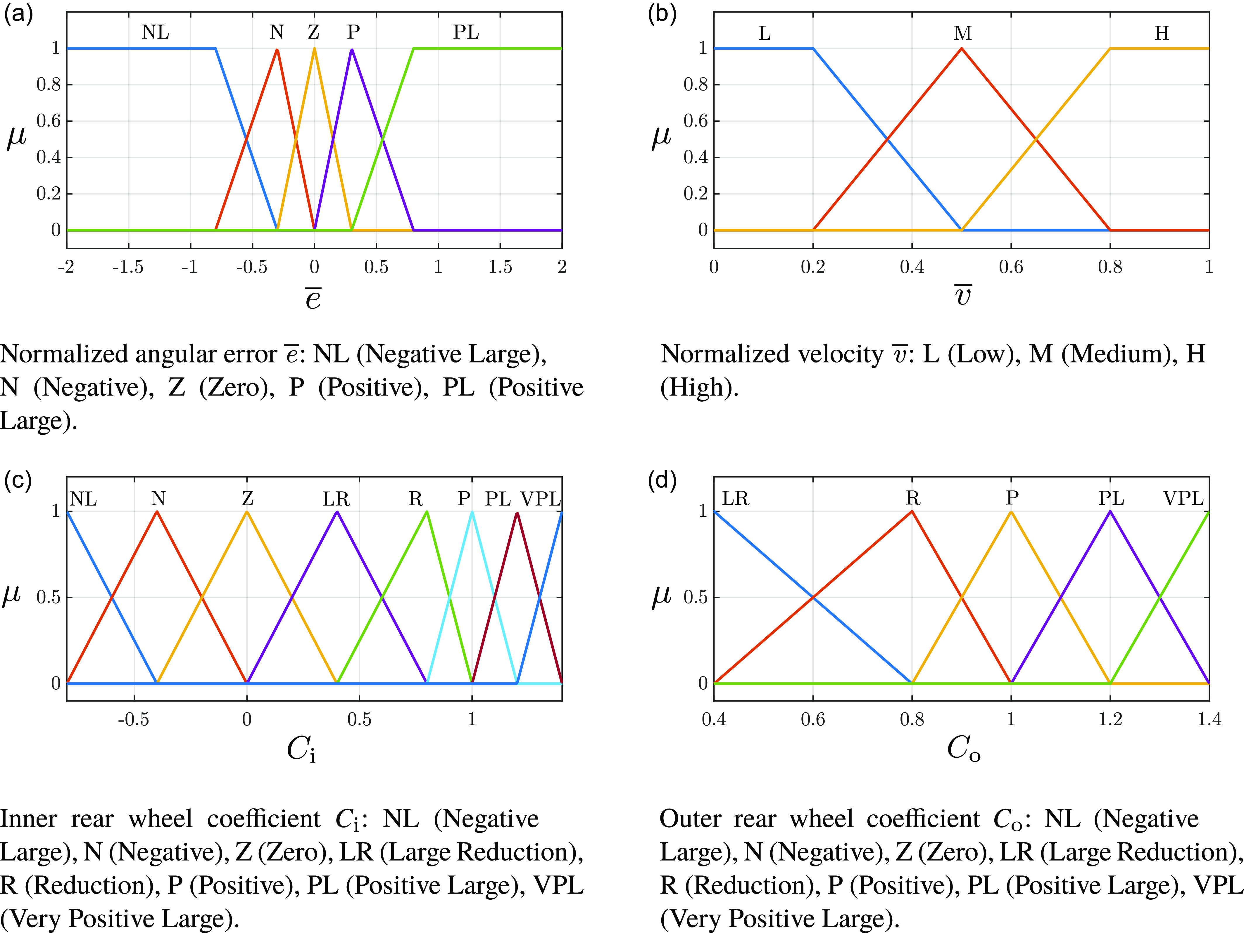
Membership functions for the fuzzy control system inputs (
 $\overline {\mathit{e}}$
,
 $\overline {\mathit{v}}$
) and outputs (
 $C_{\mathrm{i}}$
,
 $C_{\mathrm{o}}$
).

The membership functions of the two input variables and the two output variables in the fuzzy system are shown in Figure 7. The x-axis indicates the numerical value of each variable, while the y-axis indicates the degree of membership to each class. Specifically, the normalized error
 $\overline {\mathit{e}}$
(Figure 7a) is divided into five classes. Two flat regions are included to ensure full coverage of the input domain, although in most operational cases, the controller functions within a reduced range, approximately [−1,1]. The normalized velocity (Figure 7b) is divided into three classes, again with flat regions at the boundaries. Figs. 7c and 7d displays the membership classes of the outputs. The outer rear wheel coefficient (
 $C_{\mathrm{o}}$
) has five membership classes, while the inner rear wheel coefficient (
 $C_{\mathrm{i}}$
) extends these by adding three additional classes to allow for negative values.
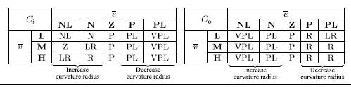
Fuzzy control involves writing rules in the form of IF (condition) THEN (action). This means that if a certain input is activated, the corresponding output is activated according to the rules. The simplest way to visualize these rules is through a matrix, called the rule matrix, which associates an output class with every pair of input classes. Since there are two distinct outputs, two separate matrices are created. In Table I, the rules on the left side aim to increase the curvature radius of the trajectory, while the rules on the right aim to decrease it.
Fuzzy control rule matrix used to modulate the duty cycle coefficients of the rear wheels of the Epi.Q robot. The rules are defined based on the angular error (
 $\overline {\mathit{e}}$
) and the robot’s velocity (
 $\overline {\mathit{v}}$
), allowing dynamic adjustments to enhance stability and precision during maneuvering and steering phases.

Lastly, it is worth noting that the speed-dependent component of the fuzzy control becomes particularly relevant for the inner rear wheel coefficient
 $C_{\mathrm{i}}$
, especially in scenarios involving negative normalized errors. Under these conditions,
 $C_{\mathrm{i}}$
is adjusted to contribute to increasing the curvature radius of the trajectory, allowing the vehicle to realign more effectively during high-curvature maneuvers.
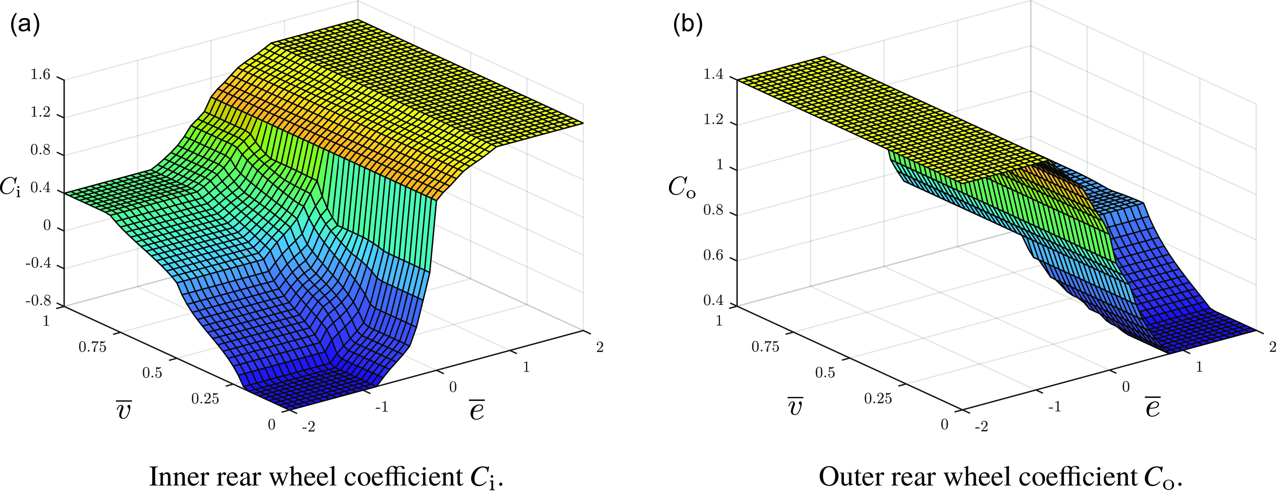
Fuzzy inference surfaces for the rear wheel coefficients.

Figures 8a and 8b shows the inference surfaces generated by the fuzzy control based on the rule matrices for the coefficients
 $C_{\mathrm{i}}$
and
 $C_{\mathrm{o}}$
, respectively. As can be seen, there is more aggressive control for low-speed values around zero error, and smoother control for higher speed values. This was necessary because at low speeds, the robot is much less sensitive to command variations.
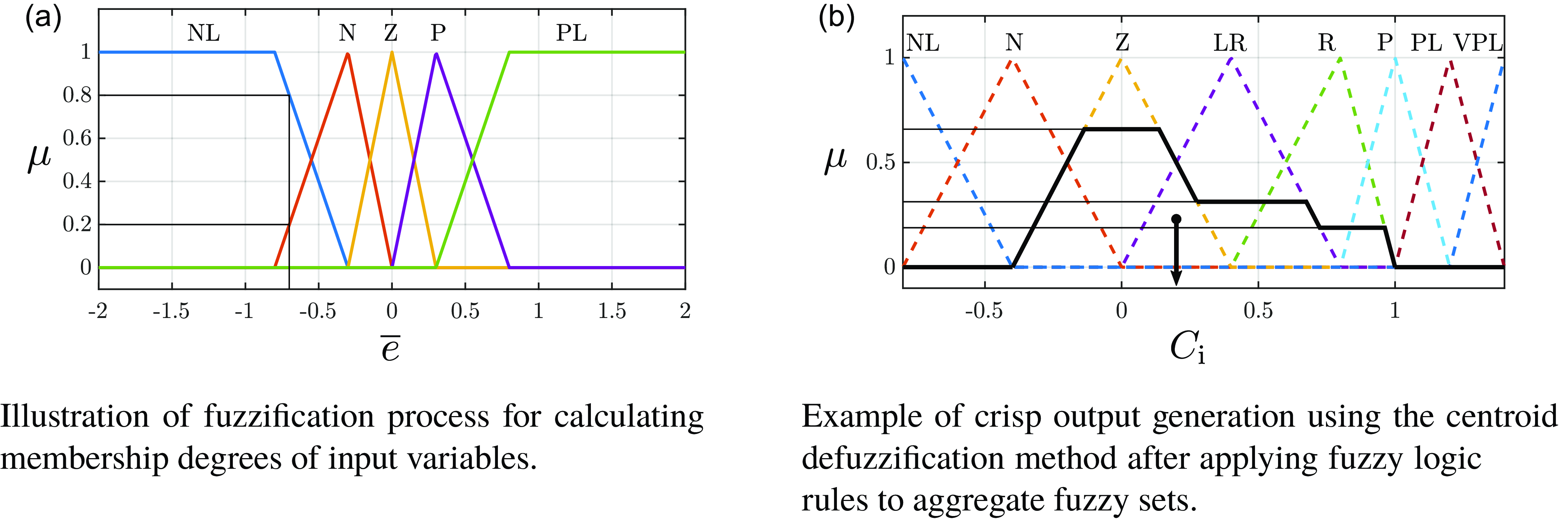
The inference method used for calculating output values is Mamdani’s method, which involves the following steps. Initially, the degrees of activation for the input variable classes are calculated (as shown in Figure 9a for the membership classes of the variable
 $\overline {\mathit{e}}$
). For each input value, one or two classes can be activated. The next step is to calculate the premise values (
 $\mu _{\mathrm{p}}$
), which is the intersection of fuzzy sets, according to the following formula:
 \begin{equation} \mu _{\mathrm{p}}(\overline {e}_i,\, \overline {v}_j) = \min (\mu _i(\overline {e}),\, \mu _j(\overline {v})) \end{equation}
Where
 $i$
and
 $j$
are the membership classes of the inputs. These premise values are used to define, based on the rule matrix, the activation degree of the output classes for each pair of input classes. Once the rule matrix is filled with the premise values, a fuzzy set union operation is applied, using the following formula:
 \begin{equation} \mu (u_k) = \max (\mu _{\mathrm{p}}(\overline {e_i},\,\overline {v_j})) = \max [\min (\mu _i(\overline {e}),\,\mu _j(\overline {v}))] \end{equation}
where
 $u$
represents a generic output, and
 $k$
indicates the membership class of the output.
Examples of fuzzification and defuzzification used in the proposed control.

After calculating the activation values of the output classes, a clipping (or alpha-cut) operation is performed, which ”cuts” the fuzzy membership function at a specific activation level (
 $\alpha$
), representing the maximum membership degree achieved by the active fuzzy rules. The result is a simplified fuzzy function, which can be further processed to obtain a crisp value. An alternative method is scaling, which proportionally resizes the membership function to the activation degree obtained from fuzzy inference, maintaining the shape of the original membership function.
The first method (clipping) is the most common due to its simplicity, offering high computational speed and simplifying the defuzzification process. The downside is that some information is lost during the clipping operation, as the shape of the function changes. For example, a triangular function becomes trapezoidal after clipping.
The second method (scaling), though computationally more expensive, allows adjusting the influence of a fuzzy rule on the output without losing information about the original membership function distribution. Unlike clipping, which removes parts of the function, scaling preserves all characteristics of the fuzzy curve, only reducing its intensity proportionally to the degree of activation.
At this point, the aggregation of the results is carried out to obtain a single fuzzy set for the output variable. Figure 9b shows an example where a single fuzzy set is obtained from the class aggregation after applying the alpha-cut method.
Defuzzification converts the fuzzy set output into a numerical (crisp) value. This conversion can be performed using several defuzzification methods, which associate a deterministic value with the fuzzy representation of the output. The method used here is the center of gravity method, one of the most commonly used due to its accuracy. It calculates the center of gravity of the resulting fuzzy set, and the output is the x-coordinate of that point, as shown in Figure 9b.
The choice of the Mamdani inference method for the fuzzification process was primarily motivated by its interpretability and accessibility. Mamdani-type systems use linguistic labels for both inputs and outputs [Reference Mamdani and Assilian29], making them particularly suitable for implementing expert knowledge, even from domain experts without a strong background in mathematics or control theory. This approach facilitates the development of intuitive fuzzy rule bases that can be easily modified and extended based on observed behavior and experiential knowledge [Reference Lee24, Reference Lee30].
While the Sugeno method is often preferred in scenarios requiring computational efficiency and mathematical precision, particularly when the system can be effectively described using analytical functions [Reference Sugeno31–Reference Blej and Azizi33], its reliance on numerical outputs makes it less intuitive for designing interpretable rule sets involving qualitative reasoning. In contrast, the Mamdani approach provides a more descriptive framework that aligns with the main objective of this work: developing a human-readable and easily adaptable control strategy for the highly non-linear and articulated structure of the Epi.Q robot. The ability to define both inputs and outputs using linguistic variables proved essential to integrating domain knowledge and simplifying the tuning process during prototyping and experimentation.
For defuzzification, the centroid method was chosen because of its high accuracy and ability to produce smooth and stable output signals. Although this method is generally more computationally intensive than alternative defuzzification techniques, such as mean of maxima or height methods, the centroid method ensures continuous and consistent control transitions [Reference Lee30], which is especially important for an articulated system like Epi.Q operating in unstructured terrain. The controller efficiently manages the associated computational load without compromising real-time responsiveness due to the relatively low update rate required for vehicle-level control and the moderate complexity of the fuzzy rule set. As a result, the additional computational load introduced by the centroid method is well within the capabilities of the on-board processing hardware and does not compromise performance or reliability.
The objective of this study is not to demonstrate the superiority of fuzzy logic control over more commonly adopted methods such as MPC or SMC. In fact, we explicitly do not attempt a direct performance comparison with these techniques. Such methods require a reliable dynamic model of the system, and a model is currently unavailable for Epi.Q due to its complex and nonlinear behavior, which is introduced by its articulated structure, passive joint dynamics, and unpredictable terrain interactions. Without a reliable model, MPC and SMC strategies would operate under inaccurate assumptions, making any comparison unfair or misleading.
Instead, fuzzy logic is proposed here as a pragmatic and feasible alternative designed specifically to bypass the need for a precise model. The aim is to improve traction and maneuverability in real-world environments with uncertainties, not to outperform state-of-the-art methods in idealized conditions. Thus, the contribution of this work lies in demonstrating a functional and practical control implementation that enhances robot behavior in scenarios where traditional model-based approaches are difficult or impossible to deploy.
3.4. System scalability and operational robustness
The current fuzzy logic control system is designed for a modular robot composed of two articulated modules, with control rules tailored to this specific configuration. Although the system is not inherently scalable, it can be extended to accommodate additional articulated joints or modules by incorporating new input variables and expanding the rule base accordingly. However, such a modification would significantly increase both the complexity of the control logic and the computational resources required to manage the expanded system dynamics. Careful optimization and modular rule design would be necessary to maintain system performance and real-time responsiveness.
From a hardware perspective, the Epi.Q robot is equipped with four motors, each integrated with a high-reliability Hall effect encoder for accurate motor speed feedback. These encoders are known for their durability and robustness against environmental disturbances, ensuring consistent performance over extended operational periods. The robot yaw angle is measured using a high-quality conductive plastic potentiometer, selected for its environmental resistance and durability despite the use of sliding contacts.
Robustness is further enhanced by the system’s ability to tolerate partial hardware failures. In the event of a motor failure, the robot is capable of operating in a 4WD mode, where either module can assume the role of the front (driving) module. Although this mode limits the robot’s ability to perform reverse maneuvers, it preserves forward mobility, allowing the robot to maintain basic functionality and perform mission critical tasks.
This combination of scalable control architecture and resilient hardware design enables the system to operate reliably under varying conditions while providing a basis for future extensions in both complexity and capability.
4. Preliminary tests
Before proceeding with the full-scale validation of the proposed control strategies for the Epi.Q robot, a series of preliminary tests were carried out to assess the basic capabilities and performance of the robot under different conditions. These tests focus on evaluating the robot’s locomotion and traction control system, with particular emphasis on scenarios that reflect typical operational environments. The tests are designed to verify the efficacy of the fuzzy logic control system and its contribution to the overall performance of the robot in tasks such as climbing, obstacle overcoming, steering, and starting from a misaligned position. The key objectives of these tests are to:
-
• Assess the robot’s climbing ability under various inclination angles.
-
• Evaluate the obstacle-overcoming capabilities of the robot.
-
• Analyze the robot’s steering behavior and realignment efficiency.
-
• Measure the time and precision required for the robot to regain alignment after a standing start.
The results of these preliminary tests will provide crucial insights into the system’s limitations and inform further refinements of the control strategy.
4.1. Uphill tests
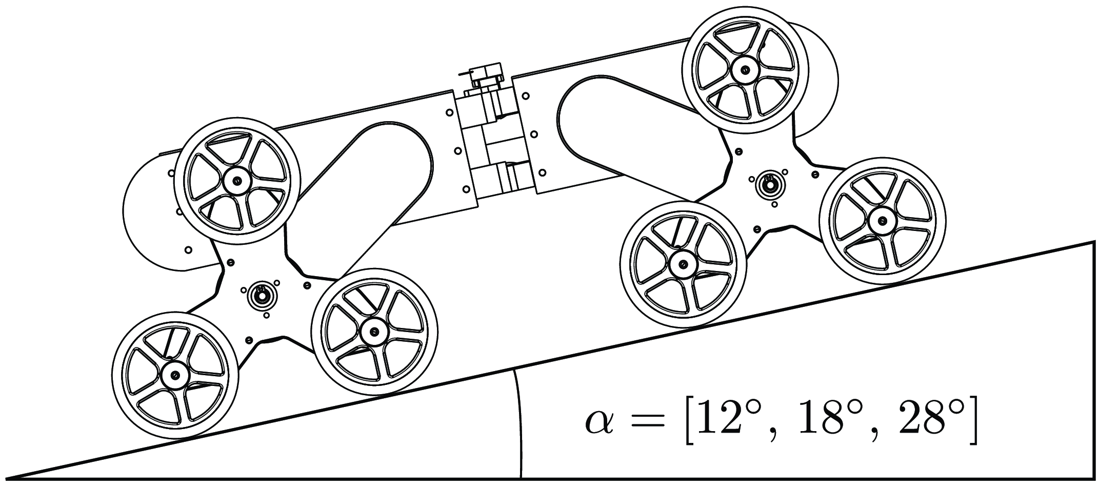
Figure 10 shows the setup of the test. The robot is placed on a flat wooden board whose inclination is varied. The tests were performed by imposing a speed set of 1200 rpm (0.32 m/s), with tilt angles of 12
 $^\circ$
, 18
 $^\circ$
, and 28
 $^\circ$
. The purpose of the test is to verify the climbing ability of the robot in the two different configurations (4WD and 8WD) and to demonstrate how much the use of the rear end affects its ability to cope with steep climbs.
In this first test, with an inclination of 12
 $^\circ$
, we compare the robot’s climbing ability with active fuzzy control and with only the front end.
Diagram illustrating the setup of the uphill test. The robot is placed on a flat wooden board with adjustable inclination, used to test the climbing ability of the robot in different drive configurations (4WD and 8WD) at varying angles of incline.

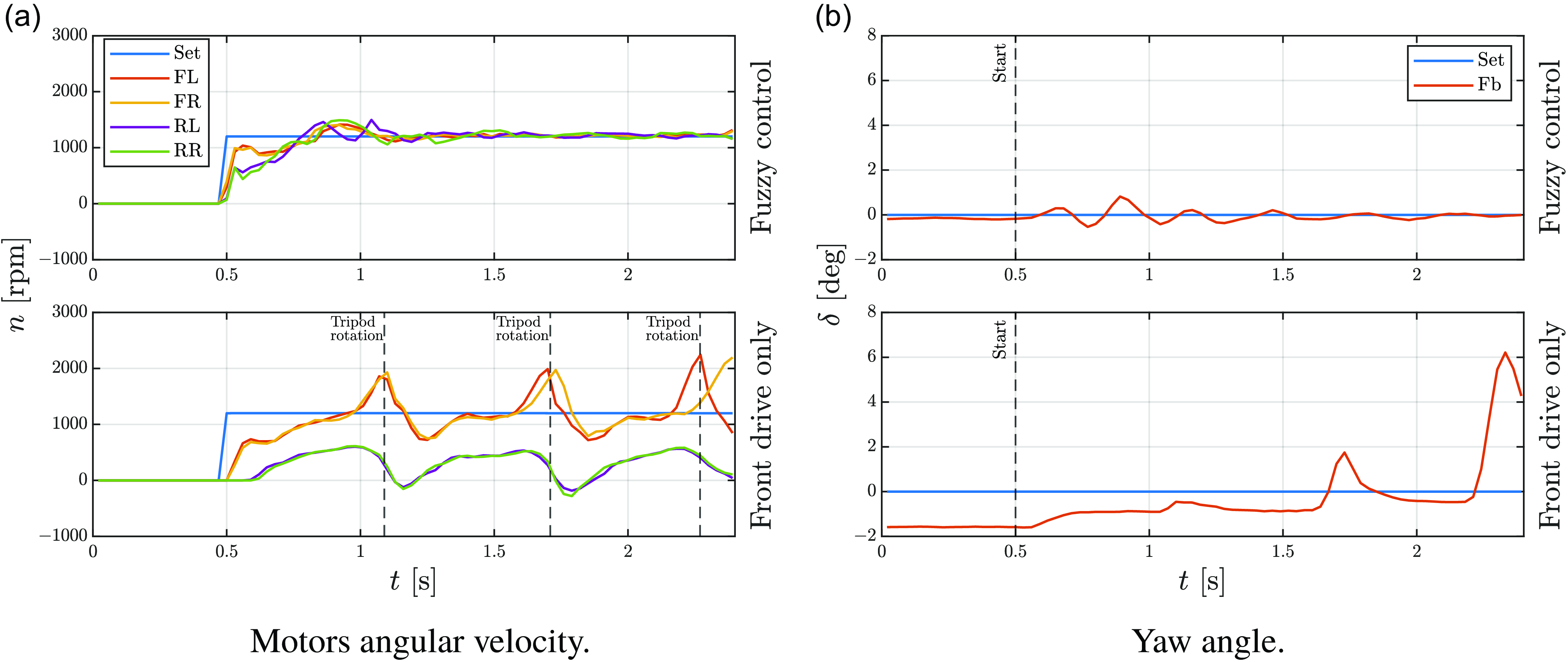
Uphill test,
 $\alpha = 12^\circ$
. Tripod rotations occur due to the high torque applied by the motors and the low normal load on the tripods themselves. With all-wheel drive, less torque is applied to the front tripods.

Figure 11a shows the graph of the speed of the motors. As can be seen, in 4WD mode, the robot is not able to achieve convergence in the speeds of all the motors. While the front tripods oscillate around the target speed, the rear tripods do not reach the target speed. In this mode, the rear motors are not powered, but they are connected to the wheels, so we can read the real speed of the robot.
In “Front drive only” (FDO) case, the tripods change from advancing mode to climbing mode, making them rotate without the tires transferring power to the ground. This happens because the vertical force needed to stop the tripods from rotating isn’t strong enough to balance the torque from the motors. As a result, Epi.Q cannot climb a ramp with such a slope. On the other hand, using 8WD mode and Fuzzy control, Epi.Q is able to climb this slope easily. It takes about 0.75 s to reach target speed.
Figure 11b illustrates the yaw angle during the test. In the FDO case, it is unstable, whereas with fuzzy control, it oscillates around the set value and and reaches the target after the acceleration phase.
Uphill test,
 $\alpha = [18^\circ ,\,28^\circ ]$
. Increasing the tilt angle causes the tripods to rotate due to the low normal load on the front tripods.

Since the robot with only the front module is not able to climb a slope with an inclination angle of 12 degrees, the next tests will be performed in 8WD mode with the fuzzy control active, in order to find out what is the maximum inclination angle the robot can handle.
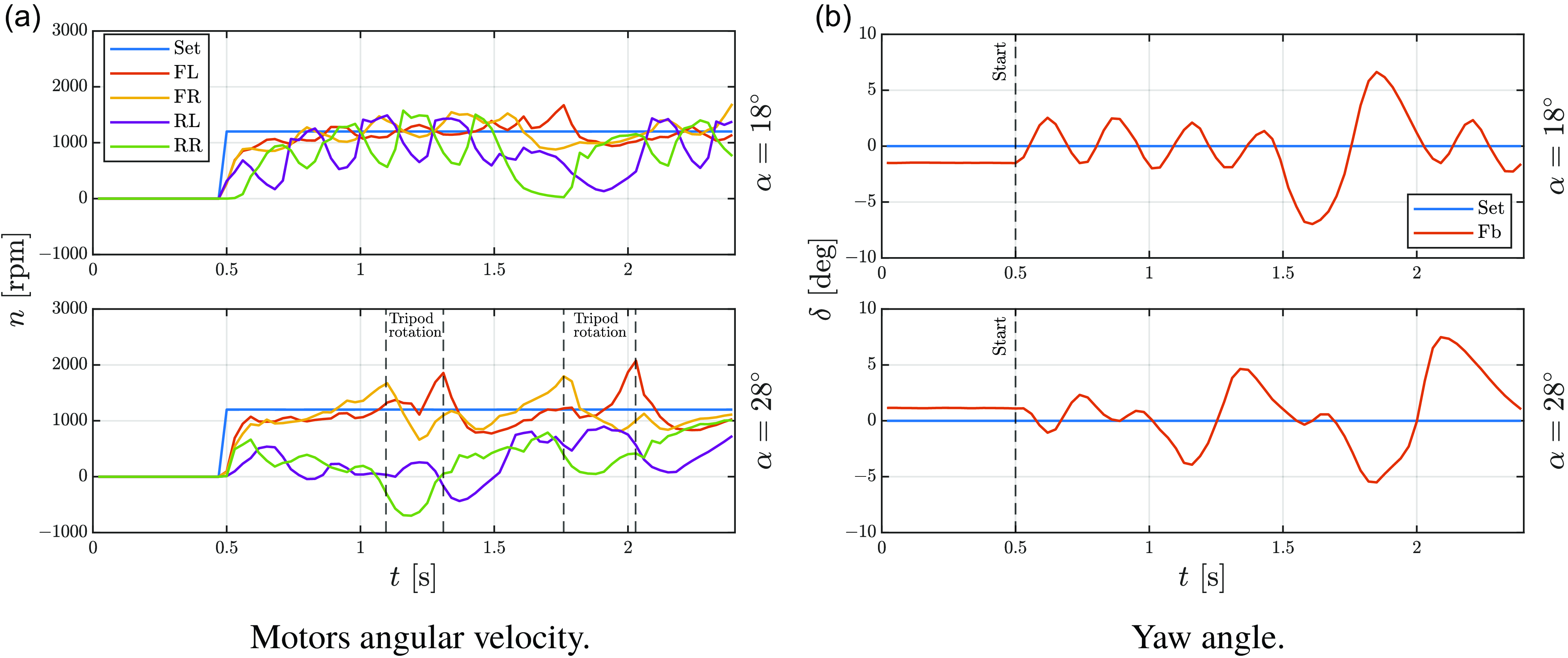
Figures 12a and 12b shows two tests performed with a tilt angle of
 $18^\circ$
and
 $28^\circ$
. In the first case (
 $\alpha = 18^\circ$
), the robot is able to climb the slope, but there is a lot of correction on the rear module to keep the alignment, as can be seen from the yaw angle graph and the speed graph. On such a slope, the front module’s tripods tend to rotate, but the wheels don’t switch completely.
In the second case (
 $\alpha = 28^\circ$
), the robot cannot go up the slope because the tripods of the front module switch from advancing mode to climbing mode due to the reduction of vertical load. As a result, the speeds measured by the rear module are much lower than the target speed.
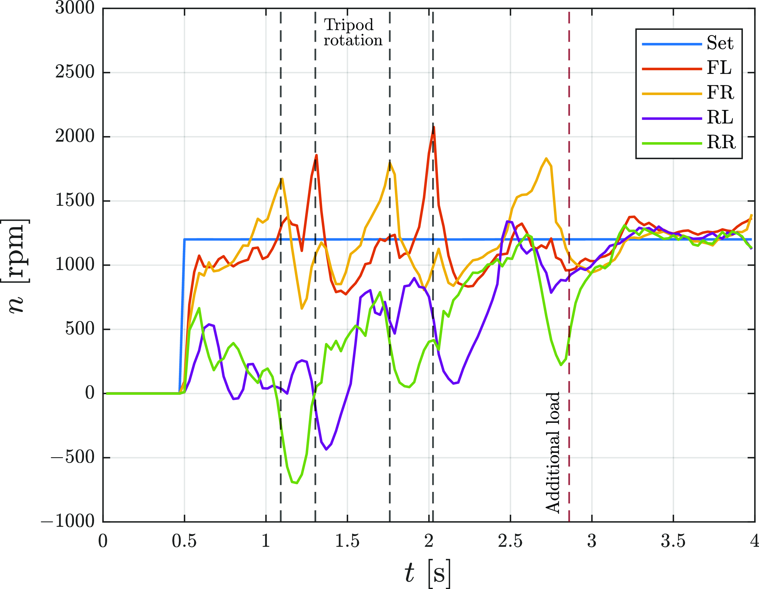
Uphill test with additional load,
 $\alpha = 28^\circ$
: motors angular velocity. The additional load prevents the tripod from rotating and allows the robot to climb.

In Figure 13, we continued the test with a tilt angle of 28
 $^\circ$
by applying an additional load to the robot’s front module so that there was a greater constraint on tripod rotation. As a result, Epi.Q can climb the slope in advancing mode.
4.2. Obstacle climbing
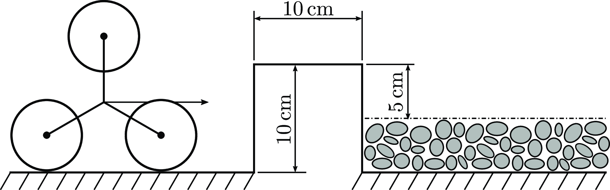
In the obstacle climbing test (Figure 14), the robot starts on a flat concrete surface, moves forward to the step, overcomes it, and travels a short distance on gravel. After that, it reverses direction and follows the same path back to its starting position. In the diagram, the tripod is shown to scale with the step.
Diagram of the obstacle climbing test. The robot starts on a flat concrete surface, approaches and climbs a step, and then moves onto gravel. It reverses the same path to test the robot’s ability to overcome obstacles in 8WD mode with fuzzy control.

The purpose of the test is to verify the robot’s obstacle-overcoming capability in 8WD mode with fuzzy control enabled. In 4WD mode, this specific test fails because once the front module passes the obstacle, it is unable to pull the rear module along.
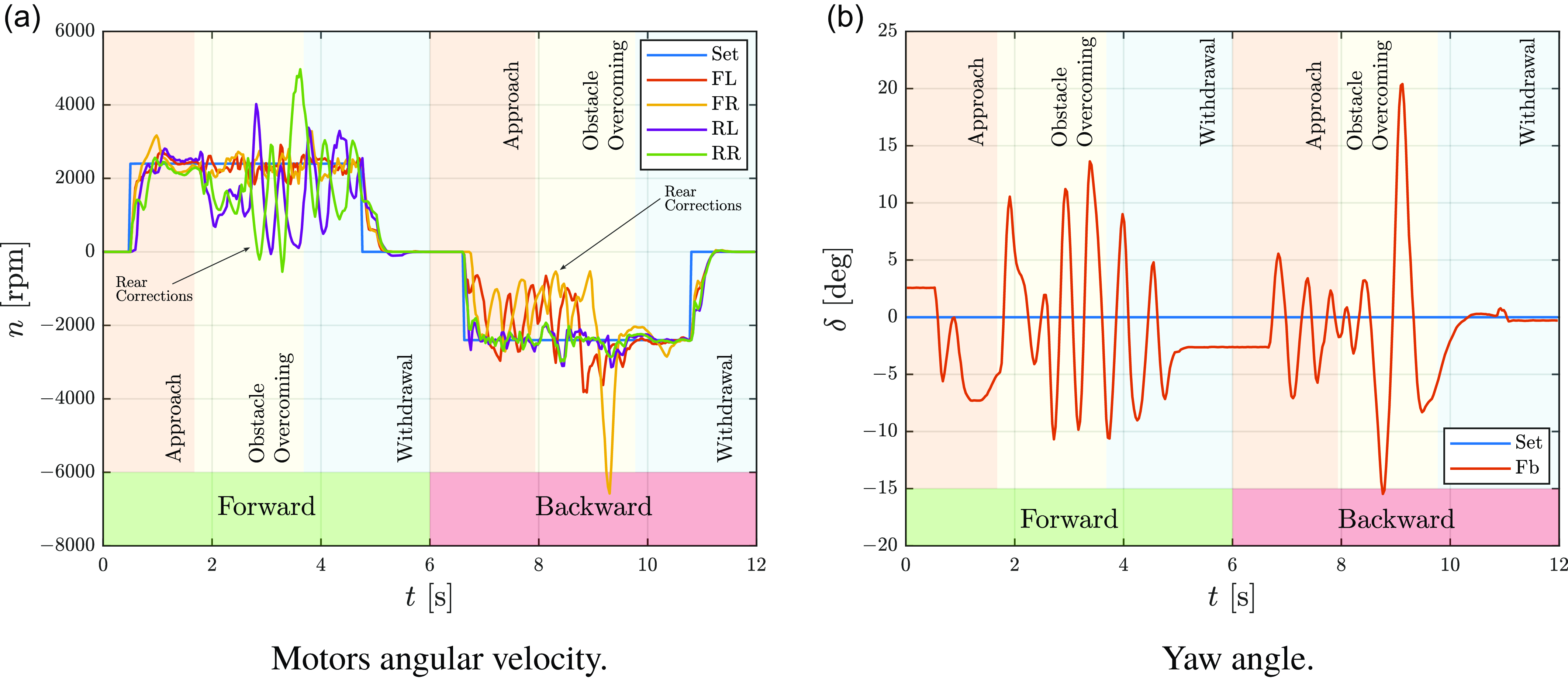
Figures 15a and 15b show the angular velocity of the motors and the yaw angle measured at the articulated joint, respectively. The test is divided into two parts: forward climbing and backward climbing. Each part is divided into three distinct phases: approaching the obstacle, overcoming the obstacle, and withdrawing from the obstacle. The overcoming phase begins when the front module’s wheels hit the obstacle and ends when the rear module is entirely on the gravel. The same thing happens in the backward phase but the modules are reversed.Footnote 1
Considering the forward overcoming, we can observe the transition between the approach phase and the overcoming phase. Once the front module hits the step, the tripods switch from advancing mode to climbing mode while maintaining the same angular speed of the motors (FL, FR). On the contrary, in the rear module, there is a noticeable drop in speed. During the overcoming phase, numerous corrections are made to the rear module to follow the target yaw angle. These corrections continue into the withdrawal phase due to the loose and uneven ground after the obstacle. In the backward motion, the pattern is the same but reversed, with the rear module controlled by velocity and the front by fuzzy.
Obstacle climbing test. Fuzzy control actively works to maintain rear alignment when climbing obstacles and on gravel surfaces.

4.3. Steering test
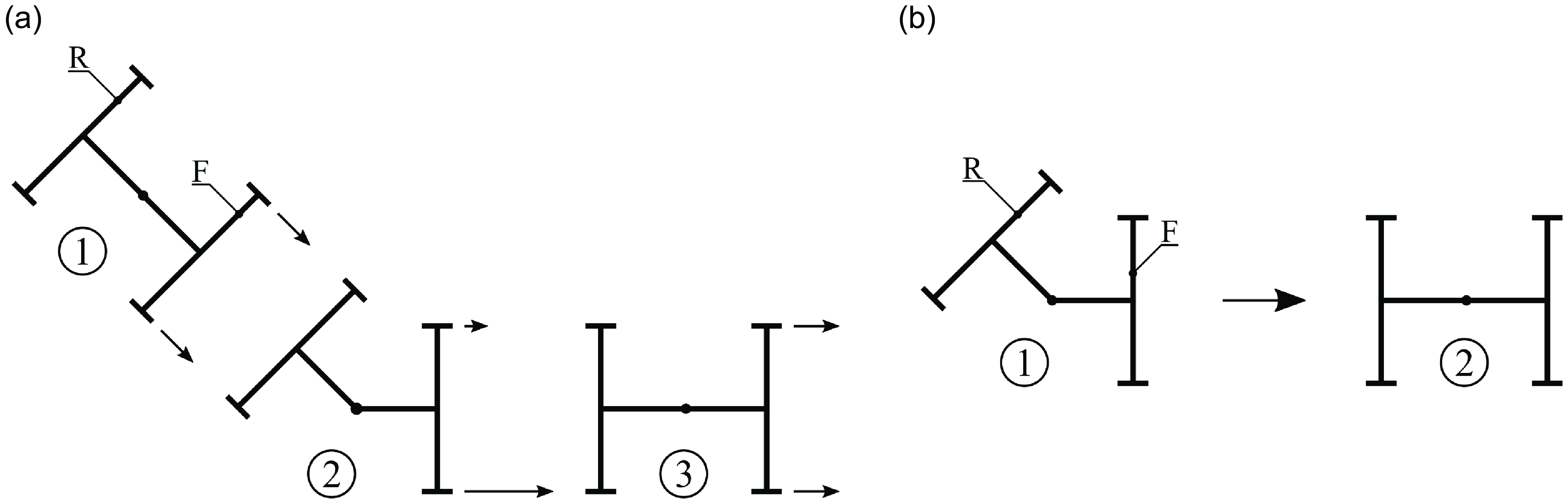
(a) Steering test scheme. (b) Standing start test scheme.

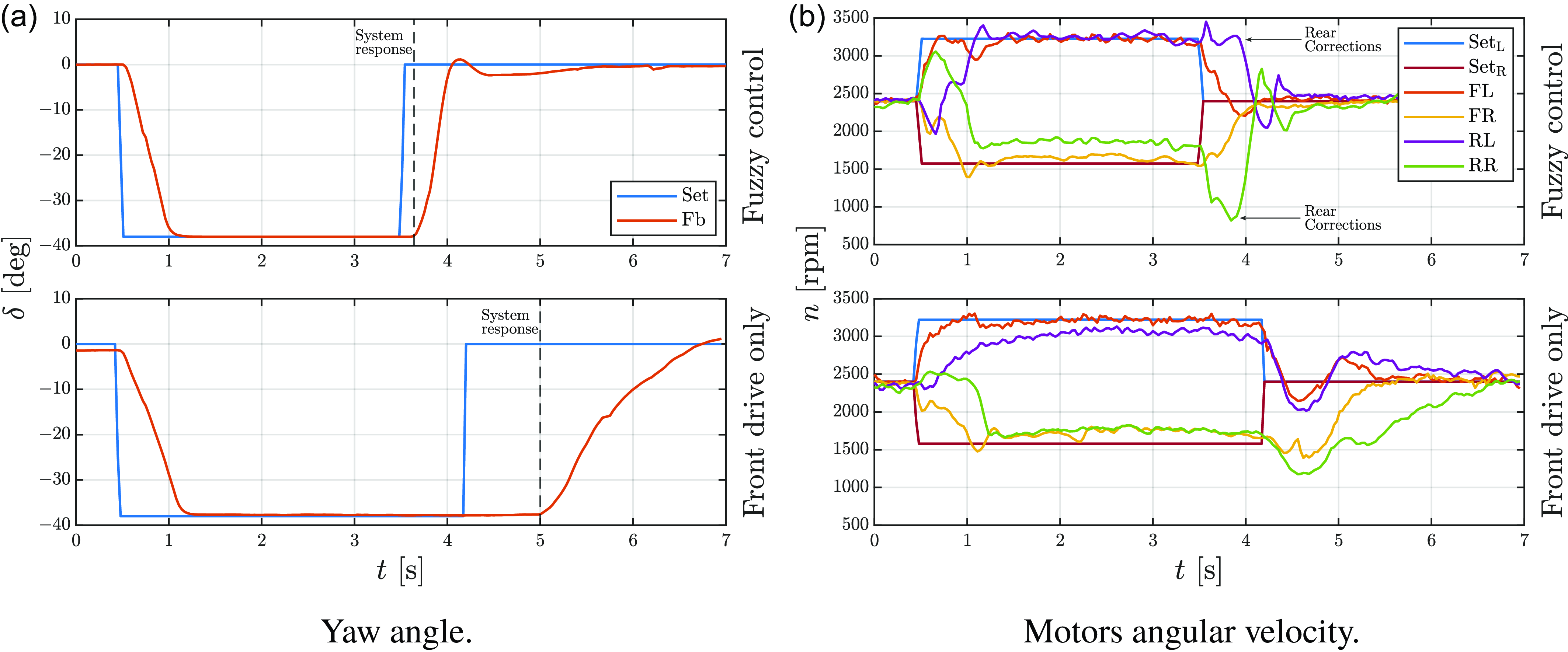
In the steering test (Figure 16a), the robot travels at a constant speed through a straight section (1), a curve (2), and a new straight section (3) to analyze its behavior while entering and, more importantly, exiting a curve. The test was performed in 8WD mode and 4WD mode to verify the different behaviors of the robot.
Figures 17a and 17b shows the yaw angle and the angular speed of the motors during the test, respectively. Looking first at the yaw angle graph, the main differences are in the transition between the curve and the straight section. In 8WD mode with fuzzy control enabled, Epi.Q takes about 0.5 s to reach the target angle. In contrast, in 4WD mode, there is a noticeable delay before the robot adjusts its steering, and then it takes about 2 s to reach the target angle. The time it takes Epi.Q to reach the target angle in 4WD mode results in a continuation of the curve, which makes the robot difficult to maneuver.
Looking at the angular speed graph, there is a clear difference in the robot’s behavior between 8WD and 4WD modes. In the first case, the rear module (RL, RR), with the high speed variation imposed by fuzzy control, helps to reorient the robot to quickly reach the target angle. In the second case, the rear module is just a trailer, so only the front module works to reach the final configuration.
Steering test. Fuzzy control actively works to reduce system time response.

4.4. Standing start test
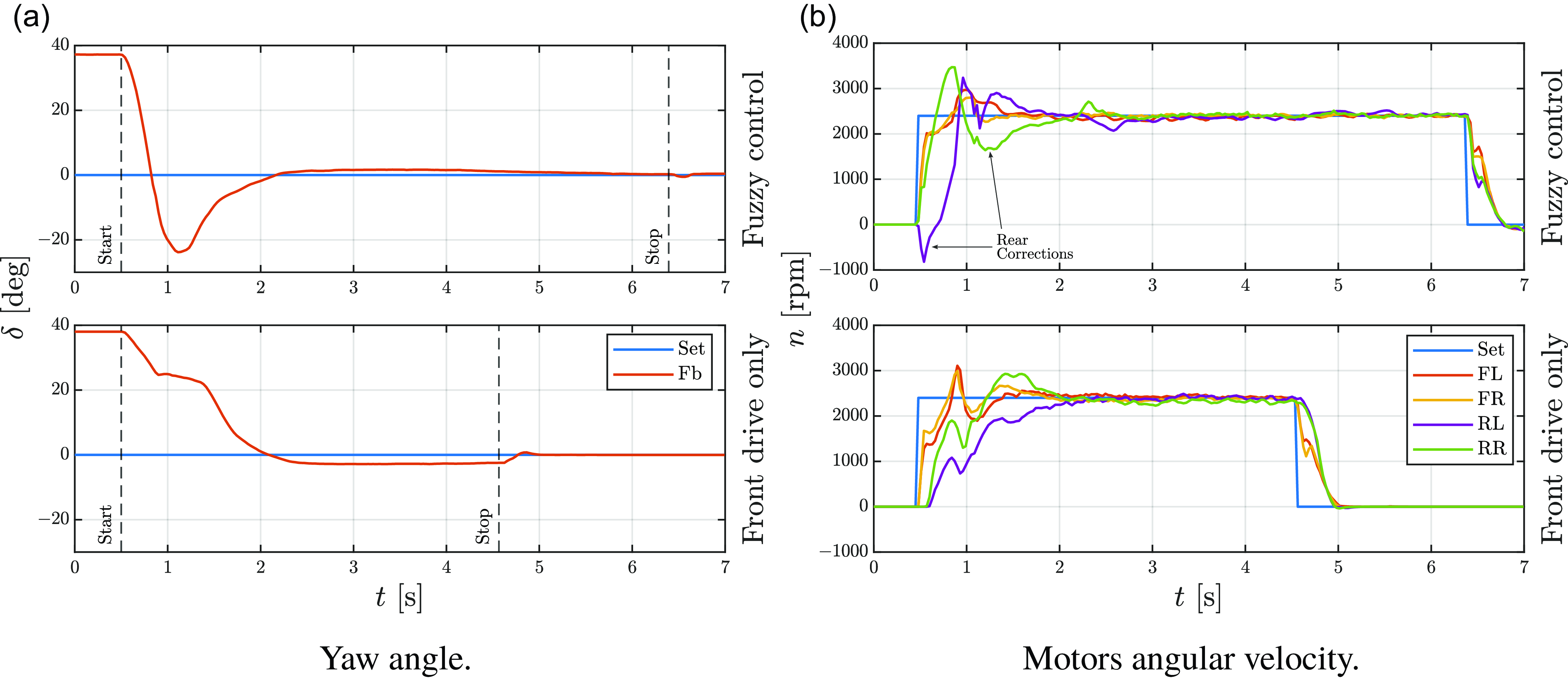
The standing start test (Figure 16b) consists of positioning the robot with the maximum misalignment between the modules, in this case
 $\delta = 38^\circ$
, and then applying a longitudinal velocity command to evaluate the acceleration phase and the realignment phase.
Standing start test. Fuzzy control changes the behavior of the system during the transient.

The yaw angle graph (Figure 18a) shows that although the time to reach the target angle is identical in both scenarios, the paths differ significantly, leading to different outcomes. In the first scenario (fuzzy control), the front module of Epi.Q essentially follows a straight path, meaning that the module does not rotate from its initial position. In the second case, however, the front module rotates from its initial position because of the resistance from the rear module during the acceleration phase. When the robot reaches module alignment, the front module does not go in the same direction as in the first case.
These observations can be deduced by examining Figure 18a and Figure 18b. The yaw angle sensor records an overshoot when fuzzy control is active, which is due to the correction made by the rear module. This substantial correction helps mitigate the drift phenomenon of the front module. Moreover, an important distinction is visible in the angular speed graph: the RL wheel reaches the target in 1 s with fuzzy control activated, whereas it takes approximately 2 s without it. This discrepancy allows the front module to maintain its initial direction.
4.5. Discussion of results
In conclusion, the preliminary tests performed on the Epi.Q UGV have highlighted its strengths and areas for potential improvement under various operational conditions.Footnote 2 The uphill tests showed that the fuzzy control and 8WD configuration significantly enhance Epi.Q’s climbing capabilities. The obstacle-climbing test further validated the effectiveness of the fuzzy control system, allowing Epi.Q to smoothly transition between flat and uneven surfaces, including steps, which would have been challenging in a 4WD configuration alone. The steering and standing start tests demonstrated the improved maneuverability and alignment control provided by the rear module’s fuzzy control, especially in maintaining trajectory and minimizing alignment delay after sharp turns or misalignments. Overall, these tests underscore the effectiveness of the fuzzy logic-based control in stabilizing the robot’s performance across diverse and unpredictable terrains, providing valuable insights for future optimization and refinement of the control system.
5. Conclusion
This paper presented the design, control strategy, and validation testing of the Epi.Q UGV, a modular robot developed for challenging environments. By implementing a fuzzy logic-based traction control system and a modular skid-steering system, the Epi.Q demonstrated notable stability and adaptability across various terrains, including steep inclines and uneven surfaces. Preliminary tests, such as hill climbing, obstacle navigation, and realignment under misalignment conditions, highlighted the effectiveness of the fuzzy control strategy in managing Epi.Q’s articulated 8WD configuration, enhancing traction and maneuverability. In addition, the robot’s tripod locomotion system and articulated structure allowed it to navigate complex surfaces.
It is important to note that a direct comparison with other methods such as MPC or SMC is not possible at this time because these methods require a dynamic model of the system, which is not currently available. The adoption of fuzzy logic control was a deliberate choice, as it allows bypassing the need for a precise dynamic model, providing a robust solution to handle the nonlinearities inherent in the system. This approach offers several advantages: it does not depend on a dynamic model, is simpler to implement, and requires significantly less computational power, making it ideal for real-time applications in dynamic and unstructured environments.
Although a fair comparison to MPC and SMC cannot be made at this time, the advantages of fuzzy logic control reinforce its suitability for addressing the challenges posed by Epi.Q’s operational context. These results validate Epi.Q’s ability to navigate effectively in unstructured environments and underscore the potential of fuzzy logic control to improve UGV performance. Future work will aim to optimize the fuzzy control system for greater efficiency and adaptability, including its performance in uneven terrain and highly dynamic environments. In addition, efforts will be directed toward integrating advanced sensor technologies to improve real-time decision making and extending the system’s capabilities to support modular scalability for more complex configurations.
Author contributions
Conceptualization, S.P., A.B., G.P. and G.Q.; methodology, S.P. and A.B.; software, S.P.; validation, S.P. and A.B.; formal analysis, S.P., A.B., G.P. and G.Q.; resources, G.P. and G.Q.; data curation, S.P.; writing – original draft preparation, S.P.; writing – review and editing, A.B., G.P and G.Q.; visualization, S.P. and A.B.; supervision, G.P. and G.Q.; project administration, G.P. and G.Q; funding acquisition, G.P. and G.Q. All authors have read and agreed to the published version of the manuscript.
Financial support
This research received no specific grant from any funding agency, commercial, or not-for-profit sectors.
Competing interests
The authors declare no conflicts of interest exist.
Ethical approval
Not applicable.