1 Introduction
Leaving aside the inherently mysterious peculiarities of turbulence, turbulent reacting flows are characterized by a complex interplay between hydrodynamic motions and heat released by the flame. Although sometimes useful for analytical purposes (Clavin Reference Clavin1985), an additional complexity of turbulent combustion arises from its multi-scale nature as these processes occur at very different time and length scales (Peters Reference Peters2009). With the progress of computing resources, numerical simulations, notably RANS (Reynolds-averaged Navier–Stokes) and LES (large eddy simulations), have become versatile tools for predicting the behaviour of turbulent flames in situations of industrial relevance. In the context of either RANS or LES, phenomenological models are required for assessing the unresolved phenomena and different strategies have been followed among which the geometrical description (which comprises both the level set and the flame surface density formalisms) is one of the most widely employed (Veynante & Vervisch Reference Veynante and Vervisch2002). In order to better understand the practical benefit and remaining issues of these approaches, we briefly describe the transport equations on which they rely.
Consider
 $Y_{f}$
the fuel mass fraction and
 $Y_{f}^{\ast }$
the reduced fuel mass fraction defined by
 $Y_{f}^{\ast }=(Y_{f}-Y_{f,b})/(Y_{f,u}-Y_{f,b})$
where
 $Y_{f,u}$
and
 $Y_{f,b}$
are the fuel mass fractions in the fresh and burned gases, respectively. The flame surface density description of turbulent flames provides a means to assess the volume-averaged (in a RANS or LES context) fuel reaction rate (Trouvé & Poinsot Reference Trouvé and Poinsot1994), viz.
 $$\begin{eqnarray}\displaystyle \overline{\dot{\unicode[STIX]{x1D714}}_{f}^{\ast }}=\unicode[STIX]{x1D70C}_{u}\langle S_{c}\rangle \unicode[STIX]{x1D6F4}. & & \displaystyle\end{eqnarray}$$
In (1.1),
 $\unicode[STIX]{x1D70C}_{u}$
is the density of the fresh mixture and
 $\dot{\unicode[STIX]{x1D714}}_{f}^{\ast }=\dot{\unicode[STIX]{x1D714}}_{f}/(Y_{f,u}-Y_{f,b})$
. The overbar denotes a volume average while the brackets represent a surface-weighted average which will be defined later. The flame consumption speed
 $S_{c}$
appearing in (1.1) is related to the fuel reaction rate through (Trouvé & Poinsot Reference Trouvé and Poinsot1994; Poinsot & Veynante Reference Poinsot and Veynante2005)
 $$\begin{eqnarray}\displaystyle S_{c}=-\frac{1}{\unicode[STIX]{x1D70C}_{u}}\int _{\unicode[STIX]{x1D702}=-\infty }^{\infty }{\dot{\unicode[STIX]{x1D714}}_{f}}^{\ast }\,\text{d}\unicode[STIX]{x1D702}, & & \displaystyle\end{eqnarray}$$
where
 $\unicode[STIX]{x1D702}$
is the direction normal to the flame. In (1.1),
 $\unicode[STIX]{x1D6F4}$
is the flame surface density whose transport equation writes (Candel & Poinsot Reference Candel and Poinsot1990; Trouvé & Poinsot Reference Trouvé and Poinsot1994)
 $$\begin{eqnarray}\displaystyle \frac{\unicode[STIX]{x2202}\unicode[STIX]{x1D6F4}}{\unicode[STIX]{x2202}t}+\unicode[STIX]{x1D735}\boldsymbol{\cdot }\langle \boldsymbol{w}\rangle \unicode[STIX]{x1D6F4}=\langle K\rangle \unicode[STIX]{x1D6F4}, & & \displaystyle\end{eqnarray}$$
where
 $\boldsymbol{w}=\boldsymbol{u}+S_{d}\boldsymbol{n}$
is the absolute speed of the flame in a fixed laboratory frame,
 $\boldsymbol{u}$
is the fluid velocity and
 $S_{d}$
is the displacement speed of the iso-surface considered, with
 $\boldsymbol{n}$
being the flame normal vector oriented towards the fresh gases. While
 $S_{c}$
is an integrated value along the flame normal direction,
 $\boldsymbol{u}$
,
 $\boldsymbol{w}$
and thus
 $S_{d}$
depend on the particular choice of the iso-surface used to track the flame. Equation (1.3) includes the total stretch rate
 $K$
which represents the relative increase in flame surface area. As shown by e.g. Matalon & Matkowsky (Reference Matalon and Matkowsky1982), Clavin & Joulin (Reference Clavin and Joulin1983), Candel & Poinsot (Reference Candel and Poinsot1990), the total stretch rate
 $K$
can be decomposed into two contributions, i.e.
 $K=K_{T}+K_{C}$
, one due to tangential strain rate
 $K_{T}=-\boldsymbol{n}\boldsymbol{n}\boldsymbol{ : }\unicode[STIX]{x1D735}\boldsymbol{u}+\unicode[STIX]{x1D735}\boldsymbol{\cdot }\boldsymbol{u}$
and the other one to the flame propagative/curved character
 $K_{C}=2S_{d}\unicode[STIX]{x1D705}_{m}$
. The curvature
 $\unicode[STIX]{x1D705}_{m}$
is defined as the average of the two principal curvatures
 $\unicode[STIX]{x1D705}_{1}$
and
 $\unicode[STIX]{x1D705}_{2}$
.
Equation (1.1) is particularly attracting because it decomposes the averaged fuel reaction rate into two contributions, one in the flame iso-surface reference frame (1.3), and another in the normal direction (1.2), thereby decoupling at least conceptually flame/turbulence interactions into geometrical aspects (i.e. the creation of flame surface through flame stretch) and kinematic aspects (i.e. the consumption rate of fuel).
Another approach for characterizing turbulent flames is the level-set approach which ignores the flame inner structure and considers explicitly only one particular flame iso-surface. This method is efficient in terms of computational cost as the phenomena occurring in flame normal direction do not need to be resolved on the computation mesh. In the context of either LES or RANS, Oberlack, Wenzel & Peters (Reference Oberlack, Wenzel and Peters2001), Pitsch (Reference Pitsch2005) obtained the following kinematic relation for the filtered flame iso-surface
 $$\begin{eqnarray}\displaystyle \frac{\unicode[STIX]{x2202}\check{G}}{\unicode[STIX]{x2202}t}+\langle \boldsymbol{u}\rangle \boldsymbol{\cdot }\unicode[STIX]{x1D735}\check{G}=\langle S_{d}\rangle A_{f}|\unicode[STIX]{x1D735}\check{G}|. & & \displaystyle\end{eqnarray}$$
Here
 $\check{G}$
is not the averaged
 $G$
-field but the level set of the filtered flame coordinates (Pitsch Reference Pitsch2005) and
 $A_{f}$
is the flame surface comprised in the averaging volume. Equation (1.4) also highlights the interaction between the flame geometrical properties, here the
 $G$
-field and the flame kinematic features through the appearance of the displacement speed.
In order to infer
 $S_{c}$
and
 $S_{d}$
, the flamelet hypothesis (Peters Reference Peters1986) is generally invoked. This assumption suggests that turbulent flames can be conceptualized as a collection of thin layers, whose inner structure is identical to a one-dimensional laminar flame, propagating normal to themselves in the direction of the unburned turbulent mixture. As a consequence, the notion of laminar flamelet implies that only the geometrical properties of the flame have to be explicitly characterized while the flame consumption or displacement speeds appearing in (1.1), (1.3) and (1.4) are inferred from simulations of one-dimensional (1-D) laminar flames prior to the turbulent reacting flow simulation. However, when curved and strained, the local inner flame structure generally does not remain identical to a laminar planar flame. Therefore, a more accurate modelling of the phenomena at play requires bridge building the knowledge of the internal structure of flames, gathered generally in laminar situations, to turbulent configurations. A very elegant example of such an achievement was recently provided by Fogla, Creta & Matalon (Reference Fogla, Creta and Matalon2015, Reference Fogla, Creta and Matalon2017).
It is well known that
 $S_{c}$
and
 $S_{d}$
can be locally affected by the flame geometrical properties. Karlovitz et al. (Reference Karlovitz, Denniston, Knapschaefer and Wells1953) were first to suggest that the flame propagation speed is proportional to the total stretch rate. This statement was later confirmed theoretically in the limit of single-step chemistry with large activation energy, i.e. in the context of the so-called Zeldovich Frank–Kamenetskii (ZFK) model (Clavin & Williams Reference Clavin and Williams1982; Matalon & Matkowsky Reference Matalon and Matkowsky1982). Later, the dependence of thermal conductivity to temperature have been taken into account (Clavin & Garcia Reference Clavin and Garcia1983; Bechtold & Matalon Reference Bechtold and Matalon2001). Theory indicates that the displacement and consumption speed should indeed vary linearly with respect to the total stretch rate, with coefficients of proportionality noted
 ${\mathcal{L}}_{d}$
and
 ${\mathcal{L}}_{c}$
, respectively, viz.
 $$\begin{eqnarray}\displaystyle S_{c,d}=S_{l}^{0}-K{\mathcal{L}}_{c,d}=S_{l}^{0}-(K_{T}+K_{C}){\mathcal{L}}_{c,d}, & & \displaystyle\end{eqnarray}$$
where
 $S_{l}^{0}$
is the flame propagation speed of an unstretched planar flame. Here
 ${\mathcal{L}}$
has the dimension of a length scale and is referred to as the Markstein length (Markstein Reference Markstein1964). The ratio of the Markstein length to the flame thickness
 $l_{f}$
is called the Markstein number
 ${\mathcal{M}}$
(Markstein Reference Markstein1964), where
 $l_{f}$
is defined by
 $D_{th}/S_{l}^{0}$
, with
 $D_{th}$
the thermal diffusivity. Functional expressions for
 ${\mathcal{L}}_{d}$
and
 ${\mathcal{L}}_{c}$
have been derived (Clavin & Garcia Reference Clavin and Garcia1983; Bechtold & Matalon Reference Bechtold and Matalon2001),
 $$\begin{eqnarray}\displaystyle {\mathcal{M}}_{c}=\frac{{\mathcal{L}}_{c}}{l_{f}} & = & \displaystyle \frac{1}{2}\frac{\unicode[STIX]{x1D6FD}(Le-1)}{\unicode[STIX]{x1D70E}-1}\int _{1}^{\unicode[STIX]{x1D70E}}\frac{\unicode[STIX]{x1D706}(\unicode[STIX]{x1D709})}{\unicode[STIX]{x1D709}}\text{ln}\left(\frac{\unicode[STIX]{x1D70E}-1}{\unicode[STIX]{x1D709}-1}\right)\,\text{d}\unicode[STIX]{x1D709}\end{eqnarray}$$
 $$\begin{eqnarray}\displaystyle {\mathcal{M}}_{d}^{u}=\frac{{\mathcal{L}}_{d}^{u}}{l_{f}} & = & \displaystyle \frac{{\mathcal{L}}_{c}}{l_{f}}+\frac{\unicode[STIX]{x1D70E}}{\unicode[STIX]{x1D70E}-1}\int _{1}^{\unicode[STIX]{x1D70E}}\frac{\unicode[STIX]{x1D706}(\unicode[STIX]{x1D709})}{\unicode[STIX]{x1D709}}\,\text{d}\unicode[STIX]{x1D709}.\end{eqnarray}$$
 $\unicode[STIX]{x1D6FD}$
is the reduced activation energy or Zeldovich number and
 $Le$
is the effective Lewis number as defined by e.g. Bechtold & Matalon (Reference Bechtold and Matalon2001). Equations (1.6a
) and (1.6b
) thus indicate that the sensitivity of flames to the stretch rate depends strongly on the Lewis number
 $Le$
. This effect should be more important in lean heavy hydrocarbon flames characterized by
 $Le>1$
than in stoichiometric methane/air flames for which the Lewis number is close to unity. The expansion rate
 $\unicode[STIX]{x1D70E}$
is defined as
 $\unicode[STIX]{x1D70E}=T_{b}/T_{u}$
, where
 $T_{u}$
and
 $T_{b}$
denote the temperature in the fresh and burned gases, respectively. Here
 $\unicode[STIX]{x1D706}$
is the thermal conductivity normalized by its value in the unburned gases and
 $\unicode[STIX]{x1D709}$
is an integration variable. Note that we give here the expression for
 ${\mathcal{L}}_{d}^{u}$
, i.e. the Markstein length relative to the unburned gases. An extension of
 ${\mathcal{L}}_{d}^{u}$
that accounts for arbitrary reaction orders is provided by Matalon, Cui & Bechtold (Reference Matalon, Cui and Bechtold2003).
Although meaningful for fundamental purposes, the use of these ‘laminar’ Markstein length-scales for predicting the evolution of
 $S_{d}$
and
 $S_{c}$
in turbulent reacting flows may not be appropriate for the following reasons.
-
(i) The total stretch rate may not be the only scalar quantity impacting flame kinematics. When asymptotic analysis was first conducted (Clavin & Williams Reference Clavin and Williams1982; Matalon & Matkowsky Reference Matalon and Matkowsky1982), it was not assumed a priori that curvature and strain rate affect the flame speed in a similar fashion. In other words, the appearance of an identical Markstein number for strain rate and curvature was not conjectured a priori but resulted from the asymptotic analysis, derived in the context of single step irreversible chemistry with large activation energy, reducing the flame zone to a surface of discontinuity. However, it is worth stressing that this result is only valid in this particular limit and may not be considered as a general result applicable to all situations. Indeed, when the mixture strength effect was included (Bechtold & Matalon Reference Bechtold and Matalon2001) or the dependence of flame speed to the reference surface in the flame made explicit (Bechtold & Matalon Reference Bechtold and Matalon2001; Giannakopoulos et al. Reference Giannakopoulos, Gatzoulis, Frouzakis, Matalon and Tomboulides2015a ), it was found that the dependence of flame speed to strain rate and curvature was different, leading to two distinct Markstein lengths, one characterizing the dependence of
 $S_{d}$
to stretch, the other to curvature. When the one-step chemistry assumption was replaced by multiple reactions (Clavin & Graña-Otero Reference Clavin and Graña-Otero2011), it turned out that the coefficients modulating the flame speed with respect to stretch and curvature were not similar. Similar results were obtained when heat losses were taken into account (Matalon & Bechtold Reference Matalon and Bechtold2009). Therefore, asymptotic analysis reveals that the dependence of flame speeds to strain rate and curvature might be different depending on the situation, and thus stretch is not the only scalar quantity affecting the flame speed. There is also numerical evidence (Haworth & Poinsot Reference Haworth and Poinsot1992; Rutland & Trouvé Reference Rutland and Trouvé1993) that turbulent premixed flames are more correlated to curvature than strain. Echekki & Chen (Reference Echekki and Chen1996) showed that highly diffusive species such as H and
$\text{H}_{2}$
are more influenced by curvature than the strain rate when compared to less diffusive species, such as CO. This reinforces the need of decoupling the effects of strain rate and curvature into two distinct contributions. However, it seems from the literature that (1.5) is taken as granted. Researchers remain focused only on the flame speed/stretch rate relationship although more recent theoretical studies have clearly indicated the important role played by curvature. The lack of recognition of the results provided by Bechtold & Matalon (Reference Bechtold and Matalon2001), Clavin & Graña-Otero (Reference Clavin and Graña-Otero2011), Giannakopoulos et al. (Reference Giannakopoulos, Gatzoulis, Frouzakis, Matalon and Tomboulides2015a
) is likely to be explained, to a large extent, by the lack of experimental or numerical validation.
To further substantiate the results from asymptotic theory showing a distinct dependence of flame speed to stretch rate and curvature, we recall the main result of Bechtold & Matalon (Reference Bechtold and Matalon2001), Giannakopoulos et al. (Reference Giannakopoulos, Gatzoulis, Frouzakis, Matalon and Tomboulides2015a ). These studies have shown that the displacement speed at a given isotherm writes (Bechtold & Matalon Reference Bechtold and Matalon2001; Giannakopoulos et al. Reference Giannakopoulos, Gatzoulis, Frouzakis, Matalon and Tomboulides2015a )
(1.7)where
$$\begin{eqnarray}\displaystyle \widetilde{S_{d}}(\unicode[STIX]{x1D703})=S_{l}^{0}-{\mathcal{L}}_{K}(\unicode[STIX]{x1D703})K-{\mathcal{L}}_{\unicode[STIX]{x1D705}}(\unicode[STIX]{x1D703})2S_{l}^{0}\unicode[STIX]{x1D705}_{m}, & & \displaystyle\end{eqnarray}$$
$\widetilde{S_{d}}$
is the density-weighted displacement speed, i.e.
$\widetilde{S_{d}}=\unicode[STIX]{x1D70C}S_{d}/\unicode[STIX]{x1D70C}_{u}$
at a given isotherm
$\unicode[STIX]{x1D703}=T/T_{u}$
. (Note that (1.7) is written here similarly to Giannakopoulos et al. (Reference Giannakopoulos, Gatzoulis, Frouzakis, Matalon and Tomboulides2015a
,Reference Giannakopoulos, Matalon, Frouzakis and Tomboulides
b
), i.e. two contributions are identified, one due to the stretch rate and the other to curvature. However, it is possible to split the stretch rate into a strain rate and a curvature component leading to two distinct Markstein lengths, one based on
$K_{T}$
which is
${\mathcal{L}}_{K}$
and another one based on
$K_{C}$
which then writes
${\mathcal{L}}_{K}+{\mathcal{L}}_{\unicode[STIX]{x1D705}}$
(assuming
$K_{C}=2S_{l}^{0}\unicode[STIX]{x1D705}_{m}$
). The reason for keeping (1.7) in this form is that in general
$K_{C}=2S_{d}\unicode[STIX]{x1D705}_{m}\neq 2S_{l}^{0}\unicode[STIX]{x1D705}_{m}$
. Furthermore,
${\mathcal{L}}_{K}$
is Lewis number dependent whereas
${\mathcal{L}}_{\unicode[STIX]{x1D705}}$
is not (Bechtold & Matalon Reference Bechtold and Matalon2001; Giannakopoulos et al.
Reference Giannakopoulos, Gatzoulis, Frouzakis, Matalon and Tomboulides2015a
,Reference Giannakopoulos, Matalon, Frouzakis and Tomboulides
b
). This will be more convenient, when discussing Lewis number effects.) In the ZFK framework, Bechtold & Matalon (Reference Bechtold and Matalon2001), Giannakopoulos et al. (Reference Giannakopoulos, Gatzoulis, Frouzakis, Matalon and Tomboulides2015a
,Reference Giannakopoulos, Matalon, Frouzakis and Tomboulides
b
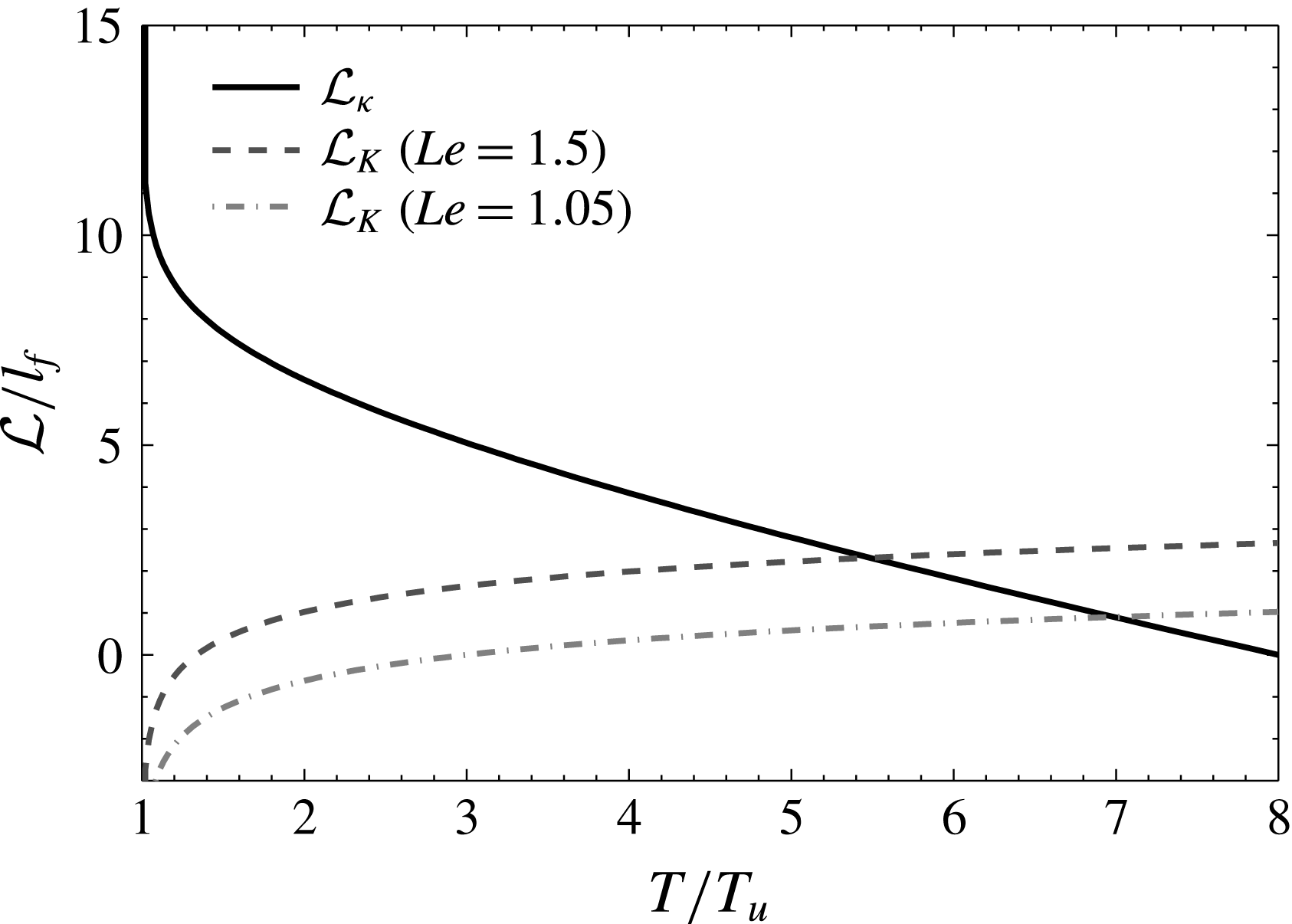
) provided the following functional expressions for the stretch rate and curvature Markstein lengths appearing in (1.7)Equation (1.7) emanates when considering explicitly the inner structure of the flame and particularly that of the preheat zone. This was anticipated by Clavin & Joulin (Reference Clavin and Joulin1989) who noticed that (1.5) is not generic since it is not invariant by surface change within the flame thickness. The finite thickness of the flame implies that the curvature and stretch Markstein numbers depend on the choice of iso-scalar within the flame and(1.8a )
$$\begin{eqnarray}\displaystyle & \displaystyle \frac{{\mathcal{L}}_{K}(\unicode[STIX]{x1D703})}{l_{f}}=\frac{{\mathcal{L}}_{d,u}}{l_{f}}-\int _{1}^{\unicode[STIX]{x1D703}}\frac{\unicode[STIX]{x1D706}(\unicode[STIX]{x1D709})}{\unicode[STIX]{x1D709}}\,\text{d}\unicode[STIX]{x1D709}-\int _{\unicode[STIX]{x1D703}}^{\unicode[STIX]{x1D70E}}\frac{\unicode[STIX]{x1D706}(\unicode[STIX]{x1D709})}{\unicode[STIX]{x1D709}-1}\,\text{d}\unicode[STIX]{x1D709} & \displaystyle\end{eqnarray}$$
(1.8b )
$$\begin{eqnarray}\displaystyle & \displaystyle \frac{{\mathcal{L}}_{\unicode[STIX]{x1D705}}(\unicode[STIX]{x1D703})}{l_{f}}=\int _{\unicode[STIX]{x1D703}}^{\unicode[STIX]{x1D70E}}\frac{\unicode[STIX]{x1D706}(\unicode[STIX]{x1D709})}{\unicode[STIX]{x1D709}-1}\,\text{d}\unicode[STIX]{x1D709}. & \displaystyle\end{eqnarray}$$
${\mathcal{L}}_{K}$
changes sign from the fresh to burned gases (Giannakopoulos et al.
Reference Giannakopoulos, Gatzoulis, Frouzakis, Matalon and Tomboulides2015a
,Reference Giannakopoulos, Matalon, Frouzakis and Tomboulides
b
). Equation (1.7) together with (1.8) have been validated by Giannakopoulos et al. (Reference Giannakopoulos, Gatzoulis, Frouzakis, Matalon and Tomboulides2015a
,Reference Giannakopoulos, Matalon, Frouzakis and Tomboulides
b
) from numerical simulation of steady spherical flames. However, the experimental configurations in which this (these) Markstein length(s) is (are) assessed do not allow the effect of stretch and curvature to be distinguished. Indeed, among the methods used to infer Markstein lengths, the spherically expanding flame in a closed vessel is one of the most common (see e.g. Halter, Tahtouh & Mounaïm-Rousselle (Reference Halter, Tahtouh and Mounaïm-Rousselle2010), Balusamy, Cessou & Lecordier (Reference Balusamy, Cessou and Lecordier2011), Varea (Reference Varea2013) and references therein). In this case, both strain rate and curvature have the same sign and are proportional to each other, thus precluding any distinction between strain rate and curvature. Another configuration is the counterflow flame (Vagelopoulos, Egolfopoulos & Law Reference Vagelopoulos, Egolfopoulos and Law1994; Chao, Egolfopoulos & Law Reference Chao, Egolfopoulos and Law1997; Egolfopoulos, Zhang & Zhang Reference Egolfopoulos, Zhang and Zhang1997; Vagelopoulos & Egolfopoulos Reference Vagelopoulos and Egolfopoulos1998; Bouvet Reference Bouvet2009) which is strained but has zero curvature. There is thus a need for configurations in which the effect of stretch and curvature can be distinguished. The above comments on the effect of stretch rate and curvature were devoted to the flame displacement speed, while it remains unclear whether the same distinction applies to the consumption speed. Asymptotic theory (Bechtold & Matalon Reference Bechtold and Matalon2001) indicates that
$S_{c}$
is only affected by stretch while direct numerical simulations (DNSs) of turbulent premixed flames (Haworth & Poinsot Reference Haworth and Poinsot1992; Rutland & Trouvé Reference Rutland and Trouvé1993; Chen & Im Reference Chen and Im2000; Bell et al.
Reference Bell, Cheng, Day and Shepherd2007, for example) indicate that scatter plots of
$S_{c}$
versus
$K$
do not fall on a line and that curvature has a strong (if not dominant) additional effect.
-
(ii) Nonlinear effects are likely to dominate. There is no doubt that experiments and direct numerical simulations have been useful to confirm the validity of asymptotic theories and notably the adequacy of the functional expressions for the Markstein lengths. However, they also have highlighted the limits of the linear dependence of flame speeds to the stretch rate (Chen & Ju Reference Chen and Ju2007; Chen, Burke & Ju Reference Chen, Burke and Ju2009; Halter et al. Reference Halter, Tahtouh and Mounaïm-Rousselle2010). Since in turbulent flames, magnitudes of the strain rate and curvature are expected to be rather large, one may expect nonlinear effects to be predominant. This thus a priori precludes the use of (1.5) for assessing
$S_{c}$
and
$S_{d}$
in level-set or flame-surface density approaches. -
(iii) Transients are most likely important. In counter-flow or wall-stabilized burners, the flame is stationary whereas transient effects might be crucial in turbulent flames. For instance Mueller et al. (Reference Mueller, Driscoll, Reuss and Drake1996) have experimentally shown that, for a time lag comparable with the chemical time scale, laminar flames are weakly affected by external stretch rates, even if the rates are 10 times greater than the steady extinction stretch rate. Samaniego & Mantel (Reference Samaniego and Mantel1999) and Mantel & Samaniego (Reference Mantel and Samaniego1999) did not indicate any flame quenching in flame/vortex interaction at strain rates much higher than the steady extinction stretch rate. Im & Chen (Reference Im and Chen2000) have also shown that the flame speed/flame stretch correlation is strongly affected by the flow forcing frequency and can even vanish at high forcing frequencies in agreement with the theoretical predictions of Joulin (Reference Joulin1994), Clavin & Joulin (Reference Clavin and Joulin1997). Transient effects are also important for characterizing the flame geometrical properties, for instance flame stretch (Thiesset et al. Reference Thiesset, Maurice, Halter, Mazellier, Chauveau and Gökalp2017).
-
(iv) These effects might be smoothed when applying surface averaging. Irrespectively of the method used (level-set or flame surface density), the flame geometrical (stretch rate, curvature) and kinematic properties (flow velocity, flame displacement or consumption speed) altogether appear in brackets in the transport equations presented previously. This means that area-weighted (within the sub-grid scales) values are needed, not the local values (as the function of position on the flame). In this context, one could expect the averaging operation to smooth out the fluctuations of both
$S_{c}$
and
$S_{d}$
and blur their dependence to
$K,K_{C},K_{T}$
. For example, one may speculate that, within a given control volume, a flame is equally convex and concave leading to an area-weighted value of curvature close to zero, i.e.
$\langle K_{C}\rangle \approx 0$
, as observed in turbulent flames (Haworth & Poinsot Reference Haworth and Poinsot1992). In this situation, the influence of curvature on flame speeds should on average vanish.





In the present paper, the aim is to push the analysis one step forward by providing a detailed analysis of the kinematic and geometric response of flames of different Lewis numbers in an intermediate experimental configuration between laminar stretched flames (spherical or wall stabilized) and turbulent flames: a flame interacting with a vortex (abbreviated by FVI). Focus is shed particularly on item (i), i.e. the dependence of the flame kinematic properties (flame displacement and consumption speed) to the total stretch rate, curvature and the strain rate in a situation where the flame is not subject to thermo-diffusive nor hydrodynamic instabilities. The main target is to address whether or not the effect of stretch and curvature on the flame speeds (both the displacement and consumption speed) is the same.
There is a wealth of experimental (Roberts & Driscoll Reference Roberts and Driscoll1991; Roberts et al. Reference Roberts, Driscoll, Drake and Goss1993; Mueller et al. Reference Mueller, Driscoll, Reuss and Drake1996; Samaniego & Mantel Reference Samaniego and Mantel1999; Sinibaldi et al. Reference Sinibaldi, Driscoll, Mueller, Donbar and Carter2003; Thiesset et al. Reference Thiesset, Maurice, Halter, Mazellier, Chauveau and Gökalp2017) and numerical (Poinsot, Veynante & Candel Reference Poinsot, Veynante and Candel1991; Mantel & Samaniego Reference Mantel and Samaniego1999; Colin et al. Reference Colin, Ducros, Veynante and Poinsot2000; Charlette, Meneveau & Veynante Reference Charlette, Meneveau and Veynante2002; Bougrine et al. Reference Bougrine, Richard, Colin and Veynante2014) studies devoted to FVIs. A review by Renard et al. (Reference Renard, Thevenin, Rolon and Candel2000) was also dedicated to this topic. As discussed by Steinberg & Driscoll (Reference Steinberg and Driscoll2010), FVI remains rather far from the phenomena at play in real turbulent flames (no vortex stretching nor sweeping nor tilting, very long lifetime of the vortex, etc.). However, this situation is often employed as a benchmark for many fundamental purposes. Investigations on FVIs have notably led to the construction of the so-called spectral diagrams (Poinsot et al. Reference Poinsot, Veynante and Candel1991; Roberts et al. Reference Roberts, Driscoll, Drake and Goss1993) which allow us to identify the conditions needed for a vortex to stretch the flame, to create pockets of fresh gases or to locally quench the flame. In addition, these results yielded expression of efficiency functions, i.e. the transfer function between vortex strength and flame stretch (Colin et al. Reference Colin, Ducros, Veynante and Poinsot2000; Charlette et al. Reference Charlette, Meneveau and Veynante2002; Bougrine et al. Reference Bougrine, Richard, Colin and Veynante2014; Thiesset et al. Reference Thiesset, Maurice, Halter, Mazellier, Chauveau and Gökalp2017) which are largely employed in LES of turbulent premixed combustion. It is also an archetypal situation in which some experimentally measurable surrogates of the heat release can be tested (Najm et al. Reference Najm, Paul, Mueller and Wyckoff1998).
The present study focuses on the FVI configuration so that phenomena (i) to (iv) are likely to be perceived. Indeed, a vortex is first a time-dependent perturbation which allows us to investigate transient effects (see item (iii)) as shown by Mueller et al. (Reference Mueller, Driscoll, Reuss and Drake1996), Mantel & Samaniego (Reference Mantel and Samaniego1999), Samaniego & Mantel (Reference Samaniego and Mantel1999). Second both strain rate and curvature are present. There is also a chance of being able to control to some extent the relative contribution of strain rate and curvature to the total stretch rate. It is thus the ideal configuration for investigating the relative impact of
 $K_{T}$
and
 $K_{C}$
on
 $S_{c}$
and
 $S_{d}$
(see item (i)). Third, we can generate intense vortices compared to the flame characteristics since we can control both flow and flame parameters. The transition from a linear to a nonlinear effect of
 $K$
on
 $S_{c}$
and
 $S_{d}$
can thus possibly be assessed (see item (ii)). Here, we focus on some weak vortices so that nonlinear effects are not likely to be perceived. This issue is left for future investigations. Last but not least, FVI is convenient both experimentally and analytically as we can take advantage of the symmetry of the configuration (in our case, symmetry of revolution).
The paper is organized as follows. First, the experimental and numerical tools used for the present investigation are portrayed in § 2. Then the derivation of a measurable expression for the flame consumption speed is presented in § 3 and validated against experimental and numerical data in § 4. The flame geometric and kinematic features are then studied as a function of the vortex strength and Lewis number in § 5. In the latter section the distinct effect of stretch rate and curvature on the flame speeds is highlighted.
2 Tools of investigation
2.1 The flame–vortex interaction burner (FVIB)
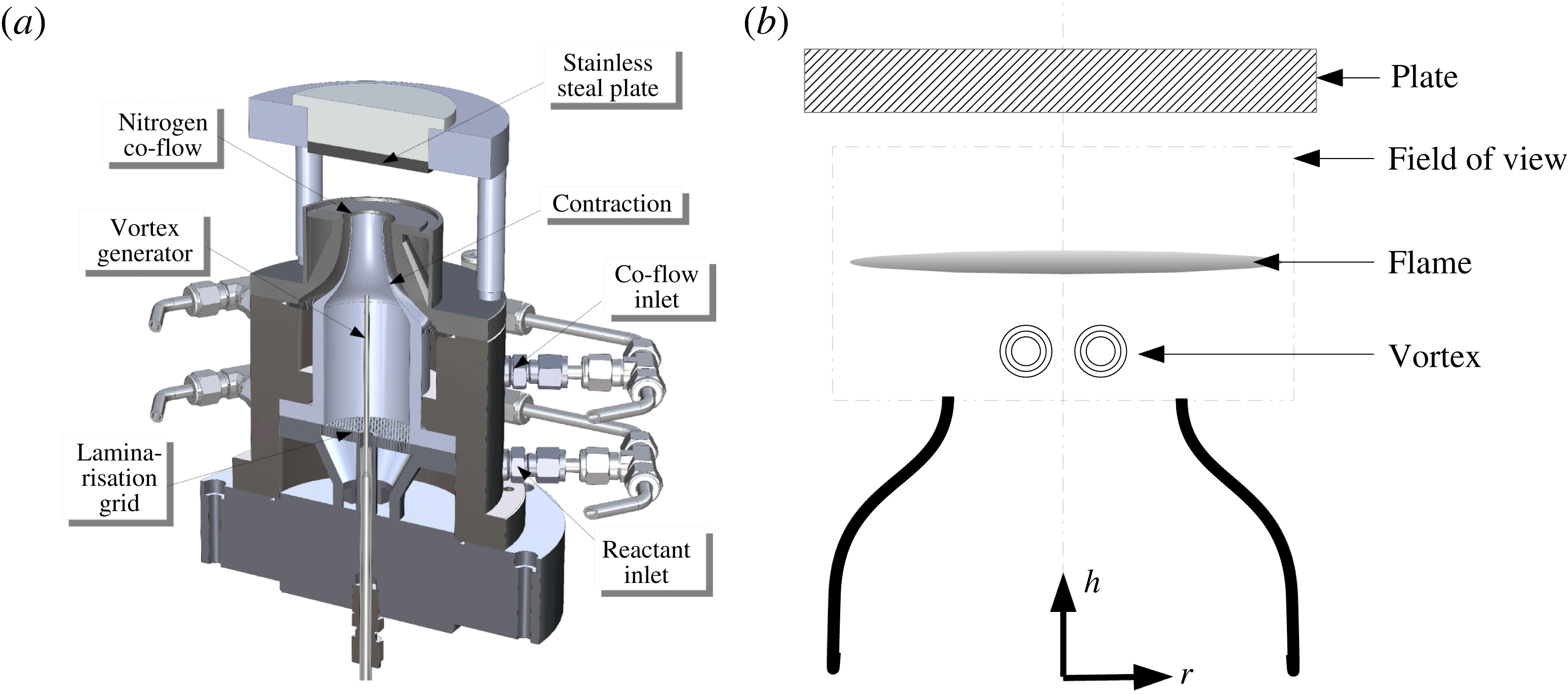
Experiments are carried out at ICARE, Orléans, in the burner used by Thiesset et al. (Reference Thiesset, Maurice, Halter, Mazellier, Chauveau and Gökalp2017) and presented in figure 1. Fuel and oxidizer are mixed before being fed through the side of the burner. The reactive mixture then flows into the burner plenum through a 5 mm thick aluminium grid whose role is to prevent turbulent structures being convected in the burner. A contraction ending with a 15 mm diameter is used to create a nearly top hat velocity profile with low turbulent intensity at the burner exit. The burner-to-stagnation plate distance is 25 mm and the outlet velocity is such that the flame is stabilized approximately 10 mm downstream the burner outlet, i.e. 15 mm upstream the stagnation plate. During the interaction with the vortex, the minimum distance between the flame and the wall is approximately 8 mm. This allows us to investigate FVIs without being affected by any wall effects. This large burner-to-stagnation plate distance also minimizes the tangential strain rate at steady state before interaction with the vortex. To avoid external perturbations and improve flame stability, a laminar coaxial shroud of nitrogen is used. The exit co-flow velocity is
 $0.1~\text{m}~\text{s}^{-1}$
.
Schematic of the flame–vortex interaction burner (FVIB).

Here, we consider propane/air and methane/air mixtures to investigate the sensitivity of the total stretch rate, flame curvature, together with the consumption and displacement speed to the Lewis number effects. Indeed, a stoichiometric methane/air mixture is characterized by an effective Lewis number close to unity whilst the Lewis number of a lean (e.g.
 $\unicode[STIX]{x1D719}=0.9$
) propane/air mixture is approximately 1.5.
The toroidal vortex generator consists of a tube of 2 mm in diameter located on the centreline, 35 mm upstream the burner outlet (figure 1). This tube is connected to a pressurized tank located upstream. The vortex is generated by applying a sudden pressure discharge of reactive mixture at the same equivalence ratio as the main flow. The intensity of the vortex is controlled by varying the pressure magnitude within the pressurized tank. To control the duration of the pressure discharge, we use two electro-valves (Thiesset et al. Reference Thiesset, Maurice, Halter, Mazellier, Chauveau and Gökalp2017).
Flame front positions and velocity fields are simultaneously measured by means of Mie scattering laser tomography (Boyer Reference Boyer1980). The flow is seeded with di-ethyl-hexyl-sebacate (DEHS) droplets supplied by an atomizer. Typical size of the droplets is approximately
 $1~\unicode[STIX]{x03BC}\text{m}$
. The light source is a continuous Coherent Verdi G20 Laser which can deliver up to 20 W at 532 nm. A laser power of 2.5 W was sufficient in the present case. The light scattered by the droplets is captured by a Phantom V1611 camera, equipped with a Sigma EX 180 mm 1:2.8 Macro, working at an acquisition rate of 21 000 Hz with a field of view of
 $896\times 800~\text{pixels}^{2}$
. The camera magnification is
 $36.72~\text{px}~\text{mm}^{-1}$
while the laser sheet thickness is approximately 0.5 mm.
The spatial location of the flame is close to the position at which the DEHS droplets evaporate. In the present case, the evaporation temperature of the droplets is 525 K. The flame contour is extracted using a classic threshold technique. More precisely, the Otsu (Reference Otsu1979) method (implemented in MATLAB) is used. This yields estimations for the progress variable, noted
 $\unicode[STIX]{x1D713}$
, which is by definition 0 and 1 in the unburned and burned gases, respectively. However, it is worth stressing that the isotherm which is tracked may not be exactly 525 K as the threshold employed in the binarization procedure which is based on the grey scale histogram is not likely to correspond exactly to this iso-temperature.
The Cartesian coordinates are denoted
 $x,y,z$
for characterizing the streamwise, transverse and spanwise direction, respectively. The cylindrical coordinates system are denoted
 $r,h,\unicode[STIX]{x1D703}$
for the radial, longitudinal and angular directions, respectively. Note that because of the axisymmetric geometry of the FVIB, we have
 $\unicode[STIX]{x2202}\bullet /\unicode[STIX]{x2202}\unicode[STIX]{x1D703}=0$
. A list of useful features of the surfaces of revolution is given in appendix A. Note that thanks to axisymmetry, we can access the two principal curvature components of the flame
 $\unicode[STIX]{x1D705}_{1}$
and
 $\unicode[STIX]{x1D705}_{2}$
and thus evaluate the 3-D curvature.
The velocity field within the unburned mixture is estimated by classical planar particle image velocimetry (PIV). For this purpose, the MATLAB subroutines of Thielicke & Stamhuis (Reference Thielicke and Stamhuis2014) were used. PIV processing was performed with a cross-correlation technique between pairs of successive images. The initial size of the PIV interrogation window was
 $32~\text{pix}^{2}$
. Four iterations were used to obtain a final interrogation window size of
 $16~\text{pix}^{2}$
, with a 50 % overlap. The vortex parameters, i.e. the circumferential velocity
 $U_{\unicode[STIX]{x1D703}}$
, the convection velocity
 $U_{c}$
and the core-to-core distance
 $R_{v}$
, have been inferred from PIV following the same procedure as Thiesset et al. (Reference Thiesset, Maurice, Halter, Mazellier, Chauveau and Gökalp2017). As said before, we use weak vortices with the aim of leaving aside nonlinear effects of stretch rate on the flame speeds. The experimental database covers the range
 $0.5\lesssim U_{\unicode[STIX]{x1D703}}/S_{L}\lesssim 3$
whereas
 $R_{v}/\unicode[STIX]{x1D6FF}_{th}$
slightly varies around 7.
 $\unicode[STIX]{x1D6FF}_{th}$
is the thermal flame thickness based on the maximum temperature gradient. The experimental operating conditions lie between the no-effect limit and the quenching limit assessed by Poinsot et al. (Reference Poinsot, Veynante and Candel1991), Roberts et al. (Reference Roberts, Driscoll, Drake and Goss1993). Note that, due to the strain rate in the tangential direction,
 $R_{v}$
increases when the vortex travels from the burner exit to the flame (Thiesset et al.
Reference Thiesset, Maurice, Halter, Mazellier, Chauveau and Gökalp2017). The values of
 $R_{v}$
and
 $U_{\unicode[STIX]{x1D703}}$
which are given here correspond to the values just before the vortex starts interacting with the flame.
2.2 Numerical simulations of FVIs
Direct numerical simulations of flame/vortex interactions have now become very common (Poinsot et al. Reference Poinsot, Veynante and Candel1991; Najm et al. Reference Najm, Paul, Mueller and Wyckoff1998; Mantel & Samaniego Reference Mantel and Samaniego1999; Colin et al. Reference Colin, Ducros, Veynante and Poinsot2000; Charlette et al. Reference Charlette, Meneveau and Veynante2002; Bougrine et al. Reference Bougrine, Richard, Colin and Veynante2014). Here, similar simulations are carried out using the high-order code AVBP (Schønfeld & Rudgyard Reference Schønfeld and Rudgyard1999; Moureau et al. Reference Moureau, Lartigue, Sommerer, Angelberger, Colin and Poinsot2005) developed by CERFACS and IFP-EN. AVBP solves the 3-D compressible Navier–Stokes equations using either a DNS or a LES strategy, on unstructured and hybrid meshes, using a cell vertex (CV) approach. The third order in time and space two-step Taylor–Galerkin finite element scheme TTGC (Colin & Rudgyard Reference Colin and Rudgyard2000) was used for its accuracy on the propagation of vortices. The boundary conditions were implemented with the Navier–Stokes characteristic boundary conditions (Poinsot & Lele Reference Poinsot and Lele1992). As done by Poinsot et al. (Reference Poinsot, Veynante and Candel1991), Bougrine et al. (Reference Bougrine, Richard, Colin and Veynante2014), only half of the domain was simulated by taking advantage of the symmetry. Combustion kinetics was described using the 19 species scheme of Lu & Law (Reference Lu and Law2008). For species diffusion, use is made of the mixture-averaged approach. The initial velocity field is prescribed using a Taylor-type (Gaussian) vortex (Wu, Ma & Zhou Reference Wu, Ma and Zhou2007), viz.
 $$\begin{eqnarray}\displaystyle U(R)=U_{\unicode[STIX]{x1D703}}\frac{R^{2}}{R_{c}^{2}}\exp \left(-\frac{R^{2}}{2R_{c}^{2}}\right), & & \displaystyle\end{eqnarray}$$
where
 $U_{\unicode[STIX]{x1D703}}$
is the characteristic vortex velocity,
 $R_{c}$
is the vortex core radius and
 $R=\sqrt{(x-x_{c})^{2}+(y-yc)^{2}}$
is the vortex radial coordinate.
 $x_{c}$
and
 $y_{c}$
denote the locations of the vortex centres. The vortex centre is initially positioned at
 $y_{c}/L_{y}=0.3,x_{c}/L_{x}=0.15$
before interacting with the flame which is initially located at
 $x/L_{x}=0.3$
(
 $L_{x}=0.0351$
m and
 $L_{y}=0.0167$
m are the sizes of the computational domain in the streamwise and spanwise directions, respectively). The ratio of the vortex maximum circumferential velocity
 $U_{\unicode[STIX]{x1D703}}$
to the laminar flame speed is set as 1. This value is similar to the experimental case analysed below. As in the experiment, the vortex core-to-core distance (
 $R_{v}=2y_{c}$
) is equal to
 $7\unicode[STIX]{x1D6FF}_{th}$
and the vortex core radius is
 $R_{c}=R_{v}/3$
. The grid size is
 $1340\times 638$
in the streamwise and spanwise directions, respectively.
3 Analytical considerations
One particular outcome of the present work is to provide a means to experimentally assess the flame kinematic properties, i.e. flame displacement and more importantly consumption speeds. While the displacement speed is measurable (see e.g. Sinibaldi, Mueller & Driscoll Reference Sinibaldi, Mueller and Driscoll1998; Renou et al.
Reference Renou, Boukhalfa, Puechberty and Trinité1998, Reference Renou, Boukhalfa, Puechberty and Trinité2000; Sinibaldi et al.
Reference Sinibaldi, Driscoll, Mueller, Donbar and Carter2003; Kerl, Lawn & Beyrau Reference Kerl, Lawn and Beyrau2013), the consumption speed is much more difficult to measure as the fuel reaction rate appearing in (1.2) is not experimentally accessible. Some studies (Najm et al.
Reference Najm, Paul, Mueller and Wyckoff1998) reveal that surrogates of the heat release such as
 $\text{CO}_{2}^{\ast }$
,
 $\text{CH}^{\ast }$
,
 $\text{OH}^{\ast }$
, HCO can be employed. However, these surrogates are unequally appropriate (Najm et al.
Reference Najm, Paul, Mueller and Wyckoff1998), and the relationship between fuel reaction rate and measured intensity of these surrogates may not hold in general. Here, we propose a novel approach inspired by previous work on spherical flames (Chung & Law Reference Chung and Law1988; Bradley, Gaskell & Gu Reference Bradley, Gaskell and Gu1996; Poinsot & Veynante Reference Poinsot and Veynante2011; Lefebvre et al.
Reference Lefebvre, Larabi, Moureau, Lartigue, Varea, Modica and Renou2016) or turbulent flames (Shepherd & Kostiuk Reference Shepherd and Kostiuk1994).
3.1 General expression for the flame consumption speed
A proper method to quantify
 $S_{c}$
is to start by integrating the fuel mass fraction equation over a given control volume (Chung & Law Reference Chung and Law1988; Bradley et al.
Reference Bradley, Gaskell and Gu1996; Poinsot & Veynante Reference Poinsot and Veynante2011; Lefebvre et al.
Reference Lefebvre, Larabi, Moureau, Lartigue, Varea, Modica and Renou2016). This method is generally referred to as the integral approach (Chung & Law Reference Chung and Law1988). The transport equation for the reduced fuel mass fraction
 $Y_{f}^{\ast }$
writes
 $$\begin{eqnarray}\displaystyle \frac{\unicode[STIX]{x2202}\unicode[STIX]{x1D70C}Y_{f}^{\ast }}{\unicode[STIX]{x2202}t}+\unicode[STIX]{x1D735}\boldsymbol{\cdot }(\boldsymbol{u}+\boldsymbol{v}_{f})\unicode[STIX]{x1D70C}Y_{f}^{\ast }=\dot{\unicode[STIX]{x1D714}}_{f}^{\ast }, & & \displaystyle\end{eqnarray}$$
where
 $\unicode[STIX]{x1D70C}$
is the density,
 $\boldsymbol{u}$
the local fluid velocity and
 $\boldsymbol{v}_{f}$
is the fuel diffusion velocity. The integration of (3.1) over an arbitrary material volume
 ${\mathcal{V}}(t)$
which comprises the flame writes
 $$\begin{eqnarray}\displaystyle \underbrace{\iiint _{{\mathcal{V}}(t)}\frac{\unicode[STIX]{x2202}\unicode[STIX]{x1D70C}Y_{f}^{\ast }}{\unicode[STIX]{x2202}t}\,\text{d}^{3}V}_{\text{NS}}+\underbrace{\iiint _{{\mathcal{V}}(t)}[\unicode[STIX]{x1D735}\boldsymbol{\cdot }(\boldsymbol{u}+\boldsymbol{v}_{f})\unicode[STIX]{x1D70C}Y_{f}^{\ast }]\,\text{d}^{3}V}_{\text{CD}}=\underbrace{\iiint _{{\mathcal{V}}(t)}\dot{\unicode[STIX]{x1D714}}_{f}^{\ast }\,\text{d}^{3}V}_{\text{RR}}. & & \displaystyle\end{eqnarray}$$
First, for the time derivative term (NS), by virtue of the Leibniz–Reynolds transport theorem we have
 $$\begin{eqnarray}\displaystyle \text{NS}=\iiint _{{\mathcal{V}}(t)}\frac{\unicode[STIX]{x2202}\unicode[STIX]{x1D70C}Y_{f}^{\ast }}{\unicode[STIX]{x2202}t}\,\text{d}^{3}V=\frac{\text{d}}{\text{d}t}\iiint _{{\mathcal{V}}(t)}\unicode[STIX]{x1D70C}Y_{f}^{\ast }\,\text{d}^{3}V-\unicode[STIX]{x0222F}_{\unicode[STIX]{x2202}{\mathcal{V}}(t)}\unicode[STIX]{x1D70C}Y_{f}^{\ast }(\boldsymbol{w}\boldsymbol{\cdot }\boldsymbol{n})\,\text{d}^{2}A, & & \displaystyle\end{eqnarray}$$
where
 $\boldsymbol{w}$
is the local (absolute) displacement speed of the volume boundary
 $\unicode[STIX]{x2202}{\mathcal{V}}(t)$
and
 $\boldsymbol{n}$
is the outward-pointing unit normal to
 $\unicode[STIX]{x2202}{\mathcal{V}}(t)$
. By use of the Green–Ostogradsky theorem, the convection–diffusion term CD simplifies to
 $$\begin{eqnarray}\displaystyle \text{CD}=\iiint _{{\mathcal{V}}(t)}[\unicode[STIX]{x1D735}\boldsymbol{\cdot }(\boldsymbol{u}+\boldsymbol{v}_{f})\unicode[STIX]{x1D70C}Y_{f}^{\ast }]\,\text{d}^{3}V=\unicode[STIX]{x0222F}_{\unicode[STIX]{x2202}{\mathcal{V}}(t)}[\unicode[STIX]{x1D70C}Y_{f}^{\ast }(\boldsymbol{u}+\boldsymbol{v}_{f})\boldsymbol{\cdot }\boldsymbol{n}]\,\text{d}^{2}A. & & \displaystyle\end{eqnarray}$$
The reaction rate term (RR) is expressed using the flame curvilinear coordinates defined by the normal, tangent and binormal (not necessarily unit) vectors, noted
 $\boldsymbol{\unicode[STIX]{x1D702}}$
,
 $\unicode[STIX]{x1D749}$
and
 $\unicode[STIX]{x1D737}$
, i.e. the flame Darboux frame. The volume element then writes
 $$\begin{eqnarray}\displaystyle \text{d}^{3}V=\text{d}x\,\text{d}y\,\text{d}z=\left|\frac{\unicode[STIX]{x2202}(x,y,z)}{\unicode[STIX]{x2202}(\unicode[STIX]{x1D702},\unicode[STIX]{x1D70F},\unicode[STIX]{x1D6FD})}\right|\text{d}\unicode[STIX]{x1D702}\,\text{d}\unicode[STIX]{x1D70F}\,\text{d}\unicode[STIX]{x1D6FD}=|\boldsymbol{J}|\,\text{d}\unicode[STIX]{x1D702}\,\text{d}\unicode[STIX]{x1D70F}\,\text{d}\unicode[STIX]{x1D6FD}, & & \displaystyle\end{eqnarray}$$
where
 $|\boldsymbol{J}|$
is the Jacobian of the transformation
 $x=x(\unicode[STIX]{x1D702},\unicode[STIX]{x1D70F},\unicode[STIX]{x1D6FD})$
,
 $y=y(\unicode[STIX]{x1D702},\unicode[STIX]{x1D70F},\unicode[STIX]{x1D6FD})$
,
 $z=z(\unicode[STIX]{x1D702},\unicode[STIX]{x1D70F},\unicode[STIX]{x1D6FD})$
. Since the flame curvilinear coordinate system is orthogonal,
 $|\boldsymbol{J}|=h_{\unicode[STIX]{x1D702}}h_{\unicode[STIX]{x1D70F}}h_{\unicode[STIX]{x1D6FD}}$
, where the scale factors
 $h_{k}$
are given by e.g. Matalon et al. (Reference Matalon, Cui and Bechtold2003). Note that the flame curvilinear basis is local, i.e. both direction and magnitude of
 $\boldsymbol{\unicode[STIX]{x1D702}}$
,
 $\unicode[STIX]{x1D749}$
and
 $\unicode[STIX]{x1D737}$
are functions of position on the surface. Therefore, the Lamé coefficients and the Jacobian also depend on the position. As the flames investigated here are rather smooth and thin, we can readily assume that the Jacobian is equal to unity. A posteriori calculations based on experimental data have shown that variations of
 $|\boldsymbol{J}|$
were within 2 %, reinforcing this statement. With this simplification, the RR term in (3.2) reads
 $$\begin{eqnarray}\displaystyle \text{RR}=\iiint _{{\mathcal{V}}(t)}\dot{\unicode[STIX]{x1D714}}_{f}^{\ast }\,\text{d}^{3}V=\iint _{A_{f}(t)}\left[\int _{\unicode[STIX]{x1D702}(Y_{f}^{\ast }=0)}^{\unicode[STIX]{x1D702}(Y_{f}^{\ast }=1)}{\dot{\unicode[STIX]{x1D714}}_{f}}^{\ast }\,\text{d}\unicode[STIX]{x1D702}\right]\,\text{d}^{2}A_{f}, & & \displaystyle\end{eqnarray}$$
where
 $\text{d}^{2}A_{f}=\text{d}\unicode[STIX]{x1D6FD}\,\text{d}\unicode[STIX]{x1D70F}$
is a flame surface element. The area-weighted flame consumption speed
 $\langle S_{c}\rangle$
writes
 $$\begin{eqnarray}\displaystyle \langle S_{c}\rangle =\frac{\iint _{A_{f}(t)}S_{c}\,\text{d}^{2}A_{f}}{\iint _{A_{f}(t)}\,\text{d}^{2}A_{f}}=\frac{1}{A_{f}}\iint _{A_{f}(t)}S_{c}\,\text{d}^{2}A_{f}. & & \displaystyle\end{eqnarray}$$
Using (1.2), (3.6) and (3.7), the reaction rate becomes
 $$\begin{eqnarray}\displaystyle \text{RR}=\iiint _{{\mathcal{V}}(t)}\dot{\unicode[STIX]{x1D714}}_{f}^{\ast }\,\text{d}^{3}V=-\unicode[STIX]{x1D70C}_{u}\langle S_{c}\rangle A_{f}. & & \displaystyle\end{eqnarray}$$
Equation (3.2) can be finally be rewritten as
 $$\begin{eqnarray}\displaystyle \underbrace{\frac{\text{d}}{\text{d}t}\iiint _{{\mathcal{V}}(t)}\unicode[STIX]{x1D70C}Y_{f}^{\ast }\,\text{d}^{3}V}_{\text{MV}}+\underbrace{\unicode[STIX]{x0222F}_{\unicode[STIX]{x2202}{\mathcal{V}}(t)}[\unicode[STIX]{x1D70C}Y_{f}^{\ast }(\boldsymbol{u}+\boldsymbol{v}_{f}-\boldsymbol{w})\boldsymbol{\cdot }\boldsymbol{n}]\,\text{d}^{2}A}_{\text{MF}}=-\unicode[STIX]{x1D70C}_{u}\langle S_{c}\rangle A_{f}. & & \displaystyle\end{eqnarray}$$
Equation (3.9) is the expression for the flame consumption speed or equivalently the volume integrated fuel reaction rate (the right-hand side of (3.9)). Dividing both sides of (3.9) by
 ${\mathcal{V}}$
, we find that the volume-averaged fuel consumption is equal to
 $-\unicode[STIX]{x1D70C}_{u}\langle S_{c}\rangle \unicode[STIX]{x1D6F4}$
as in (1.1), with
 $\unicode[STIX]{x1D6F4}=A_{f}/{\mathcal{V}}$
being the flame surface density over
 ${\mathcal{V}}$
. The left-hand side of (3.9) reveals two terms referred to as the mass variation term (MV) and the mass flux term (MF). Because some (if not all) quantities appearing in (3.9) are not directly and simultaneously measurable, the control volume
 ${\mathcal{V}}$
over which (3.1) is integrated has to be carefully defined as discussed in the following section.
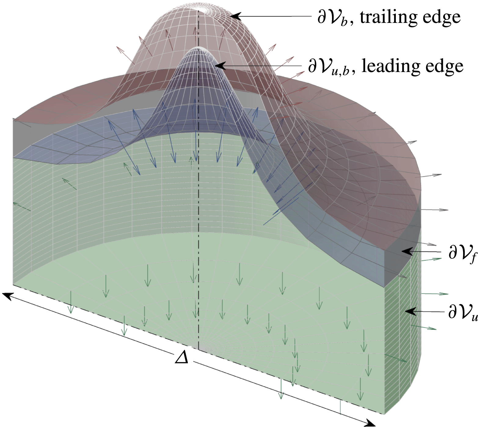
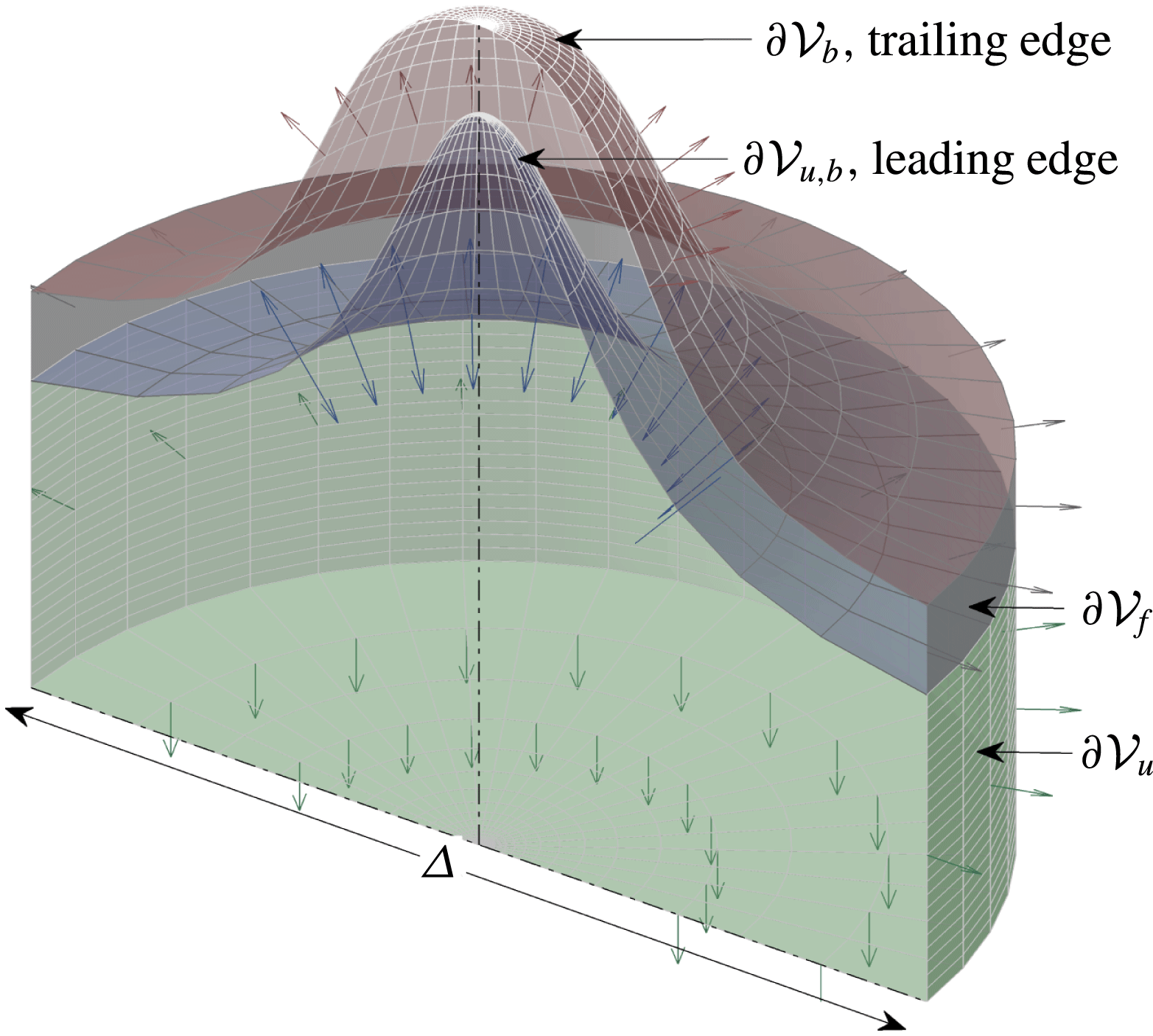
Schematic of (half) the material volume of diameter
 $\unicode[STIX]{x1D6E5}$
, over which (3.1) is integrated. The volume
 ${\mathcal{V}}$
is divided into two parts, i.e.
 ${\mathcal{V}}={\mathcal{V}}_{u}+{\mathcal{V}}_{b}$
with boundaries
 $\unicode[STIX]{x2202}{\mathcal{V}}=\unicode[STIX]{x2202}{\mathcal{V}}_{u}+\unicode[STIX]{x2202}{\mathcal{V}}_{b}+\unicode[STIX]{x2202}{\mathcal{V}}_{f}$
. The two volumes share a common frontier
 $\unicode[STIX]{x2202}{\mathcal{V}}_{u,b}$
. The vectors
 $\boldsymbol{n}$
normal to the different boundaries are indicated by arrows.
3.2 Simplified (measurable) expression
A schematic of the control volume
 ${\mathcal{V}}$
is presented in figure 2.
 ${\mathcal{V}}$
is decomposed into two volumes
 ${\mathcal{V}}_{u}$
and
 ${\mathcal{V}}_{b}$
which are characterized below.
-
(i) The volume
${\mathcal{V}}_{u}$
is the volume enclosed between boundaries
$\unicode[STIX]{x2202}{\mathcal{V}}_{u}$
and
$\unicode[STIX]{x2202}{\mathcal{V}}_{u,b}$
. It covers all the fresh gases (
$\unicode[STIX]{x1D70C}=\unicode[STIX]{x1D70C}_{u}$
,
$Y_{f}^{\ast }=1$
) until the leading edge of the flame
$\unicode[STIX]{x2202}{\mathcal{V}}_{u,b}$
where
$Y_{f}^{\ast }=1$
. The boundary
$\unicode[STIX]{x2202}{\mathcal{V}}_{u}$
is static so that
$\boldsymbol{w}\boldsymbol{\cdot }\boldsymbol{n}=0$
. We also impose
$\boldsymbol{v}_{f}\boldsymbol{\cdot }\boldsymbol{n}=0$
at
$\unicode[STIX]{x2202}{\mathcal{V}}_{u}$
and
$\unicode[STIX]{x2202}{\mathcal{V}}_{u,b}$
, i.e. zero gradient of
$Y_{f}^{\ast }$
at the boundaries. -
(ii) The volume
${\mathcal{V}}_{b}$
is the volume enclosed between boundaries
$\unicode[STIX]{x2202}{\mathcal{V}}_{b}$
,
$\unicode[STIX]{x2202}{\mathcal{V}}_{u,b}$
and
$\unicode[STIX]{x2202}{\mathcal{V}}_{f}$
. It comprises the flame volume from the leading edge
$\unicode[STIX]{x2202}{\mathcal{V}}_{u,b}$
where
$\unicode[STIX]{x1D70C}=\unicode[STIX]{x1D70C}_{u}$
,
$Y_{f}^{\ast }=1$
to the trailing edge
$\unicode[STIX]{x2202}{\mathcal{V}}_{b}$
where
$\unicode[STIX]{x1D70C}\approx \unicode[STIX]{x1D70C}_{b}$
and
$Y_{f}^{\ast }=0$
. Therefore,
$\unicode[STIX]{x0222F}_{\unicode[STIX]{x2202}{\mathcal{V}}_{b}}\unicode[STIX]{x1D70C}Y_{f}^{\ast }(\boldsymbol{u}-\boldsymbol{w}+\boldsymbol{v}_{f})\boldsymbol{\cdot }\boldsymbol{n}=0$
since
$Y_{f}^{\ast }$
is zero at the level of
$\unicode[STIX]{x2202}{\mathcal{V}}_{b}$
. The flux at the boundary
$\unicode[STIX]{x2202}{\mathcal{V}}_{f}$
will be determined later.





With this definition of
 ${\mathcal{V}}$
, equation (3.9) can be further simplified by integrating (3.9) over
 ${\mathcal{V}}_{u}$
and then proceed to the integration over the volume
 ${\mathcal{V}}_{b}$
.
3.2.1 Integration over
${\mathcal{V}}_{u}$

In the unburned gases volume
 ${\mathcal{V}}_{u}$
, we have
 $\unicode[STIX]{x1D70C}=\unicode[STIX]{x1D70C}_{u}$
and
 $Y_{f}^{\ast }=1$
together with
 $\unicode[STIX]{x1D714}_{f}^{\ast }=0$
everywhere. Therefore, (3.9) writes
 $$\begin{eqnarray}\displaystyle \text{MV}|_{{\mathcal{V}}_{u}}+\text{MF}|_{{\mathcal{V}}_{u}} & = & \displaystyle \unicode[STIX]{x1D70C}_{u}\frac{\text{d}}{\text{d}t}\iiint _{{\mathcal{V}}_{u}(t)}\,\text{d}^{3}V+\unicode[STIX]{x1D70C}_{u}\unicode[STIX]{x0222F}_{\unicode[STIX]{x2202}{\mathcal{V}}_{u}(t)}\boldsymbol{u}\boldsymbol{\cdot }\boldsymbol{n}\,\text{d}^{2}A+\unicode[STIX]{x1D70C}_{u}\unicode[STIX]{x0222F}_{\unicode[STIX]{x2202}{\mathcal{V}}_{u,b}(t)}\underbrace{(\boldsymbol{u}-\boldsymbol{w})\boldsymbol{\cdot }\boldsymbol{n}}_{S_{d}^{u}}\,\text{d}^{2}A\nonumber\\ \displaystyle & = & \displaystyle \unicode[STIX]{x1D70C}_{u}\frac{\text{d}{\mathcal{V}}_{u}}{\text{d}t}+\unicode[STIX]{x1D70C}_{u}\unicode[STIX]{x0222F}_{\unicode[STIX]{x2202}{\mathcal{V}}_{u}(t)}\boldsymbol{u}\boldsymbol{\cdot }\boldsymbol{n}\,\text{d}^{2}A+\unicode[STIX]{x1D70C}_{u}\langle S_{d}^{u}\rangle A_{f}=0.\end{eqnarray}$$
The budget in the unburned volume
 ${\mathcal{V}}_{u}$
yields an expression for the area-weighted displacement speed
 $\langle S_{d}^{u}\rangle =\langle (\boldsymbol{u}-\boldsymbol{w})\boldsymbol{\cdot }\boldsymbol{n}\rangle$
(note that in this case
 $\boldsymbol{n}$
is directed towards the burned gases)
 $$\begin{eqnarray}\displaystyle \langle S_{d}^{u}\rangle =\underbrace{-\frac{1}{A_{f}}\frac{\text{d}{\mathcal{V}}_{u}}{\text{d}t}}_{{\mathcal{U}}_{MV}|_{{\mathcal{V}}_{u}}}\underbrace{-\frac{1}{A_{f}}\unicode[STIX]{x0222F}_{\unicode[STIX]{x2202}{\mathcal{V}}_{u}(t)}\boldsymbol{u}\boldsymbol{\cdot }\boldsymbol{n}\,\text{d}^{2}A}_{{\mathcal{U}}_{MF}|_{{\mathcal{V}}_{u}}}. & & \displaystyle\end{eqnarray}$$
The superscript
 $u$
has been kept for designating
 $S_{d}^{u}$
as it corresponds to the displacement speed of the leading edge
 $\unicode[STIX]{x2202}{\mathcal{V}}_{u,b}$
.
 $A_{f}$
is defined as the area of
 $\unicode[STIX]{x2202}{\mathcal{V}}_{u,b}$
, i.e. the area of the leading edge. (It was checked from the present measurements and DNSs that translating the leading edge spatial coordinates in the normal direction of a distance equivalent to the flame thickness did not lead to substantial difference in
 $A_{f}$
. This is indicative that
 $|\boldsymbol{J}|=1$
is plausible in this case.) The terms
 ${\mathcal{U}}_{MV}|_{{\mathcal{V}}_{u}}$
and
 ${\mathcal{U}}_{MF}|_{{\mathcal{V}}_{u}}$
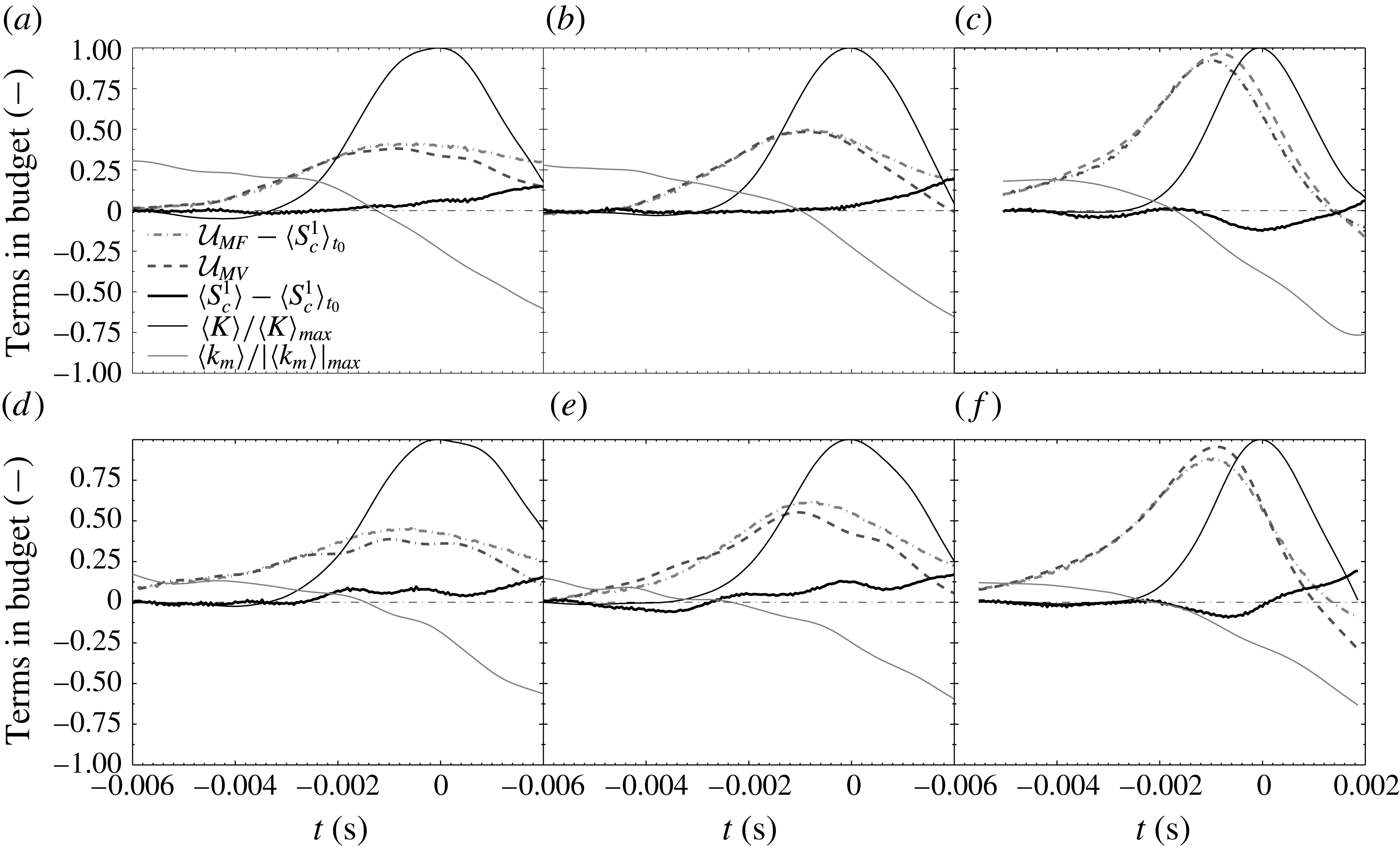
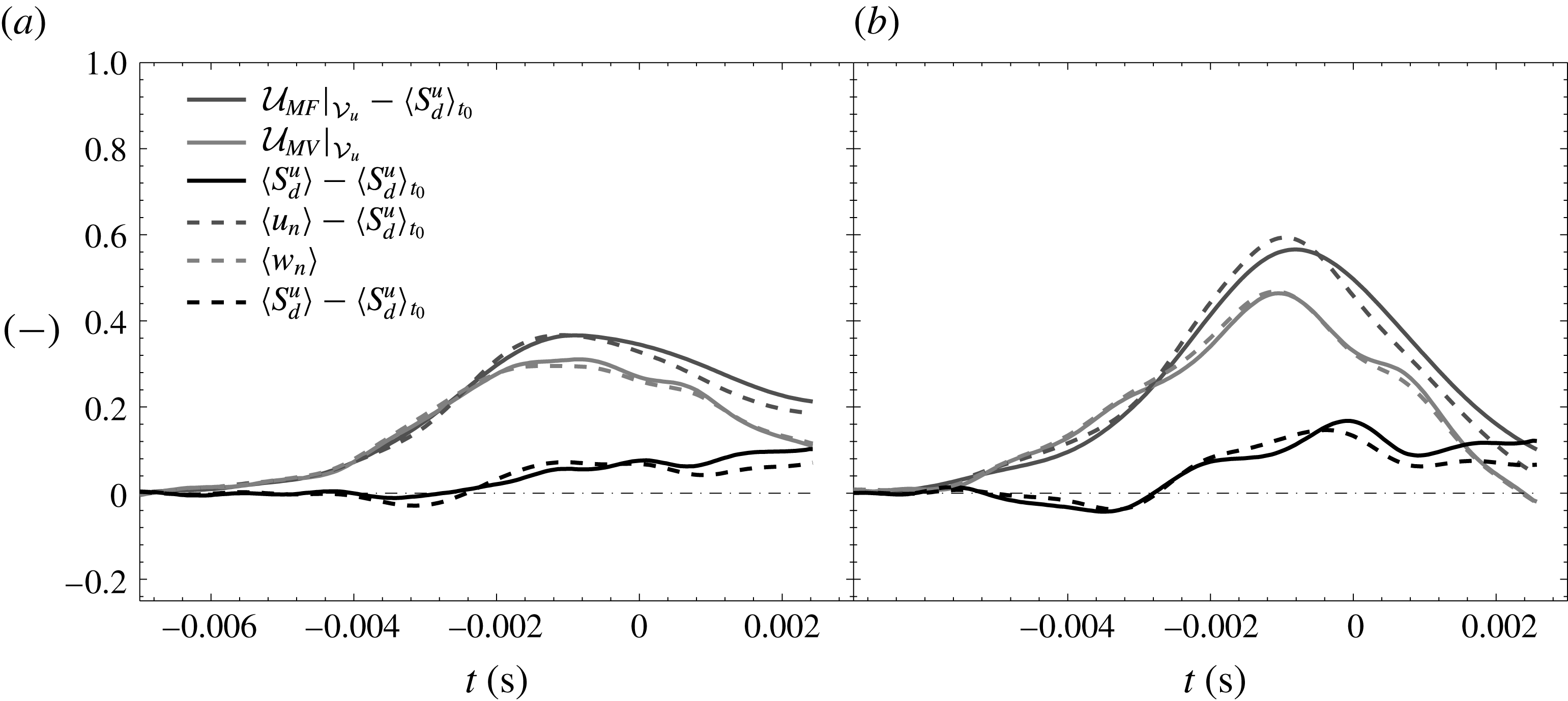
are introduced only for illustrative purposes, and will be useful later when plotting figures 8 and 11.
3.2.2 Integration over
${\mathcal{V}}_{b}$

The MV term integrated over
 ${\mathcal{V}}_{b}$
cannot be measured as we have no information about
 $Y_{f}^{\ast }$
and
 $\unicode[STIX]{x1D70C}$
in the flame. One solution consists in considering an infinitely thin flame so that the time derivative of the integral over
 ${\mathcal{V}}_{b}$
is negligible compared to that over
 ${\mathcal{V}}_{u}$
. Consequently, neglecting the mass within the flame leads to
 $$\begin{eqnarray}\displaystyle \text{MV}|_{{\mathcal{V}}_{b}}=0. & & \displaystyle\end{eqnarray}$$
Another solution consists in expressing the volume integral appearing in
 $\text{MV}|_{{\mathcal{V}}_{b}}$
in the flame curvilinear basis (with again
 $|\boldsymbol{J}|=1$
)
 $$\begin{eqnarray}\displaystyle \iiint _{{\mathcal{V}}_{b}(t)}\unicode[STIX]{x1D70C}Y_{f}^{\ast }\,\text{d}^{3}V=\iint _{A_{f}}\underbrace{\left[\int _{\unicode[STIX]{x1D702}(Y_{f}^{\ast }=0)}^{\unicode[STIX]{x1D702}(Y_{f}^{\ast }=1)}\unicode[STIX]{x1D70C}Y_{f}^{\ast }\,\text{d}\unicode[STIX]{x1D702}\right]}_{\unicode[STIX]{x1D70C}_{u}{\mathcal{F}}}\,\text{d}^{2}A_{f}. & & \displaystyle\end{eqnarray}$$
Then, following Poinsot & Veynante (Reference Poinsot and Veynante2005), one can take the mean value of each variable within the integral, viz.
 $$\begin{eqnarray}\displaystyle {\mathcal{F}}=\frac{1}{\unicode[STIX]{x1D70C}_{u}}\left(\frac{\unicode[STIX]{x1D70C}_{u}+\unicode[STIX]{x1D70C}_{b}}{2}\right)\left(\frac{Y_{f,u}^{\ast }+Y_{f,b}^{\ast }}{2}\right)\unicode[STIX]{x1D6FF}_{L}=\left(1+\frac{\unicode[STIX]{x1D70C}_{b}}{\unicode[STIX]{x1D70C}_{u}}\right)\frac{\unicode[STIX]{x1D6FF}_{L}}{4}, & & \displaystyle\end{eqnarray}$$
where
 $\unicode[STIX]{x1D6FF}_{L}$
is the flame thickness whose appropriate definition may be here
 $\unicode[STIX]{x1D702}(Y_{f}^{\ast }=0.99)-\unicode[STIX]{x1D702}(Y_{f}^{\ast }=0.01)$
. Otherwise, following Poinsot & Veynante (Reference Poinsot and Veynante2011), we can take the average value of
 $\unicode[STIX]{x1D70C}Y_{f}^{\ast }$
, viz.
 $$\begin{eqnarray}\displaystyle {\mathcal{F}}=\frac{1}{\unicode[STIX]{x1D70C}_{u}}\left(\frac{\unicode[STIX]{x1D70C}_{u}Y_{f,u}^{\ast }+\unicode[STIX]{x1D70C}_{b}Y_{f,b}^{\ast }}{2}\right)\unicode[STIX]{x1D6FF}_{L}=\frac{\unicode[STIX]{x1D6FF}_{L}}{2}. & & \displaystyle\end{eqnarray}$$
The mass variation term
 $\text{MV}|_{{\mathcal{V}}_{b}}$
can thus be rewritten as
 $$\begin{eqnarray}\displaystyle \text{MV}|_{{\mathcal{V}}_{b}}=\unicode[STIX]{x1D70C}_{u}\frac{\text{d}\langle {\mathcal{F}}\rangle A_{f}}{\text{d}t}. & & \displaystyle\end{eqnarray}$$
Since we do not have models for
 $\langle {\mathcal{F}}\rangle$
(somehow related to the flame shrinking or thickening) that could emerge from first principles, we will consider
 $\langle {\mathcal{F}}\rangle ={\mathcal{F}}=\text{const}$
. This hypothesis will be tested using DNS of a FVI in section § 4.2. Then,
 $$\begin{eqnarray}\displaystyle \text{MV}|_{{\mathcal{V}}_{b}}=\unicode[STIX]{x1D70C}_{u}{\mathcal{F}}\frac{\text{d}A_{f}}{\text{d}t}. & & \displaystyle\end{eqnarray}$$
Here
 ${\mathcal{F}}=0$
when the contribution of the flame thickness is neglected,
 ${\mathcal{F}}=(1+\unicode[STIX]{x1D70C}_{b}/\unicode[STIX]{x1D70C}_{u})\unicode[STIX]{x1D6FF}_{L}/4$
(Poinsot & Veynante Reference Poinsot and Veynante2005) or
 ${\mathcal{F}}=\unicode[STIX]{x1D6FF}_{L}/2$
(Poinsot & Veynante Reference Poinsot and Veynante2011). CHEMKIN simulations indicate that
 ${\mathcal{F}}=\unicode[STIX]{x1D6FF}_{L}/2$
is more suited than
 ${\mathcal{F}}=(1+\unicode[STIX]{x1D70C}_{b}/\unicode[STIX]{x1D70C}_{u})\unicode[STIX]{x1D6FF}_{L}/4$
. It is worth further emphasizing that
 $\unicode[STIX]{x1D70C}_{b}$
is not measured. This parameter needs thus to be estimated a priori from equilibrium calculations which rely on some assumptions such as flame adiabaticity that might not be accurate in general. Some other authors (Bradley et al.
Reference Bradley, Gaskell and Gu1996) have proposed a different hypothesis for assessing
 ${\mathcal{F}}$
but it relies on an estimation of
 $\unicode[STIX]{x1D70C}_{b}$
and is thus not treated here for the same reason. We will hereafter consider only cases where
 ${\mathcal{F}}=0$
or
 ${\mathcal{F}}=\unicode[STIX]{x1D6FF}_{L}/2$
that will be tested by DNS in § 4.2. It is worth stressing that the present method, where use is made of
 ${\mathcal{F}}=\unicode[STIX]{x1D6FF}_{L}/2=\text{const.}$
is thus not suitable when there is significant flame extinction or large variations of flame thickness. It is restricted to the flamelet regime of combustion. Note however that the integral approach for measuring
 $\langle S_{d}^{u}\rangle$
does not require any hypothesis regarding the flame structure and can thus be used irrespective of the combustion regime. The integral approach depends on ad hoc coefficients for inferring the mass contained within the flame that can, at best, be estimated. Different estimates may yield different conclusions; this is in contrast to the asymptotic derivation that provides a solution with no undetermined coefficients.
The MF term integrated over
 ${\mathcal{V}}_{b}$
leads to
 $$\begin{eqnarray}\displaystyle \text{MF}|_{{\mathcal{V}}_{b}} & = & \displaystyle \unicode[STIX]{x0222F}_{\unicode[STIX]{x2202}{\mathcal{V}}_{u,b}(t)+\unicode[STIX]{x2202}{\mathcal{V}}_{f}(t)}[\unicode[STIX]{x1D70C}Y_{f}^{\ast }(\boldsymbol{u}+\boldsymbol{v}_{f}-\boldsymbol{w})\boldsymbol{\cdot }\boldsymbol{n}]\,\text{d}^{2}A\nonumber\\ \displaystyle & = & \displaystyle \unicode[STIX]{x1D70C}_{u}\unicode[STIX]{x0222F}_{\unicode[STIX]{x2202}{\mathcal{V}}_{u,b}}\underbrace{(\boldsymbol{u}-\boldsymbol{w})\boldsymbol{\cdot }\boldsymbol{n}}_{-S_{d}^{u}}\,\text{d}^{2}A+\unicode[STIX]{x0222F}_{\unicode[STIX]{x2202}{\mathcal{V}}_{f}}[\unicode[STIX]{x1D70C}Y_{f}^{\ast }(\boldsymbol{u}+\boldsymbol{v}_{f}-\boldsymbol{w})\boldsymbol{\cdot }\boldsymbol{n}]\,\text{d}^{2}A\nonumber\\ \displaystyle & = & \displaystyle -\unicode[STIX]{x1D70C}_{u}\langle S_{d}^{u}\rangle A_{f}+\unicode[STIX]{x0222F}_{\unicode[STIX]{x2202}{\mathcal{V}}_{f}}[\unicode[STIX]{x1D70C}Y_{f}^{\ast }(\boldsymbol{u}+\boldsymbol{v}_{f}-\boldsymbol{w})\boldsymbol{\cdot }\boldsymbol{n}]\,\text{d}^{2}A.\end{eqnarray}$$
Here, we neglect the diffusion velocity
 $\boldsymbol{v}_{f}\boldsymbol{\cdot }\boldsymbol{n}$
at the boundary
 $\unicode[STIX]{x2202}{\mathcal{V}}_{f}$
assuming that the species gradient is oriented in the flame normal direction. Second, we have
 $\boldsymbol{w}\boldsymbol{\cdot }\boldsymbol{n}=0$
at
 $\unicode[STIX]{x2202}{\mathcal{V}}_{f}$
. Finally, we take the average value of
 $\unicode[STIX]{x1D70C}Y_{f}^{\ast }\boldsymbol{u}\boldsymbol{\cdot }\boldsymbol{n}$
between the burned and fresh regions to obtain:
 $$\begin{eqnarray}\displaystyle \unicode[STIX]{x0222F}_{\unicode[STIX]{x2202}{\mathcal{V}}_{f}}\unicode[STIX]{x1D70C}Y_{f}^{\ast }\boldsymbol{u}\boldsymbol{\cdot }\boldsymbol{n}=\frac{\unicode[STIX]{x1D70C}_{u}Y_{f,u}^{\ast }v_{r,u}+\unicode[STIX]{x1D70C}_{b}Y_{f,b}^{\ast }v_{r,b}}{2}\unicode[STIX]{x03C0}\unicode[STIX]{x0394}\unicode[STIX]{x1D6FF}_{L}, & & \displaystyle\end{eqnarray}$$
where
 $v_{r,u}$
and
 $v_{r,b}$
is the fluid velocity tangential to the flame at the level of
 $\unicode[STIX]{x2202}{\mathcal{V}}_{f}$
(whose area is equal to
 $\unicode[STIX]{x03C0}\unicode[STIX]{x0394}\unicode[STIX]{x1D6FF}_{L}$
,
 $\unicode[STIX]{x1D6E5}$
is the diameter of the control volume), in the fresh and burned gases, respectively. Recalling that
 $Y_{f,b}^{\ast }=0$
, we end up with
 $$\begin{eqnarray}\displaystyle \text{MF}|_{{\mathcal{V}}_{b}}=-\unicode[STIX]{x1D70C}_{u}\langle S_{d}^{u}\rangle A_{f}+\unicode[STIX]{x1D70C}_{u}{\mathcal{F}}\unicode[STIX]{x03C0}\unicode[STIX]{x0394}v_{r,u}. & & \displaystyle\end{eqnarray}$$
With these simplifications, the integration of the mass budget (3.9) over
 ${\mathcal{V}}_{b}$
leads to
 $$\begin{eqnarray}\displaystyle \langle S_{c}\rangle =\langle S_{d}^{u}\rangle -{\mathcal{F}}\left(\frac{1}{A_{f}}\frac{\text{d}A_{f}}{\text{d}t}+\frac{1}{A_{f}}\unicode[STIX]{x03C0}\unicode[STIX]{x0394}v_{r,u}\right), & & \displaystyle\end{eqnarray}$$
or equivalently by using (3.11) for
 $\langle S_{d}^{u}\rangle$
 $$\begin{eqnarray}\displaystyle \langle S_{c}\rangle =\underbrace{-A_{f}^{-1}\left(\frac{\text{d}{\mathcal{V}}_{u}}{\text{d}t}+{\mathcal{F}}\frac{\text{d}A_{f}}{\text{d}t}\right)}_{{\mathcal{U}}_{MV}}\underbrace{-A_{f}^{-1}\left(\unicode[STIX]{x0222F}_{\unicode[STIX]{x2202}{\mathcal{V}}_{u}}\boldsymbol{u}\boldsymbol{\cdot }\boldsymbol{n}\,\text{d}^{2}A+{\mathcal{F}}\unicode[STIX]{x03C0}\unicode[STIX]{x0394}v_{r,u}\right)}_{{\mathcal{U}}_{MF}}. & & \displaystyle\end{eqnarray}$$
The
 ${\mathcal{U}}_{MV}$
term in (3.22) is sometimes referred to as the mass accumulation process while the
 ${\mathcal{U}}_{MF}$
term represents the net mass flux flowing through the system. Note that the consumption speed evaluated by considering the thin flame limit (
 ${\mathcal{F}}=0$
) is equal to the displacement speed
 $\langle S_{d}^{u}\rangle$
. Hereafter, we will note
 $\langle S_{c}^{0}\rangle =\langle S_{d}^{u}\rangle$
the consumption speed inferred with
 ${\mathcal{F}}=0$
and
 $\langle S_{c}^{1}\rangle$
that calculated with
 ${\mathcal{F}}=\unicode[STIX]{x1D6FF}_{L}/2$
. It is worth stressing that (3.21) highlights an explicit relationship between displacement speed (at the leading edge) and consumption speed and shows that the differences between
 $\langle S_{c}\rangle$
and
 $\langle S_{d}^{u}\rangle$
are connected to the mass contained within the flame and to the total stretch rate
 $1/A_{f}\,\text{d}A_{f}/\text{d}t$
. Another discrepancy between the behaviour of
 $\langle S_{c}\rangle$
and
 $\langle S_{d}^{u}\rangle$
relies on the tangential mass flux (through the appearance of
 $v_{r,u}$
, the tangential velocity) leaving the flame.
4 Experimental and numerical validation
4.1 Experimental validation at steady state
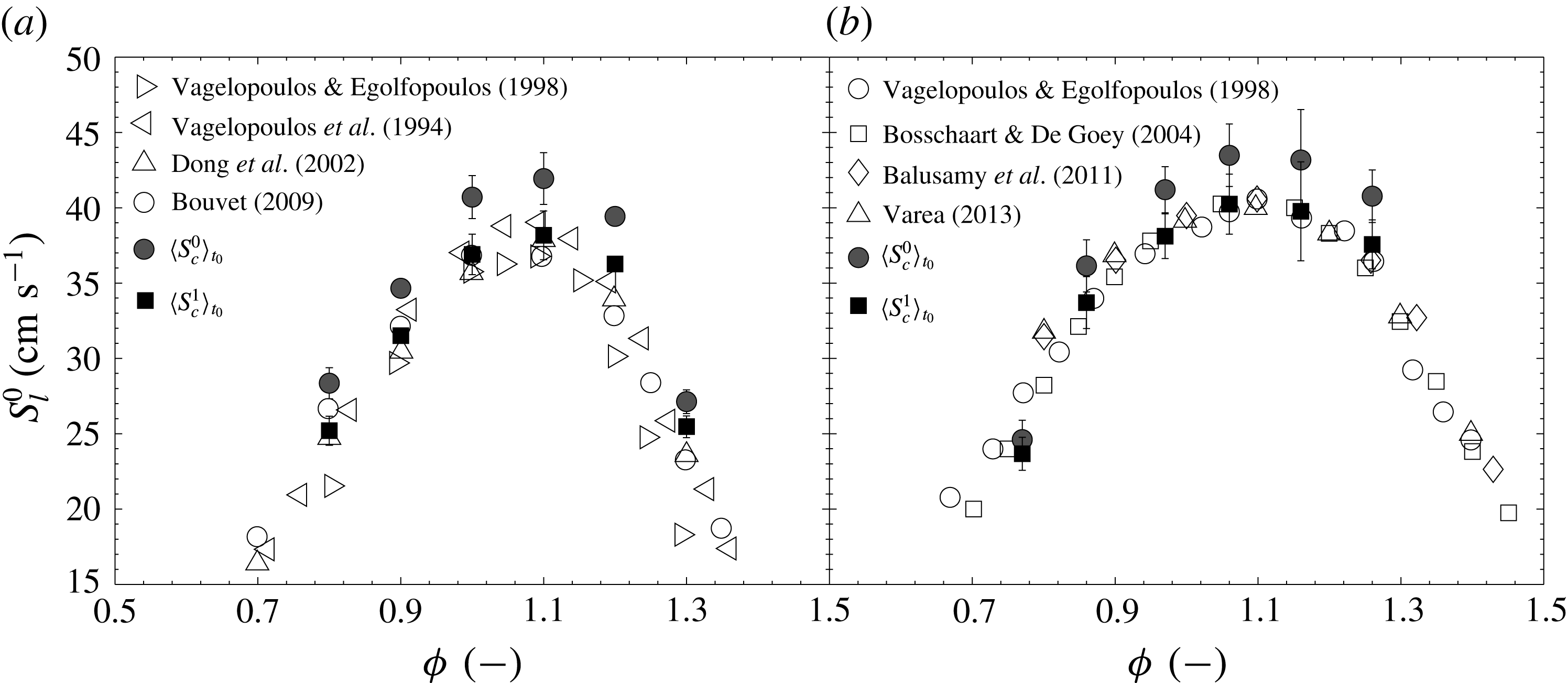
Comparison of the present experimental assessment of the consumption speed using (4.1) with
 ${\mathcal{F}}=0$
(filled circle) and
 ${\mathcal{F}}=\unicode[STIX]{x1D6FF}_{L}/2$
(filled square), for methane (a) and propane/air mixtures (b) at different equivalence ratios
 $\unicode[STIX]{x1D719}$
with data from the literature. Error bars correspond to the standard deviation calculated from 15 independent measurements. Experimental data are taken from Vagelopoulos et al. (Reference Vagelopoulos, Egolfopoulos and Law1994), Vagelopoulos & Egolfopoulos (Reference Vagelopoulos and Egolfopoulos1998), Dong et al. (Reference Dong, Vagelopoulos, Spedding and Egolfopoulos2002), Bosschaart & De Goey (Reference Bosschaart and De Goey2004), Bouvet (Reference Bouvet2009), Balusamy et al. (Reference Balusamy, Cessou and Lecordier2011) and Varea (Reference Varea2013).

When the flame is stationary (no vortex), the time derivatives are zero in (3.22) and therefore, the consumption speed at steady state (noted
 $\langle S_{c}\rangle _{t_{0}}$
) writes
 $$\begin{eqnarray}\displaystyle \langle S_{c}\rangle _{t_{0}}=-A_{f}^{-1}\left(\unicode[STIX]{x0222F}_{\unicode[STIX]{x2202}{\mathcal{V}}_{u}}\boldsymbol{u}\boldsymbol{\cdot }\boldsymbol{n}\,\text{d}^{2}A+{\mathcal{F}}\unicode[STIX]{x03C0}\unicode[STIX]{x0394}v_{r,u}\right). & & \displaystyle\end{eqnarray}$$
Again,
 $A_{f}$
is inferred from the measurements and thus corresponds to an isotherm located rather close to the unburned gases. Supposing a disc shaped flame, we have
 $A_{f}=\unicode[STIX]{x03C0}\unicode[STIX]{x1D6E5}^{2}/4$
. By further noting that the tangential velocity evolves linearly with
 $\unicode[STIX]{x1D6E5}$
, i.e.
 $v_{r,u}=K_{r}\unicode[STIX]{x1D6E5}/2$
(
 $K_{r}$
being the tangential strain rate)
 $$\begin{eqnarray}\displaystyle \langle S_{c}^{1}\rangle _{t_{0}}=\langle S_{c}^{0}\rangle _{t_{0}}-2{\mathcal{F}}K_{r}, & & \displaystyle\end{eqnarray}$$
which indicates that the error which is made on
 $\langle S_{c}\rangle$
assuming
 ${\mathcal{F}}=0$
is proportional to both the flame thickness
 $\unicode[STIX]{x1D6FF}_{L}$
and the tangential strain rate
 $K_{r}$
. Considering a linear dependence of
 $\langle S_{c}\rangle$
to
 $K_{r}$
through the Markstein length
 ${\mathcal{L}}$
, it can be shown that
 $$\begin{eqnarray}\displaystyle {\mathcal{L}}^{1}={\mathcal{L}}^{0}-2{\mathcal{F}}. & & \displaystyle\end{eqnarray}$$
As first pointed out by Poinsot (Reference Poinsot1998), the error on
 ${\mathcal{L}}$
when considering
 ${\mathcal{F}}=0$
is of the order of the flame thickness and can even change its sign.
As a first validation, we will focus on the estimation of
 $\langle S_{c}^{0}\rangle _{t_{0}}$
(zero flame thickness) and
 $\langle S_{c}^{1}\rangle _{t_{0}}$
(finite flame thickness), for methane/air and propane/air mixtures. Even though the flames considered here are strained, we compare directly our estimates to
 $S_{l}^{0}$
, i.e. the extrapolated value of
 $S_{c}$
or
 $S_{d}^{u}$
to zero stretch rate generally reported in papers. This seems reasonable for the low values of the strain rate measured in our experiments,
 $K_{r}$
being approximately 80. Results (figure 3) indicate a substantial difference between
 $\langle S_{c}^{1}\rangle _{t_{0}}$
and
 $\langle S_{c}^{0}\rangle _{t_{0}}$
, with
 $\langle S_{c}^{1}\rangle _{t_{0}}$
being systematically closer to experimental data taken from the literature. The contribution of the mass flow rate through
 $\unicode[STIX]{x2202}{\mathcal{V}}_{f}$
is between 7 % and 10 % depending on the type of fuel and equivalence ratio. Present estimates of
 $\langle S_{c}^{1}\rangle _{t_{0}}$
are in excellent agreement with experimental data from the literature. The small differences that are observed are about 5 % which may be attributed to experimental uncertainties and the effect of stretch.
These first tests show that the present method is reliable for measuring the flame consumption speed at least at stationary state. Second, the zero flame thickness assumption (
 ${\mathcal{F}}=0$
) appears to be inadequate and the improvement provided by assuming
 ${\mathcal{F}}=\unicode[STIX]{x1D6FF}_{L}/2$
is significant and provides trustworthy results.
4.2 Numerical validation
Before proceeding with the numerical validation, it is worth stressing that the DNSs are employed with the aim of assessing the adequacy of the hypothesis invoked when deriving (3.22). Therefore, only a stoichiometric methane flame is considered in the DNS. Our goal was not to carry out a quantitative comparison between DNS and experiments. In the experiments, the flame is indeed axisymmetric in contrast with the DNS for which it is planar. The azimuthal curvature component
 $\unicode[STIX]{x1D705}_{2}$
(which is of same order of magnitude than
 $\unicode[STIX]{x1D705}_{1}$
in our experimental configuration) is thus zero in the DNS leading to much smaller mean curvature magnitude. We just aim at guaranteeing that the DNS and experimental observations remain qualitatively similar. i.e. that combustion lies in the same regime. This is ensured by investigating FVIs at approximatively the same
 $U_{\unicode[STIX]{x1D703}}/\langle S_{c}\rangle _{t_{0}}$
and
 $R_{v}/\unicode[STIX]{x1D6FF}_{th}$
between the experiments and the simulation. The objective is the evaluation of the accuracy of (3.22), regardless of the flame configuration. If invalidated in two dimensions, it cannot be used. Conversely, its accuracy in 2-D FVI is an indication that it can be used in an axisymmetric FVI.
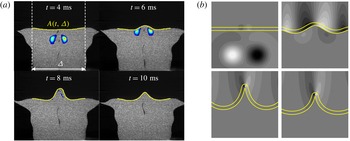
Typical experimental and numerical images of FVI are portrayed in figure 4. In a first phase, the vortex is simply convected towards the flame. In the experiments (figure 4 a), the flame is rather flat throughout this period suggesting that the vortex generator is sufficiently far from the burner outlet for not creating a wake. While advancing, the vortex starts interacting with the flame whose surface increases. The vortex then crosses the flame front, the flame area reaches a maximum before dropping as the flame goes back to its original position. The flame shape and corrugation magnitude appear to be qualitatively similar in the DNS and experiments indicating that these FVIs lie in the same combustion regime.
The flame thickness (identified in the DNS fields by the two fuel mass fraction iso-levels
 $Y_{f}^{\ast }=0.01$
and
 $Y_{f}^{\ast }=0.99$
) remains constant during the interaction with the vortex (figure 4
b), confirming the adequacy of the present assumption regarding
 ${\mathcal{F}}$
. This can be more rigorously verified by calculating the fuel mass contained within the flame and comparing it to the proposed model, viz.
 $$\begin{eqnarray}\displaystyle \iiint _{{\mathcal{V}}_{b}}\unicode[STIX]{x1D70C}Y_{f}^{\ast }\,\text{d}^{3}V\overset{?}{=}\unicode[STIX]{x1D70C}_{u}\langle {\mathcal{F}}\rangle A_{f}, & & \displaystyle\end{eqnarray}$$
where
 ${\mathcal{V}}_{b}$
is the volume comprised between
 $Y_{f}^{\ast }=0.01$
and
 $Y_{f}^{\ast }=0.99$
. Similarly to experiments,
 $A_{f}$
is the flame area of the leading edge here defined as the
 $Y_{f}^{\ast }=0.01$
iso-level. Second, we also have to check whether
 ${\mathcal{F}}$
is constant in time or if the flame is thickened or shrunk. The latter hypothesis arises when simplifying (3.16) to (3.17). Finally, the ratio
 ${\mathcal{F}}/\unicode[STIX]{x1D6FF}_{L}$
itself needs to be determined.
Time sequence of FVI. (a) Experimental contour of vorticity superimposed on the raw Mie scattering image together with one particular isotherm located close to the leading edge. (b) DNS contours of vorticity and the
 $Y_{f}^{\ast }=0.01$
and
 $Y_{f}^{\ast }=0.99$
iso-levels. For clarity, the DNS field has been symmetrically doubled and only a portion of the calculation domain is displayed in (b).

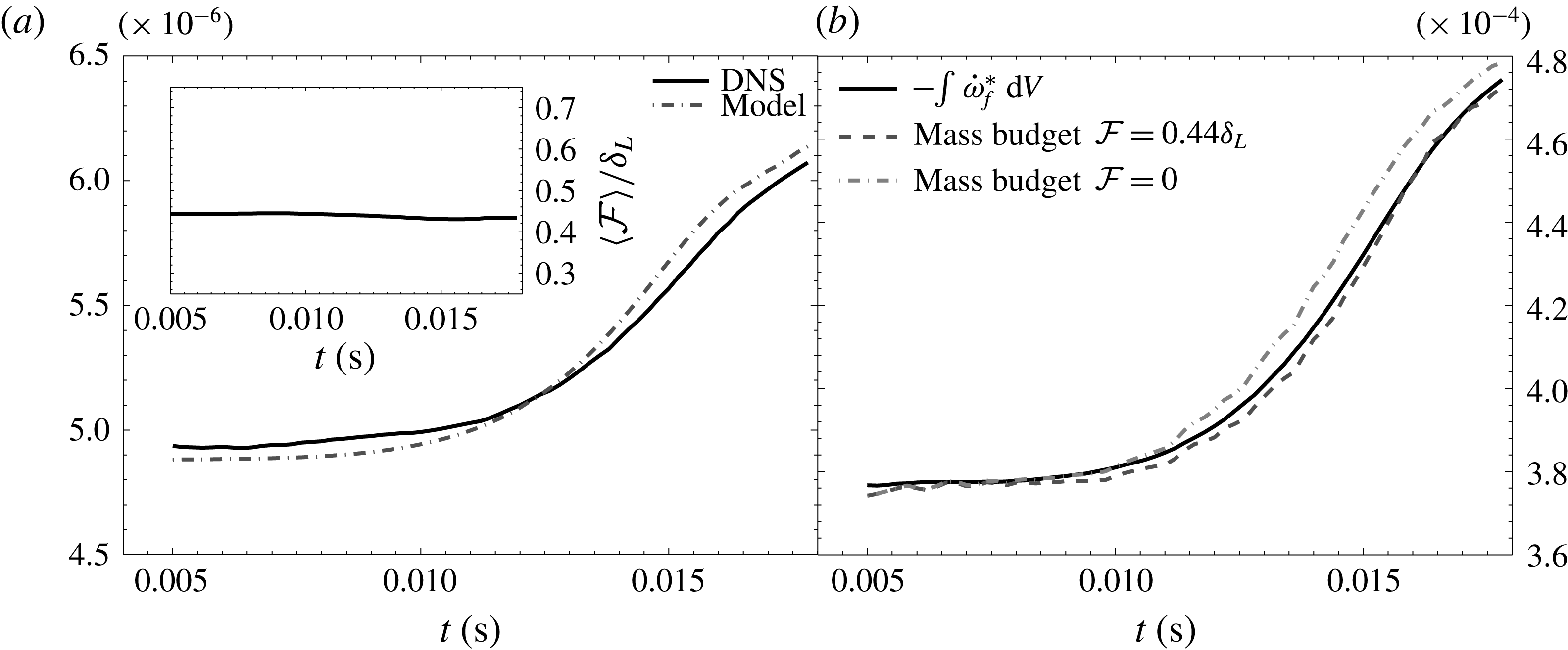
(a) Time evolution of the mass contained within the flame as inferred from the DNS (left-hand side of (4.4)) or the model with
 ${\mathcal{F}}=\text{const.}=0.44\unicode[STIX]{x1D6FF}_{L}$
(right-hand side of (4.4)). The figure in the inset represents the ratio
 ${\mathcal{F}}/\unicode[STIX]{x1D6FF}_{L}$
. (b) Volume integrated fuel reaction rate as inferred from the DNS, compared with the mass budget using either
 ${\mathcal{F}}=0$
or
 ${\mathcal{F}}=\text{const.}=0.44\unicode[STIX]{x1D6FF}_{L}$
. Using
 ${\mathcal{F}}=\text{const.}=0.5\unicode[STIX]{x1D6FF}_{L}$
was undistinguishable from
 ${\mathcal{F}}=\text{const.}=0.44\unicode[STIX]{x1D6FF}_{L}$
.

Results are presented in figure 5(a) where we first test the validity of (4.4). The mass within the flame is inferred from DNS and compared to the model of Poinsot & Veynante (Reference Poinsot and Veynante2011) using
 ${\mathcal{F}}=\text{const.}$
. One observes very marginal differences between the model and the DNS suggesting that
 ${\mathcal{F}}=\text{const.}$
is appropriate. This is further confirmed by plotting the ratio
 ${\mathcal{F}}/\unicode[STIX]{x1D6FF}_{L}$
as a function of time (inset in 5
a) which appears to be nearly constant. The flame zone is thus only very weakly affected by thickening or shrinking effects which are moderate in our case. The average value for
 ${\mathcal{F}}$
is about
 $0.44\unicode[STIX]{x1D6FF}_{L}$
which is in fairly good agreement with the expected theoretical value of
 $0.5\unicode[STIX]{x1D6FF}_{L}$
.
An overall test of (3.22) is also portrayed in figure 5(b). The volume integrated fuel reaction rate is compared to the one calculated by
 $\unicode[STIX]{x1D70C}_{u}\langle S_{c}\rangle A_{f}$
, where
 $\langle S_{c}\rangle$
is calculated from (3.22). A fairly good agreement is observed thus validating the proposed assumptions. The reaction rate measured assuming
 ${\mathcal{F}}=0$
is also displayed indicating that a good estimation of the mass (
 ${\mathcal{F}}=0.44\unicode[STIX]{x1D6FF}_{L}$
) within the flame thickness is mandatory for accurately estimating the fuel consumption speed.
5 Geometric and kinematic features of flame/vortex interactions
Now that the method for assessing
 $\langle S_{c}\rangle$
has been validated, we turn our attention to the effects of different vortex intensities and the effective Lewis number on the flame geometrical and kinematic properties.
5.1 Geometrical features
5.1.1 The total stretch rate
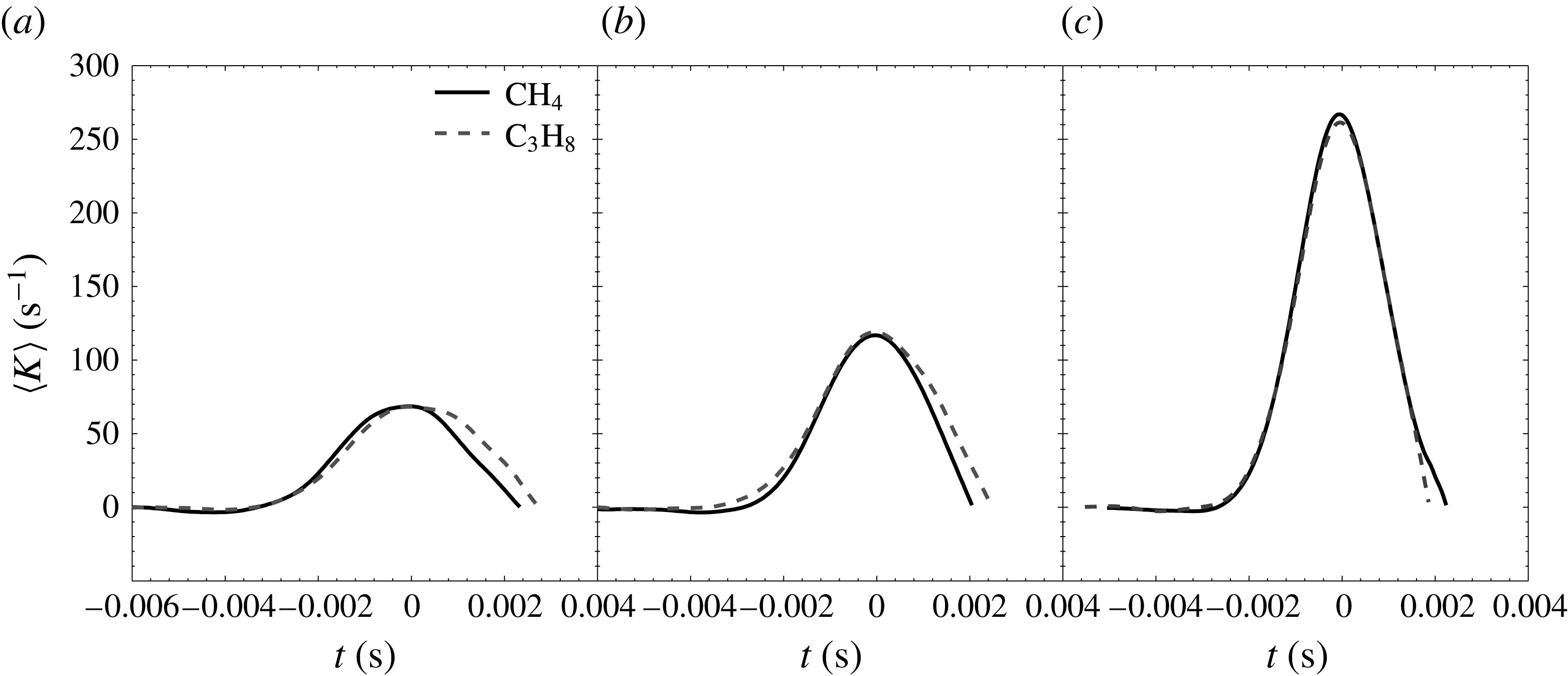
The time evolution of flame area and stretch rate during FVIs are discussed first. Similarly to Thiesset et al. (Reference Thiesset, Maurice, Halter, Mazellier, Chauveau and Gökalp2017), the stretch rate noted
 $\langle K\rangle$
is given in terms of relative increase in flame surface area evaluated over a domain of width
 $\unicode[STIX]{x1D6E5}$
(figure 4
a), viz.
 $$\begin{eqnarray}\displaystyle \langle K(\unicode[STIX]{x1D6E5},t)\rangle =\frac{1}{A_{f}(\unicode[STIX]{x1D6E5},t)}\frac{\text{d}A_{f}(\unicode[STIX]{x1D6E5},t)}{\text{d}t}. & & \displaystyle\end{eqnarray}$$
 $\langle K\rangle$
should be interpreted here as the additional stretch rate due to the interaction with the vortex. Indeed, even when the flame is flat and stationary, stretch is not zero and is simply related to
 $K_{r}$
introduced in (4.2). The total surface-averaged stretch rate
 $\langle K_{tot}\rangle$
over a domain of diameter
 $\unicode[STIX]{x1D6E5}$
is the addition of the stretch rate due to the interaction with the vortex
 $\langle K\rangle$
and that due to the diverging stagnation point flow. It appears explicitly in (3.21) and reads
 $$\begin{eqnarray}\displaystyle \langle K_{tot}\rangle =\frac{1}{A_{f}}\frac{\text{d}A_{f}}{\text{d}t}+\frac{1}{A_{f}}\unicode[STIX]{x03C0}\unicode[STIX]{x0394}v_{r,u}. & & \displaystyle\end{eqnarray}$$
Hereafter, because the variations in time of the rightmost term of the right-hand side of (5.2) are much smaller than that of
 $\langle K\rangle$
, results will be presented as a function of
 $\langle K\rangle$
and not
 $\langle K_{tot}\rangle$
. The stretch rate quantity controls efficiency functions which are widely used in LES of turbulent premixed combustion (Colin et al.
Reference Colin, Ducros, Veynante and Poinsot2000; Charlette et al.
Reference Charlette, Meneveau and Veynante2002; Bougrine et al.
Reference Bougrine, Richard, Colin and Veynante2014; Thiesset et al.
Reference Thiesset, Maurice, Halter, Mazellier, Chauveau and Gökalp2017). It is worth emphasizing that
 $\langle K(\unicode[STIX]{x1D6E5},t)\rangle$
is the area-weighted average of the local stretch rate
 $K=K_{T}+K_{C}$
due to the interaction with the vortex. Indeed, starting from a transport theorem for material surfaces (equation (3) in (Candel & Poinsot Reference Candel and Poinsot1990))
 $$\begin{eqnarray}\displaystyle \frac{\text{d}}{\text{d}t}\int _{A_{f}}\,\text{d}^{2}A=\int _{A_{f}}(-\boldsymbol{n}\boldsymbol{n}:\unicode[STIX]{x1D735}\boldsymbol{u}+\unicode[STIX]{x1D735}\boldsymbol{\cdot }\boldsymbol{u}+2S_{d}\unicode[STIX]{x1D705}_{m})\,\text{d}^{2}A & & \displaystyle\end{eqnarray}$$
or equivalently
 $$\begin{eqnarray}\displaystyle \frac{\text{d}A_{f}}{\text{d}t}=A_{f}\langle K\rangle , & & \displaystyle\end{eqnarray}$$
which yields (5.1). Thiesset et al. (Reference Thiesset, Maurice, Halter, Mazellier, Chauveau and Gökalp2017) showed that the stretch rate also depends on the width
 $\unicode[STIX]{x1D6E5}$
of the domain over which
 $A_{f}$
is measured: obviously for an infinite
 $\unicode[STIX]{x1D6E5}$
, the portion of the flame interacting with the vortex is negligible and
 $\langle K\rangle$
should tend to zero. In other words, because the portion of flame interacting with the vortex is constant (i.e. there exists a
 $\unicode[STIX]{x1D6E5}=\unicode[STIX]{x1D6E5}_{i}$
above which
 $\text{d}A/\text{d}t$
is independent of
 $\unicode[STIX]{x1D6E5}$
), we expect
 $\langle K\rangle$
to decrease with
 $\unicode[STIX]{x1D6E5}^{2}$
since
 $A_{f}(t,\unicode[STIX]{x1D6E5})$
monotonically increases with
 $\unicode[STIX]{x1D6E5}^{2}$
. The evolution of
 $\langle K(\unicode[STIX]{x1D6E5},t)\rangle$
with respect to
 $\unicode[STIX]{x1D6E5}$
can be readily described by the following expression (Thiesset et al.
Reference Thiesset, Maurice, Halter, Mazellier, Chauveau and Gökalp2017)
 $$\begin{eqnarray}\displaystyle \langle K\rangle (\unicode[STIX]{x1D6E5},t)=\langle K_{0}\rangle (t)\left(\frac{\unicode[STIX]{x1D6E5}_{i}-\unicode[STIX]{x1D6E5}_{o}}{\unicode[STIX]{x1D6E5}-\unicode[STIX]{x1D6E5}_{o}}\right)^{2}. & & \displaystyle\end{eqnarray}$$
In (5.5),
 $\unicode[STIX]{x1D6E5}_{i}$
represents the domain width
 $\unicode[STIX]{x1D6E5}$
above which
 $\text{d}A/\text{d}t$
is constant and
 $\unicode[STIX]{x1D6E5}_{0}$
is interpreted as a virtual origin, i.e.
 $\langle K\rangle ^{-1}\rightarrow 0$
when
 $\unicode[STIX]{x1D6E5}\rightarrow \unicode[STIX]{x1D6E5}_{o}$
. Thiesset et al. (Reference Thiesset, Maurice, Halter, Mazellier, Chauveau and Gökalp2017) pointed out that
 $\unicode[STIX]{x1D6E5}_{i}/R_{v}$
and
 $\unicode[STIX]{x1D6E5}_{o}/R_{v}$
(
 $R_{v}$
is the vortex core-to-core distance) were constant irrespectively of the vortex strength and were equal to
 $2.5\pm 0.05$
and
 $-0.5\pm 0.1$
, respectively. In the present study, unless specified, results will be presented for
 $\unicode[STIX]{x1D6E5}=13~\text{mm}$
which corresponds approximatively to
 $\unicode[STIX]{x1D6E5}_{i}$
.
Time evolution of the stretch rate for stoichiometric methane and lean (
 $\unicode[STIX]{x1D719}=0.9$
) propane/air mixtures for three different vortex strengths and
 $\unicode[STIX]{x1D6E5}=13~\text{mm}$
: (a)
 $U_{\unicode[STIX]{x1D703}}/\langle S_{c}^{1}\rangle _{t_{0}}=0.8$
, (b)
 $U_{\unicode[STIX]{x1D703}}/\langle S_{c}^{1}\rangle _{t_{0}}=1.2$
, (c)
 $U_{\unicode[STIX]{x1D703}}/\langle S_{c}^{1}\rangle _{t_{0}}=2.8$
. The time
 $t$
has been shifted so that
 $t=0$
corresponds to the time at which
 $\langle K\rangle$
is maximum.

We consider FVIs for a stoichiometric methane/air mixture characterized by an effective Lewis number close to unity (
 $Le=1.05$
) and a lean (
 $\unicode[STIX]{x1D719}=0.9$
) propane/air mixture for which the Lewis number is about 1.5. The method of Bechtold & Matalon (Reference Bechtold and Matalon2001) was employed for calculating the effective Lewis numbers. Three different vortex strengths are investigated
 $U_{\unicode[STIX]{x1D703}}/\langle S_{c}^{1}\rangle _{t_{0}}=0.8$
, 1.2 and 2.8.
Results (figure 6) indicate that for the range of vortex strengths investigated here, the magnitude of the total stretch rate increases with
 $U_{\unicode[STIX]{x1D703}}/\langle S_{c}^{1}\rangle _{t_{0}}$
. One further notes that there is no significant influence of the Lewis number on the creation of surface area as the time evolution of
 $\langle K\rangle$
is very similar irrespectively of the type of fuel investigated. The vortex efficiency, i.e.
 $\max (\langle K\rangle )/(U_{\unicode[STIX]{x1D703}}/R_{v})$
is equal to 0.73, 0.88 and 1.06 for methane/air flames at
 $U_{\unicode[STIX]{x1D703}}/\langle S_{c}^{1}\rangle _{t_{0}}=0.8$
, 1.2 and 2.8, respectively. For propane/air flames, the stretch efficiency is found to be equal to 0.78, 0.92 and 1.06 for
 $U_{\unicode[STIX]{x1D703}}/\langle S_{c}^{1}\rangle _{t_{0}}=0.8$
, 1.2 and 2.8, respectively. This observation is in agreement with the DNS data of Bougrine et al. (Reference Bougrine, Richard, Colin and Veynante2014), where the differences in stretch rates between
 $\text{CH}_{4}$
and
 $\text{C}_{3}\text{H}_{8}$
were small. This indicates that when considering fuels with
 $Le\geqslant 1$
, Lewis number corrections to the stretch efficiency functions might not be necessary.
As the flame positions (and thus area and stretch) can be computed from a purely kinematic equation (the level-set equation) (Moureau, Fiorina & Pitsch Reference Moureau, Fiorina and Pitsch2009; Thiesset et al.
Reference Thiesset, Maurice, Halter, Mazellier, Chauveau and Gökalp2017), the independence of
 $\langle K\rangle$
to the Lewis number indicates a priori that the evolution of the flame displacement
 $S_{d}$
during a FVI remains similar irrespectively of the Lewis number (at least for
 $Le\geqslant 1$
).
5.1.2 Flame curvature
In addition to (3.11) which provides a means to experimentally assess the area-weighted flame displacement speed, the simultaneous PIV and tomographic measurements allow local values (i.e. as a function of the position on the interface) of
 $S_{d}^{u}$
to be evaluated by (Peters Reference Peters2000; Poinsot & Veynante Reference Poinsot and Veynante2011)
 $$\begin{eqnarray}\displaystyle S_{d}^{u}=(\boldsymbol{w}-\boldsymbol{u})\boldsymbol{\cdot }\boldsymbol{n}=w_{n}-u_{n}=\left.\frac{1}{|\unicode[STIX]{x1D735}\unicode[STIX]{x1D713}|}\left(\frac{\unicode[STIX]{x2202}\unicode[STIX]{x1D713}}{\unicode[STIX]{x2202}t}+\boldsymbol{u}\boldsymbol{\cdot }\unicode[STIX]{x1D735}\unicode[STIX]{x1D713}\right)\right|_{\unicode[STIX]{x1D713}=\unicode[STIX]{x1D713}_{0}}, & & \displaystyle\end{eqnarray}$$
with
 $$\begin{eqnarray}\displaystyle \boldsymbol{n}=-\frac{\unicode[STIX]{x1D735}\unicode[STIX]{x1D713}}{|\unicode[STIX]{x1D735}\unicode[STIX]{x1D713}|}, & & \displaystyle\end{eqnarray}$$
where
 $w_{n}=\boldsymbol{w}\boldsymbol{\cdot }\boldsymbol{n}$
and
 $u_{n}=\boldsymbol{u}\boldsymbol{\cdot }\boldsymbol{n}$
(by considering (5.6b
), if
 $\unicode[STIX]{x1D713}$
is increasing from the unburned to the burned gases,
 $\boldsymbol{n}$
is directed towards the unburned gases). The scalar field
 $\unicode[STIX]{x1D713}$
appearing in (5.6a
) can be prescribed in different ways as it is uniquely defined only at the interface (Peters Reference Peters2000). It is employed here only for estimating
 $\boldsymbol{n}=-\unicode[STIX]{x1D735}\unicode[STIX]{x1D713}/|\unicode[STIX]{x1D735}\unicode[STIX]{x1D713}|$
and therefore
 $w_{n}$
and
 $u_{n}$
at the interface
 $\unicode[STIX]{x1D713}=\unicode[STIX]{x1D713}_{0}$
. We compared results when
 $\unicode[STIX]{x1D713}$
was set as a signed distance (level-set) or a spatially filtered progress variable (using a Gaussian kernel) using the experimental binarized images. It was found that results were very similar irrespectively of the scalar field
 $\unicode[STIX]{x1D713}(\boldsymbol{x})$
employed.
We can thus provide a cross-check of the adequacy of the measurements of
 $\langle S_{d}^{u}\rangle$
since it can be estimated independently from either (3.11) or from the area-weighted average of (5.6a
). The comparison of
 $\langle S_{d}^{u}\rangle$
estimated using either (3.11) or (5.6a
) is given in the appendix B. A more detailed validation of the different terms in either (3.11) or (5.6a
) is also documented in appendix B. The conclusion of these tests is that our methodology is reliable and that we can readily extract information about local values of
 $S_{d}^{u}$
on the basis of (5.6a
).
Time evolution of
 $\langle \unicode[STIX]{x1D705}_{m}\rangle$
(a–c) and
 $\langle S_{d}^{u}\unicode[STIX]{x1D705}_{m}\rangle$
(d–f) for stoichiometric methane and lean (
 $\unicode[STIX]{x1D719}=0.9$
) propane/air mixtures for three different vortex strengths: (a,d)
 $U_{\unicode[STIX]{x1D703}}/\langle S_{c}^{1}\rangle _{t_{0}}=0.8$
, (b,e)
 $U_{\unicode[STIX]{x1D703}}/\langle S_{c}^{1}\rangle _{t_{0}}=1.2$
, (c,f)
 $U_{\unicode[STIX]{x1D703}}/\langle S_{c}^{1}\rangle _{t_{0}}=2.8$
. The time
 $t$
has been shifted so that
 $t=0$
corresponds to the time at which
 $\langle K\rangle$
is maximum.

Our goal in extracting local values of
 $S_{d}^{u}$
was to compute the curvature contribution to the total stretch rate, i.e.
 $S_{d}^{u}\unicode[STIX]{x1D705}_{m}$
, where
 $\unicode[STIX]{x1D705}_{m}$
is the local mean curvature (see appendix A). Experimental results for
 $\langle \unicode[STIX]{x1D705}_{m}\rangle$
and
 $\langle S_{d}^{u}\unicode[STIX]{x1D705}_{m}\rangle$
for either methane/air or propane/air mixtures are shown in figure 7. At steady state, the flames are slightly convex towards the unburned gases resulting in small positive values for the curvature. This particular feature is due to the vortex generator that creates a small velocity deficit in its wake. Note that propane/air flames are less curved than methane/air flames at steady state. Once the flame starts interacting with the vortex, the curvature decreases as the flame becomes concave towards the unburned gases. We observe that the curvature magnitude is roughly the same independently of the type of fuel. It increases in magnitude with increasing
 $U_{\unicode[STIX]{x1D703}}/\langle S_{c}^{1}\rangle _{t_{0}}$
. Therefore, as found for the total stretch rate, the effective Lewis number does not impact significantly the evolution of curvature during flame–vortex interaction. Note that when increasing the vortex strength
 $U_{\unicode[STIX]{x1D703}}$
, the contribution of curvature to the total stretch rate progressively decreases by comparison with that of the tangential strain rate
 $\langle K_{T}\rangle =\langle K\rangle -\langle K_{C}\rangle$
. Indeed,
 $\langle K\rangle$
has more than doubled when
 $U_{\unicode[STIX]{x1D703}}/\langle S_{c}^{1}\rangle _{t_{0}}$
is increased from 0.8 to 2.8 (figure 6), whilst variations in
 $\langle K_{C}\rangle$
are much smaller (figure 7). This indicates that in the configuration of a flame interacting with a vortex, the relative contribution of
 $K_{C}$
and
 $K_{T}$
to
 $K$
can be controlled by adjusting the strength of the vortex. This is thus particularly attracting when considering the item (i) discussed in the Introduction.
5.2 Kinematic features
First, various tests were performed to assess the reliability of our experimental procedure. As our method is based on an integral approach, one important aspect is to make sure that the fresh gas mass conservation is accurately satisfied. For this purpose, we have integrated the velocity field divergence
 $\unicode[STIX]{x1D735}\boldsymbol{\cdot }\boldsymbol{u}$
over a material volume of different diameter
 $\unicode[STIX]{x1D6E5}$
spanning from the burner outlet to 1 mm upstream the flame. It was found that the mass of fresh gas was conserved within less than a per cent. This ensures that (i) The laser sheet is vertical and (ii) located on the meridian plan, (iii) there is no image aberration that could be caused by the camera+lens arrangement, (iv) the centre of the toroidal vortex is aligned with the burner centreline, (v) the PIV algorithm provides reliable velocity vectors. We also have checked that the errors made on the flame surface area, and the volume
 ${\mathcal{V}}_{u}$
were negligible when varying of few pixels the reference location
 $r=0$
and translating the flame location of few pixels in the flame normal direction. Finally, the small differences between the integral and the ‘local’ methods for measuring
 $\langle S_{d}\rangle ,\langle u_{n}\rangle ,\langle w_{n}\rangle$
observed in figure 13 of appendix B indicate that the overall errors on the measurements of
 $\langle S_{c}\rangle$
and
 $\langle S_{d}^{u}\rangle$
are much smaller than variations of either
 $\langle S_{c}\rangle$
or
 $\langle S_{d}^{u}\rangle$
.
Time evolution of the different terms in (3.11), normalized by
 $\langle S_{d}^{u}\rangle _{t_{0}}$
. The vortex intensity
 $U_{\unicode[STIX]{x1D703}}/\langle S_{c}^{1}\rangle _{t_{0}}=0.8$
(a,d), 1.2 (b,e) and 2.8 (c,e). Stoichiometric
 $\text{CH}_{4}$
/Air mixture (a–c), lean (
 $\unicode[STIX]{x1D719}=0.9$
)
 $\text{C}_{3}\text{H}_{8}$
/Air mixture (d–f). The time
 $t$
is translated so that
 $t=0$
corresponds to the maximum of total stretch rate.

5.2.1 Flame displacement speed
The evolution of the area-weighted displacement speed of the methane and propane flames as estimated from (3.11) is presented in figure 8. Again, three vortex strengths are considered
 $U_{\unicode[STIX]{x1D703}}/\langle S_{c}^{1}\rangle _{t_{0}}=0.8$
, 1.2 and 2.8. Because it is more meaningful to highlight variations in
 $\langle S_{d}^{u}\rangle$
, we subtract
 $\langle S_{d}^{u}\rangle _{t_{0}}$
(the value at stationary state) to each side of (3.11) to yield
 $$\begin{eqnarray}\displaystyle \langle S_{d}^{u}\rangle -\langle S_{d}^{u}\rangle _{t_{0}}=-\frac{1}{A_{f}}\frac{\text{d}{\mathcal{V}}_{u}}{\text{d}t}-\frac{1}{A_{f}}\unicode[STIX]{x0222F}_{\unicode[STIX]{x2202}{\mathcal{V}}_{u}(t)}\boldsymbol{u}\boldsymbol{\cdot }\boldsymbol{n}\,\text{d}^{2}A-\langle S_{d}^{u}\rangle _{t_{0}}. & & \displaystyle\end{eqnarray}$$
If there are no variations of
 $\langle S_{d}^{u}\rangle$
during the interaction with the vortex, then one should expect both left-hand side and right-hand side of (5.7) to be zero. Thus,
 $$\begin{eqnarray}\displaystyle -{\mathcal{U}}_{MV}|_{{\mathcal{V}}_{u}}={\mathcal{U}}_{MF}|_{{\mathcal{V}}_{u}}-\langle S_{d}^{u}\rangle _{t_{0}}, & & \displaystyle\end{eqnarray}$$
which indicates that, for
 $\langle S_{d}^{u}\rangle$
to be constant, any change in the mass flux (
 ${\mathcal{U}}_{MF}|_{{\mathcal{V}}_{u}}$
) flowing through the system should translate into an equivalent and simultaneous change in volume (
 ${\mathcal{U}}_{MV}|_{{\mathcal{V}}_{u}}$
) of the system. In the following, in order to emphasize the evolution of the different terms in (3.11), we will systematically plot
 $-{\mathcal{U}}_{MV}|_{{\mathcal{V}}_{u}}$
and
 ${\mathcal{U}}_{MF}|_{{\mathcal{V}}_{u}}-\langle S_{d}^{u}\rangle _{t_{0}}$
(all terms are divided also by
 $\langle S_{d}^{u}\rangle _{t_{0}}$
for them to be non-dimensional) as a function of time. Any difference between these two terms will translate in variations of
 $\langle S_{d}^{u}\rangle$
. The same treatment will apply later for the consumption speed
 $\langle S_{c}^{1}\rangle$
.
Figure 8 reveals that qualitatively,
 $\langle S_{d}^{u}\rangle$
increases with time irrespectively of the vortex strength or type of fuel. The impact of the Lewis number appears rather marginal as there are no substantial differences between methane and propane flames.
 $\langle S_{d}^{u}\rangle$
starts by increasing concomitantly with the growth of
 $\langle K\rangle$
and
 $|\langle \unicode[STIX]{x1D705}_{m}\rangle |$
. After some time, the total stretch rate reaches its maximum value (this is referred to as time
 $t=0$
) and starts dropping towards zero (time
 $t>0$
). Through (1.5), one should expect
 $\langle S_{d}^{u}\rangle$
to diminish accordingly. The contrary is observed, i.e. the flame displacement speed continues to augment while the total stretch rate decreases. For time
 $t>0$
,
 $|\langle \unicode[STIX]{x1D705}_{m}\rangle |$
increases, the curvature being on average negative (the flame is concave towards the unburned gases). The increase of
 $\langle S_{d}^{u}\rangle$
during this period follows the increase in
 $|\langle \unicode[STIX]{x1D705}_{m}\rangle |$
. After interacting with the vortex (not shown), the time needed for
 $\langle S_{d}^{u}\rangle$
to tend back to its original value is quite long, namely a time
 $t\approx 10{-}12~\text{ms}$
is needed for
 $\langle S_{d}^{u}\rangle \approx \langle S_{d}^{u}\rangle _{t_{0}}$
.
At this stage, the conclusion is that the flame displacement speed appears to be more correlated to curvature than the stretch rate and that the latter is not the only scalar influencing the flame displacement speed. This thus precludes using (1.5) for characterizing the evolution of
 $S_{d}$
with respect to the total stretch rate and/or curvature.
The dependency of the flame displacement speed to the total stretch rate, strain rate or curvature can be further illustrated by plotting the scatter plots of
 $\langle S_{d}^{u}\rangle$
versus
 $\langle K\rangle$
,
 $\langle K_{C}\rangle$
and
 $\langle K_{T}\rangle$
(figure 9). For the sake of clarity we consider only the methane/air flame at
 $U_{\unicode[STIX]{x1D703}}/\langle S_{c}^{1}\rangle =2.8$
but similar trends were observed for propane/air flames and different vortex intensities. Different widths
 $\unicode[STIX]{x1D6E5}$
of the control volume are considered in figure 9 in order to emphasize that the trends in the data are the same irrespective of
 $\unicode[STIX]{x1D6E5}$
. Quantitatively, it is straightforward that due to averaging, the larger
 $\unicode[STIX]{x1D6E5}$
, the smaller the variations of
 $\langle S_{d}^{u}\rangle$
,
 $\langle K\rangle$
,
 $\langle K_{T}\rangle$
and
 $\langle K_{C}\rangle$
. This is what is observed in figure 9 consistently with (5.5).
When
 $t<0$
(before
 $\langle K\rangle$
reaches its maximum value),
 $\langle S_{d}^{u}\rangle$
increases almost linearly with
 $\langle K\rangle$
(figure 9
a). However, if (1.5) were to apply, for time
 $t>0$
,
 $\langle S_{d}^{u}\rangle$
should have been decreasing towards its original value following the decrease of
 $\langle K\rangle$
. This trend is not observed since
 $\langle S_{d}^{u}\rangle$
continues to increase while the total stretch rate decreases. This confirms that another phenomenon than the stretch rate is at play.
Plots of
 $\langle S_{d}^{u}\rangle$
versus
 $\langle K\rangle$
(a),
 $\langle K_{C}\rangle$
(b) and
 $\langle K_{T}\rangle$
(c) for methane/air mixture at
 $U_{\unicode[STIX]{x1D703}}/\langle S_{c}^{1}\rangle _{t_{0}}=2.8$
. The arrow indicates the direction of increasing time. The different curves correspond to different width
 $\unicode[STIX]{x1D6E5}$
of the control volume; the smaller
 $\unicode[STIX]{x1D6E5}$
the larger the variations of
 $\langle S_{d}^{u}\rangle$
,
 $\langle K\rangle$
,
 $\langle K_{C}\rangle$
and
 $\langle K_{T}\rangle$
. The dotted lines corresponds to predictions using (5.9) with
 ${\mathcal{L}}_{\unicode[STIX]{x1D705}}=4.98l_{f}$
and
 ${\mathcal{L}}_{K}=-1.08l_{f}$
.

When plotted against
 $\langle K_{C}\rangle$
(figure 9
b), the displacement speed appears to be very nicely correlated with flame curvature. Here
 $\langle S_{d}^{u}\rangle$
is represented as a function of
 $\langle K_{C}\rangle$
the propagation/curvature contribution to the stretch rate but a similar (if not better) correlation was found with
 $\langle \unicode[STIX]{x1D705}_{m}\rangle$
. The correlation
 $\langle S_{d}^{u}\rangle$
versus
 $\langle \unicode[STIX]{x1D705}_{m}\rangle$
is almost linear and the slope is found to be marginally dependent on the Lewis number.
 $\langle S_{d}^{u}\rangle$
is also represented as a function of tangential strain rate
 $\langle K_{T}\rangle$
in figure 9(c).
 $\langle S_{d}^{u}\rangle$
follows nicely the increase of
 $\langle K_{T}\rangle$
in the period
 $t<0$
. Then, for time
 $t>0$
,
 $\langle S_{d}^{u}\rangle$
has a sort of S-shape evolution with respect to
 $\langle K_{T}\rangle$
meaning that
 $\langle S_{d}^{u}\rangle$
is not uniquely correlated to
 $\langle K_{T}\rangle$
neither. As a conclusion, equation (1.5) is not applicable to FVI since the correlation between
 $\langle S_{d}^{u}\rangle$
and
 $\langle K\rangle$
is not bijective. Another geometrical scalar than the stretch rate is at play. Our data suggest that curvature could be this leading-order parameter in agreement with (1.7). To confirm this, we now provide comparisons between our data and the predictions of (1.7).
It is worth stressing that the curvature Markstein length
 ${\mathcal{L}}_{\unicode[STIX]{x1D705}}$
is independent of the type of fuel provided
 $\unicode[STIX]{x1D6FD}$
and
 $\unicode[STIX]{x1D70E}$
and the dependence of
 $\unicode[STIX]{x1D706}$
to
 $T$
are the same. This is approximatively verified when comparing a stoichiometric methane flame and a
 $\unicode[STIX]{x1D719}=0.9$
propane mixture (
 $\unicode[STIX]{x1D70E}=7.33,\unicode[STIX]{x1D6FD}=8.95$
for methane against
 $\unicode[STIX]{x1D70E}=7.48$
and
 $\unicode[STIX]{x1D6FD}=8.23$
for propane at
 $\unicode[STIX]{x1D719}=0.9$
). However, the stretch Markstein length highlights an explicit dependence on the effective Lewis number and should thus differ substantially between methane and propane flames. The question is now which of the curvature and stretch Markstein length scale dominates. To answer this question, the typical evolutions of
 ${\mathcal{L}}_{K}$
and
 ${\mathcal{L}}_{\unicode[STIX]{x1D705}}$
with respect to the isotherm
 $T/T_{u}$
are presented in figure 10. The parameters used in figure 10 are
 $\unicode[STIX]{x1D6FD}=8$
,
 $\unicode[STIX]{x1D70E}=8$
,
 $\unicode[STIX]{x1D706}=(T/T_{u})^{0.87}$
(Giannakopoulos et al.
Reference Giannakopoulos, Gatzoulis, Frouzakis, Matalon and Tomboulides2015a
,Reference Giannakopoulos, Matalon, Frouzakis and Tomboulides
b
) and two effective Lewis numbers are considered
 $Le=1.05$
and 1.5 corresponding to the methane and propane mixture, respectively. In the experiments, even though it is difficult to infer exactly which isotherm is tracked, the displacement speed is measured close to the unburned gases where the Markstein length highlights strong variations with respect to the isotherm (see figure 10). Independently of the isotherm, there is a wide range of
 $T/T_{u}$
where
 ${\mathcal{L}}_{\unicode[STIX]{x1D705}}$
dominates by comparison with the stretch Markstein length
 ${\mathcal{L}}_{K}$
. From figure 10,
 $|{\mathcal{L}}_{K}|/{\mathcal{L}}_{\unicode[STIX]{x1D705}}<0.2$
in the range
 $1<T/T_{u}\lesssim 2.5$
. This will remain qualitatively true when considering other dependences of thermal conductivity to temperature.
Evolution of the curvature and stretch Markstein length as a function of the reduced temperature as inferred from (1.8) with
 $\unicode[STIX]{x1D6FD}=8$
,
 $Le=1.5/1.05$
and
 $\unicode[STIX]{x1D706}=(T/T_{u})^{0.87}$
.

The fact that
 $\langle S_{d}^{u}\rangle$
was observed to be strongly correlated with curvature and not substantially affected by the Lewis number can thus be readily explained by the dominance of
 ${\mathcal{L}}_{\unicode[STIX]{x1D705}}$
which is Lewis number independent by comparison with
 ${\mathcal{L}}_{K}$
. Our data are thus in total agreement with the results of Bechtold & Matalon (Reference Bechtold and Matalon2001), Giannakopoulos et al. (Reference Giannakopoulos, Gatzoulis, Frouzakis, Matalon and Tomboulides2015a
,Reference Giannakopoulos, Matalon, Frouzakis and Tomboulides
b
) and support the distinction between the stretch rate and curvature Marstein lengths.
Figure 9 also displays the displacement speed as inferred by surface averaging (1.7) to yield
 $$\begin{eqnarray}\displaystyle \langle S_{d}^{u}\rangle =S_{l}^{0}-{\mathcal{L}}_{K}\langle K\rangle -{\mathcal{L}}_{\unicode[STIX]{x1D705}}S_{l}^{0}2\langle \unicode[STIX]{x1D705}_{m}\rangle . & & \displaystyle\end{eqnarray}$$
By fitting to experimental data,
 ${\mathcal{L}}_{\unicode[STIX]{x1D705}}$
and
 ${\mathcal{L}}_{K}$
(together with
 $S_{l}^{0}$
) can be estimated to
 $4.98l_{f}$
and
 $-1.08l_{f}$
, respectively. With these values, the measured evolution of
 $\langle S_{d}^{u}\rangle$
with respect to
 $\langle K\rangle$
,
 $\langle K_{C}\rangle$
and
 $\langle K_{T}\rangle$
is very nicely reproduced by (5.9) (dashed curves in figure 9). This is the main result of the present study as it provides unprecedented quantitative support for (1.7). For propane flames, similar agreement was observed with
 ${\mathcal{L}}_{\unicode[STIX]{x1D705}}=5.12l_{f}$
and
 ${\mathcal{L}}_{K}=-0.25l_{f}$
. Our data are thus consistent with the conclusions of Giannakopoulos et al. (Reference Giannakopoulos, Gatzoulis, Frouzakis, Matalon and Tomboulides2015a
) as
 ${\mathcal{L}}_{\unicode[STIX]{x1D705}}$
is almost independent of
 $Le$
while
 ${\mathcal{L}}_{K}$
is clearly different between methane and propane flames. Furthermore,
 ${\mathcal{L}}_{K}$
pertaining to methane is smaller than that of propane consistently with figure 10. These results were rather robust and independent of the vortex strengths.
Equation (1.8) with
 $\unicode[STIX]{x1D6FD}=8$
,
 $\unicode[STIX]{x1D70E}=8$
and
 $\unicode[STIX]{x1D706}=(T/T_{u})^{0.87}$
provides larger values of
 ${\mathcal{L}}_{\unicode[STIX]{x1D705}}$
than that measured (see figure 10). This difference is attributed to the fact that theoretical values depend strongly on the isotherm chosen to track the flame whilst in the experiments, it is not clear which particular isotherm is followed. Second, theoretical values are substantially affected by the choice made for the dependence of
 $\unicode[STIX]{x1D706}$
with respect to temperature. The assumption used by Giannakopoulos et al. (Reference Giannakopoulos, Gatzoulis, Frouzakis, Matalon and Tomboulides2015a
) regarding notably the one-step chemistry with large activation energy, may be also a source of discrepancy.
A very similar evolution of
 $S_{d}$
with respect to
 $K$
was presented by Chen & Im (Reference Chen and Im1998) in a turbulent reacting flow. This suggests that (1.7) might hold also in turbulent flows and that the sensitivity of
 $S_{d}$
to the stretch rate in such flows might be reinterpreted in the light of the present findings.
5.2.2 Flame consumption speed
Time evolution of the different terms in (3.22) normalized by
 $\langle S_{c}^{1}\rangle _{t_{0}}$
. The vortex intensity
 $U_{\unicode[STIX]{x1D703}}/\langle S_{c}^{1}\rangle _{t_{0}}=0.8$
(a,d), 1.2 (b,e) and 2.8 (c,f). Stoichiometric
 $\text{CH}_{4}$
/Air mixture (a–c), lean (
 $\unicode[STIX]{x1D719}=0.9$
)
 $\text{C}_{3}\text{H}_{8}$
/Air mixture (d–f).

Now focusing on the flame consumption speed, the time evolutions of the different terms in (3.22) for the two aforementioned mixtures are portrayed in figure 11. Again, three different vortex intensities are considered, viz.
 $U_{\unicode[STIX]{x1D703}}/\langle S_{c}^{1}\rangle _{t_{0}}=0.8$
, 1.2 and 2.8. For weak to moderate vortex strengths (
 $U_{\unicode[STIX]{x1D703}}/\langle S_{c}^{1}\rangle _{t_{0}}=0.8$
and 1.2), one observes two phases in the evolution of
 $\langle S_{c}^{1}\rangle$
(figure 11). During the first phase, i.e. before
 $\langle K\rangle$
reaches its maximum value (corresponding to negative time in figure 11),
 $\langle S_{c}^{1}\rangle$
remains roughly constant. This remark holds irrespectively of the Lewis number. Then in the second phase, i.e. when
 $K$
starts decreasing towards zero, the flame curvature
 $\langle \unicode[STIX]{x1D705}_{m}\rangle$
increases in amplitude –
 $\langle \unicode[STIX]{x1D705}_{m}\rangle$
being on average negative during this phase – and a systematic increase in
 $\langle S_{c}^{1}\rangle$
is observed (of the order of 20 % to 25 % depending on
 $U_{\unicode[STIX]{x1D703}}/\langle S_{c}^{1}\rangle _{t_{0}}$
). The variations of
 $\langle S_{c}^{1}\rangle$
during this second phase further appears to be almost independent of the type of fuel. A larger vortex intensity (
 $U_{\unicode[STIX]{x1D703}}/\langle S_{c}^{1}\rangle _{t_{0}}=2.8$
), leads to a slight decrease of
 $\langle S_{c}^{1}\rangle$
and an increase of
 $K$
in the first phase. Then in the second phase,
 $\langle S_{c}^{1}\rangle$
starts to increase as emphasized before for the displacement speed.
Scatter plot of
 $\langle S_{c}^{1}\rangle$
versus
 $\langle K\rangle$
(a),
 $\langle K_{C}\rangle$
(b) and
 $\langle K_{T}\rangle$
(c) for methane/air mixture at
 $U_{\unicode[STIX]{x1D703}}/\langle S_{c}^{1}\rangle _{t_{0}}=2.8$
. The arrows indicate the direction of increasing time. The different curves correspond to different width
 $\unicode[STIX]{x1D6E5}$
of the control volume; the smaller
 $\unicode[STIX]{x1D6E5}$
the larger the variations of
 $\langle S_{c}^{1}\rangle$
,
 $\langle K\rangle$
,
 $\langle K_{C}\rangle$
,
 $\langle K_{T}\rangle$
. The dotted lines corresponds to predictions using (3.22) where
 $\langle S_{d}^{u}\rangle$
is calculated using (5.9) with
 ${\mathcal{L}}_{\unicode[STIX]{x1D705}}=4.98l_{f}$
and
 ${\mathcal{L}}_{K}=-1.08l_{f}$
.

Figure 12 give further insights into the sensitivity of
 $\langle S_{c}^{1}\rangle$
to the stretch rate (figure 12
a), curvature (figure 12
b) and strain rate (figure 12
c): the variations of the flame consumption speed are much more correlated to flame curvature than the stretch rate. Indeed, analysing figure 12 reveals that the correlation between
 $\langle S_{c}^{1}\rangle$
and
 $\langle K\rangle$
is not bijective (as in figure 9
a) while there seems to be a clear dependence of
 $\langle S_{c}^{1}\rangle$
on
 $\langle K_{C}\rangle$
. The dependency of
 $\langle S_{c}^{1}\rangle$
versus
 $\langle K_{C}\rangle$
was again found to be approximatively the same for both methane and propane mixtures. This remark holds irrespectively of the vortex intensity and the width of the control volume, at least for the cases investigated here.
In asymptotic analysis, the reaction zone is confined to a infinitely thin sheet located in the burned gases side. Therefore, as pointed out by Clavin & Garcia (Reference Clavin and Garcia1983), Bechtold & Matalon (Reference Bechtold and Matalon2001) the consumption speed should be altered by the stretch rate only, since
 ${\mathcal{L}}_{\unicode[STIX]{x1D705}}$
is zero at the reaction zone. Our data appear to contradict this result as
 $\langle S_{c}^{1}\rangle$
does not fall into a straight line when plotted against
 $\langle K\rangle$
(figure 12
a). Using (3.22) and (5.9), we obtain however that
 $$\begin{eqnarray}\displaystyle \langle S_{c}^{1}\rangle =S_{l}^{0}-{\mathcal{L}}_{\unicode[STIX]{x1D705}}2S_{l}^{0}\langle \unicode[STIX]{x1D705}_{m}\rangle -({\mathcal{L}}_{K}+{\mathcal{F}})\langle K\rangle -{\mathcal{F}}\frac{\unicode[STIX]{x03C0}\unicode[STIX]{x0394}v_{r,u}}{A_{f}}, & & \displaystyle\end{eqnarray}$$
which indicates that
 $\langle S_{c}^{1}\rangle$
is likely to be influenced by both the stretch rate and curvature. Similar conclusions were reached by Bradley et al. (Reference Bradley, Gaskell and Gu1996) and some DNS data of turbulent premixed flames (Haworth & Poinsot Reference Haworth and Poinsot1992; Rutland & Trouvé Reference Rutland and Trouvé1993; Chen & Im Reference Chen and Im2000; Bell et al.
Reference Bell, Cheng, Day and Shepherd2007) also indicate that
 $S_{c}$
is unequally affected by stretch and curvature. Figure 12 compares experimental data to those inferred from (5.10) keeping the same values as before for
 ${\mathcal{L}}_{K}$
and
 ${\mathcal{L}}_{\unicode[STIX]{x1D705}}$
. As
 $\langle S_{c}^{1}\rangle$
is deducted directly from
 $\langle S_{d}^{u}\rangle$
, it is not surprising to observe a nice agreement between (5.10) and experimental data. This figure was shown in order to again illustrate the pertinence the distinction between the stretch rate and curvature effects on
 $S_{c}$
. Our data therefore support the conclusions of Bradley et al. (Reference Bradley, Gaskell and Gu1996) but appear in contradiction with the deduction of Bechtold & Matalon (Reference Bechtold and Matalon2001) concerning the dependence of
 $S_{c}$
to curvature. Here again, similar agreement between experimental data and (5.10) was observed for the propane cases and different vortex strengths.
6 Conclusion
This study presents a detailed experimental analysis of the relationship between kinematic and geometric properties of a premixed flame interacting with an isolated toroidal vortex. Particular attention is paid to the influence of the stretch rate, strain rate and curvature on the displacement and consumption speeds in a situation where the flame is not subject to thermo-diffusive nor hydrodynamic instabilities. The effect of Lewis number is investigated by systematically comparing a stoichiometric methane flame to a slightly lean propane flame.
Several outcomes and perspectives emerge from the present study.
-
(i) An original method for experimentally assessing the flame consumption speed is proposed and validated against experimental and numerical data. Instead of using some measurable chemical surrogates of the heat release such as HCO,
$\text{CH}^{\ast }$
or
$\text{OH}^{\ast }$
, this procedure relies on the fuel mass fraction transport equation integrated over a given material volume. This method can be used for testing the adequacy of the aforementioned surrogates by carrying out simultaneous Mie scattering and chemiluminescence measurements. -
(ii) The consumption speed measurement technique can be employed in other flow/flame configurations. One nice example could be the situation explored by Zhang et al. (Reference Zhang, Zirwes, Habisreuther and Bockhorn2017) where the flame is perturbed by a space and time periodically forced velocity profile. The acoustically forced Bunsen flame of Durox et al. (Reference Durox, Baillot, Searby and Boyer1997) is also prone to investigation. Irrespectively of the flow/flame configuration, the proposed methodology should remain valid as long as the flame thickness remains on average constant while being stretched and curved. This hypothesis is well verified in the present case but is likely to break down for very intense and/or small vortices. Future work will be devoted to assess the domain of validity of the present approach by employing simulations.
-
(iii) It is observed that the total stretch rate and curvature are much more impacted by the vortex intensity than by any Lewis number effects (for the range of Lewis number investigated here). One important consequence is that Lewis number corrections to the stretch efficiency functions as those developed by Colin et al. (Reference Colin, Ducros, Veynante and Poinsot2000), Charlette et al. (Reference Charlette, Meneveau and Veynante2002), Bougrine et al. (Reference Bougrine, Richard, Colin and Veynante2014), Thiesset et al. (Reference Thiesset, Maurice, Halter, Mazellier, Chauveau and Gökalp2017) and widely used in LES of turbulent premixed combustion might not be necessary at least for
$Le\geqslant 1$
. Investigations at higher Lewis numbers ought to be carried out to confirm this by analysing for example iso-octane flames. This will be the topic of future experimental work. -
(iv) The fact that the creation of flame surface is independent of Lewis number (again for the range of Lewis numbers investigated here) is indicative of the independence of
$S_{d}^{u}$
to the Lewis number. This statement is confirmed by experimental data. -
(v) The total stretch rate is not the only scalar geometrical quantity influencing
$S_{d}^{u}$
and
$S_{c}$
. Indeed, curvature has a strong if not dominant contribution. -
(vi) The independence of
$S_{d}^{u}$
to Lewis number together with the dominant influence of curvature can be readily explained in the light of asymptotic analysis developed by notably Bechtold & Matalon (Reference Bechtold and Matalon2001), Giannakopoulos et al. (Reference Giannakopoulos, Gatzoulis, Frouzakis, Matalon and Tomboulides2015a
,Reference Giannakopoulos, Matalon, Frouzakis and Tomboulides
b
). These studies indicate that, when considering the flame structure, i.e. in the finite flame thickness case, the displacement speed strongly depends on the isotherm chosen to track the flame, and that different isotherms are not equally sensitive to the total stretch rate and curvature. Two distinct Markstein lengths are needed, one characterizing the dependence of
$S_{d}$
to the total stretch rate, another to curvature, and functional expressions for the two Markstein numbers were derived analytically. Up to now, the existence of the curvature Markstein numbers has been confirmed only in the very ideal case of a stationary spherical flame (Giannakopoulos et al.
Reference Giannakopoulos, Gatzoulis, Frouzakis, Matalon and Tomboulides2015a
,Reference Giannakopoulos, Matalon, Frouzakis and Tomboulides
b
). To the best of our knowledge, the co-existence of the two Markstein numbers has never been confirmed experimentally and no attempt was made to measure them simultaneously. This gap is bridged in the present study. Giannakopoulos et al. (Reference Giannakopoulos, Gatzoulis, Frouzakis, Matalon and Tomboulides2015a
,Reference Giannakopoulos, Matalon, Frouzakis and Tomboulides
b
) have also shown that the stretch and curvature Markstein numbers strongly vary in the vicinity of the unburned gases whereas when travelling towards the burned gases,
${\mathcal{L}}_{K}$
tends to a plateau while
${\mathcal{L}}_{\unicode[STIX]{x1D705}}$
goes to zero. They concluded that the Markstein numbers should be more accurately and less ambiguously measured in the burned gases. However, the present derivation of the consumption speed uses the displacement speed at (close to) the leading edge which theoretically should be mainly sensitive to curvature. This is indeed well verified experimentally where a strong correlation of
$S_{d}^{u}$
to curvature is observed. Theoretical predictions in the limit of small stretch rate and curvature (5.9) also reproduce very nicely experimental data of FVI which can thus be used to quantify
${\mathcal{L}}_{K}$
and
${\mathcal{L}}_{\unicode[STIX]{x1D705}}$
. This provides unprecedented experimental support for the results of Bechtold & Matalon (Reference Bechtold and Matalon2001), Giannakopoulos et al. (Reference Giannakopoulos, Gatzoulis, Frouzakis, Matalon and Tomboulides2015a
). Although qualitatively consistent with the prediction of Bechtold & Matalon (Reference Bechtold and Matalon2001), Giannakopoulos et al. (Reference Giannakopoulos, Gatzoulis, Frouzakis, Matalon and Tomboulides2015a
), experimental assessments of
${\mathcal{L}}_{K}$
and
${\mathcal{L}}_{\unicode[STIX]{x1D705}}$
differ significantly from those predicted using (1.8). Many aspects could possibly explain these differences, the most important of which being that the particular isotherm tracked in the experiments is not known with accuracy. This is the main drawback of our method which makes explicit a relation to the unburned gas displacement speed
$S_{d}^{u}$
, which is ill posed and introduces some ambiguity in the result. One may then question whether
$\langle S_{d}^{u}\rangle$
can be a useful quantity, notwithstanding the strong dependence of Markstein numbers to the isotherm in the unburned gas side. Our opinion is that the displacement speed at (or close to) the leading edge is an important quantity for three reasons. First, as emphasized by Giannakopoulos et al. (Reference Giannakopoulos, Gatzoulis, Frouzakis, Matalon and Tomboulides2015a
) and illustrated in figure 10, the curvature Markstein number dominates over the total stretch Markstein number when the isotherm used to track the flame is close to the unburned gases. There is even a particular temperature for which
${\mathcal{L}}_{K}$
is zero. As a consequence, the dependence of flame speed to stretch can be neglected and the displacement speed used in e.g. a simulation based on the
$G$
-equation will depend only on the iso-surface curvature. Theory indicates that the curvature Markstein number is independent of Lewis number. Therefore, the simulation or modelling strategy will not depend upon the fuel Lewis number which might appear as a very convenient feature. Second, the properties of the flow field at (or close to) the leading edge is not substantially influenced by the heat release, contrary to the reaction zone where the increase in e.g. fluid viscosity is important and strongly alters the turbulence statistical characteristics. In other words, modelling strategies will be simplified as there is no need to account for the effect of temperature increase on the dynamical straining. The third reason is that there is a long tradition of theoretical work (see e.g. the review paper by Lipatnikov & Chomiak (Reference Lipatnikov and Chomiak2005)) revealing the importance of concept of flame leading points, whose positions depend obviously on the leading edge displacement speed. A recent study presented at the last symposium (Kim Reference Kim2017) highlights that this concept remains very attractive and has strong potential for modelling turbulent premixed flames. A better understanding of the kinematic features of the leading edge and its dependence to curvature and hydrodynamic straining is thus of capital importance in this context. The fact that the particular isotherm which is tracked here is not accurately known appears as problematic only in an experimental perspective. It does not preclude using
$\langle S_{d}^{u}\rangle$
(and its dependence to curvature and stretch as given by (1.7)) in a simulation based on e.g. the
$G$
-equation for which any iso-temperature can be picked up with any desired precision. It will be an issue as long as one aims at e.g. comparing the experimental values of the curvature and stretch Markstein lengths to those inferred from the asymptotic theory of Giannakopoulos et al. (Reference Giannakopoulos, Gatzoulis, Frouzakis, Matalon and Tomboulides2015a
). We have attempted such a quantitative comparison in our study with a relative success and our conclusion is that more work is needed to accurately evaluate the particular isotherm which is tracked when using DEHS seeding droplets. Future investigations will be devoted to this particular aspect by using e.g. simultaneous filtered Rayleigh scattering measurements and Mie scattering tomography using DEHS droplets. This will allow the temperature at which DEHS droplets evaporate to be measured. -
(vii) In the present study, an explicit relationship between the area-weighted flame consumption speed
$\langle S_{c}^{1}\rangle$
and the leading edge displacement speed
$\langle S_{d}^{u}\rangle$
is obtained, suggesting that if
$S_{d}^{u}$
is affected by both the stretch rate and curvature, then so does
$S_{c}$
. There remains however an inconsistency as the asymptotic theory predicts that the consumption speed should be altered only by the stretch rate while our experimental data together with the integral approach indicate that curvature could play an additional role in agreement with DNS data (Haworth & Poinsot Reference Haworth and Poinsot1992; Rutland & Trouvé Reference Rutland and Trouvé1993; Chen & Im Reference Chen and Im2000; Bell et al.
Reference Bell, Cheng, Day and Shepherd2007). Speculatively, part of this inconsistency arises when assuming
$|\boldsymbol{J}|=1$
and
${\mathcal{F}}=\unicode[STIX]{x1D6FF}_{L}/2=\text{const}$
. Even though our experimental data indicate that strain rate and curvature unequally affect
$S_{c}$
, further theoretical, numerical and experimental work is needed to confirm this.




As an overall conclusion, we may finally insist on the relevance of the FVI configuration. Unlike spherically expanding flames or stagnation point stabilized flames, FVI are closer to real turbulent flames. Transient effects, curvature versus strain rate effects, and the nonlinear dependence of flame speed to the stretch rate are likely to be at play and can thus be explored in this particular configuration. However, there is still a vast gap to bridge before extending some of the conclusions which relates to FVI to turbulent flames. Although sometimes criticised for being exaggeratedly extrapolated to turbulent flames (Steinberg & Driscoll Reference Steinberg and Driscoll2010), results gathered in FVI configurations ought to be interpreted as an intermediate situation between stretched laminar and turbulent flames. This flow situation, though drastically different, should be ranked as equally relevant for fundamental purposes as laminar stretched flames or turbulent flames embedded in homogeneous isotropic turbulence for instance. The present study demonstrates the relevance of the FVI for describing the evolutions of
 $S_{d}$
and
 $S_{c}$
with respect to
 $K$
,
 $K_{C}$
and
 $K_{T}$
. It also highlights the feasibility of measuring simultaneously curvature and strain Markstein lengths. This would not have been possible in spherically expanding or counter-flow flames. Such estimations would have been also particularly tenuous in turbulent flames notwithstanding the inherently stochastic nature of turbulence.
Acknowledgements
The financial support from the Agence National de la Recherche under the project IDYLLE ANR-13-ASTR-0013 is gratefully acknowledged. We are also thankful to the CNRS, the University of Orléans, and the French Government Program ‘Investissements d’avenir’ through the LABEX CAPRYSSES ANR-11-LABX-0006-01. F.T. acknowledges EADS for its financial support. We thank L. Catherine for his technical assistance with the computing resources CaSciModOT. We also benefited from insightful discussions with L.W. Kostiuk who was visiting professor at ICARE, Orléans in the period 2014–2015.
Appendix A. Geometrical aspects
Let us recall some useful geometrical properties of a surface of revolution. At the meridian, the plane curve, parametrized by
 $$\begin{eqnarray}\displaystyle s\rightarrow \{h(s),r(s)\}, & & \displaystyle\end{eqnarray}$$
is simply rotating around the
 $r=0$
axis to form the surface of revolution.
 $h$
and
 $r$
are the streamwise and radial spatial coordinates of the plane curve, respectively. Here we define the curvilinear abscissa
 $s$
as
 $$\begin{eqnarray}\displaystyle s=\int \sqrt{\left(\frac{\unicode[STIX]{x2202}r}{\unicode[STIX]{x2202}\unicode[STIX]{x1D70F}}\right)^{2}+\left(\frac{\unicode[STIX]{x2202}h}{\unicode[STIX]{x2202}\unicode[STIX]{x1D70F}}\right)^{2}}\,\text{d}\unicode[STIX]{x1D709}, & & \displaystyle\end{eqnarray}$$
with
 $\unicode[STIX]{x1D709}$
being a virtual curvilinear abscissae along the meridian curve with a constant interval
 $\text{d}\unicode[STIX]{x1D709}$
equals to unity. With this definition of
 $s$
, we have
 ${\dot{r}}^{2}+{\dot{h}}^{2}=1$
where the dot signifies derivatives with respect to
 $s$
. Then, the flame area
 $A_{f}$
and control volume
 ${\mathcal{V}}_{u}$
are given by
 $$\begin{eqnarray}\displaystyle A_{f} & = & \displaystyle \unicode[STIX]{x03C0}\int |r|\,\text{d}s\end{eqnarray}$$
 $$\begin{eqnarray}\displaystyle {\mathcal{V}}_{u} & = & \displaystyle \unicode[STIX]{x03C0}\int |r|h\,\text{d}r.\end{eqnarray}$$
 ${\mathcal{V}}_{u}$
. The area-weighted value of any quantity
 $\unicode[STIX]{x1D6FD}$
can thus be written
 $$\begin{eqnarray}\displaystyle \langle \unicode[STIX]{x1D6FD}\rangle =\frac{1}{A_{f}}\int \unicode[STIX]{x1D6FD}|r|\,\text{d}s=\frac{\int \unicode[STIX]{x1D6FD}|r|\,\text{d}s}{\int |r|\,\text{d}s}. & & \displaystyle\end{eqnarray}$$
As different from 2-D planar configurations, we have here two distinct components of the flame curvature, one in the plane
 $r,h$
noted
 $\unicode[STIX]{x1D705}_{1}$
, the other in the circumferential direction denoted as
 $\unicode[STIX]{x1D705}_{2}$
. The principal curvatures
 $\unicode[STIX]{x1D705}_{1}$
and
 $\unicode[STIX]{x1D705}_{2}$
write
 $$\begin{eqnarray}\displaystyle \unicode[STIX]{x1D705}_{1} & = & \displaystyle {\dot{r}}\ddot{h}-\ddot{r}{\dot{h}}\end{eqnarray}$$
 $$\begin{eqnarray}\displaystyle \unicode[STIX]{x1D705}_{2} & = & \displaystyle \frac{{\dot{h}}}{r}.\end{eqnarray}$$
 $\unicode[STIX]{x1D705}_{m}=(\unicode[STIX]{x1D705}_{1}+\unicode[STIX]{x1D705}_{2})/2$
. Note that
 $\unicode[STIX]{x1D705}_{2}$
and thus
 $\unicode[STIX]{x1D705}_{m}$
has a singularity at
 $r=0$
. However, this singularity vanishes when calculating the area-weighted average of
 $\unicode[STIX]{x1D705}_{m}$
.
Note finally that thanks to axisymmetry, the different differential operators appearing in the level-set equation (5.6a ) are written as
 $$\begin{eqnarray}\displaystyle \boldsymbol{u}\boldsymbol{\cdot }\unicode[STIX]{x1D735}\unicode[STIX]{x1D713} & = & \displaystyle u_{h}\frac{\unicode[STIX]{x2202}\unicode[STIX]{x1D713}}{\unicode[STIX]{x2202}h}+u_{r}\frac{\unicode[STIX]{x2202}\unicode[STIX]{x1D713}}{\unicode[STIX]{x2202}r}+\frac{u_{r}\unicode[STIX]{x1D713}}{r}\end{eqnarray}$$
 $$\begin{eqnarray}\displaystyle |\unicode[STIX]{x1D735}\unicode[STIX]{x1D713}| & = & \displaystyle \sqrt{\left(\frac{\unicode[STIX]{x2202}\unicode[STIX]{x1D713}}{\unicode[STIX]{x2202}r}\right)^{2}+\left(\frac{\unicode[STIX]{x2202}\unicode[STIX]{x1D713}}{\unicode[STIX]{x2202}h}\right)^{2}}.\end{eqnarray}$$
Appendix B. Comparison between (5.6a ) and (3.11)
We proposed two distinct ways for assessing the flame displacement speed
 $S_{d}^{u}$
. The first is global in that sense that we infer its area weighted value
 $\langle S_{d}^{u}\rangle$
that emanates from the use of (3.11). The other is local and is based on the level-set equation (5.6a
) that we can further average over the flame surface to give again
 $\langle S_{d}^{u}\rangle$
. If our methodology is correct, these two estimates should be the same.
Another interesting result can also be derived by integrating the continuity equation over the volume
 ${\mathcal{V}}_{u}$
, which yields
 $$\begin{eqnarray}\displaystyle \iiint _{{\mathcal{V}}_{u}}\unicode[STIX]{x1D735}\boldsymbol{\cdot }\boldsymbol{u}\,\text{d}^{3}V=\unicode[STIX]{x0222F}_{\unicode[STIX]{x2202}{\mathcal{V}}_{u}}\boldsymbol{u}\boldsymbol{\cdot }\boldsymbol{n}\,\text{d}^{2}A+\unicode[STIX]{x0222F}_{\unicode[STIX]{x2202}{\mathcal{V}}_{u,b}}\boldsymbol{u}\boldsymbol{\cdot }\boldsymbol{n}\,\text{d}^{2}A=0. & & \displaystyle\end{eqnarray}$$
Therefore we end up with
 $$\begin{eqnarray}\displaystyle \langle u_{n}\rangle =\frac{1}{A_{f}}\unicode[STIX]{x0222F}_{\unicode[STIX]{x2202}{\mathcal{V}}_{u}}\boldsymbol{u}\boldsymbol{\cdot }\boldsymbol{n}\,\text{d}^{2}A={\mathcal{U}}_{MF}|_{{\mathcal{V}}_{u}}. & & \displaystyle\end{eqnarray}$$
The rightmost term on the right-hand side (3.11) is therefore equal to
 $-\langle u_{n}\rangle$
. Further, using (5.6a
), (3.11) and (B 2), we can easily prove that
 $$\begin{eqnarray}\displaystyle \langle w_{n}\rangle =-\frac{1}{A_{f}}\frac{\text{d}{\mathcal{V}}_{u}}{\text{d}t}={\mathcal{U}}_{MV}|_{{\mathcal{V}}_{u}}. & & \displaystyle\end{eqnarray}$$
The leftmost term on the right-hand side (3.11) is equal to
 $\langle w_{n}\rangle$
. Equation (B 3) can be further demonstrated using (B 1) and noting that
 $\unicode[STIX]{x1D70C}=\unicode[STIX]{x1D70C}_{u}$
is constant in the volume
 ${\mathcal{V}}_{u}$
which yields
 $$\begin{eqnarray}\displaystyle \iiint _{{\mathcal{V}}_{u}}\frac{\unicode[STIX]{x2202}\unicode[STIX]{x1D70C}}{\unicode[STIX]{x2202}t}\,\text{d}^{3}V=\frac{\text{d}}{\text{d}t}\iiint _{{\mathcal{V}}_{u}}\unicode[STIX]{x1D70C}\,\text{d}^{3}V-\unicode[STIX]{x0222F}_{\unicode[STIX]{x2202}{\mathcal{V}}_{u,b}+\unicode[STIX]{x2202}{\mathcal{V}}_{u}}\unicode[STIX]{x1D70C}\boldsymbol{w}\boldsymbol{\cdot }\boldsymbol{n}\,\text{d}^{2}A_{f}=0. & & \displaystyle\end{eqnarray}$$
Since
 $\unicode[STIX]{x1D70C}=\unicode[STIX]{x1D70C}_{u}$
,
 $\boldsymbol{w}\boldsymbol{\cdot }\boldsymbol{n}=0$
at
 $\unicode[STIX]{x2202}{\mathcal{V}}_{u}$
and noting that
 $\boldsymbol{n}$
in (B 4) is directed towards the burned gases, we again obtain
 $$\begin{eqnarray}\displaystyle \langle w_{n}\rangle =-\frac{1}{A_{f}}\frac{\text{d}{\mathcal{V}}_{u}}{\text{d}t}={\mathcal{U}}_{MV}|_{{\mathcal{V}}_{u}}. & & \displaystyle\end{eqnarray}$$
To sum up, in addition to (3.11) and (5.6a
) which provide a means to cross-check the experimental evaluation of
 $\langle S_{d}^{u}\rangle$
, equations (B 2) and (B 3) allow to verify the experimental assessment of
 $\langle u_{n}\rangle$
and
 $\langle w_{n}\rangle$
.
Validation of the estimation of the flame displacement speed for
 $\unicode[STIX]{x1D6E5}=13~\text{mm}$
. Full line represent the different terms in (3.11) while the dashed line represents the area-weighted average of terms in (5.6a
). All terms have been normalized by
 $\langle S_{d}^{u}\rangle _{t_{0}}$
. (a) Methane/air
 $U_{\unicode[STIX]{x1D703}}/\langle S_{c}^{1}\rangle =0.8$
. (b) Propane/air
 $U_{\unicode[STIX]{x1D703}}/\langle S_{c}^{1}\rangle =1.2$
.

Such validations are provided in figure 13. The terms estimated with the mass budget (3.11) are displayed in full lines whilst that inferred from the level-set (5.6a
) are in dashed line. We present results of a vortex with
 $U_{\unicode[STIX]{x1D703}}/\langle S_{c}^{1}\rangle _{t_{0}}=0.8$
for a methane/air flame and
 $U_{\unicode[STIX]{x1D703}}/\langle S_{c}^{1}\rangle _{t_{0}}=1.2$
for a propane/air mixture. Results indicate that the area-weighted values for
 $\langle u_{n}\rangle$
,
 $\langle w_{n}\rangle$
and
 $\langle S_{d}^{u}\rangle$
estimated using either (3.11) or (5.6a
) are identical. This thus validates both method. Further, it indicates that (5.6a
) can be readily be used to assess local values for
 $S_{d}^{u}$
which is mandatory for estimating the local curvature contribution to the stretch rate, i.e.
 $S_{d}^{u}\unicode[STIX]{x1D705}_{m}$
and its area-weighted average
 $\langle S_{d}^{u}\unicode[STIX]{x1D705}_{m}\rangle$
.