




No CrossRef data available.
The importance of interaction effects
Published online by Cambridge University Press: 25 November 2003
Abstract
Published studies of linguistic variation usually concentrate on the main effects apparent for linguistic and social factor groups. By contrast, interaction effects, whereby the influence of some factor(s) is conditional on the values of other factor groups, have received considerably less attention and, even when recognized, are rarely quantified. Interaction effects involving linguistic factor groups are especially rarely acknowledged, even though the existence of interactions between social factors is widely recognized. This article reclaims interaction effects as an object of systematic variationist study and demonstrates the benefits of including such effects in quantitative modelling: first, by outlining practical methods for investigation of interaction effects within variable-rule analysis; second, by providing direct evidence for the incidence of interaction effects in linguistic data, through reanalyzing several pre-existing studies of phonological variation containing both linguistic and extralinguistic factor groups; and finally, by discussing their interpretation.This article is the result of many years of collaboration with Janet Holmes, who generously provided all of the datasets reanalyzed here. Thanks are also due to David Britain, Peter Patrick, Tom Veatch, and John Paolillo for advice and correspondence on goldvarb/varbrul at various stages over the past decade. The present version has greatly benefitted from audience feedback at the 14th New Zealand Linguistic Society Conference (Christchurch, August 2001) and from the detailed comments of the anonymous referees for LVC.
Information
- Type
- Research Article
- Information
- Copyright
- © 2003 Cambridge University Press
INTRODUCTION
The variable-rule model
In variable-rule analysis (Paolillo, 2002; Rousseau, 1989; Rousseau & Sankoff, 1978a, 1978b), some linguistic variation is delimited for study as a variable with a certain range of realizations in a certain range of functions or environments. A set of classificatory dimensions (or factor groups) believed to influence (or at least correlate with) that variation is then used to describe each token, resulting in a cross-classified dataset. From this, a variable-rule program such as varbrul 2S or goldvarb1
All variable rule analyses reported here were performed using goldvarb 2.0, a version of varbrul 2S (written by David Sankoff, Pascale Rousseau, Don Hindle, and Susan Pintzuk) adapted for the Macintosh by David Rand.

The statistical analysis identifies the most significant correlates of the variant of interest, which can then be evaluated for possible causal links. (The coded factor groups are, by hypothesis, explanatory variables, but the statistical analysis cannot directly identify causes.) The main statistical problems in this modelling are (a) to determine the effect of each factor; (b) to assess the significance of the contribution each factor group makes to the model (by stepwise regression, comparing a series of models in which each factor group is added/removed in turn); and (c) to identify significant interactions between these factor groups, which may then be explicitly built into a new model. The first two tasks can be performed directly with goldvarb. The third is less tractable and can be carried out only indirectly with this software; however, as this article demonstrates, it is an essential part of our work when describing variation in language.
What is an interaction?
One initial difficulty is that the terms “dependence” and/or “interaction” are sometimes used to describe any of three very different statistical concepts, each of which affects variable-rule models in a different way.
The first of these is dependence between tokens. Virtually all statistical tests assume that all data points are independent (i.e., each occasion for variant choice is not influenced by other such occasions), but this assumption is not necessarily justified when several tokens are taken from a single text or conversation (Woods, Fletcher, & Hughes, 1986:148f). In fact, dependence within closely grouped sequences of tokens is quite well attested, at least for syntactic variables. For example, Sankoff and Laberge (1978) found that, in sequences of tokens of impersonal pronoun choice in Montreal French, speakers switch between variants only about one-third to one-half as frequently as they might if there were no dependence; Scherre and Naro (1991, 1992) observed even stronger dependence between close tokens of variable grammatical concord in Brazilian Portuguese. The main impact of such partial dependence between tokens in linguistic data is that it may inflate the significance of statistical tests (such as chi-squared), especially for factor groups describing texts or speakers, as these group together tokens from the same source. Within variable-rule analysis, this may reduce the reliability of tests for factor group significance, but it should not systematically affect the values of the effect parameters. One simple solution is to include only the first token of each sequence from each speaker for statistical modelling.2
For phonological variables, where speakers are typically less conscious of each token, a “sequence” might be more narrowly defined as several occurrences of the same wordform.
Second, there may be distributional interactions (or associations) between factors on different factor groups. Here the cells of a crosstabulation are unevenly occupied, so that tokens falling into a particular category on one dimension are also more (or less) likely to belong to certain categories on some other dimension(s). For example: grammatical subjects are more likely than objects to be definite and animate; NPs in less formal texts are more likely to be pronominal; and English plural nouns are more likely than singular nouns to end in sibilants. Associations with confounding variables are almost inevitable in linguistic data, and it is extremely important to correct for them when interpreting trends in percentages of a variant in different environments. Nevertheless, provided that all relevant confounds have been identified and included in a model, this problem does not directly affect the values of modelled effects.3
However, there is a separate problem of indeterminacy, or multicollinearity, in the extreme case where values of two (or more) factor groups are almost perfectly correlated, so that their crossproduct includes many empty cells. In such cases, first, models may not converge to a stable set of parameter values, and second, the best-fit models produced by step-up and step-down regression runs may include different sets of factor groups. Multicollinearity can arise by design if two (sets of) factor groups are largely equivalent in how they divide the dataset, but it can also arise more generally by chance if more parameters are estimated than justified by the amount of data available in each cell.
The main focus of this article is, however, a third type of interaction. Interaction effects are cases where the variant frequency observed for some combination of factors cannot be adequately predicted by combining the modelled main (or average) effects of the coded factors in that environment, so that some additional term representing the cell is needed.4
The difference between main effects and interaction effects is that the former hold generally across all environments, whereas the latter are limited to a particular (set of) environment(s). The term “main effect” may seem to imply an effect with greater magnitude or significance, but in fact interaction effects can be larger than main effects, and it is possible for factors to participate in significant interaction effects without having any significant main effect.
Research questions
In assessing the importance of interaction effects for language variation study, the first question to address concerns their frequency: if they are rare, then perhaps we do not need to worry about them. This is not straightforward; there are several ways that the number of interaction effects observed in a dataset can depend on how analysts choose to delimit and describe the variation space. In particular, statistical models are necessarily blind to uncoded factors, so tests of these models cannot distinguish between interaction effects among coded factors and associations involving uncoded factors. Hence some apparently significant “interaction effects” may eventually find an interpretation as a main effect from an uncoded factor which happens to be unevenly distributed among the cells of the crossproduct being tested.5
Other problems include (i) the (necessary) exclusion of apparently categorical environments (where equation (1) is undefined) from a variable rule model, which may systematically exclude the most important interaction effects, and (ii) the decision of whether environments or communities exhibiting slightly different behaviors are modelled separately (without explicit interaction effects) or combined in one general model (which will need interaction effects to capture the differences). I am indebted to an anonymous reviewer for the latter comment.
A second question concerns whether interaction effects are distributed any differently across linguistic and extralinguistic factor groups. To date, the three possibilities (extralinguistic * extralinguistic interactions; linguistic * extralinguistic interactions; and linguistic * linguistic interactions) have received rather different amounts of attention. Interactions between social factors have been “frequently demonstrated” (J. Milroy, 1992:78), and it is widely acknowledged that social factor groups may interact in such a way that the actual social significance of a category changes according to other category memberships, thus changing its influence on a range of linguistic variables. One well-known example is the tendency for an interaction between class and gender whereby women (and especially, working-class women) style-shift to avoid stigmatized “working-class” linguistic forms more than men do. One explanation is that working-class stereotypes may include sexual promiscuity, which is stigmatized for females but not for males (Eckert, 1989; Gordon, 1997).
Attention has also been drawn to the existence of interactions between linguistic and social factors, especially in communities characterized by a range of language proficiency levels (Mougeon & Nadasdi, 1998). The more usual treatment of linguistic * social interactions to date, however, has been to set up separate rule descriptions for a variable in different communities, such as Guy's (1980) modelling of /t/-deletion in New York and Philadelphia. It may not be immediately obvious that this is equivalent to a description using a single model which includes interaction effects.
It is still less commonly acknowledged that linguistic factors may interact among themselves; and here different analysts seem to offer diametrically opposed descriptions. Bickerton (1971:469) notes that “‘mirror-image’ rules [i.e., context-dependent reversals of effects] are not uncommon in language.” Conversely, Fasold (1991:4), arguing that social and linguistic constraints should not be combined in one model, explicitly contrasts social constraints which “commonly interact with each other,” with linguistic constraints which “tend to affect a rule independently” (emphasis in original), even commenting that Bickerton “did not fully realize the implications of the independent effects typical of internal constraints” (1991:9). However, Fasold may be using “interaction” and “independence” here in a causal rather than a statistical sense. This would define linguistic interaction effects very narrowly (so reducing their apparent frequency) as effects which receive a linguistic explanation referring to combinations of the original factors, without being attributable to an uneven distribution of some originally uncoded factor. For present purposes, such a definition depends so heavily on data interpretation as to be unusable in practice as, for example, there can be no guarantee of identifying a significant factor that has not been coded. In this way Fasold's statement might be broadly correct in one sense, yet have little impact on statistical investigation of linguistic interaction effects. (Under this definition, Fasold's argument for separating social from linguistic factor groups may reduce to a claim that social factors are less likely than linguistic factors to have a direct causal link to a linguistic variable.)
Some reported research explicitly states that crosstabulations have been inspected for interactions using chi-squared tests (e.g., Godfrey & Tagliamonte, 1999:116). Isolated statistically significant interactions among linguistic factor groups have been identified by such means for some time. For example, Cedergren (1973:16f) described interactions between word class, following segment, and stress on pronunciation of /s/ in Panamanian Spanish; and Kikai, Schleppegrell, and Tagliamonte (1987) plotted interactions between “gap” position, antecedent animacy, and definiteness for English relativiser choice. However, to date, few, if any, complete accounts of the results of such investigations have been published, and so no evidence is available on the overall frequency of such effects.
A third, and much more difficult, question concerns what interaction effects mean for our modelling theory and how they should be treated once identified. Paolillo (2002), using Labov's New York department store data for variable /r/ as a case study, has summarized some possible approaches to modelling and interpreting interaction effects, and offered some valuable suggestions towards a generally applicable and systematic investigation procedure. But decisions about how to handle interaction effects remain unavoidably dependent on analysts' interpretations of the data, and general guidelines for interpretation have yet to be established.
The present study directly addresses the questions of interaction effect frequency and distribution by systematically testing all of the possible two-way interaction effects in some pre-existing datasets combining linguistic and extralinguistic factors; from this, empirical evidence for the frequency of linguistic and extralinguistic interaction effects is presented. Some procedures for display and interpretation of interaction effects are then demonstrated and evaluated in a detailed examination of one of the linguistic interactions identified, and the benefits of systematically investigating interaction effects in linguistic research are discussed.
METHOD
Data analyzed
This investigation reanalyzes seven datasets for phonological variables in New Zealand English (NZE), which were originally coded by Janet Holmes, using data collected for the Porirua City dialect survey interviews (Holmes, Bell, & Boyce, 1991) and the interview and conversation categories of the Wellington Corpus of Spoken New Zealand English (WSC; Holmes, Vine, & Johnson, 1998). These two sources represent largely complementary samples of NZE. Though it also contains a comparison group of middle-class Pakeha females, the Porirua social dialect survey interview sample was designed to focus primarily on variation among working-class New Zealanders and was stratified by age (three divisions) × gender (male vs. female) × ethnicity (comparing New Zealand's indigenous Maori with “Pakeha” primarily of British descent). Five individuals were interviewed for each cell (Table 1) by interviewers matched to interviewees for gender and ethnicity. The survey also used network-based indices of integration into the local community and into the Maori community for finer analysis of class and ethnic identity (Holmes, Bell, & Boyce, 1991:30f).
Porirua dialect survey interview sampling frame

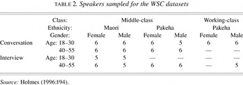
By contrast, the WSC data focused more on variation among middle-class New Zealanders by gender, age, and style (contrasting radio interviews with casual conversations). The sample analyzed contained only those cells of the age × gender × class × ethnicity × style crossproduct that could be filled by at least five speakers (Table 2); two of the WSC analyses were limited to Pakeha individuals (with 5 speakers added, for a total of 57 in those datasets).
Speakers sampled for the WSC datasets

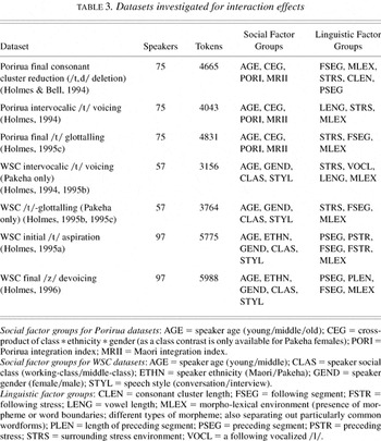
As shown in Table 3, the seven datasets cover five phonological variables: deletion of /t/ or /d/ in final consonant clusters; voicing or flapping of intervocalic /t/; glottal realization of syllable-final /t/; aspiration of syllable-initial /t/; and devoicing of word-final /z/. All of these datasets contain both linguistic and extralinguistic factor groups, allowing comparisons of interaction frequency between these sets; moreover, all consist of several thousand tokens, permitting the construction and testing of relatively detailed models.6
Freeman (1987:237) suggested that a model described by S parameters requires a number of tokens n > 10 (S + 1). This assumes complete independence of tokens, which, as already mentioned, may be false in linguistic data. Nevertheless, there is still a reasonable safety margin for constructing models with up to 100 factors in all of these datasets. Guy (1980:20) proposed a superficially similar empirical limit, for one factor group, of 10–30 tokens per factor per speaker, which L. Milroy (1987:135) linked to confidence intervals for cell proportions: but this does not directly scale up to cover a full multidimensional regression model.
Datasets investigated for interaction effects

Our original statistical analyses of these datasets in 1993–1995 did include a preliminary investigation of crosstabulations for possible interaction effects, some of which are footnoted in the original reports. No fuller description of linguistic interactions was possible at the time, however, because these reports were focused on interpreting variants' social distribution (extended and generalized across these variables in Holmes 1997a, 1997b) and on comparing NZE to other varieties of English (requiring linguistic descriptions to be closely compatible with previous studies). Moreover, the more systematic investigation procedure used here only became practical some years later.
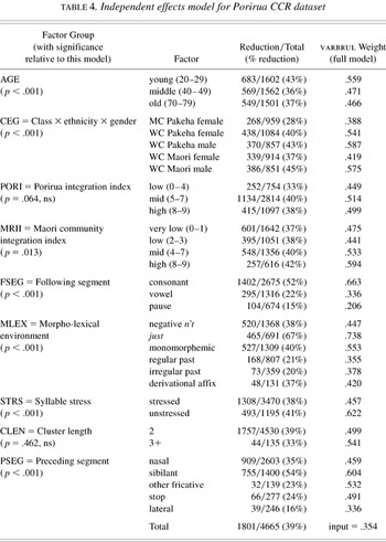
The Porirua consonant cluster reduction (CCR) dataset (Holmes & Bell, 1994) is singled out to illustrate the statistical and interpretative procedures employed. This dataset contains 4,665 tokens of syllable-final consonant clusters ending in /t/ or /d/, coded for the linguistic factors of morpholexical environment (distinguishing different types of morpheme and also separating out the most frequent lexical items); phonological segment following the consonant cluster; preceding phonological segment within the cluster; stress on the syllable containing the cluster; and cluster length. These linguistic factor groups were coded in accordance with accumulated analytical refinements from previous studies of the same variable, including Wolfram (1969), Fasold (1972), Bell (1977), Guy (1980), and Patrick (1991). Two small changes were made to the original coding for the current reanalysis: distinctions between different classes of following consonant were collapsed as all consonants had much the same main effect (Holmes & Bell, 1994:68);7
In retrospect, this may have been a mistake; some interaction might be expected between preceding and following consonants, reflecting differences in articulatory difficulty and/or potential for assimilation for the overall sequence. However, this does not affect the FSEG * STRS interaction presented.
Independent effects model for Porirua CCR dataset

Significance tests for interaction effects
Two different methods of testing variable-rule models for interaction effects were applied to every possible combination of two factor groups in each of the seven datasets.8
The present survey is limited to two-way interactions mostly for convenience (though also partly to avoid multicollinearity). Three-way or higher order interactions can in theory be added to a logistic regression model, but in practice all of the datasets considered here have far too many possible higher order interactions to test exhaustively using goldvarb (e.g., the nine factor groups of the Porirua CCR dataset allow 9 one-way tabulations, 36 two-way crosstabulations, 84 three-way interactions, 126 four-way interactions, and so on). Without some prior theoretical reason for including a specific interaction, three-way interactions can only be added indirectly, by first adding significant two-way interactions into the model and then conducting further significance tests against those.
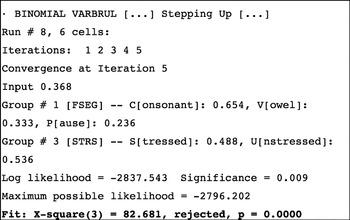
Figure 1 displays one test result for the Porirua CCR dataset. The model, assuming independence for the factor groups of following segment (FSEG) and syllable stress (STRS), is an extremely bad fit (p = .0000: i.e., p << .0001), indicating the presence of a significant interaction effect.

[Edited] goldvarb output for bottom-up model fit test of STRS * FSEG interaction in Porirua CCR dataset.
However, though a reasonable starting point, this approach can be somewhat unreliable, especially in more complex datasets. Each two-group model ignores the effects of any other factors that may be coded on the data, so this test can return a large number of false positives (and, less often, false negatives) where the cells of the crossproduct tested have significant associations with other influential factor groups.9
In one dataset for English impersonal subject relative pronoun choice, bottom-up tests identify 20 interactions as significant, of which all but three are subsequently found to be false positives (Sigley, 1997:294–301).
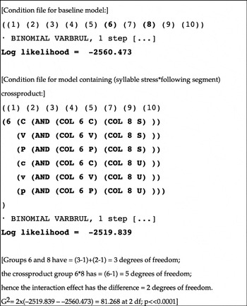
The second, more reliable, method, which may be called a “top-down” approach, uses goldvarb's estimate of the model likelihood (the probability that the dataset is in fact described by the model fitted to it) and asks whether the addition of some extra factor(s) makes the model a more likely fit to the data. The most complex independent effects model, containing all factor groups to be tested, is taken as a baseline model (Mb). A one-step variable rule regression run gives the log-likelihood for that model (ln Lb), and the degrees of freedom (the number of independently estimated parameter values) used in describing the model can be calculated as (the total number of factors) minus (the number of factor groups). The test compares Mb with a more complicated crossproduct model (Mc), constructed by replacing two of the original factor groups with a single factor group containing all possible combinations of their values: the difference between these models is exactly the interaction between those two factor groups. The same calculations are performed to obtain the new model's log-likelihood (ln Lc) and degrees of freedom. The test statistic, G2, is twice the difference in log-likelihood between the two models (= 2 * (ln Lc − ln Lb)) and can be compared to a chi-squared distribution at the difference in degrees of freedom between the two models. This is the same G2 test that goldvarb uses to add or subtract factor groups during a step-up/step-down regression run, as mentioned in Rousseau and Sankoff (1978a:65f); a more comprehensive description is provided in Paolillo (2002:85–92).
Figure 2 shows the condition files (and resulting log-likelihoods) for the Porirua CCR baseline model (Table 4) and for the model containing the STRS * FSEG crossproduct. There is a highly significant increase in model likelihood on including the interaction effect (G2(2df) = 81.268; p << .0001), which confirms the result of the bottom-up test.

[Edited] goldvarb output for top-down likelihood ratio test of STRS * FSEG interaction in Porirua CCR dataset.
Though the top-down test is more reliable, it is harder to carry out a large batch of such tests: fresh condition files and cell files are needed for every test, and goldvarb does not automatically calculate or evaluate the test statistic. It was also, until recently, too time-consuming to use systematically on complex datasets, though advances in processor speed have now removed that obstacle.10
Using goldvarb to construct just one model for a dataset of several thousand tokens with 15 factor groups took several days(!) on a Macintosh SE (ca. 1988), several hours on an LC3 (ca. 1992) and 30 minutes on a PowerMac (ca. 1996), but it takes less than a minute on a 500 MHz G4: thus the limiting step is now the process of coding the condition files. For this reason, the suggestion in Sigley (1997:254) that analysts could save time without sacrificing accuracy by performing the complete set of bottom-up tests first, and then using the top-down test just to check apparently significant test results, is now a little dated.
Choosing significance levels for multiple comparisons
For either test method, there is an additional problem in deciding what significance level to adopt. The conventional 5% level for an individual test means little when many tests are performed on the same dataset: in a group of more than 20 tests, we would expect at least one to reach the conventional significance level by chance. One common solution to this problem is the Bonferroni correction or Dunn's test (e.g., Stevens, 1986:6ff), which assumes the test results are independent and calculates a critical significance value such that the probability of at least one test of the set reaching significance is 5%. The Bonferroni equation for this limit on the “true” significance level (p*) from a set of N independent tests, given an observed p value = po, is given in (2):

thus, setting p* at 0.05, we require: po ≥ 1 − (1 − .05)(1/N) ≈ 0.05/N.
However, this limit may be too conservative if significant interaction effects are in fact found (as this also implies that tests are less likely to be independent). The compromise used here is the “sequentially rejective” Bonferroni procedure (Hochberg & Tamhane, 1987:58), which amounts to carrying out the standard Bonferroni correction but then ignoring the significant test results and repeating the calculation only for the remaining reduced set of apparently nonsignificant tests. This raises the critical p value, which may identify other tests as significant, thus necessitating further iterations until no new significant tests are identified. For example, suppose a set of ten significance tests return the p values in (3):

At the conventional level of p = .05, six tests (in boldface) are apparently significant, but the probability of at least one of the ten tests reaching that p value is unacceptably high: (1 − (1 − .05)10>) = .401. If we want the latter limit to be .05, then the critical value for a single test's observed p-value could be as low as po = (1 − (.95)1/10) = .0051, with only three test results (underscored) reaching statistical significance. The sequentially rejective procedure then calculates a new critical p value for the seven remaining nonsignificant tests: po,1 = (1 − (.95)1/7) = .0073. Two tests from the set have a p value below this revised value. A final iteration yields po,2 = (1 − (.95)1/5) = .0102, with no further test results being identified as significant; hence this is the final critical value, and five test results are significant at that level.
THE INCIDENCE OF INTERACTION EFFECTS: SIGNIFICANCE TEST RESULTS FOR TWO-WAY COMPARISONS
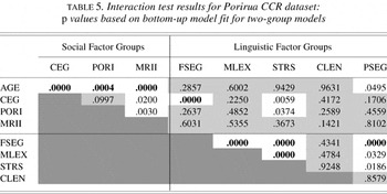
Table 5 shows the significance results for all the bottom-up tests applied to the Porirua CCR dataset. There are 36 pairs of factor groups to test, giving an initial critical p value of 1 − (.95)1/36 ≈ .05/36 = .0014; eight interactions are apparently significant, giving a final critical p value of 1 − (.95)1/(36-8) ≈ .05/28 = .0018, with no new significant tests. Tests significant at p = .0018 are shown in boldface, whereas tests nonsignificant at the conventional 5% level are shaded out. The interactions identified as apparently significant by this method are the three interactions between AGE and the other social factor groups (AGE * CEG, AGE * PORI, AGE * MRII); an interaction between following segment and class/ethnicity/gender; and four interactions between linguistic factor groups, of which three involve the following segment (FSEG * MLEX, FSEG * STRS, FSEG * PSEG, and MLEX * STRS).
Interaction test results for Porirua CCR dataset: p values based on bottom-up model fit for two-group models

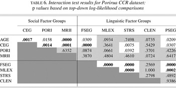
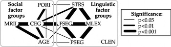
The top-down log-likelihood test results for the same dataset are presented in Table 6. Ten tests are significant at a final Bonferroni-corrected critical value of .0020, and these include seven of those identified as significant in Table 5. The differences are that the AGE * PORI interaction does not quite reach the required significance level, whereas the CEG * PORI, CEG * MRII, and MLEX * PSEG interactions do. The pattern of significance results for apparent interaction effects in a dataset may be most briefly summarized by plotting the relative significance of the interactions on a network diagram directly analogous to that used for displaying interactions between individuals (L. Milroy, 1980), as in Figure 3. In this case, the plot shows a set of strong interactions among the social groups, centered on CEG; strong interactions among the linguistic factor groups MLEX, PSEG, FSEG, and STRS; and, apart from FSEG * CEG, generally weaker apparent interactions between the two sets of factor groups. All factor groups except consonant cluster length are involved in at least one apparently significant interaction. Though the two tests give broadly similar results on this dataset, such high consistency between the two test methods is not guaranteed. On more complex datasets, most of the apparently significant results from the bottom-up test may be false positives resulting from associations with other coded factor groups. For this reason, I cite only the top-down test results.
Interaction test results for Porirua CCR dataset: p values based on top-down log-likelihood comparisons


Distribution of apparently significant interaction effects across factor groups for the Porirua CCR dataset.
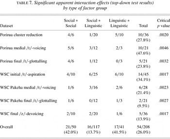
Applying the top-down test to all pairs of factor groups within each of the seven datasets provides the distribution of test significance shown in Table 7. The most notable feature is that over the seven datasets as a whole, more than a quarter (54 of 208, or 26%) of the possible pairwise crossproducts contain significant apparent interaction effects. If some term(s) from each significant crossproduct were included as a new factor group, this would almost double the total number of factor groups. This demonstrates that, for these variables, even a full presentation of all coded main effects, such as Table 4, is still incomplete and may leave many other potentially important explanatory factors as yet unidentified. Moreover, this is true even for the variables of /t,d/-deletion and intervocalic /t/-voicing, where the coding categories used were informed by decades of previous study. The proportion of significant interaction effects differs considerably between datasets, ranging from roughly 10% (WSC /t/-glottalling) to roughly 50% (Porirua /t/-voicing); this proportion could be used as an index of how much is missing from descriptions of these variables, which assume complete independence of main effects.
Significant apparent interaction effects (top-down test results) by type of factor group

The apparently significant interaction effects are divided by class of factor group as follows. First, extralinguistic factor effects frequently interact amongst themselves, as expected from the variationist literature to date, with interaction effects reaching significance in 42% of possible cases. Rather less expectedly, however, significant pairwise interactions between linguistic factor effects are just as common (at 41.5%). Thus both social and linguistic factors show frequent interaction effects, and with about the same frequency in this data, in striking opposition to the description presented by Fasold (1991). Finally, significant interactions between extralinguistic and linguistic factors, while less likely (at 13% of pairwise tests), are still not so rare as to be negligible, indicating that there may be some statistical differences between different social groups in the linguistic system governing these variables. This result implies that it may not generally be possible to consider linguistic and extralinguistic factor groups as having separate effects; they should at least be combined in an initial analysis to check for interactions.
INTERPRETING AND INTEGRATING INTERACTION EFFECTS
Having established that interaction effects are important in a statistical sense, it remains to demonstrate their practical and theoretical importance for improving models of variation. This requires that we consider the tightly linked issues of how to interpret interaction effects and how to integrate them into a model.
The statistical tests presented here have the main function of identifying potentially interesting factor crossproducts for more detailed investigation. Taking each of these factor crossproducts in order of decreasing significance (or else in sets sharing the same factor groups), we need to identify some specific pattern of interaction and attempt an interpretation before we can decide how best to incorporate the interaction within a model. Simply adding an unmodified crossproduct factor group to all the original factor groups is not recommended: this usually introduces an unacceptable level of redundancy, as the crossproduct group contains within it all the information from its component factor groups, giving rise to multicollinearity (see note 3). Choosing exactly which new distinctions to add is at least partly a statistical question; but there are then several largely equivalent choices as to where or how to add them, and that decision is often more a matter of interpretation.
The first step is to identify patterns unpredictable from main effects. Several different approaches are possible. Visual inspection of crosstabulations is a logical starting point for analysts seeking to ground their descriptions in observed reality, but it is one with important limitations, such as: not controlling for associations; and presenting differences which combine main and interaction effects. The second of these problems, isolating interaction effects from main effects in a crosstabulation, may be solved by calculating the residuals (the differences between actual cell proportions and those predicted by the two-group independent-effects model as used in the bottom-up test; residuals may also be scaled to standard normal variates as an approximate indicator of significance).11
This is, in essence, the bottom-up chi-squared test presented in a different form (the theoretical chi-squared distribution at 1df is in fact z2).
By contrast, splitting an entire model over a factor group (though it may end up as the only way of modelling datasets with many higher-order interactions) offers much less controlled comparisons of factor effects because the effects of all other factor groups are calculated separately for each submodel (Paolillo, 2002:91).
As an illustration of some of these procedures, I now return to the effects of syllable stress and following segment on /t,d/-deletion in the Porirua CCR dataset.
Inspecting a crosstabulation
In their initial description of the CCR dataset, Holmes & Bell (1994) identified a highly significant main effect from following segment (with reduction favored by following consonants and disfavored by a following pause) and a “small but significant” (p. 71) effect from syllable stress (with reduction slightly favored in unstressed syllables). This description is consistent with the main effect factor weights given for these groups in Table 4. Moreover, these effects make theoretical sense: a following consonant increases articulatory difficulty, so is expected to favor cluster reduction, while tokens that are unstressed may be expected to be less fully articulated in general (see also Guy, 1980:8).
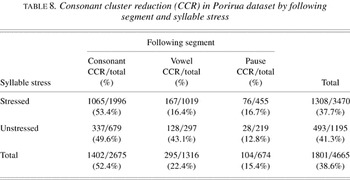
However, these main effects do not tell the whole story. The crosstabulation of reduction frequencies in Table 8 indicates that the expected stress effect occurs only in tokens immediately followed by a vowel and, in this subenvironment, is far from “small”. The observed frequency of reduction in unstressed syllables (43.1%) is more than twice that in stressed syllables (16.4%). When either a consonant or a pause follows the cluster, there instead seems to be a weak tendency for cluster reduction to be favored by stress. But this apparent difference is quantitatively extremely small (reduction is about 4% more likely in both environments) and theoretically unexpected, so it may result from associations with other factors, or from other interaction effects. For example, the effect of a following consonant might be stronger in stressed syllables or weaker in unstressed syllables, and this interaction could outweigh the overall stress effect. Comparing the table rows also shows an apparent effect dependence whereby vowel and pause effects are distinguished only after an unstressed syllable. In either case, the frequency of cluster reduction in unstressed syllables followed by a vowel is clearly not predictable from the average effects for unstressed syllables or for a following vowel, but the interpretation of other cells is less clear.
Consonant cluster reduction (CCR) in Porirua dataset by following segment and syllable stress

Isolating the interaction effects
In more complex crosstabulations, it can be even harder to locate important interaction effects by simple inspection. One step towards isolating and displaying interaction effects separately from main effects is to calculate the residuals, or the differences between the actual cell frequencies and those estimated by the independent-effects model used in the bottom-up test (see Figure 1). From the logistic equation in (1), the modelled cell percentage

in a two-group model is

where

= the “input probability”, and

are the parameter values reported for the two factors actually present in the cell. The estimated cell percentages for the stress * following segment crossproduct can be calculated from the factor weights shown in Figure 1 (where the model has an input weight of .368). For example, the SC cell, for a stressed syllable (model weight = .488) followed by a consonant (model weight = .654), has a modelled cell percentage given by:

The residual is then just

, = (53.4% − 51.2%) = +2.2% for this cell.
Residuals may also be converted into standard normal (z) variates,

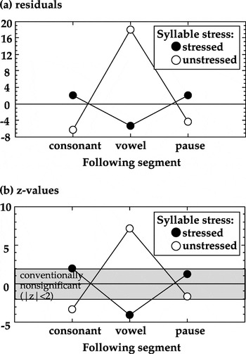
where n = the number of tokens in the cell, and these may be used as an approximate measure of which cells contribute most to the significance of an interaction effect (a z variate with an absolute value of 2 corresponds roughly to the conventional 5% significance level). Figure 4 displays the residuals, and the derived z values, for a comparison of actual and modelled proportions of cluster reduction in the cells of Table 8. The plots in Figure 4 confirm the foregoing description based on cell percentages, in that the single largest difference from the independent effects model is the higher than expected cluster reduction in stressed tokens followed by a vowel (with a z value of 7.134, p << .0001), while other residuals are relatively small (and represent nonsignificant differences for following pause).

Residuals (actual − model% CCR) and z values for the crosstabulation of syllabic stress and following segment.
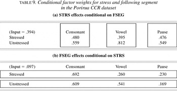
However, a description of factor effects in different environments is more accurately based on factor weights than on observed cell percentages, as the latter may be skewed by associations with other coded factor groups. A controlled comparison of effects is most easily performed by modelling conditional effects for each of the two factor groups. For this case, this involves constructing two models, the first partitioning STRS by FSEG within a single model (including three separate stress groups, each modelling stress effects independently for a different FSEG environment, but not including any explicit FSEG group), and the second partitioning FSEG by STRS (i.e., using two FSEG groups to model following segment effects independently in each stress environment, but not including any explicit STRS group) within an otherwise identical model. Each of these two models is equivalent to the model containing the full STRS * FSEG crossproduct, except for choosing different reference points for describing different parts of the crossproduct group, resulting in vastly different input weights. Weights for all other factor groups are identical (and the models have the same log-likelihood, within the limits of rounding error). The factor weights reported just for these groups from these two models are given in Table 9. (Because these are equivalent perspectives on the data, it is important to attempt an interpretation for both sets of conditional weights.)
Conditional factor weights for stress and following segment in the Porirua CCR dataset

The conditional stress effect values (Table 9a) confirm a much stronger effect for unstressed syllables before a vowel (weight = .812) than elsewhere. This comparison also immediately shows that the effects of stress are essentially the same before consonants as before pauses and are in the expected direction within each environment (unstressed syllables consistently favor cluster reduction), in contrast to the apparent effect reversal for stress before a consonant seen in the raw figures of Table 8. Meanwhile, the conditional effects of following segment (Table 9b) confirm that the effects of following vowel and pause are essentially the same on stressed tokens (.260 and .230, respectively), but must be distinguished for unstressed tokens, and that the effect of a following consonant is stronger on stressed tokens (weight = .692, compared to .609 for unstressed tokens).
Interpreting interaction effects
Because interaction effects are by definition limited to a subset of the data, they do not permit easy generalizations and are accordingly more difficult to interpret than main effects. This is a particular problem because there are at least three conceptually rather different causes for apparent interaction effects, each suggesting a different solution, and any real example may require some combination of all of these.
First, there could in fact be a causal interaction effect, in which the effects of some factor(s) on one group directly exaggerate, cancel, or reverse the effects of some factor(s) on another group. Such effects may be causally interpretable in terms of the proposed explanations for the main effects of the factor groups, in which case the factors included, and their interpretations, may need no other changes. Several different modelling solutions are possible. If only one cell is involved, this can be modelled using a dummy interaction factor group contrasting that cell with everything else. In more extreme cases, where an entire factor group makes a difference only in combination with certain other factor(s) and is otherwise irrelevant, we may need to split the factor group or even split the model, so that its effects are included only for the relevant subset or modelled separately for different subsets. If a large number of different interactions are identified, it may be better to consider the two factor groups as components of one underlying causal dimension and thus adopt (some simplified version of) the crossproduct in our model; or it may be possible to recombine the crossproduct cells to more directly reflect some set of simpler explanatory dimensions.
Second, apparent interaction effects could indicate that the values or meanings of the classification labels used are not constant but rather contingent on other factors (as with the example of gender and class definitions). This requires re-evaluating the explanatory value and descriptive unity of the original factors, most likely with the eventual result of adding some distinction(s) from the crossproduct into one of the original factor groups.
Third, an apparent interaction effect could indicate the presence of some significant uncoded factor unevenly distributed across the cells of the crosstabulation. This requires that analysts identify the cells that show the most unpredictable behavior and re-examine the tokens representing those cells to check whether they share some factor(s) as yet unidentified; any such factors found should then be coded and included in some new factor group(s), in addition to the original groups. (There are, however, limits to how far this procedure can be applied in the present study without going back to the original audio data.)
In the case of the STRS * FSEG interaction, it is possible to explain the nonlinear combination of effects from stress and following consonant directly in terms of the explanations given for the effect of each factor. If following consonants favor reduction because they increase articulatory complexity, it is not surprising that this effect should be magnified in a stressed environment where articulation is generally more precise.
The increased contrast between stress effects before a following vowel is a little less predictable from the component factors alone, but may be explained by the presence of additional uncoded factors. One hypothesis is that the following vowel environment may include a high proportion of reduced (and unstressed) realizations of function words such as articles/determiners (a, his, her), auxiliaries (is, are, am, have, had, will, would), conjunctions (and, or), object pronouns (her, him, it), and the most frequent prepositions (in, of, at). In such cases, we would predict that the effect of an unstressed environment in favoring reduction would be greatly magnified, not just through the continued reduction of stress, but also because (to the extent that New Zealand English is stress-timed) a longer sequence of unstressed syllables would lead to a more rapid local rate of speech, exaggerating any tendency for articulatory reduction (see Guy, 1980:9, who suggested that speech rate has a potentially important influence on /t/-deletion, but had no direct way of measuring it). This hypothesis should be tested by going back to the original audio data and adding factor groups for following stress and/or grammatical status of any immediately following word. Pending such coding refinements, it should be noted that there is some highly relevant social variation within New Zealand English, with Maori showing a significantly stronger tendency for syllable-timing as measured by full pronunciation of function words (Holmes & Ainsworth, 1996). This explanation of the FSEG * STRS interaction may thus also account for the apparent CEG * FSEG (p < .0001) and CEG * STRS (p = .0075) interactions observed for this dataset (though again, confirmation will only be possible after additional coding of the raw data).13
Guy's (1980) observed differences for New York and Philadelphia speech in the effect of a following pause may ultimately have a similar explanation in terms of more general dialectal differences in speech rate and stress pattern rather than from pause per se.
Adding interaction effects to a model
The STRS * FSEG interaction effects have now been given a plausible linguistic interpretation and so may be explicitly added into the Porirua CCR model. However, this should not be done by adding the unmodified crossproduct group (which, first, loses any explanatory generalizations possible for the original groups, and second, would make it difficult if not impossible to investigate other interactions involving the STRS and FSEG groups). Whether or not to use a simpler model than that containing the full crossproduct group can be assessed by comparing model log-likelihoods (again, using a G2 test at the difference in model degrees of freedom); the aim of such a comparison is to find a model that is simpler (using fewer degrees of freedom) without being significantly less likely than the crossproduct model.
The analysis of conditional weights suggests it would be desirable for a coding solution to maintain distinctions between the UV, UC, and SC environments, while collapsing some of the distinctions between UP, SP, and SV. Even within these constraints, however, there are still several possible ways that these significant (and interpreted) cell effects could be added to an overall model of variation. The condition files for three such models are presented in Figure 5, together with their log-likelihoods, and the results of G2 tests against the model containing the full STRS * FSEG crossproduct. The contrasting approaches they represent are as follows:

Condition files and log-likelihoods for alternative models incorporating STRS * FSEG interaction effects.
(i). Keep the original factor groups, but add an extra dummy factor group specifically for the UV environment
This uses four degrees of freedom to describe the variation due to FSEG and STRS, so is a slightly simpler model than the full STRS * FSEG crosstabulation (using 5df). As it happens, the log-likelihood for this model is almost the same as that for the model including the STRS * FSEG crossproduct (G2(1df) = .002, p = .9643). (However, attempts to add further dummy groups for the SC and UC environments resulted in multicollinearity.)
(ii). Use the crossproduct group, but look for ways to simplify it
The guidelines just given suggest that the crossproduct could be optimally simplified by combining UP, SP, and SV as one category. This simplification does not significantly reduce model likelihood (G2(2df) = 1.650, p = .4382), so should be considered a better solution than the full-crossproduct model.
(iii). Recombine the crossproduct cells in a different, theoretically motivated way
The working interpretation for the cell effects makes reference to two dimensions (articulatory complexity, and the local rate of speech as estimated indirectly from information about stress patterns and pauses), so it is natural to attempt to recombine the crossproduct cells to capture these dimensions separately. Articulatory complexity can be simply captured in terms of whether or not there is a following consonant. Local rate of speech is a little more arbitrary and can only be estimated very approximately without direct reference to the as yet uncoded factor group of following stress. However, combining the assumptions that a following pause may be more typical of slow speech (P ≤ C,V), that following vowels are more likely to correspond to unstressed function words and thus faster speech (C < V), and that stressed syllables are more typical of slow speech (S < U) results in the partial ordering of cells in (6), so that the cells can be recombined into three groups as Slow = {SP,SC}; Medium = {SV,UP,UC}; and Fast = {UV}. The crosstabulation of these two factor groups maintains all of the necessary cell distinctions from the original crossproduct, while collapsing SV and UP.

Again, the model resulting from this reclassification is simpler than the full crossproduct without leading to a significant decrease in likelihood (G2(2df) = .804, p = .669). Hence model (iii) almost completely accounts for the observed FSEG * STRS interaction effects, but without including any explicit interaction term.
Thus there are three possible models for the STRS * FSEG effects in this data, all of which are preferable to the full crossproduct and highly preferable to the original independent-effects model. Of the three, model (i) is the most likely, but also uses one more degree of freedom. No strong statistical reasons exist for choosing one model over the others; they may be considered almost exactly equivalent ways of looking at this variation (demonstrating amongst other things that interaction effects and main effects may be interchangeable).
The final choice of model thus relies mostly on whether an analyst prefers (i) to keep the original (fairly easily observed, and thus replicable) descriptive dimensions, with an additional factor group for their interaction; (ii) to combine the two factor groups as representing one descriptive dimension; or (iii) to reinterpret the data in terms of independent effects from a more directly explanatory, but also more abstract and less directly observable, set of dimensions. In this case, the observable correlates (original factor groups) of the abstract dimension(s) (final reinterpreted groups) may well differ between social groups, even if they use the same rule at the more abstract level, and this will create apparent interaction effects as analysts describing data have no choice but to use consistent criteria for coded distinctions. These are, of course, exactly the same choices and issues that analysts are accustomed to dealing with when interpreting social categories; it is perhaps worth reminding ourselves that they apply equally to linguistic categories, as well.
CONCLUSION: THE IMPORTANCE OF INTERACTION EFFECTS
The survey of interaction effect frequency conducted here indicates that highly significant interaction effects are rather more common in linguistic data than has been previously realized, and occur as often between linguistic factors as between social factors. Thus there is a general sense that any models of linguistic variation that include only main effects from initially observed correlates must be regarded as incomplete accounts, which may fail to capture a large part of the variation. As a result, it is absolutely imperative that the presence of interaction effects be systematically tested for, and that the overall results of these tests be reported.
For the researcher, a systematic study of interaction effects can indicate the existence of unencoded effects and so indicate how inclusive the initial model actually is; moreover, the significance of individual interaction effects can be used to indicate the relative importance of unencoded effects compared to the coded factor groups. (All of the interaction effects counted as significant in this study had much lower p values than the conventional 5% level used by goldvarb in identifying significant main effects.) Conducting the full battery of tests identifies interesting crossproducts for investigation and thus speeds up and systematizes the identification and interpretation of the most useful effects.
The wider importance of interaction effects for the investigation of (socio)linguistic variation becomes apparent, however, when the attempt is made to interpret them. The present case study of the combined effects of stress and following segment on /t,d/-deletion in final consonant clusters demonstrates that interaction effects are explicanda just as important as main effects, and that the two types of effect can represent largely equivalent ways of looking at the same data, depending on how analysts define their descriptive dimensions. The results of detailed investigations of interactions can suggest new factors not initially encoded and/or new interpretations for the factors that are encoded. More generally and most importantly, whereas use of main-effects models is essentially confirmatory (only telling the analyst whether or not the data is consistent with some already-formulated hypothesis), identification and analysis of interaction effects generate further hypotheses and thus allow a way forward from the initial model. If statistical modelling is to be used as a discovery procedure, rather than as an end in itself, then it is in the interaction effects that the most new discoveries lie.
References
REFERENCES
Bell, Allan.
(1977).
The language of radio news in Auckland: A sociolinguistic study of
style, audience and sub-editing variation.
Doctoral dissertation,
University of Auckland.
Bickerton, Derek.
(1971).
Inherent variability and variable rules.
Foundations of Language
7:457–492.Google Scholar
Cedergren, Henrietta J.
(1973).
On the nature of variable constraints. In
Charles-James N. Bailey &
Roger W. Shuy (eds.),
New ways of analyzing variation in English.
Washington, DC:
Georgetown University Press.
13–22.
Eckert, Penelope.
(1989).
The whole woman: Sex and gender differences in variation.
Language Variation and Change
1:245–267.Google Scholar
Fasold, Ralph W.
(1972).
Tense marking in Black English: A linguistic and social analysis.
Arlington, VA:
Center for Applied Linguistics.
Freeman, Daniel H, Jr.
(1987).
Applied categorical data analysis.
New York:
Marcel Dekker.
Godfrey, Elizabeth, &
Tagliamonte, Sali.
(1999).
Another piece for the verbal -s story: Evidence from Devon
in southwest England.
Language Variation and Change
11:87–121.Google Scholar
Gordon, Elizabeth.
(1997).
Sex, speech and stereotypes: Why women use prestige speech forms
more than men.
Language in Society
26:47–63.Google Scholar
Guy, Gregory.
(1980).
Variation in the group and the individual: The case of final stop
deletion. In
William Labov (ed.),
Locating language in time and space.
New York:
Academic.
1–36.
Hochberg, Josef, &
Tamhane, Ajit C.
(1987).
Multiple comparison procedures.
New York:
Wiley.
Holmes, Janet.
(1994).
New Zealand flappers: An analysis of T voicing in New Zealand
English.
English World-wide
15:195–224.Google Scholar
Holmes, Janet.
(1995a).
Time for /t/: Initial /t/ in New Zealand English.
Australian Journal of Linguistics
15:127–156.Google Scholar
Holmes, Janet.
(1995b).
Two for /t/: flapping and glottal stops in New Zealand
English.
Te Reo
38:53–72.Google Scholar
Holmes, Janet.
(1995c).
Glottal stops in New Zealand English: An analysis of variants of
word-final /t/.
Linguistics
33:433–463.Google Scholar
Holmes, Janet.
(1996).
Losing voice: Is final /z/ devoicing a feature of Maori
English?
World Englishes
15:193–205.Google Scholar
Holmes, Janet.
(1997a).
Maori and Pakeha English: Some New Zealand social dialect data.
Language in Society
27:65–101.Google Scholar
Holmes, Janet.
(1997b).
Setting new standards: Sound changes and gender in New Zealand
English.
English World-wide
18:107–142.Google Scholar
Holmes, Janet, &
Ainsworth, Helen.
(1996).
Syllable-timing and Maori English.
Te Reo
39:75–84.Google Scholar
Holmes, Janet, &
Bell, Allan.
(1994).
Consonant cluster reduction in New Zealand English.
Wellington Working Papers in Linguistics
6:56–82.Google Scholar
Holmes, Janet,
Bell, Allan, &
Boyce, Mary.
(1991).
Variation and change in New Zealand English: A social dialect
investigation.
Wellington:
Department of Linguistics, Victoria University of Wellington.
Holmes, Janet,
Vine, Bernadette, &
Johnson, Gary.
(1998).
Guide to the Wellington Corpus of spoken New Zealand English.
Wellington:
Victoria University of Wellington.
Kikai, Akio,
Schleppegrell, Mary, &
Tagliamonte, Sali.
(1987).
The influence of syntactic position on relativisation strategies.
In
Keith Denning,
Sharon Inkelas,
Faye McNair-Knox, &
John Rickford (eds.),
Variation in language: NWAV-XV at Stanford.
Stanford:
Department of Linguistics, Stanford University.
266–277.
Milroy, James.
(1992).
Language variation and change.
Oxford:
Blackwell.
Milroy, Lesley.
(1980).
Language and social networks.
Oxford:
Blackwell.
Milroy, Lesley.
(1987).
Observing and analysing natural language: A critical account of
sociolinguistic method.
Oxford:
Blackwell.
Mougeon, Raymond, &
Nadasdi, Terry.
(1998).
Sociolinguistic discontinuity in minority language communities.
Language
74:40–55.Google Scholar
Paolillo, John.
(2002).
Analyzing linguistic variation: Statistical models and methods.
Stanford:
CSLI Publications.
Patrick, Peter L.
(1991).
Creoles at the intersection of variable processes: -t,d deletion
and past marking in the Jamaican mesolect.
Language Variation and Change
3:171–189.Google Scholar
Rousseau, Pascale.
(1989).
A versatile program for the analysis of sociolinguistic data. In
Ralph Fasold &
Deborah Schiffrin (eds.),
Language change and variation.
Amsterdam:
Benjamins.
395–409.
Rousseau, Pascale, &
Sankoff, David.
(1978a).
Advances in variable rule methodology. In
David Sankoff (ed.),
Linguistic variation: Models and methods.
New York:
Academic.
57–69.
Rousseau, Pascale, &
Sankoff, David.
(1978b).
A solution to the problem of grouping speakers. In
David Sankoff (ed.),
Linguistic variation: Models and methods.
New York:
Academic.
97–117.
Sankoff, David.
(1988).
Variable rules. In
U. Ammon,
N. Dittmar, &
K. Matthier (eds.),
Sociolinguistics: An international handbook of the science of
language and society.
Berlin:
de Gruyter.
140–61.
Sankoff, David, &
Laberge, Suzanne.
(1978).
Statistical dependencies among successive occurrences of a
variable in discourse. In
David Sankoff (ed.),
Linguistic variation: Models and methods.
New York:
Academic.
119–126.
Scherre, Maria Marta Pereira, &
Naro, Anthony J.
(1991).
Marking in discourse: “Birds of a feather.”
Language Variation and Change
3:23–33.Google Scholar
Scherre, Maria Marta Pereira, &
Naro, Anthony J.
(1992).
The serial effect on internal and external variables.
Language Variation and Change
4:1–13.Google Scholar
Sigley, Robert.
(1997).
Choosing your relatives: Relative clauses in New Zealand English.
Doctoral dissertation,
Victoria University of Wellington.
Stevens, James.
(1986).
Applied multivariate statistics for the social sciences.
Hillsdale, NJ:
Erlbaum.
Wolfram, Walt.
(1969).
A sociolinguistic description of Detroit Negro speech.
Washington, DC:
Center for Applied Linguistics.
Woods, Anthony,
Fletcher, Paul, &
Hughes, Arthur.
(1986).
Statistics in language studies.
Cambridge:
Cambridge University Press.

Porirua dialect survey interview sampling frame
Speakers sampled for the WSC datasets
Datasets investigated for interaction effects
Independent effects model for Porirua CCR dataset
[Edited] goldvarb output for bottom-up model fit test of STRS * FSEG interaction in Porirua CCR dataset.
[Edited] goldvarb output for top-down likelihood ratio test of STRS * FSEG interaction in Porirua CCR dataset.
Interaction test results for Porirua CCR dataset: p values based on bottom-up model fit for two-group models
Interaction test results for Porirua CCR dataset: p values based on top-down log-likelihood comparisons
Distribution of apparently significant interaction effects across factor groups for the Porirua CCR dataset.
Significant apparent interaction effects (top-down test results) by type of factor group
Consonant cluster reduction (CCR) in Porirua dataset by following segment and syllable stress
Residuals (actual − model% CCR) and z values for the crosstabulation of syllabic stress and following segment.
Conditional factor weights for stress and following segment in the Porirua CCR dataset
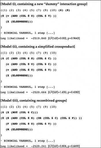
Condition files and log-likelihoods for alternative models incorporating STRS * FSEG interaction effects.
 You have
Access
- 18
- Cited by