2. Theory

Although in special cases weakly nonlinear theory can be used to predict the evolution of a moderately large-amplitude internal solitary wave as it interacts with topography (Maderich et al. Reference Maderich, Talipova, Grimshaw, Pelinovsky, Choi, Brovchenko, Terletska and Kim2009, Reference Maderich, Talipova, Grimshaw, Terletska, Brovchenko, Pelinovsky and Choi2010), in general it is not possible to derive an analytic model for the approach and interaction of an internal solitary wave with submerged topography. Nonetheless, by examining the stability of shallow-water disturbances in a two-layer fluid, we can gain insight into its evolution and, in particular, the potential for breakdown due to mixing. In this approach, we consider a solitary wave of depression situated initially over topography so deep or so flat that the ambient can be approximated as having uniform depth. In the spirit of the Wentzel–Kramers–Brillouin (WKB) approximation, if the topography rises slowly compared to the horizontal extent of the wave, the wave is expected to evolve as if the underlying topography is locally flat. Thus we assess the stability of the wave with respect to its amplitude $A_{sw}$ , the (constant) upper-layer depth $H_{1}$ and the lower-layer depth $H_{2}$ , which is smaller when the wave is situated over a hill.

In considering the stability of the wave as it depends upon its relative amplitude, we suppose the ambient is a two-layer fluid of finite uniform depth, $H$ . In a stationary ambient, the upper layer has depth $H_{1}$ and density ${\it\rho}_{1}$ while the lower layer has depth $H_{2}$ and density ${\it\rho}_{2}$ . Arbitrarily we suppose that $H_{1}<H_{2}$ so that solitary waves are manifest as waves of depression, with the interface displaced downwards by ${\it\eta}(x,t)$ , taken to be positive. We also allow for the free surface to be displaced by ${\it\eta}_{0}(x,t)$ , which is taken to be positive if upwards. Thus in the presence of a wave, the upper layer has depth $h_{1}(x,t)=H_{1}+{\it\eta}+{\it\eta}_{0}$ and the lower layer has depth $h_{2}=H_{2}-{\it\eta}$ .

For shallow hydrostatic disturbances, momentum and mass must be conserved in each layer, so that

Here $u_{1}(x,t)$ and $u_{2}(x,t)$ are the horizontal velocities in the upper and lower layers, respectively. Consistent with the shallow-water assumption, the flows are independent of depth $z$ . With the understanding that $\Vert {\it\eta}_{0}\Vert$ is small compared to the layer depths and $\Vert {\it\eta}\Vert$ , and assuming that there is no flow in the absence of waves, we also have that

Following Long (Reference Long1956), we reduce (2.1)–(2.3) to two equations in $u_{1}$ and $h_{1}$ alone. These are scaled with respect to $H$ and the characteristic speed $c_{0}\equiv (g^{\prime }H)^{1/2}$ , in which $g^{\prime }=g({\it\rho}_{2}-{\it\rho}_{1})/{\it\rho}_{0}$ is the reduced gravity and ${\it\rho}_{0}$ is the characteristic density. Thus we define the non-dimensional functions $u\equiv u_{1}/c_{0}$ and $h=h_{1}/H$ and the scaled space and time variables ${\it\chi}=x/H$ and ${\it\tau}=c_{0}t/H$ . The resulting coupled pair of nonlinear equations are

Seeking solutions for unidirectional disturbances, the equations can be reduced further to one equation in one unknown using the method of characteristics. This can be done explicitly or using the transformation $a\equiv 1-2h$ and $b=u/(1-h)$ , which yields the appealing symmetric pair of equations $a_{{\it\tau}}+(b(a^{2}-1)/2)_{x}=0$ and $b_{{\it\tau}}+(a(b^{2}-1)/2)_{x}=0$ , upon which analyses can be more simply performed (Chumakova et al. Reference Chumakova, Menzaque, Milewski, Rosales, Tabak and Turner2009). The (scaled) characteristic speeds are

Whereas for a one-layer fluid the speeds are strictly real-valued, here we find that the speeds are real-valued (i.e. the system is hyperbolic) only if $\mathit{Ri}\equiv [(1\!-\!h)/u]^{2}\geqslant 1$ , a criterion written in terms of a bulk Richardson number because in dimensional units $\mathit{Ri}=g^{\prime }H/(u_{1}-u_{2})^{2}$ (Milewski et al. Reference Milewski, Tabak, Turner, Rosales and Menzaque2004; Chumakova et al. Reference Chumakova, Menzaque, Milewski, Rosales, Tabak and Turner2009). In terms of energetics, $\mathit{Ri}$ represents the potential energy gain due to mixing divided by the kinetic energy loss. If $\mathit{Ri}<1$ , the flow is sufficiently energetic that it could completely mix the two layers (Milewski et al. Reference Milewski, Tabak, Turner, Rosales and Menzaque2004).

The Riemann invariants of the two-layer shallow-water system are

In particular, for rightward-propagating disturbances satisfying $u=0$ if $h=\widetilde{H_{1}}\equiv H_{1}/H$ , we have from $r_{-}=\sin ^{-1}(1-2\widetilde{H_{1}})$ that

Thus we can write the stability criterion, $\mathit{Ri}\geqslant 1$ , in terms of $h$ alone. In dimensional units, this sets a limit, $A_{c}$ , on the amplitude of an internal solitary wave:

Alternatively, the critical condition can be written in terms of the maximum deepening of the upper layer such that $H_{1}+A_{sw}\leqslant H/2+\sqrt{H_{1}H_{2}}$ , in which $H=H_{1}+H_{2}$ is the total ambient depth. Because the geometric mean is always less than the arithmetic mean of $H_{1}$ and $H_{2}$ , the right-hand side of this inequality is always less than the total fluid depth.

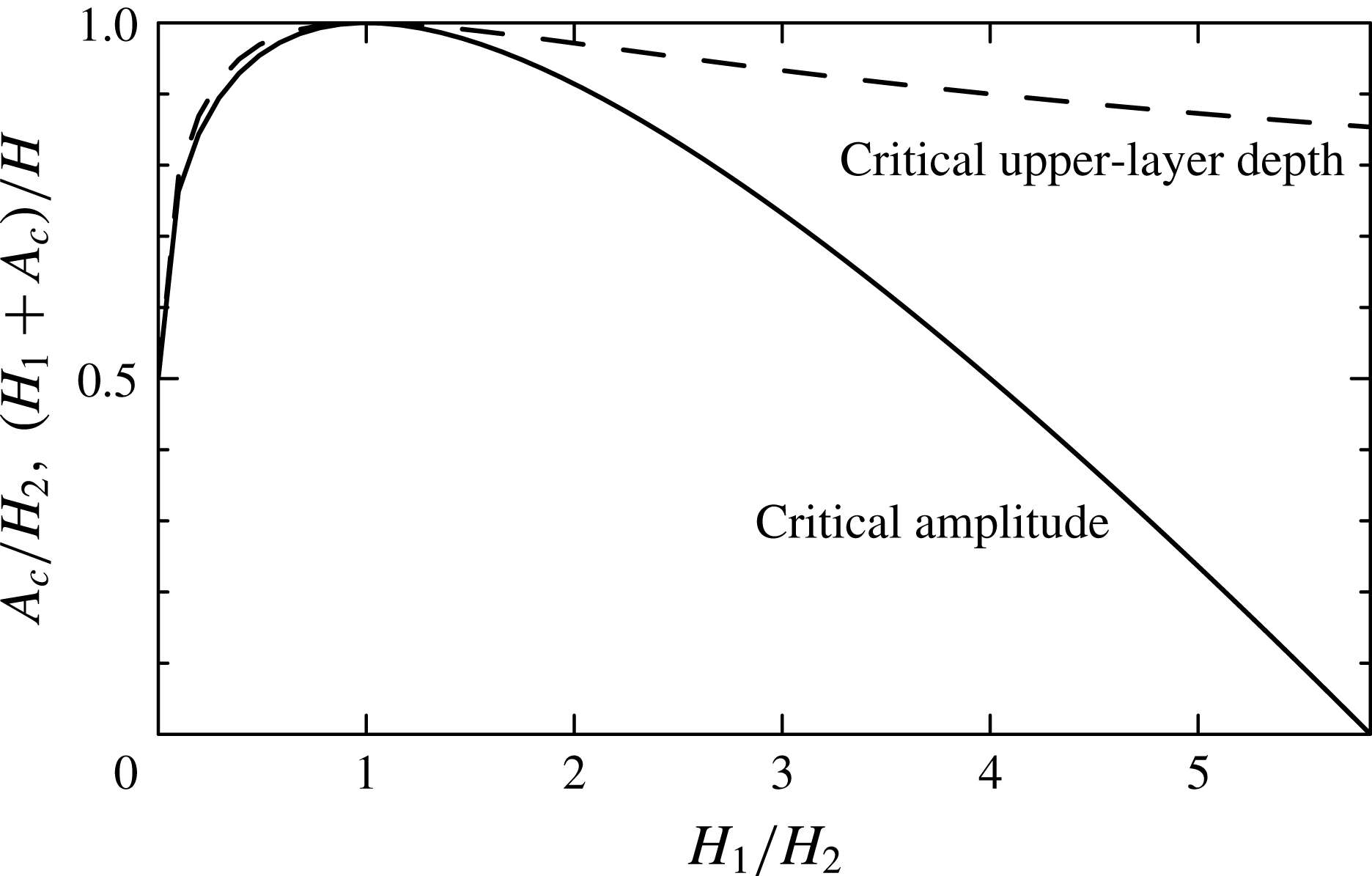
The predicted critical value is plotted in figure 1. In the limit of a relatively shallow upper layer ( $H_{1}/H_{2}\rightarrow 0$ ), the prediction gives the usual expression for the limiting amplitude: $H_{1}+A_{sw}\lesssim (H_{1}+H_{2})/2~\Rightarrow ~A_{sw}\leqslant H_{2}/2$ . If $H_{1}=H_{2}$ , then the amplitude of the wave can be almost as large as the lower-layer depth without having sufficient kinetic energy to uniformly mix the fluid column. However, as the lower layer becomes relatively more shallow, the critical amplitude for stability decreases up to the limit $H_{1}/H_{2}=3+2\sqrt{2}$ , beyond which any downward-displaced disturbance has sufficient kinetic energy to mix the ambient.

Figure 1.

Predicted critical amplitude, $A_{c}$ , of an internal solitary wave of depression in a shallow-water two-layer fluid with upper-layer depth $H_{1}$ and lower-layer depth $H_{2}$ . This is plotted as the amplitude relative to the lower-layer depth (solid line) and the total upper-layer depth relative to the total ambient depth (dashed line).

Returning to our motivation for this analysis, we consider a solitary wave with incident amplitude $A_{sw}$ approaching a submerged hill that rises to maximum height $H_{b}$ , which is nonetheless below the interface of the upper- and lower-layer fluids. At the hill top, the upper-layer depth is $H_{1}$ and the local lower-layer depth is $H_{2}-H_{b}$ . Using (2.9) with $H_{2}$ replaced by $H_{2}-H_{b}$ , our expectation is that the wave will transmit over the hill with minimum loss due to mixing and reflection if the wave remains sufficiently subcritical during its passage over the hill: that is to say, $A_{sw}\ll A_{c0}$ , with

If the wave is supercritical while passing over the hill ( $A_{sw}\gg A_{c0}$ ), little transmission is expected, the energy going into mixing and wave reflection.

The analysis neglects changes in $A_{sw}$ as the wave passes over the hill. It assumes unidirectional waves and so does not account for wave reflection. Nor does the amplitude criterion predict the proportion of transmitted energy if the wave is close to critical. However, through laboratory experiments and numerical simulations, we are able to show that (2.10) provides a good estimation for transition from strong to weak transmission depending upon the value of $A_{sw}/A_{c0}$ . The assessment of relative transmission and reflection is determined empirically guided by this criticality condition.

3. Laboratory experiments

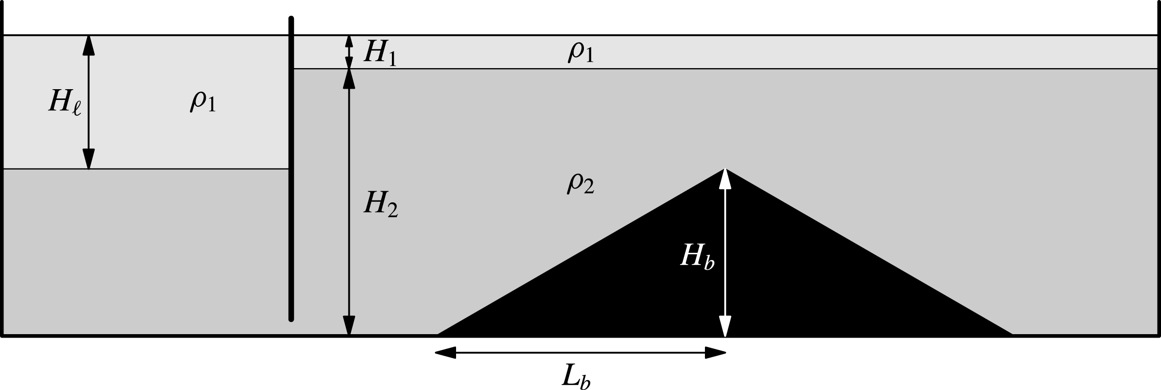
A schematic of the experimental set-up is shown in figure 2. The experiments were performed in a 197.3 cm long $\times$ 40 cm high $\times$ 17.3 cm wide glass tank. Before filling the tank, one of three different symmetric obstacles were inserted: a ‘thin’ vertical barrier, a ‘short’ triangular barrier or a ‘long’ triangular barrier. All were composed of 4 mm thick and 17.1 mm wide acrylic sheets with electrical tape and pieces of foam tape around the side to provide some friction between the acrylic and tank side walls while still permitting small ( ${<}1~\text{mm}$ ) gaps for water to flow through when filling the tank. We denote the height of the barrier by $H_{b}$ and the half-length of the barrier by $L_{b}$ . The barrier heights ranged between 5 and 25 cm, with most experiments having $H_{b}\simeq 20~\text{cm}$ . The maximum height of the topography was situated near the midpoint along the length of the tank. The barrier widths varied from $L_{b}\simeq 0.0~\text{cm}$ (for the ‘thin’ vertical barrier) to $L_{b}\simeq 48~\text{cm}$ (for the short triangular barrier) and $L_{b}\simeq 80~\text{cm}$ (for the long triangular barrier). In the case of the long barrier, we provided additional vertical supports in order to ensure that the slopes along the leading and trailing edges were constant.

Figure 2.

Schematic of the side view of the initial set-up of a lock–release experiment with triangular bottom topography.

With the barrier in place, blue-dyed salt water was poured into the tank to a prescribed depth. The salinity, measured with an Anton Paar DMA 4500 density meter, ranged from 1.0001 to $1.0500~\text{g}~\text{cm}^{-3}$ between different experiments. In all cases the depth of the salt water was larger than $H_{b}$ , so that the topography was completely submerged. Clear fresh water was then layered on top by pouring water through a sponge float. The generation of an internal solitary wave was accomplished through the standard lock–release method (Grue et al. Reference Grue, Jensen, Rusås and Sveen1999). A gate was inserted vertically between thin glass guides extending close to, but not touching, the bottom of the tank. This formed a lock, which in all experiments had length $L_{\ell }=28.7~\text{cm}$ . At this point more fresh water was poured through a sponge float in order to deepen the fresh water in the lock to a depth $H_{\ell }$ . In the process, the salt water at the bottom of the lock ran underneath the gate, moderately deepening the lower-layer depth of the ambient. This measured lower-layer depth was $H_{2}$ and the upper-layer depth was $H_{1}$ . In all experiments we set $H_{1}<H_{2}$ so that the generated solitary wave was one of depression, the interface displacing downwards from the relatively shallow upper layer. Values for $H_{1}$ ranged from 2.5 to 11 cm, with typical upper-layer depths around 5 cm. Values for $H_{2}$ ranged from 20 to 30 cm, with typical lower-layer depths around 20 cm. The depth, $H_{\ell }$ , of the fresh-water layer in the lock ultimately set the amplitude and lateral extent of the solitary wave. Typically, only one wave was generated as a consequence of the relatively small lock length (Sutherland et al. Reference Sutherland, Barrett and Ivey2013). Values of $H_{\ell }$ ranged from 7 to 30 cm.

For visualization purposes, two 4 mm thick translucent white plastic sheets were placed behind the tank and a bank of fluorescent lights was placed behind these. On the other side of the tank a camera was situated on a tripod approximately 3 m from the tank with the lens at the same height as the interface of the two-layer ambient and situated midway along the length of the tank. Movies were recorded using a Canon Rebel T3i camera.

At the start of an experiment, the gate was rapidly extracted vertically. Typically a single solitary wave of depression developed within one lock length from the gate. It was then observed as it interacted with the submerged topography. By design, in most experiments the wave was observed to break partially against the barrier with some energy transmitting across it and some reflecting back from it.

In all, 118 experiments were successfully performed. The incident solitary wave propagated at speeds between $C_{sw}\simeq 3$ and $15~\text{cm}~\text{s}^{-1}$ . The corresponding Reynolds number based upon $C_{sw}$ and $H_{1}$ ranged between 1500 and 18 000, with most experiments having Reynolds numbers between 5000 and 9000. In no experiments did we observe the development of Kelvin–Helmholtz billows arising from shear instability in the lee of the wave, as was observed by Fructus et al. (Reference Fructus, Carr, Grue, Jensen and Davies2009) in their experiments of solitary waves propagating along a thick interface. Because the energetics of the incident, transmitted and reflected waves were determined over an inspection window extending over a 1.5 m length, the effects of viscosity were not expected to play a significant role. This was confirmed by analysis of waves that interacted weakly with the barrier.

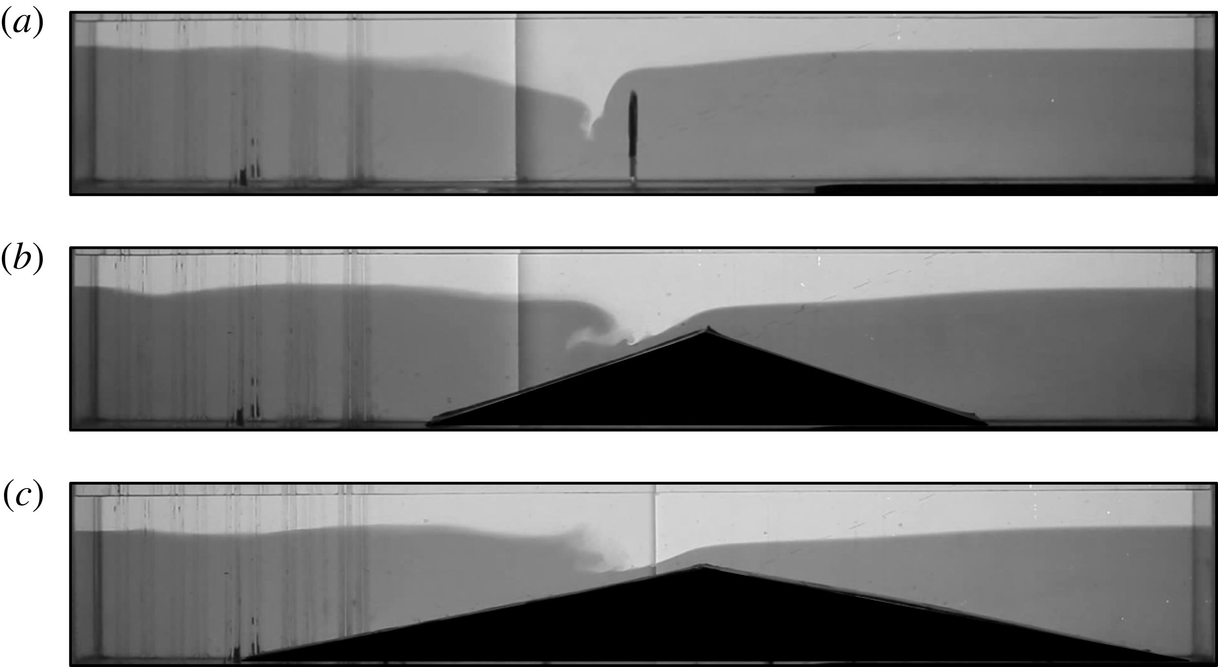
Snapshots taken from movies of experiments with thin, short and long topographic barriers are reproduced in figure 3 at a time when the solitary wave interacts with each type of barrier. In all three cases the incident solitary-wave amplitude was so large that the maximum upper-layer depth was comparable to the depth of the ambient above the ridge, $H_{1}+H_{2}-H_{b}\simeq H_{1}+A_{sw}\simeq 12~\text{cm}$ .

Figure 3.

Successive snapshots from experiments in which a solitary wave approaches (a) a thin barrier (see supplementary movie 1, available at http://dx.doi.org/10.1017/jfm.2015.306), (b) a short barrier (see supplementary movie 2) and (c) a long barrier (see supplementary movie 3). In all three experiments, $H_{1}\simeq 5.5~\text{cm}$ , $H_{2}\simeq 21.5~\text{cm}$ , $g^{\prime }\simeq 22~\text{g}~\text{cm}^{-3}$ , $H_{\ell }=15.5~\text{cm}$ , $H_{b}=15.0~\text{cm}$ and the measured incident solitary-wave amplitude is $A_{sw}\simeq 6.5~\text{cm}$ . The measured transmission and reflection coefficients are $T=0.33$ and $R=0.20$ , $T=0.49$ and $R=0.09$ , and $T=0.52$ and $R=0.08$ , respectively, for the thin-, short- and long-barrier experiments. Typical measurement errors for $T$ and $R$ are $\pm 0.03$ .

As each wave approached the barrier, the upper layer over the ridge deepened while the lower layer became more shallow. As a consequence, the return flow in the lower-layer ambient became constrained to pass though an increasingly narrow region. In the thin-barrier experiment, the leftward lower-layer flow interacted with the rightward upper-layer flow of the approaching wave such that the interface on the facing side of the barrier plunged to great depth (figure 3 a). This resulted in turbulent mixing between the upper- and lower-layer ambient fluid, behaviour similar to that observed by Maderich et al. (Reference Maderich, Talipova, Grimshaw, Terletska, Brovchenko, Pelinovsky and Choi2010) in their study of a solitary wave approaching step-shaped topography.

In the short-barrier experiment, the constrained lower-layer flow over the top of the barrier ran downslope, eventually separating from the boundary (figure 3 b). At the same time, because the trailing flank of the solitary wave was in relatively deeper water, it caught up to the leading flank and overturned. The simultaneous boundary-separated flow with overturning aloft was observed in some of the experiments of Sveen et al. (Reference Sveen, Guo, Davies and Grue2002) and Vlasenko & Hutter (Reference Vlasenko and Hutter2002), and has since been classified as a ‘collapsing–plunging’ breaker (Boegman et al. Reference Boegman, Ivey and Imberger2005; Sutherland et al. Reference Sutherland, Barrett and Ivey2013).

In the long-barrier experiment shown in figure 3(c), the structure of the breaking wave appears predominantly as a plunging breaker with less evidence of boundary layer separation of the opposing downslope lower-layer flow (figure 3 c).

In all three cases, some mixing occurred to the left of the ridge as the waves interacted with the barrier. But then the flow partially surged over the barrier, launching rightward-propagating interfacial waves on the other side. Meanwhile, reflected leftward-propagating waves were also evident.

Figure 4.

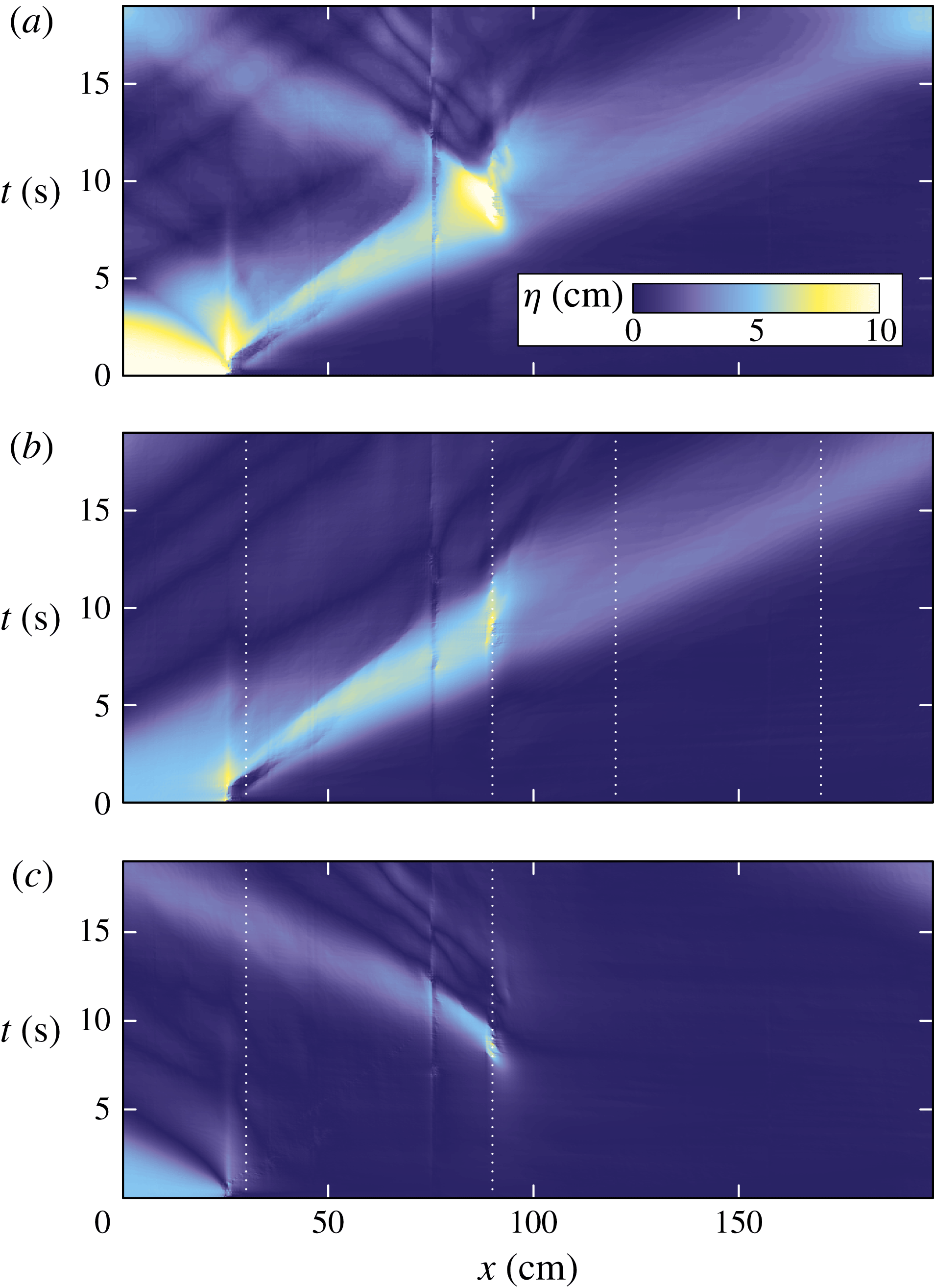
(a) Time series showing the downward displacement of the interface along the length of the tank for the thin-barrier experiment shown in figure 3(a). This field is Hilbert-transformed to show the displacement associated with (b) rightward- and (c) leftward-propagating disturbances. The vertical white dotted lines in (b) denote the typical extents of the left and right windows used to measure the energy of incident and transmitted waves. The vertical white dotted lines in (c) denote the typical extent of the window used to measure the energy of reflected waves.

The transmitted and reflected waves were clearly evident in time series of the measured interface displacement, ${\it\eta}(x,t)$ . For example, figure 4(a) shows the time series corresponding to the thin-barrier experiment shown in figure 3(a). To produce this figure, the displacement of the interface at each snapshot in time was found by importing successive frames from the movie into MatLab and finding the position of the contour where the intensity between the relatively dark-dyed lower layer and clear upper layer changed most rapidly. The downward displacement of the contour from the initial level of the interface in the ambient outside the lock is denoted by ${\it\eta}(x,t)$ . In constructing ${\it\eta}$ , there was some difficulty extracting reliable values at the horizontal position where the two white plastic sheets behind the tank were abutted together (at $x=78~\text{cm}$ for this experiment). Because the error in the measurement of ${\it\eta}$ is localized about this position, it could be filtered from measurements used to determine the wave energetics.

The Hilbert transform methodology of Mercier, Garnier & Dauxois (Reference Mercier, Garnier and Dauxois2008) is used to separate ${\it\eta}$ into the displacements ${\it\eta}_{R}$ and ${\it\eta}_{L}$ associated respectively with the rightward- and leftward-propagating disturbances. The results are shown in figure 4(b,c). Note that the initial disturbance in the lock (between $x=0$ and 28.7 cm) becomes decomposed into the superposition of rightward- and leftward-propagating waves, consistent with this stationary displacement being represented as a standing wave. Between $t=4$ and 8 s the disturbance in the tank is composed entirely of rightward-propagating waves. Thereafter this disturbance continues rightwards, though at smaller amplitude, while the generation of a leftward-propagating wave is evident at the location of maximum interfacial deepening to the left of the barrier.

From ${\it\eta}_{R}(x,t)$ and ${\it\eta}_{L}(x,t)$ , we characterized the energy associated with the incident, transmitted and reflected waves and so found transmission and reflection coefficients for a solitary wave of depression passing over a submerged barrier. We chose to characterize the energy of the waves in terms of their available potential energy alone. This is defined directly in terms of the interface displacement, ${\it\eta}$ , in a Boussinesq fluid by

which is the available potential energy per unit horizontal area.

To calculate the time evolution of the energy associated with propagating waves alone, we integrate $\mathscr{A}$ horizontally only within windows that exclude the lock, the region around the peak of the barrier where significant plunging and mixing of the interface occurs, and the rightmost region of the tank where the transmitted wave reflects off the endwall. Thus we define the available potential energy per unit width associated with rightward-propagating waves to be

and that associated with the leftward-propagating waves to be

in which $\mathscr{A}_{+}$ and $\mathscr{A}_{-}$ are given by (3.1) with ${\it\eta}$ in the integrand replaced by ${\it\eta}_{R}$ and ${\it\eta}_{L}$ , respectively. The choice of the windowing ranges, $[x_{1},x_{2}]$ and $[x_{3},x_{4}]$ , varies between experiments depending upon the positioning and type of topographic barrier used. Typically, we set $x_{1}=30~\text{cm}$ , $x_{2}=90~\text{cm}$ , $x_{3}=120~\text{cm}$ and $x_{4}=170~\text{cm}$ . Within these windows, the interface remains sharp, with the transition from the clear (upper-layer) and dark (lower-layer) fluid to the midpoint of the interface occurring typically over a distance of 2 mm (the vertical extent scale of 2 pixels of the digitized images). Taking the error in measurements of ${\it\eta}$ to be half this distance, the corresponding uncertainty is of the order of 2 % of the typical transmitted and reflected wave amplitudes. This suggests errors of the order of a few per cent in the measurement of $\mathscr{E}_{A+}$ and $\mathscr{E}_{A-}$ due to errors associated with the measurement of  ${\it\eta}$ .

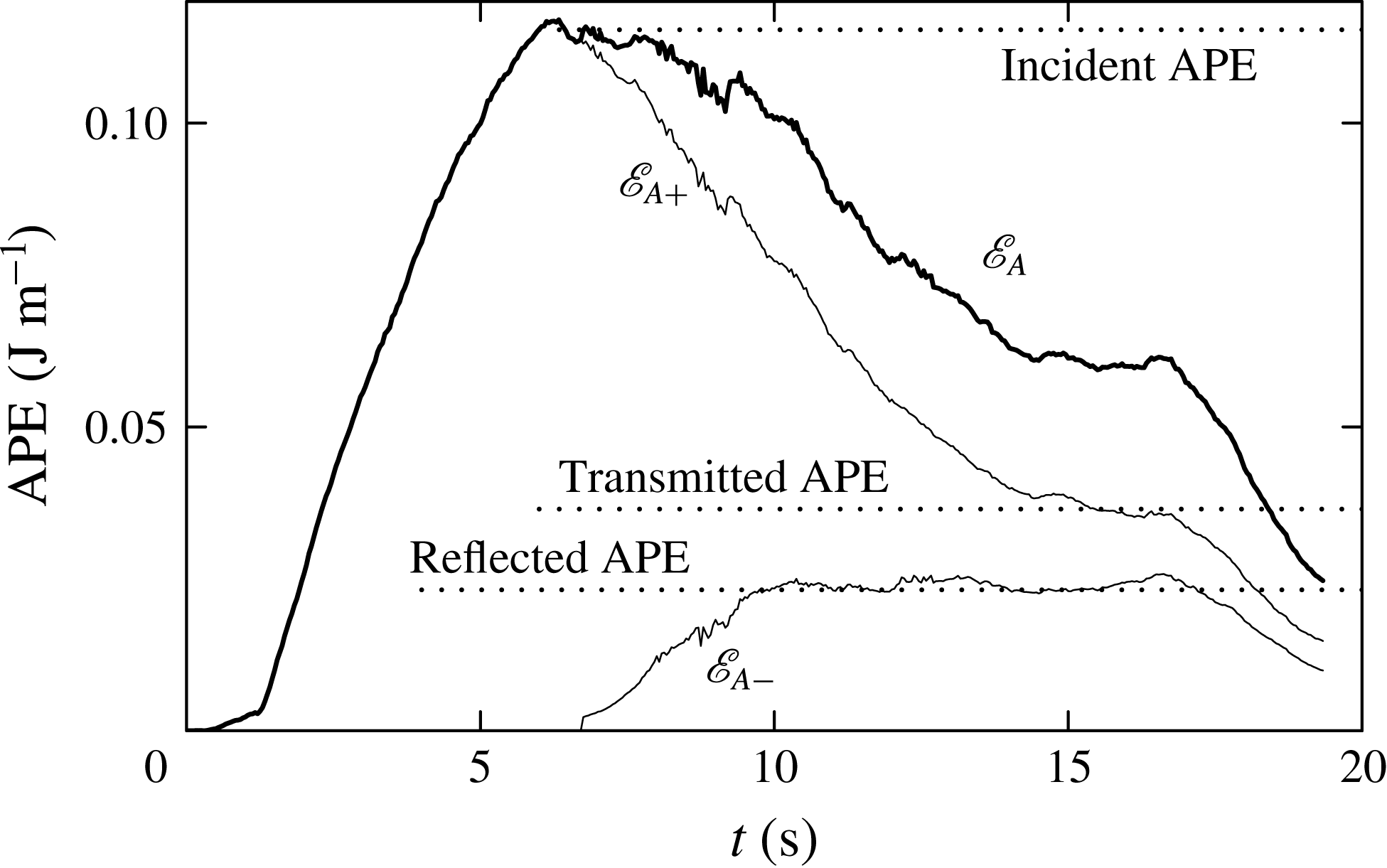
Figure 5 plots values of the available potential energy per unit width computed for the experiment of a solitary wave approaching a thin barrier, as shown in figure 3(a). Shortly after $t=0~\text{s}$ , the total available potential energy increases as the rightward-propagating wave moves into the analysis window, $[x_{1},x_{2}]$ . The energy peaks around 6 s, which is the time when the disturbance begins to propagate out the right side of the window and the wave itself begins to interact with the barrier. Shortly after this time, the available potential energy associated with the leftward-propagating wave grows as the waves propagate from the right into the window $[x_{1},x_{2}]$ . The values of $\mathscr{E}_{A-}$ and $\mathscr{E}_{A+}$ both plateau and then decrease after $t=17~\text{s}$ when the leftward- and rightward-propagating waves leave their respective interrogation windows.

Figure 5.

Evolution of the horizontally integrated available potential energy (APE) per unit width computed from the displacement fields of rightward- and leftward-propagating disturbances as shown in figure 4(b,c). The energy associated with rightward-propagating waves is given by (3.2) with $[x_{1},x_{2}]=[30,90]$ and $[x_{3},x_{4}]=[120,170]$ . The energy associated with leftward-propagating waves is given by (3.3) with $[x_{1},x_{2}]=[30,90]$ . The total energy, which is the sum of $\mathscr{E}_{A+}$ and $\mathscr{E}_{A-}$ , is plotted as the thick solid line. The horizontal dotted lines indicate the particular values associated with the incident, transmitted and reflected waves. For this experiment, the measured transmission and reflection coefficients are $T=0.33$ and $R=0.20$ , respectively.

The behaviour shown in figure 5 is typical of most of our experiments. From such graphs, we define the ‘incident available potential energy’, $E_{I}$ , to be the maximum available potential energy per width associated with the rightward-propagating wave. The average of $\mathscr{E}_{A-}$ over the time where it plateaus is called the ‘reflected available potential energy’, $E_{R}$ . The average of $\mathscr{E}_{A+}$ over the later time when it plateaus is called the ‘transmitted available potential energy’, $E_{T}$ . These values are indicated by the dotted lines in figure 5.

From these values, we define the transmission and reflection coefficients to be

The typical error in these measurements was $\pm 0.03$ as determined by the standard deviation of $\mathscr{E}_{A+}$ and $\mathscr{E}_{A-}$ over regions where the energies plateaued.

From the theory in § 2, an internal solitary wave is predicted to be unstable if its amplitude exceeds a critical value $A_{c0}$ , given by (2.10). If the incident wave amplitude $A_{sw}$ is much smaller than $A_{c0}$ measured above the ridge, the wave is expected to transmit with negligible breaking or reflection, as if the barrier was not present. However, if $A_{sw}$ is much larger than $A_{c0}$ , the transmission is expected to reduce significantly as a result of instability. Although we cannot expect to derive an analytic formula for the transmission and reflection coefficients as a function of $A_{sw}/A_{c0}$ , we anticipate that the coefficients should change significantly as $A_{sw}/A_{c0}$ changes from small to large values, with the transition occurring around $A_{sw}/A_{c0}\sim 1$ .

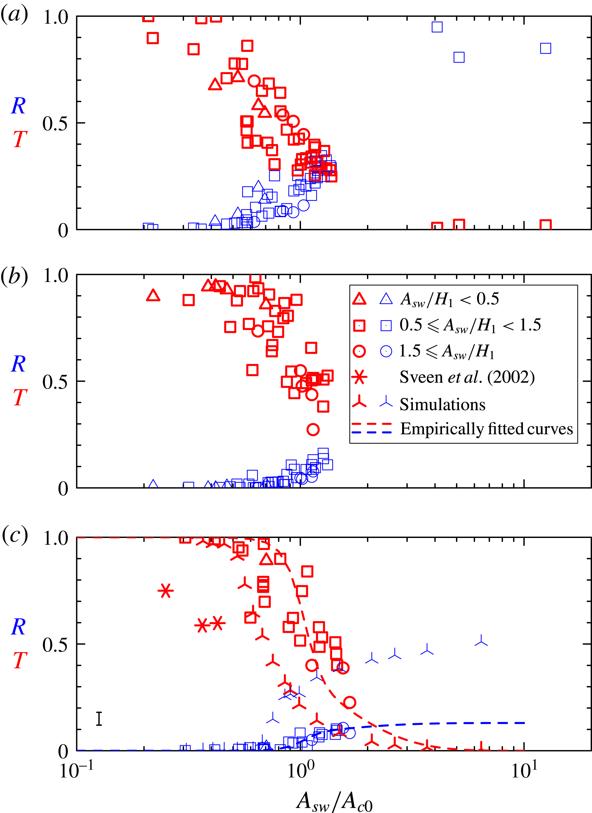
Figure 6 plots the measured transmission and reflection coefficients against $A_{sw}/A_{c0}$ separately for experiments with the thin, short and long barriers. As a measure of the nonlinearity of the incident wave, different symbols are plotted depending on whether $A_{sw}/H_{1}<0.5$ (weakly nonlinear; triangles), $0.5\leqslant A_{sw}/H_{1}<1.5$ (moderately nonlinear; squares) and $A_{sw}/H_{1}>1.5$ (strongly nonlinear; circles). In each plot, transmission coefficients are plotted as thick symbols (red online) and reflection coefficients are plotted as thin symbols (blue online).

Figure 6.

Transmission (thick symbols; red online) and reflection (thin symbols; blue online) coefficients determined from laboratory experiments plotted against the incident wave amplitude relative to the critical amplitude $A_{c0}$ predicted by theory. Values are shown separately for experiments with (a) a thin barrier, (b) a short barrier and (c) a long barrier. In all three plots the triangles, squares and circles denote the amplitude of the incident wave relative to the upper-layer depth, as indicated in the legend in (b). In (c) we also plot by stars the transmission data of Sveen et al. (Reference Sveen, Guo, Davies and Grue2002) and by ‘turnstiles’ the results of simulations reported in § 4. Empirical fits to the transmission and reflection data of the long-barrier experiments are plotted in (c) according to equations (5.1) and (5.2) with parameters given in table 1. The typical error in measurements is indicated by the error bar to the lower left in (c).

Consistent with expectations, we find that the measured transmission coefficients are near unity and reflection coefficients are near zero if $A_{sw}/A_{c0}$ is sufficiently small. Transmission drops rapidly as $A_{sw}/A_{c0}\gtrsim 1$ . Despite some scatter in the data, which we attribute to the choice of windowing used to measure the available potential energy of the incident, transmitted and reflected waves, the data show reasonably good collapse when plotted against $A_{sw}/A_{c0}$ . In particular, there is no significant dependence of $T$ and $R$ upon the amplitude of the incident wave relative to the upper-layer depth. There is a qualitative difference between the dependence of $T$ and $R$ upon $A_{sw}/A_{c0}$ between the thin-barrier and the short- and long-triangular-barrier cases. The transmission of waves across a thin barrier decreases significantly from unity if $A_{sw}/A_{c0}$ is greater than 0.4, and wave reflection becomes evident if $A_{sw}/A_{c0}$ is greater than 0.6 (figure 6 a). For waves approaching either the short or long triangular barrier, we find that transmission decreases significantly from unity if $A_{sw}/A_{c0}$ is greater than 0.5–0.6, and wave reflection becomes evident only as $A_{sw}/A_{c0}$ exceeds 0.9. Even with $A_{sw}/A_{c0}\simeq 1.5$ , transmission remains relatively large, with $T\simeq 0.4\pm 0.1$ , and reflection is small, with $R\simeq 0.1\pm 0.05$ . The reflection coefficient is moderately smaller than that found by Michallet & Ivey (Reference Michallet and Ivey1999), who estimated $R$ to lie in the range 0.2–0.3, with large slopes having $s\simeq 0.169$ . But $R$ is an order of magnitude larger than the value estimated by Sveen et al. (Reference Sveen, Guo, Davies and Grue2002) resulting from strong wave–barrier interactions. Perhaps this is because the experiments for which they examined reflection did not access the regime with $A_{sw}/A_{c0}>1$ .

Figure 6(c) also plots as stars the transmission coefficients from data provided in Sveen et al. (Reference Sveen, Guo, Davies and Grue2002). In all three cases the topographic slope was 0.1, approximately half that of our long-barrier experiments. Although $A_{sw}/A_{c0}<0.5$ (and $A_{sw}/(H_{2}-H_{b})<0.5$ ) in all cases, they observed substantially less transmission than our experiments would suggest. Comparison of our short- and long-barrier experiments and the numerical results we present later suggests that their relatively low transmission is not a consequence of the lower slope in their experiments. Indeed, our simulations show that transmission increases with decreasing slope. Part of the discrepancy may be due to our definition of the reflection coefficient in terms of available potential rather than total energy. But our numerical simulations suggest that this would result in at most a 5 % change. More likely is the fact that Sveen et al. (Reference Sveen, Guo, Davies and Grue2002) measured the transmitted wave energetics far from the barrier and the heuristics they used to account for viscous attenuation of the leading pulse and trailing waves did not accurately estimate the true loss due to viscosity.

There is no significant difference in the dependence of $T$ and $R$ upon $A_{sw}/A_{c0}$ between the short- and long-barrier cases. Even though the long barrier still has large slope ( $\simeq 0.19$ ) relative to typical slopes ( ${\lesssim}0.1$ ) occurring below the coastal oceans, the results of these experiments suggest that they may be extended to oceanographic circumstances. The dependence of topographic slope upon the transmission and reflection of ocean-scale waves is examined in more detail through results of numerical simulations presented in the next section.

4. Numerical simulations

Numerical simulations were performed using a code, generously provided by Kevin Lamb, which solves the fully nonlinear Navier–Stokes equations in two dimensions using finite differences on a terrain-following coordinate system (Lamb Reference Lamb1994; Lamb & Yan Reference Lamb and Yan1996). This has been used in the study of large-amplitude internal solitary waves (Lamb Reference Lamb2002; Lamb & Wilkie Reference Lamb and Wilkie2004), the shoaling of internal solitary waves upon a uniform slope (Aghsaee et al. Reference Aghsaee, Boegman and Lamb2010) and the bottom boundary layer stresses and flow separation that results from a solitary wave of depression passing over a uniform-depth ambient (Aghsaee et al. Reference Aghsaee, Boegman, Diamessis and Lamb2012). Here the code is used to simulate experiments of internal solitary waves incident upon triangular barriers and to simulate circumstances more representative of oceanic phenomena.

The background density is prescribed to be a two-layer fluid with finite-depth interface, $D$ , at depth $z=-H_{1}$ according to

To simulate flow over a triangular ridge while avoiding sharp gradients, the bottom topography was approximated so that the height above the bottom was given by the following sum of analytic functions:

Here ${\it\epsilon}=0.02$ sets the (small) relative transition between flat and sloping segments of each curve and we have arbitrarily centred the hill at $x=0$ .

Rather than simulating the evolution of the solitary wave after its release from a lock, we used the iterative procedure of Lamb (Reference Lamb2002) to initialize the simulations with a single solitary wave using the computed solution of the Dubreil-Jacotin–Long equation (Dubreil-Jacotin Reference Dubreil-Jacotin1937; Long Reference Long1953, Reference Long1956; Lamb Reference Lamb2002; White & Helfrich Reference White and Helfrich2008):

in which $N^{2}$ is the squared buoyancy frequency associated with the background stratification. If the solitary wave moves at speed $c$ through an otherwise stationary ambient, ${\it\xi}(x,z)$ describes the displacement of streamlines due to the wave taken in a frame of reference moving with the wave.

The code advances the simulation in time solving the fully nonlinear momentum and internal energy equations in the $x{-}z$ plane. The effects of viscosity and diffusion were included through the usual Laplacian operator. The kinematic viscosity was set to be that of water and the Schmidt number was 10, smaller than that of salt water, but inconsequential for the dynamics of the transmitted and reflected waves. In simulations of ocean-scale waves, viscosity and diffusion are included for numerical stability.

The equations were solved using finite differences on a staggered grid as described by Lamb (Reference Lamb1994). The horizontal domain extended from $x_{L}\equiv -300~\text{cm}$ to $x_{R}\equiv 300~\text{cm}$ with a resolution of $\text{d}x=L/3000=0.2~\text{cm}$ . The vertical resolution was $\text{d}z=H/100$ away from the model hill where the total ambient depth was $H$ , and the resolution was finer proportionally to the decreasing ambient depth over the hill. Fields were advanced in time by steps of 0.005 s typically up to $t=40~\text{s}$ when the transmitted and reflected waves had moved away from the model ridge.

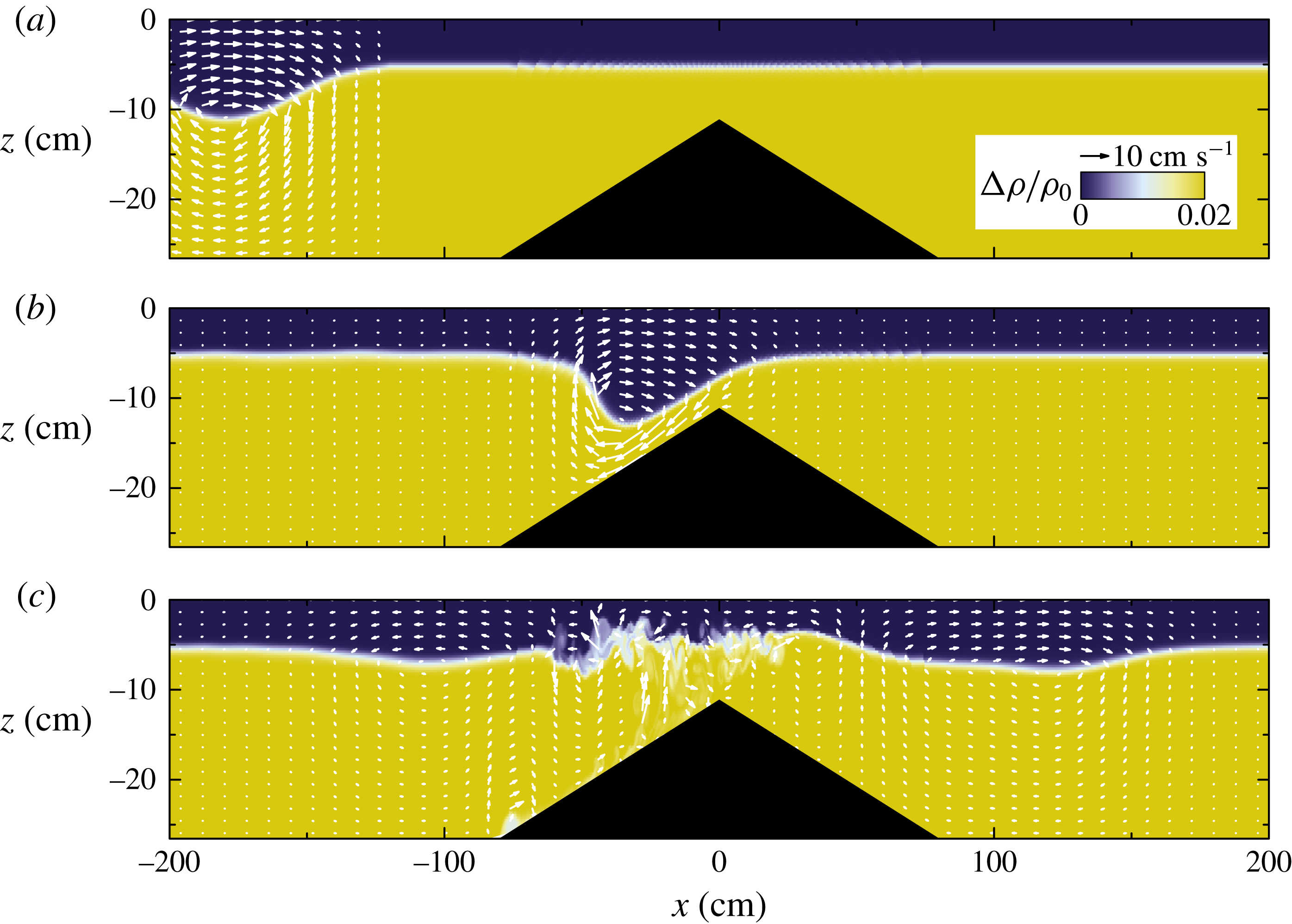
The snapshots shown in figure 7 are taken from a simulation run with parameters corresponding approximately to the experiment shown in figure 3(c).

Figure 7.

Snapshots at times (a) 0 s, (b) 15 s and (c) 30 s taken from numerical simulation with experimental parameters corresponding closely to those in figure 3(c) showing as a colour scale the relative difference of density from ${\it\rho}_{1}$ . The superimposed white arrows indicate velocity. The colour scale and magnitude of the velocity vectors are indicated in the legend in (a). (See supplementary movie 4.)

Initially the solitary wave is centred at $x=-180~\text{cm}$ having amplitude $A_{sw}=5.9~\text{cm}$ and half-length $L_{sw}=27.8~\text{cm}$ (figure 7 a). When interacting with the hill at $t=15~\text{s}$ (figure 7 b), it began its development into a plunging breaker, consistent with experimental observations (see figure 3 c). At this time, an upper-layer rightward flow on the far side of the barrier is apparent, while the lower-layer flow is observed to accelerate leftwards as it approaches the constriction above the peak of the hill. Because the simulation is restricted to two dimensions, it is not possible for the overturning fluid to break down into fully three-dimensional turbulence. Nonetheless, mixing was effective at eroding the small scales while preserving the formation of transmitted and reflected waves to either side of the barrier (figure 7 c).

As with the experiments, we performed an analysis of energetics to measure the relative energy associated with the transmitted and reflected waves. From the density field we determined the available potential energy density as the difference of the potential energy in the presence of perturbations from the undisturbed potential energy of the ambient. Explicitly, at any horizontal location, $x$ , we computed the available potential energy as

This is defined so that a parcel with zero potential energy is situated at $z=-H_{1}$ , the depth of the undisturbed interface. Doing so ensures that (4.4) reduces to the formula (3.1) in the limit of a two-layer fluid. Knowing the velocity field output by the simulations, the kinetic as well as available potential energy can be computed. In particular, the vertical integral of the kinetic energy is

For small-amplitude waves, $\mathscr{K}$ is expected to equal $\mathscr{A}$ . The simulations allow us to measure the magnitude of the departure from energy equipartition for the case of large-amplitude solitary waves.

To measure the kinetic and available potential energies associated with the incident, transmitted and reflected waves, we horizontally integrate the values of $\mathscr{K}$ and $\mathscr{A}$ within windows to the left and right of the hill. Specifically we define

in which ${\it\delta}=1.5$ is set so that the windows include wave-like behaviour while neglecting processes taking place over and near the barrier.

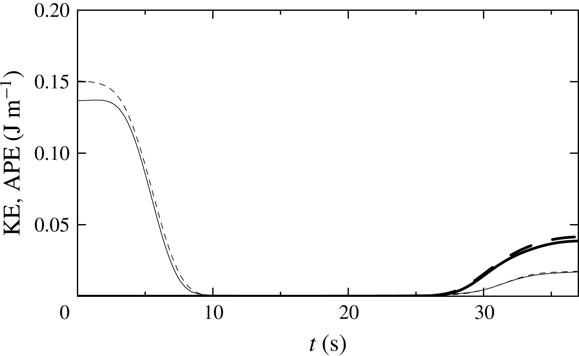
Figure 8 shows the time evolution of the kinetic and available potential energies computed in the windows to the left and right of the barrier. Initially, all the energy is contained within the left window. Here it is evident that the kinetic and available potential energies are close to equipartition, with $\mathscr{E}_{K-}=0.150~\text{J}~\text{m}^{-1}$ being just 10 % larger than $\mathscr{E}_{A-}=0.137~\text{J}~\text{m}^{-1}$ . Consistent with experiments, the computed available potential energy is of the order of that measured shortly after the wave was released from the lock. By $t=40~\text{s}$ the energy in each window is approximately constant and the kinetic and available potential energies associated with these smaller-amplitude waves are closer to equipartition.

Figure 8.

Temporal evolution of the available potential energy (APE; solid lines) and kinetic energy (KE; dashed lines) computed within windows extending leftwards from $-{\it\delta}L_{b}$ to the left of the barrier (thin lines) and rightwards from ${\it\delta}L_{b}$ to the right of the barrier (thick lines) computed from the simulation shown in figure 7. The transmission and reflection coefficients determined from available potential energy alone are $T=0.282$ and $R=0.124$ , respectively. The corresponding coefficients determined from total energy are $T=0.279$ and $R=0.120$ .

A sequence of simulations were performed with conditions similar to those of the laboratory experiments. The ambient fluid was set with upper- and lower-layer depths of 5.3 cm and 22.0 cm, respectively, and the half-depth of the interface was $D=0.5~\text{cm}$ . The incident solitary wave had amplitude $A_{sw}=5.9~\text{cm}$ and width $L_{sw}=27.8~\text{cm}$ centred at 180 cm to the left of the centre of the hill. The hill itself had fixed slope of $s=0.2$ and height that varied between simulations from $H_{b}=4.0$ to $H_{b}=21.0~\text{cm}$ .

The transmission and reflection coefficients are compared with results of the long-barrier experiments in figure 6(c). The simulations show a sharp decrease in the transmission coefficient as $A_{sw}/A_{c0}$ increases above $\simeq 0.6$ and an increase in the reflection coefficient to $\simeq 0.6$ for $A_{sw}/A_{c0}\gtrsim 6$ . Comparing this with the long-barrier experiments, we find that the transmission is close to the smallest values measured in experiments as $A_{sw}/A_{c0}$ ranged from small to large values. The reflection coefficient measured in simulations is significantly larger than that measured in experiments, probably because the simulations are restricted to two dimensions and so do not properly capture turbulent dissipation and mixing as the wave breaks upon the facing slope of the barrier.

The initialization of simulations of ocean-scale internal solitary waves was based upon the observations of waves in the South China Sea reported by Farmer et al. (Reference Farmer, Alford, Lien, Yang, Chang and Li2011). In these, the incident solitary-wave amplitude was set to be 142 m with width 386 m in an ambient with a thermocline with half-thickness 20 m centred 50 m below the surface. The ambient depth far from the hill was set to be $H=440~\text{m}$ . In different sequences of simulations, the half-width of the hill was set to be $L_{b}=2.5,~5,~10$ and 20 km. The hill heights ranged from $H_{b}=120$ to 368 m.

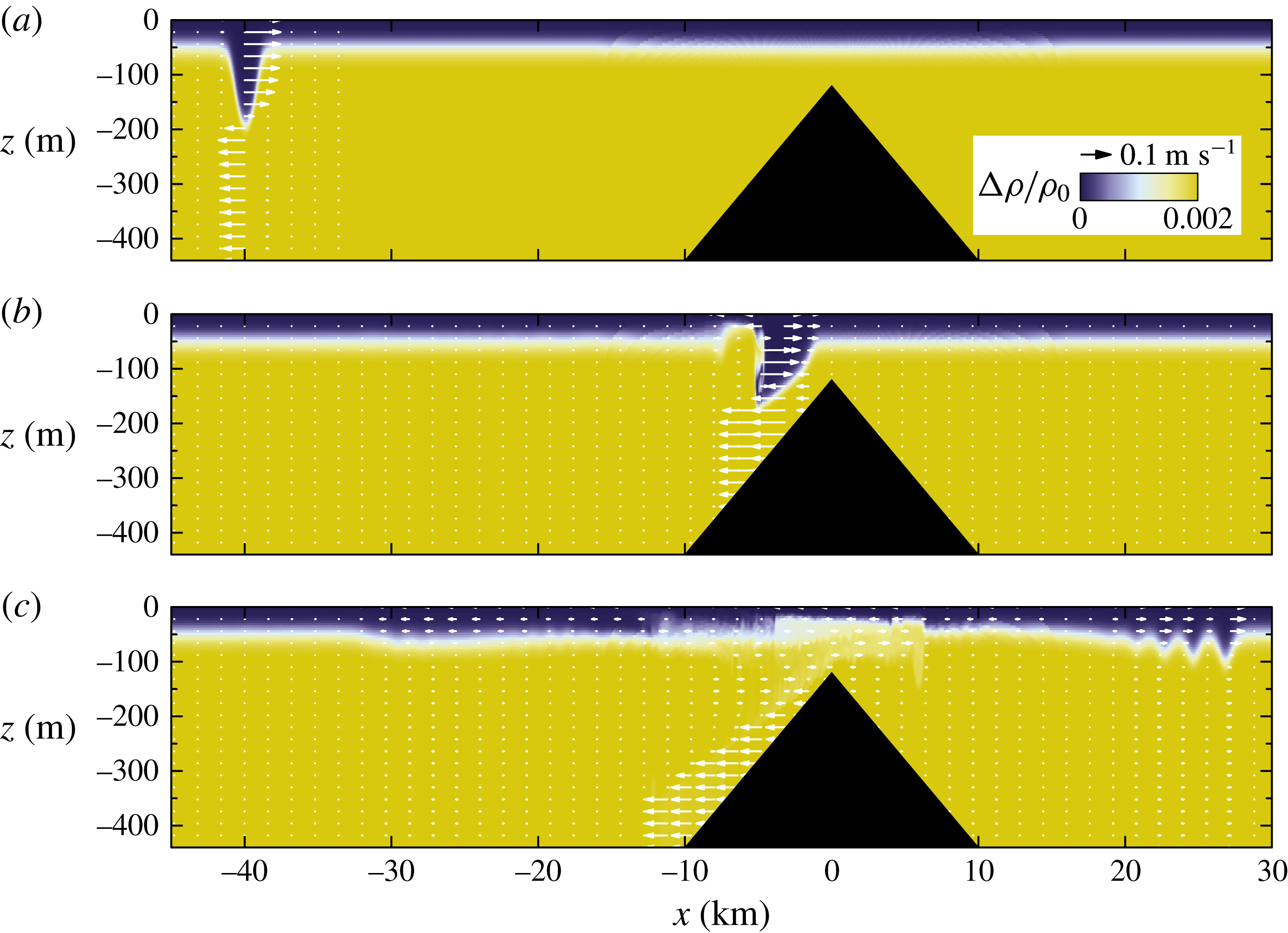
Snapshots from simulations with $L_{b}=10~\text{km}$ and $H_{b}=300~\text{m}$ are shown in figure 10. In this case, because the wavelength is comparable to the fluid depth, the flow is nearly uniform in the positive direction and nearly uniform in the negative direction, respectively, above and below the trough. The structure of the wave as it steepens is somewhat different from the experiment/simulations of the wave approaching the long barrier. Here the lee of the wave piles up as it approaches topography, making the upper layer more shallow. After passing over the ridge, a single long wave is reflected while the transmitted wave appears in the form of a wave train, consistent with the weakly nonlinear results of Grimshaw et al. (Reference Grimshaw, Pelinovsky, Talipova and Kurkin2004) and El, Grimshaw & Kamchatnov (Reference El, Grimshaw and Kamchatnov2007).

Figure 9.

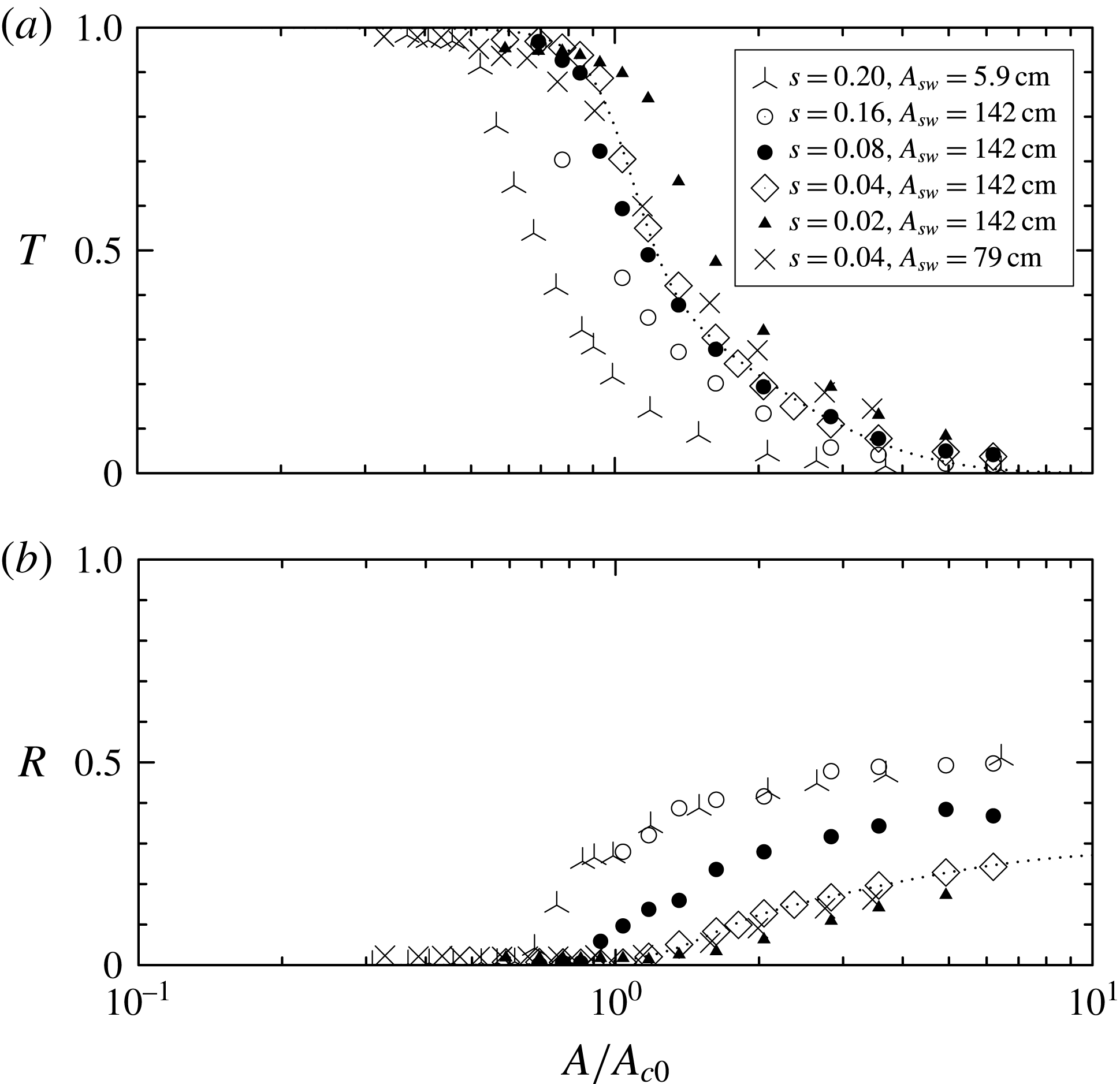
(a) Transmission and (b) reflection coefficients measured from numerical simulations of laboratory- and ocean-scale internal waves. Simulations of laboratory experiments (‘turnstiles’) are based upon the long-triangular-barrier experiment with ambient conditions given in figure 3(c) and with topographic slope 0.2 on either side of the ridge. The ocean-scale simulations have $H_{1}=50~\text{m}$ , $H_{2}=390~\text{m}$ and an incident wave with amplitude $A_{sw}=142~\text{m}$ and width $L_{sw}=387~\text{m}$ incident upon a ridge with slope $s=0.16$ (open circles), $s=0.08$ (closed circles), $s=0.04$ (open diamonds) and $s=0.02$ (closed triangles), and with amplitude $A_{sw}=79~\text{m}$ and width $L_{sw}=253~\text{m}$ incident upon a ridge with slope $s=0.04$ (crosses). In laboratory-scale simulations, the hill height ranges from 0 to 21 cm; these are the same data as those plotted as ‘turnstiles’ in figure 6. In ocean-scale simulations, the hill height ranges from $H_{b}=100$ to 368 m. The empirical fit to the sequence of simulations of ocean-scale waves with $A_{sw}=142~\text{m}$ and $s=0.04$ is shown by the dotted line.

Figure 10.

As in figure 7, but showing snapshots at times (a) 0 s, (b) 1500 s and (c) 3000 s taken from a numerical simulation of an ocean-scale incident solitary wave incident upon a ridge with half-width $L_{b}=10~\text{km}$ and height $H_{b}=300~\text{m}$ . (See supplementary movie 5.)

Figure 9 plots the reflection and transmission coefficients as a function of amplitude scaled by $A_{c0}$ . Although the amplitude and along-wave extent of the simulated ocean-scale waves are several orders of magnitude larger than those of the simulated laboratory-scale waves, the reflection coefficients are comparable when the topographic slope is relatively steep ( $s=0.16$ for ocean-scale waves and $s=0.20$ for laboratory-scale waves). However, the corresponding transmission coefficient for laboratory-scale waves is smaller. Transmission drops from $\simeq 0.8$ to 0.2 as $A/A_{c0}$ increases from $\simeq 0.6$ to 1.0. In comparison, for ocean-scale waves incident upon a topographic slope of 0.16, the transmission drops over this range as $A/A_{c0}$ increases from $\simeq 0.7$ to 1.6. This shift to higher transmission may be a consequence of the incident ocean-scale waves being long compared with the ambient depth far from topography such that the leftward flow at depth is significant.

For ocean-scale waves at fixed incident relative amplitude, it is clear that greater transmission occurs if the topographic slope is smaller. The sensitivity of the transmission coefficient to slope is most pronounced for $A_{sw}\simeq A_{c0}$ , with $T$ increasing successively by $\simeq 0.15$ as the slope decreases from $s=0.16$ to 0.08 to 0.04 to 0.02. Importantly, as in the laboratory experiments, the results do not depend sensitively upon the amplitude of the incident wave itself.

5. Empirical predictions

In an attempt to generalize these results, we have empirically fitted the data from experiments and simulations to analytic curves. The transmission coefficients were fitted to a curve that asymptotes exponentially to unity as $\tilde{A}\equiv A_{sw}/A_{c0}$ decreases to zero and that decreases exponentially to zero for large $\tilde{A}$ according to

The reflection coefficients were fitted to a curve that decreases exponentially to zero as $\tilde{A}$ decreases to zero and asymptotes exponentially to $R_{max}$ for large $\tilde{A}$ according to

In both cases, the results were most sensitive to the choices of $a_{t0}$ and $a_{r0}$ , which determine where $T$ and $R$ change most rapidly as $\tilde{A}$ changes. If ${\it\sigma}_{t-}\ll {\it\sigma}_{t+}$ , then ${\it\sigma}_{t-}$ determines the e-folding scale over which the transmission curve asymptotes to unity with decreasing $\tilde{A}$ , and ${\it\sigma}_{t+}$ determines the e-folding scale over which the transmission curve decreases exponentially to zero with increasing $\tilde{A}$ . A similar interpretation exists for the e-folding scales ${\it\sigma}_{r\pm }$ associated with the reflection curves.

For numerical simulations, a regression analysis was performed to find the best-fitting parameters for the $T$ and $R$ curves to simulations with fixed incident wave amplitude and topographic slope and with varying $\tilde{A}$ , which changed as a consequence of changing the height of the barrier. For the long-barrier experiments, the parameters were selected manually to produce order-of-magnitude correct values that reasonably produced a curve passing through the experimental data.

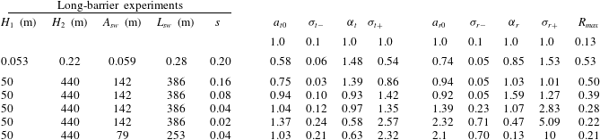
The parameters for experiments and simulations are listed in table 1. The resulting empirical fits to the transmission and reflection coefficient data measured in the long-barrier experiments are plotted as the dashed curves in figure 6(c). The dotted lines in figure 9(a,b) plot the empirical fits to the transmission and reflection coefficients determined in simulations of ocean-scale waves with a solitary wave of amplitude $A_{sw}=142~\text{m}$ incident upon a barrier with slope $s=0.04$ .

Table 1.

Coefficients of analytic curves in (5.1) and (5.2) used to fit measured transmission and reflection data measured in the long-barrier experiments (top row below header) and in numerical simulations using experiment scales (next row) and oceanic scales (bottom five rows).

Comparing the first two rows of data, we can make a quantitative comparison between the long-barrier experimental results and the results of simulations run with comparable parameters. The relatively low value of $a_{t0}=0.58$ determined from the simulations shows that the transmission begins to drops off at smaller values of $\tilde{A}$ , and the larger value of $R_{max}=0.53$ indicates that more energy is reflected than dissipated in simulations with waves that strongly interact with the barrier. As stated above, we attribute the discrepancy to unrealistic representation of turbulence in a two-dimensional model.

The parameters determined for ocean-scale waves give a quantitative measure of the effect of incident wave amplitude and topographic slope upon transmission and reflection coefficients. Comparing the two simulations with slope $s=0.04$ and with incident amplitudes 79 and 142 m, we see little difference in the values of $a_{t}$ , which most significantly controls the transition amplitude from strong to weak transmission. The value of $a_{t}$ does vary with slope, increasing from 0.75 to 1.37 as the slope decreases from $s=0.16$ to 0.02.

Finally, we may use our predicted value for the maximum reflection coefficient $R_{max}$ (occurring in the limit of a barrier that penetrates through the interface) to the predictions of wave reflection from a uniform slope (Bourgault & Kelley Reference Bourgault and Kelley2007; Aghsaee et al. Reference Aghsaee, Boegman and Lamb2010).

Fitting an exponential to the values of $1-R_{max}$ versus the Iribarren number (1.1), we find $R_{max}=1-\exp [-\mathit{Ir}/(0.33\pm 0.05)]$ . The e-folding value is about half that estimated by Aghsaee et al. (Reference Aghsaee, Boegman and Lamb2010). The discrepancy could be because our results are based on very large-amplitude ocean-scale waves. But it may also be that the dynamics of wave breaking and reflection differ quantitatively when the topographic barrier penetrates through the interface and surface.