Nomenclature
- A
-
area
 $[\mathrm{m}^2]$
- B
-
heat coefficient
$[\mathrm{J}/(\mathrm{kg}^2)]$
- C
-
specific heat [J/(kg·K)]
-
${C_p}$
-
specific heat at constant pressure [J/(kg·K)]
-
${C_v}$
-
specific heat at constant volume [J/(kg·K)]
- D
-
diameter [m]
- E
-
energy [J]
- e
-
specific energy [J/kg]
- f
-
friction coefficient [dimensionless]
- H
-
enthalpy [J]
- h
-
specific enthalpy [J/kg]
- L
-
length [m]
- M
-
mass [kg]
- P
-
pressure [Pa]
- R
-
specific gas constant [J/(kg·K)]
- T
-
temperature [K]
- t
-
time [s]
- V
-
volume
$[\mathrm{m}^3]$
- v
-
velocity [m/s]
-
$\dot m$
-
mass flow rate [kg/s]
-
$\dot q$
-
thermal power [W]


Greek symbol
-
$\gamma $
-
specific heat ratio [dimensionless]
-
$\rho $
-
density [kg/m
${}^3$
]


Subscripts
- I
-
integral
- n
-
nozzle
- p
-
plenum
- pipes
-
pipes
- r
-
reservoir
- v
-
valve
- va
-
valve adiabatic
- vi
-
valve inlet
1.0 Introduction
Despite being used for over a century, supersonic wind tunnel facilities remain a fundamental research tool for high-speed aerodynamics, thanks in part to recent advancements in laser-based diagnostics that have significantly augmented experimental research capabilities. Among these facilities, blow-down tunnels are among the most widely used because they can maintain controlled conditions for longer test durations, often lasting several seconds or even minutes, despite typically being limited to lower Mach numbers due to heating constraints.
A blow-down supersonic wind tunnel works by accumulating high-pressure gas in a reservoir and discharging it through a converging-diverging nozzle to achieve the desired velocities. Except from the simplest facilities, the nozzle is not connected directly to the reservoir, but rather to a secondary chamber, the plenum. A pressure-regulating valve between the reservoir and the plenum helps maintain constant pressure in the latter, allowing for steady testing conditions as long as the reservoir pressure remains higher than the desired plenum pressure. However, accurately predicting and controlling these testing conditions requires sophisticated mathematical models that capture the unique characteristics of each tunnel design.
A number of authors have developed mathematical models to address the specific challenges of supersonic wind tunnels operation. Since these facilities are largely unique, each one presents specific challenges that have prompted the development of a variety of models. One of the first numerical models of a supersonic wind tunnel is that of Fung et al. [Reference Fung, Settles and Ray1]. In their work the authors develop a system of four differential equations based on conservation of mass and energy in the reservoir and plenum, respectively. The authors assumed isentropic flow with no heat addition or pressure losses. Their model, applied to the Penn State Supersonic Wind Tunnel Facility, showed good results when compared to experimental measurements of the plenum pressure.
Hwang and Hsu [Reference Hwang and Hsu2] present a similar numerical model of a blow-down supersonic wind tunnel. This model incorporates differential mass conservation principles in both the reservoir and plenum, alongside energy conservation in the plenum. The authors assumed again adiabatic flow, and a choked control valve. However, they did not provide a comparison of the model with experimental values.
Braun et al. [Reference Braun, Lu, Panicker, Mitchell, Wilson and Dutton3] developed a combined tunnel-controller model that employs a PI-type controller and numerically solves for the valve opening equation. In this model, the authors assume an isothermal process. While a pressure loss coefficient is included in the equations, it remains unclear whether this coefficient was derived from previous experimental measurements. The authors compare one experimental test case with a simulation generated from their model, demonstrating that it predicts the tunnel’s plenum pressure well; however, the experimental reservoir pressure results are significantly higher than those predicted from the model.
Silva et al. [Reference Silva, Gamarra and Koldaev4] developed a model similar to that of Fung et al. [Reference Fung, Settles and Ray1] (comprising four differential equations with isentropic flow). However, they modified it to account for their nozzle’s variable geometry. In this case, the authors focused on developing a controller to maintain a constant Reynolds number rather than a constant total pressure. They compared their numerical predictions with various experimental tests and noted that the differences were likely due to the erroneous assumption of adiabatic flow. To validate their model, the authors compared its predictions with those of Fung et al. [Reference Fung, Settles and Ray1].
Ilić et al. [Reference Ilić, Miloš and Isaković5, Reference Ilić, Miloš, Milosavljević and Isaković6] present a model based on four differential equations, which account for the conservation of mass and energy in the reservoir and plenum, respectively. This approach is similar to that of Fung et al. [Reference Fung, Settles and Ray1]. However, the key difference between the two models lies in how the flow through the control valve is modeled. Fung et al. rely on the gas sizing coefficient provided by the valve manufacturer, while Ilić et al. use an analytical approach based on continuity and isentropic flow, introducing an experimentally determined coefficient to account for losses (up to 1.6). Despite this modification, all processes are still considered isentropic. The results of this work demonstrate very good agreement between the simulated and experimental pressure traces in both the plenum chamber and reservoir.
Huang [Reference Huang7] developed a numerical model for a short-duration blow-down wind tunnel. This model assumes isentropic flow and, more importantly, posits that the mass flow rate between the control valve and the nozzle throat is always equal. This assumption leads to a simple analytical equation that expresses valve opening as a function of time. Huang subsequently expanded the model by incorporating time derivatives of both reservoir and plenum pressures, which allowed for analytical solutions to be derived. The model was then utilised to train a PID controller. However, the author did not compare the model’s predictions with experimental results.
A key characteristic of cold-flow wind tunnels is thermal drift. As the working gas in the reservoir expands it also cools. This results in lower plenum, and consequently total, temperatures over time. This temperature drop directly impacts flow velocity and the Reynolds number in the test section, both of which become variable during testing due to thermal drift. The extent of this effect depends on specific design and operational characteristics of each facility; however, temperature drops of 110 K have been reported as a common occurrence [Reference Pope and Goin8].
Pope [Reference Pope and Goin8] discussed thermal drift and how the gas expansion in the reservoir doesn’t follow an ideal adiabatic process. The thermal mass of the reservoir and pipes transfers heat to the gas, reducing the expected temperature drop. To account for this, Pope used a polytropic expansion coefficient, which is facility-specific and must be determined experimentally. Despite Pope’s critical insight, subsequent numerical models have often overlooked this factor, commonly assuming adiabatic expansion [Reference Fung, Settles and Ray1, Reference Hwang and Hsu2, Reference Silva, Gamarra and Koldaev4, Reference Ilić, Miloš, Milosavljević and Isaković6, Reference Huang7] or, in some cases, even isothermal conditions [Reference Braun, Lu, Panicker, Mitchell, Wilson and Dutton3]. While these assumptions may be reasonable for certain wind tunnels under specific conditions, they generally fail to account for the significant impact of heat addition, potentially leading to inaccuracies in modeling and performance predictions. For example, in a Mach 3 facility operating at constant plenum pressure, a temperature drop of 50 K (less than half of what is reported as common [Reference Pope and Goin8]) results in a 34% increase in Reynolds number.
In addition to heat addition, real gas effects have also been overlooked in previous models of blow-down wind tunnels. For example, Joule–Thomson effect leads to a temperature drop (typically) across the pressure control valve. This effect describes the temperature change of a gas during an isenthalpic expansion, a phenomenon well-documented in early literature on wind tunnel design [Reference Pope and Goin8–Reference Lukasiewicz11]. The extent of Joule–Thomson effect depends primarily on the pressure drop across the regulating valve. For example, facilities with moderate reservoir pressures (approximately 2 MPa) experience temperature changes on the order of a fraction of a degree [Reference Pope and Goin8], however, for high-pressure reservoirs (11 MPa) the temperature drop is approximately 15 K. Despite this significance, the Joule–Thomson effect has been neglected in modern numerical models, which may lead to inaccuracies in temperature predictions during testing.
Vuković and Damljanović [Reference Vuković and Damljanović12] describe the problem of temperature drop for blow-down facilities, focusing on how thermal balances are affected by changes in test section temperature. They identify two primary effects contributing to thermal drop: gas expansion in the reservoir tanks (modeled with a polytropic expansion) and the Joule–Thomson effect. The latter describes the temperature drop that occurs when a gas is expanded through a valve, specifically the regulating valve in this context.
The discussed literature has primarily focused on developing models aimed at testing control strategies for wind tunnels. Most studies emphasised maintaining a constant pressure in the plenum chamber, resulting in temperature being a secondary consideration. An exception to this trend is the work of Silva et al. [Reference Silva, Gamarra and Koldaev4], where the authors aimed to develop a controller to maintain a constant Reynolds number, thus making temperature a key factor in their model. However, they still assumed isentropic flow and did not provide any experimental comparison regarding temperature predictions.
Consequently, there is a notable lack of information regarding temperature modeling in blow-down supersonic wind tunnels. Accurately modeling temperature is essential for several key aspects of wind tunnel operation. Precise temperature predictions enable more effective control strategies for tunnel operation, such as Reynolds number control, and are critical for optimising the performance of wind tunnel controllers. When heaters are used, these predictions also inform the power requirements, ensuring energy efficiency. Moreover, temperature variations in the plenum can lead to corresponding velocity changes in the test section at a given Mach number, a factor especially critical in turbulence measurements where consistent flow conditions are necessary for reliable data.
Thermal variations also influence the Mach number during tests by affecting the nozzle boundary layer. Changes in gas temperature alter the boundary layer thickness, which in turn impacts the effective expansion and flow characteristics within the nozzle. This phenomenon, observed in earlier studies [Reference Bogdonoff9], becomes increasingly significant with greater temperature drops, highlighting the need for accurate temperature control in high-fidelity supersonic testing.
In this manuscript, we present an enhanced numerical model of a supersonic wind tunnel, designed to more accurately capture temperature effects that impact tunnel performance. The model focuses on predicting the total pressure and temperature evolution within the plenum chamber during blowdown, which determine the operating conditions experienced by the nozzle and test section. Our approach addresses these effects through two primary mechanisms: first, by modeling non-isentropic expansion, which includes heat transfer from tanks and piping to the flowing gas, and second, by incorporating Joule–Thomson effects, which become prominent at the control valve. Additionally, our model includes pressure losses within the piping system, a factor often simplified in prior models. We validate the model by comparing its predictions with experimental data from our Mach 3 facility.
2.0 Facility
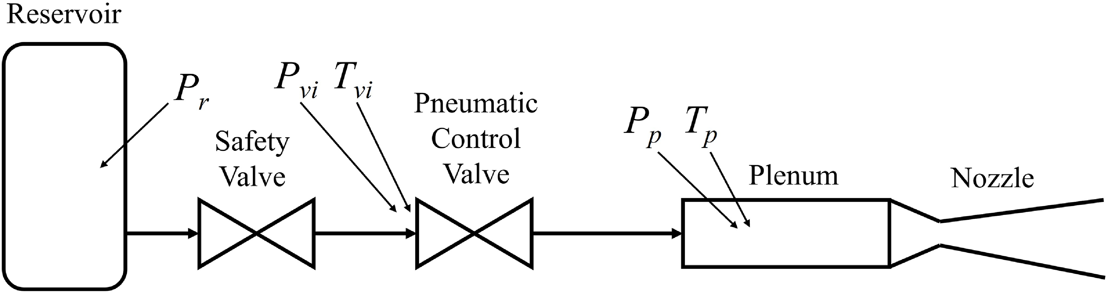
The Missouri S&T Supersonic Wind Tunnel, located in the Aerodynamics Research Laboratory, is a cold-flow, blow-down facility designed for Mach 3 testing. Figure 1 provides a schematic of the setup, which follows the typical layout of blow-down supersonic wind tunnels. The reservoir, where the high pressure gas is accumulated is shown on the left, the air then passes through a control valve (for our case pneumatically operated) that regulates its pressure to the desired level in the plenum chamber. Lastly, it flows through the nozzle. An additional safety valve (on/off), which is manually controlled, isolates the high pressure reservoir when the tunnel is not in use. Downstream, the air flows through the nozzle into the test section, diffuser and exhaust. Since the flow is supersonic, these components do not influence plenum pressure or temperature.
Missouri S&T Supersonic Wind Tunnel diagram. Location of pressure and temperature transducers is shown.

Originally designed in 1968 [Reference Murphy13], the Missouri S&T Supersonic Wind Tunnel was recently upgraded with a new nozzle, test section and diffuser [Reference Gary and Viganò14]. The facility operates with nominal stagnation conditions of 1.52 MPa and 280 K, achieving a Reynolds number per unit length of 1.35 × 10⁸. The main reservoir has a capacity of 7.704 m
 ${{\rm{\;}}^3}$
and pressurises up to 13.8 MPa, enabling test run times of up to one minute. Recent experiments conducted in this facility have confirmed that the nozzle produces a Mach 3 flow with good uniformity in the test section [Reference Gary, McDermott, Worden, Hosder and Viganò15, Reference Roberts and Viganò16].
As mentioned in the introduction, most of the literature on supersonic wind tunnel modeling focused on developing control systems to operate the control valve. Maintaining constant pressure in the plenum, while reducing start-up and shut-down times are critical for the tunnel performance. The Missouri S&T Supersonic Wind Tunnel is currently equipped with a computer-based scheduled-gain PID controller derived from the work of Nott [Reference Nott, Ölçmen, Lewis and Williams17]. This controller is capable of maintaining the plenum pressure within 3% of its nominal value.
Blow-down facilities experience a drop in stagnation (total) temperature due to gas expansion in the reservoir. To mitigate this effect, many facilities employ large thermal masses to raise the gas temperature, such as crushed cans placed within the reservoir [Reference Tucker18]. In our facility, the required thermal mass is instead provided by the long piping connecting the reservoir to the facility, which supplies substantial surface area for heat transfer to the flow during a run.
Figure 1 illustrates the locations of the instruments used in our facility to monitor key operational parameters. Pressure measurements are taken at several critical points: in the reservoir, at the inlet and outlet of the control valve, and within the plenum chamber. Temperature is recorded at both the control valve inlet and the plenum chamber. These data are collected during each test to evaluate the wind tunnel’s performance and ensure optimal operating conditions.
 ${P_r}$
is the pressure in the facility reservoir,
 ${P_{vi}}$
and
 ${T_{vi}}$
are the pressure and temperature at the inlet of the control valve, while
 ${P_p}$
and
 ${T_p}$
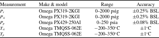
are the pressure and temperature in the plenum. Table 1 lists the sensors used for these measurements.
Facility sensors and their accuracies, as reported by the manufacturers

3.0 Wind Tunnel Model
In this section, we present a new numerical model developed to enhance the understanding of supersonic wind tunnel performance. To clearly explain the impact of each additional modeling step, we will present the model step by step. We begin by replicating the baseline model from the work of Fung et al. [Reference Fung, Settles and Ray1], which will serve as a comparison benchmark. We will then introduce additional modeled effects progressively, starting with heat addition, followed by Joule–Thomson (real gas) effects, and finally pressure losses.
It is important to note that we use our facility to provide data to validate the improved model. However, this model is not specific to our facility and can be easily implemented in other wind tunnels.
3.1 Base model
The baseline wind tunnel model follows the work of Fung et al. [Reference Fung, Settles and Ray1]. We describe the blow-down wind tunnel with two control volumes, one for the reservoir and one for the plenum chamber (see Fig. 1). We then use basic conservation laws to describe the system. Using conservation of mass and energy at both control volumes, we obtain four differential equations:
 \begin{align}\frac{{d{M_r}}}{{dt}} = - {\dot m_v}\end{align}
 \begin{align}\frac{{{M_p}}}{{dt}} = {\dot m_v} - {\dot m_n}\end{align}
 \begin{align}\frac{{d{E_r}}}{{dt}} = - {\dot H_v}\end{align}
 \begin{align}\frac{{d{E_p}}}{{dt}} = {\dot H_v} - {\dot H_n}\end{align}
Equations (1) and (2), which describe mass conservation in the reservoir and plenum respectively, assume that all gas flows from the reservoir into the plenum and then through the nozzle, which is typical for most facilities. If some gas is lost or injected from a separate source (which is not the case for the present facility), the equations must be adjusted accordingly. Equations (3) and (4) describe energy conservation and assume the process is adiabatic, meaning there is no heat transfer between the environment and the gas at either the reservoir or the plenum.
To solve this system of equations, we first need to express the unknowns in terms of thermodynamic variables. The mass in both tanks is represented by the perfect gas law, giving us:
 \begin{align}M = V\rho = \frac{{VP}}{{RT}},\end{align}
where
 $M$
is mass,
 $V$
is volume,
 $P$
is pressure,
 $R$
is the specific gas constant,
 $\rho $
is density and
 $T$
is temperature. Similarly, the internal energy in both volumes can be expressed as:
 \begin{align}E = Me = \frac{{VP{C_v}}}{R},\end{align}
where
 $e$
is the specific energy, and
 ${C_v}$
is the specific heat at constant volume.
The mass flows in Equations (1) and (2) also need to be expressed in terms of thermodynamic variables. In this work, we assume that the nozzle is always choked. While this assumption does not hold at the start and end of a test, it is reasonable given that these intervals are relatively short and that the nozzle can achieve choking at comparatively low pressures, a scenario commonly encountered in the literature. With this assumption:
 \begin{align}{\dot m_n} = {A_n}\frac{{{P_p}}}{{\sqrt {{T_p}} }}\sqrt {\frac{\gamma }{R}} {\left( {\frac{2}{{\gamma + 1}}} \right)^{\frac{{\gamma + 1}}{{2\left( {\gamma - 1} \right)}}}}\end{align}
A choked nozzle is a common approach in literature [Reference Hwang and Hsu2], however, different methods are employed for modeling the flow through the control valve. In our facility, where the reservoir pressure is significantly higher than the target plenum pressure, the control valve also operates in a choked condition during normal operations. We can then express the mass flow through the valve as a function of the total pressure and temperature at the valve inlet. The important distinction is that, while the nozzle throat area is fixed (at least in our facility), the control valve throat area varies continuously. For our control valve, we determined the throat area as a function of the percentage valve opening using tables provided by the manufacturer.
Substituting these expressions into Equations (1)–(4) we obtain a system of four differential equations with four unknowns; plenum total pressure and temperature, and reservoir total pressure and temperature. The equations can then be solved through a numerical solver.
However, the system has an additional unknown through the valve area (or equivalently, the valve opening percentage). In general, this can be resolved in one of two ways: either by introducing additional equations to compute the valve area as part of a control strategy, as is commonly done in the literature to regulate plenum pressure (e.g. via a PID controller), or by prescribing the valve area directly as an input to the model. Because the objective of the present work is to develop and validate a new model, rather than a new controller, the latter approach is adopted. Accordingly, the valve opening is specified as a function of time, using measurements recorded during each experimental run.
In deriving this system, we have made a series of assumptions. We assume that the flow is adiabatic throughout the system and that there are no pressure losses, except in the control valve. Additionally, we have neglected the dynamics of the piping that connects the reservoir to the plenum. This leads us to conclude that the mass exiting the reservoir is identical to the mass entering the valve. Therefore, in Equation (1), we used
 ${\dot m_v}$
rather than
 ${\dot m_r}$
.
It is important to note that in our facility, the control valve is positioned right before the plenum, with the majority of the piping running from the reservoir to the valve – a typical configuration. Lastly, we assume that the working gas, which is typically air, behaves as a perfect gas.
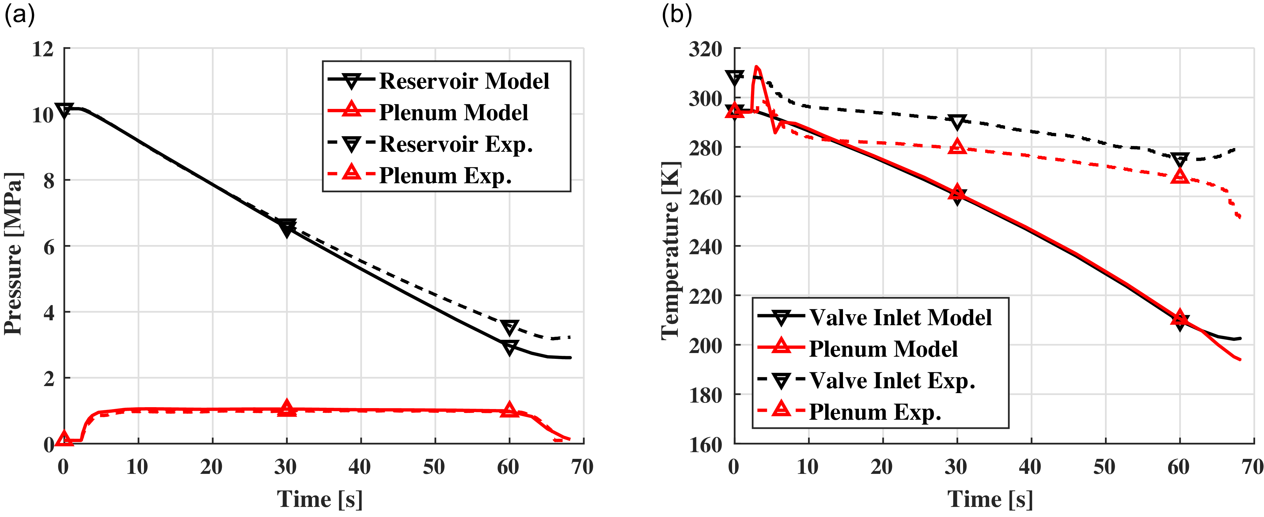
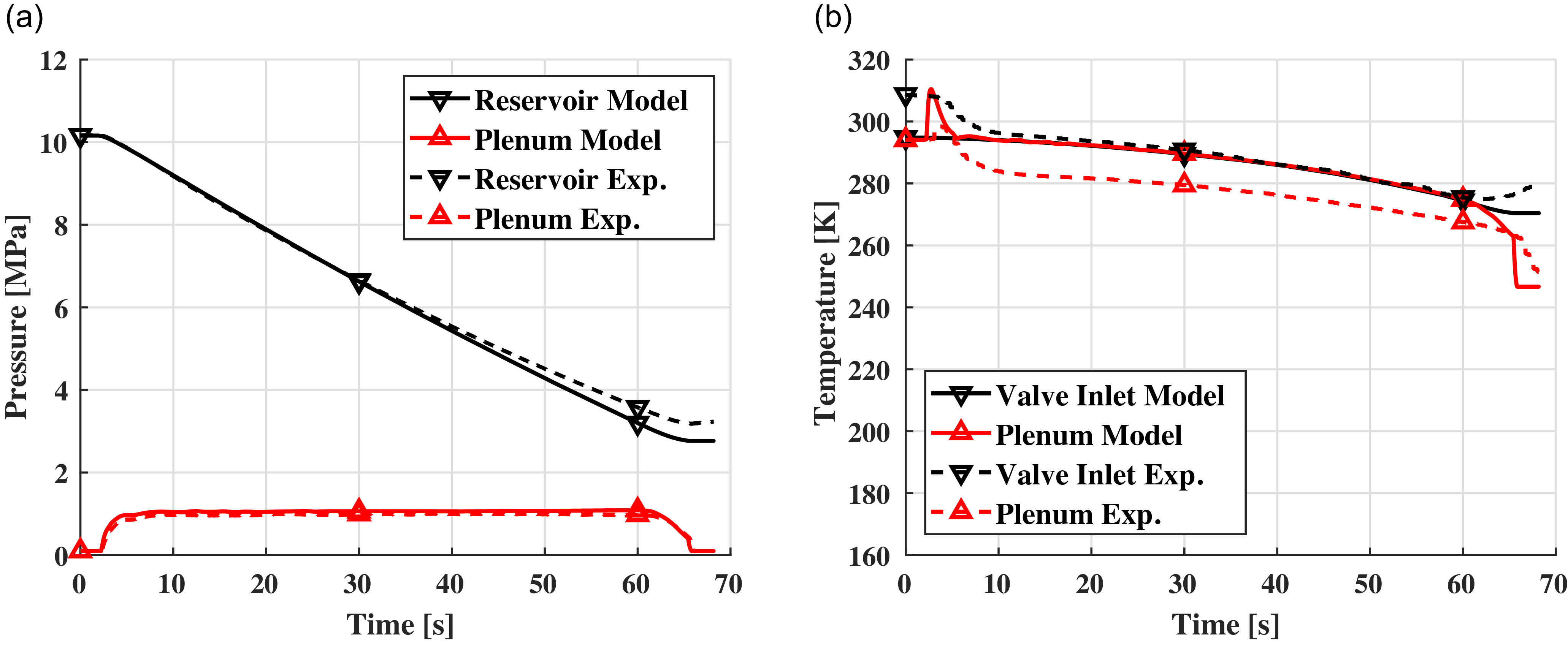
Figure 2 shows a comparison of this base model with experimental data from a supersonic tunnel test run. Figure 2(a) compares the pressures predicted by the model with experimental measurements for both reservoir and plenum. The model’s plenum pressure compares well with the experimental measurements, with an average error of 5% for this particular test. Since most literature works were interested in the plenum pressure, it is then clear why the base model from Fung et al. [Reference Fung, Settles and Ray1] and the similar successive ones were deemed sufficient. However, Fig. 2(b) shows a different trend for temperatures. The adiabatic assumption leads to temperatures significantly lower than reality with a 34% error towards the end of the test. Additionally, the base model fails the capture the initial temperature drop observed in experimental data, which is due to Joule–Thomson effect. The error in temperature is reflected in the reservoir pressure in Fig. 2(a). Since mass flow out of the reservoir scales with
 $1/\sqrt T $
(Equation (7)), the model over-predicts the mass flow exiting the reservoir and thus its pressure decreases faster than reality. An interesting feature in Fig. 2(b) is the spike in plenum temperature at the beginning of a test. The sharp temperature increase is seen in both simulation and experimental measurements and it is due to the initial compression of the air [Reference Leavy19]. Lower values in the experimental case can be attributed to the thermal mass of the plenum (including flow spreader and screens).
Comparison between base model and experimental data. (a) Pressures, (b) Temperatures.

The results in Fig. 2 show that the experimental temperature is not correctly captured by the base model. Two major differences are visible in the actual measured data. First, the process is diabatic since temperature remains significantly higher in both the valve inlet and the plenum, and second a sharp drop in plenum temperature is visible at the beginning of a test. These observations motivate the inclusion of non-ideal effects, which are introduced and discussed in the following section.
3.2 Heat addition
The primary driver of the diabatic process is the thermal mass of the tanks and pipes that make up the system. As the working gas expands and cools, it removes heat from the (mainly) steel. This is true in all parts of the wind tunnel, the reservoir, the piping, the plenum, nozzle, etc. However it is more severe in some parts than others. In our facility, heat addition is assumed to occur upstream of the control valve, primarily in the long piping connecting the reservoir to the valve, while heat transfer from the reservoir tanks is implicitly captured by the energy balance. This assumption is motivated by the forced-convection nature of the heat transfer process: although the flow remains well within the subsonic regime, gas velocities are higher in the piping than in the reservoir or plenum due to the smaller diameter.
Three observations corroborate this hypothesis. First, Fig. 2(b) shows there is little difference (maximum 7%) between trends in the temperature at the control valve inlet and in that in the plenum. This indicates that the heat transfer in the plenum is small and can be considered adiabatic. Second, observations during multiple experiments showed that the pipes were significantly colder than the reservoir or plenum at the end of a test, pointing to a much more significant heat removal. Third, a predictive version of the model, presented later, relies exclusively on the thermal mass of the piping and does not use experimental temperature data; despite this, it shows good agreement with measured results, further supporting the assumption that the dominant heat transfer occurs in the piping.
To model the heat addition we first rely on experimental data. The temperature at the valve inlet
 ${T_{vi}}$
is recorded during each test. We can then define
 ${\rm{\Delta }}T = {T_{vi}} - {T_{va}}$
, where
 ${T_{va}}$
is the valve inlet temperature under adiabatic conditions.
 ${\rm{\Delta }}T$
then is the temperature difference between adiabatic and diabatic expansions. If we assume a quasi-steady process, we can then express the instantaneous thermal power added in the pipes as:
 \begin{align}\dot q\left( t \right) = {\dot m_v}{\rm{\Delta }}h\left( t \right)\end{align}
where the specific enthalpy, for a perfect gas, is calculated as
 ${\rm{\Delta }}h\left( t \right) = {C_p}{\rm{\Delta }}T\left( t \right)$
. The issue with this approach is that each test has a different function of
 $\dot q\left( t \right)$
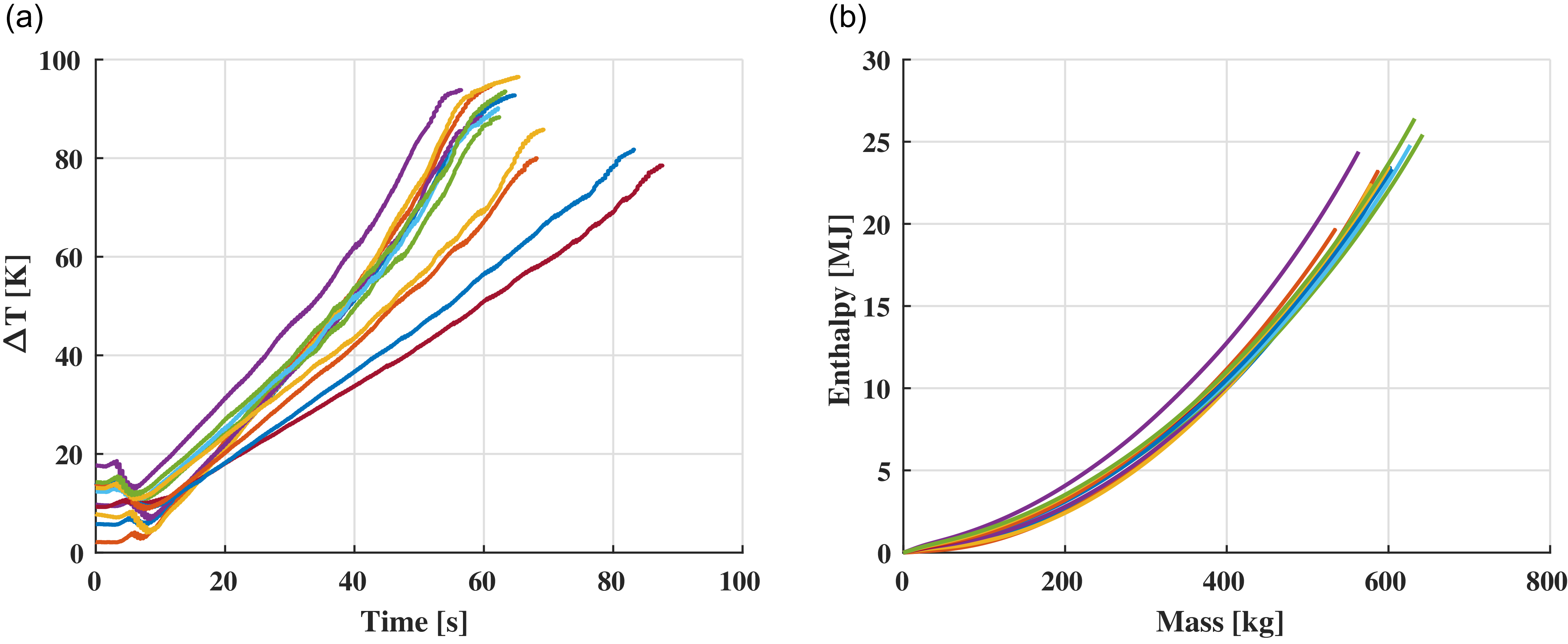
, thus not allowing the model to predict future experiments. This is shown by the different curves in Fig. 3(a). This figure shows the temperature difference for 12 wind tunnel tests. These tests were performed at different plenum pressure settings (thus with different mass flow rates). The large scattering of temperature differences at time equal 0 is due to the fact that while most of the piping is indoor (and thus at an almost constant temperature throughout the year), the reservoir is outdoor and so its temperature changes seasonally and daily based on sun exposure.
(a) Temperature difference vs time, and (b) total energy vs mass.

An alternative approach is to express the integral enthalpy (Equation (9)) as a function of the integral mass (Equation (10)) through the control valve. The integral mass is independent of the specific testing parameters and as such is more generally applicable. Similarly, we hypothesised that the energy extracted from the piping should be a function of the mass of gas processed. Figure 3(b) shows the integral enthalpy against the integral mass for the same 12 tests from Fig. 3(a). In this case the data collapse on a quadratic curve. Since this curve is not function of the specific testing conditions, we can now use it in our model to predict heat addition.
 \begin{align}{H_I}\left( t \right) = \mathop \smallint \nolimits_0^t {\dot m_v}{\rm{\Delta }}hdt\end{align}
 \begin{align}{M_{vI}}\left( t \right) = \mathop \smallint \nolimits_0^t {\dot m_v}dt\end{align}
To do this, we use the data in Fig. 3(b) to extract a best fit polynomial curve. For this model we selected to express the enthalpy as
 ${H_I} = BM_{vI}^2$
, where B is a coefficient. The y-intercept is zero by definition. The linear term was also imposed as zero (it will shortly be explained why). The coefficient B is then calculated from a best fit of the existing data. For the values in Fig. 3(b), the resulting curve has a
 ${R^2} = 0.9648$
, showing a good approximation.
 \begin{align}\frac{{d{H_I}}}{{d{M_{vI}}}} = {\rm{\Delta }}h\end{align}
 \begin{align}{\rm{\Delta }}T = \frac{{2B{M_{vI}}}}{{{C_p}}}\end{align}
In order to use this expression, we can take the derivative of the total enthalpy with respect to the mass, as shown in Equation (11). Doing the same with the polynomial expression, we can finally express the change in temperature as a linear function of the integral mass as shown in Equation (12). The last equation shows why the linear term in the polynomial approximation was set to zero, so that at 0 mass, there is no heat addition. Note that, while Equation (12) can now be used to predict the effects of heat addition, the coefficient
 $B$
is facility-specific and requires experimental data to be calculated.
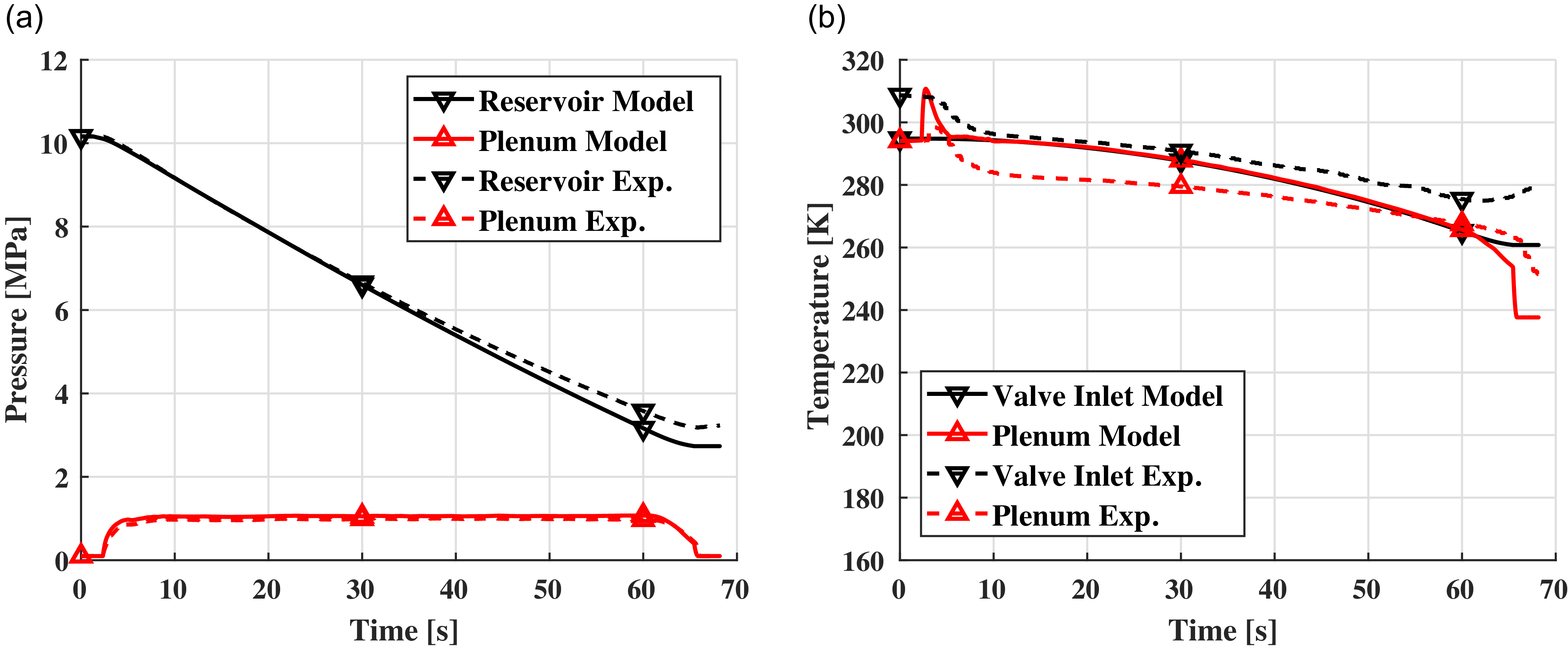
Finally, by adding Equation (12) to the model, we can now calculate the correct valve inlet temperature (since the mass flowrate through the valve is already calculated, it is easy to obtain the integral mass). Figure 4 shows the comparison between the model with heat addition and the same experimental data from Fig. 2. The pressure plot (Fig. 4(a)) shows little difference from the base model, with only the reservoir pressure prediction improving. However, the temperature plot (Fig. 4(b)) now shows a very good match between the simulated and the measured valve inlet temperatures. The plenum temperature prediction also improved, albeit it is now over-predicted. The reason (and the solution) for this is in the following section.
Comparison between base model with heat addition and experimental data. (a) Pressures, (b) Temperatures.

The experimental cases used to determine the heat-addition coefficient
 $B$
span the full operational total-pressure range of the facility, as illustrated by the 12 tunnel runs presented in this study. The good agreement observed across these conditions indicates that the proposed heat-addition model remains applicable over a wide range of operating pressures. It is noted, however, that the coefficient
 $B$
is facility-specific, as it represents the combined heat-transfer characteristics of a given tunnel configuration, including geometry, materials and convective environment; nevertheless, the methodology used to model heat addition and to determine
 $B$
from experimental data is general and may be applied to other blow-down facilities, and in the present case a limited number of experimental runs (12) was sufficient to determine it. Finally, while the present facility is characterised by a large thermal mass upstream of the control valve, the same modeling approach may be extended to facilities with significant piping downstream of the valve by introducing an additional energy balance describing the temperature evolution between the valve and the plenum, along with a second heat-addition coefficient (e.g.
 ${B_2}$
), without altering the underlying modeling framework.
One issue remains with the presented solution for heat addition, it requires experimental measurements to obtain the coefficient B, as such it can’t be used in the design phase of a new facility. However, a physical explanation of the process can be provided. The model assumes that the heat is removed from the pipes connecting the reservoir to the control valve. Since the length of these pipes is known (and could be estimated during the design phase), as well as their mass per unit length, we can calculate their thermal mass. We assume that the pipes do not exchange heat with the surrounding, such that heat is exchanged only between pipes and internal gas. This is a reasonable assumption since the forced convection inside the pipe is considerably larger than the natural convection between the pipes and environment. We can also assume that, since the convective heat transfer is large and the wall thickness of the pipes is not large, the pipes are at the same temperature of the gas. We can then express the valve inlet temperature as:
 \begin{align}\frac{{d{T_{vi}}}}{{dt}} = \frac{{{{\dot m}_v}{C_p}\left( {{T_r} - {T_{vi}}} \right)}}{{{M_{pipes}}{C_{pipes}}}}\end{align}
where
 ${M_{pipes}}$
and
 ${C_{pipes}}$
denote the mass and specific heat of the pipes, respectively. Results from implementing Equation (13) into the base model are shown in Fig. 5. The pressure plots (Fig. 5(a)) show minimal variation relative to experimental pressure traces. The valve inlet temperature prediction in Fig. 5(b) initially aligns with experimental data but gradually deviates, reaching a difference of approximately 10 K by the end of the run. These results were obtained without relying on any experimental data. Consequently, both approaches have distinct merits: Equation (13) is suited for the design phase, whereas Equation (12) yields more accurate predictions once experimental data are available. For the remainder of the manuscript Equation (12) will be used. It is important to note that, while in our facility the thermal mass is provided by the long piping system, other facilities may incorporate thermal mass directly within the reservoir or in a dedicated thermal mass tank [8]. In such cases, Equation (13) remains applicable, with
 ${M_{pipes}}$
and
 ${C_{pipes}}$
replaced by the corresponding properties of the respective thermal masses.
Comparison between base model with predicted heat addition and experimental data. (a) Pressures, (b) Temperatures.

3.3 Joule–Thomson effect
The Joule–Thomson effect is a real gas effect where total temperature is not conserved in an isenthalpic process. The consequence is that when a gas is expanded, we can observe a change in temperature. Although air is typically considered a perfect gas, large pressure changes, such as those occurring when throttling through a control valve, can make the Joule–Thomson effect significant. For temperatures and pressure ratios typically encountered in supersonic wind tunnels, the Joule–Thomson effect decreases the total temperature after the control valve. Joule–Thomson is a well-documented phenomenon in wind tunnel design literature [Reference Pope and Goin8–Reference Lukasiewicz11].
The Joule–Thomson effect is more significant for larger pressure ratios. Thus, for blow-down wind tunnels, it is most severe at the beginning of a test, when the reservoir pressure is at its maximum, and decreases as the reservoir pressure drops. This trend is opposite to that of gas cooling due to expansion in the reservoir, which becomes more pronounced as the reservoir pressure approaches its minimum. Consequently, while the Joule–Thomson effect causes an initial temperature drop across the valve, it mitigates plenum temperature drift toward the end of a test and helps maintain a more constant temperature overall.
Figure 2(b) shows the presence of the Joule–Thomson effect in our facility. We can observe a drop in temperature between the valve inlet and the plenum temperatures. This drop is highest at the beginning of the test and slowly decreases as the reservoir pressure drops. On the other hand, the present numerical model predicts that valve inlet and plenum temperature are approximately the same during the whole test, which will now be addressed.
To model the Joule–Thomson effect and real gas effects in general, we replace the calculation of energy and enthalpy in the model. Up to now, under the assumption of a calorically perfect gas, energy and enthalpy were calculated using constant specific heats. Instead, we now use real gas tables from the work of Lemmon et al. [Reference Lemmon, Jacobsen, Penoncello and Friend20], for which enthalpy (or energy) is expressed as
 $h = f\left( {P,T} \right)$
. Importantly, since Equations (1)–(4) are expressed in terms of energy and enthalpy, the original model remains valid; only the calculation of energy and enthalpy has changed.
3.3.1 Heat addition for real gases
In the previous section, we discussed heat addition effects for a calorically perfect gas, although real gas effects also influence this process. Equations (9) and (11) are written in terms of enthalpy, so they remain valid. Similarly to the previous section, we then modify the calculation of enthalpy. Instead of using
 ${\rm{\Delta }}h\left( t \right) = {C_p}{\rm{\Delta }}T\left( t \right)$
for a calorically perfect gas, we now calculate enthalpy from real gas tables [Reference Lemmon, Jacobsen, Penoncello and Friend20]. It is therefore more convenient to re-express Equation (12) in terms of enthalpy rather than temperature:
 \begin{align}{\rm{\Delta }}h = 2B{M_{vI}}\end{align}
Equation (14) provides the change in enthalpy due to heat addition. However, using the same methods previously discussed, the coefficient B must now be determined from experimental data using real gas tables to calculate enthalpy. The results obtained with real gas considerations collapse again onto a parabolic curve like in Fig. 3(b). However, they now yield an improved correlation coefficient of
 ${R^2} = 0.9903$
. Thus, incorporating real gas effects improves the accuracy of heat addition predictions.
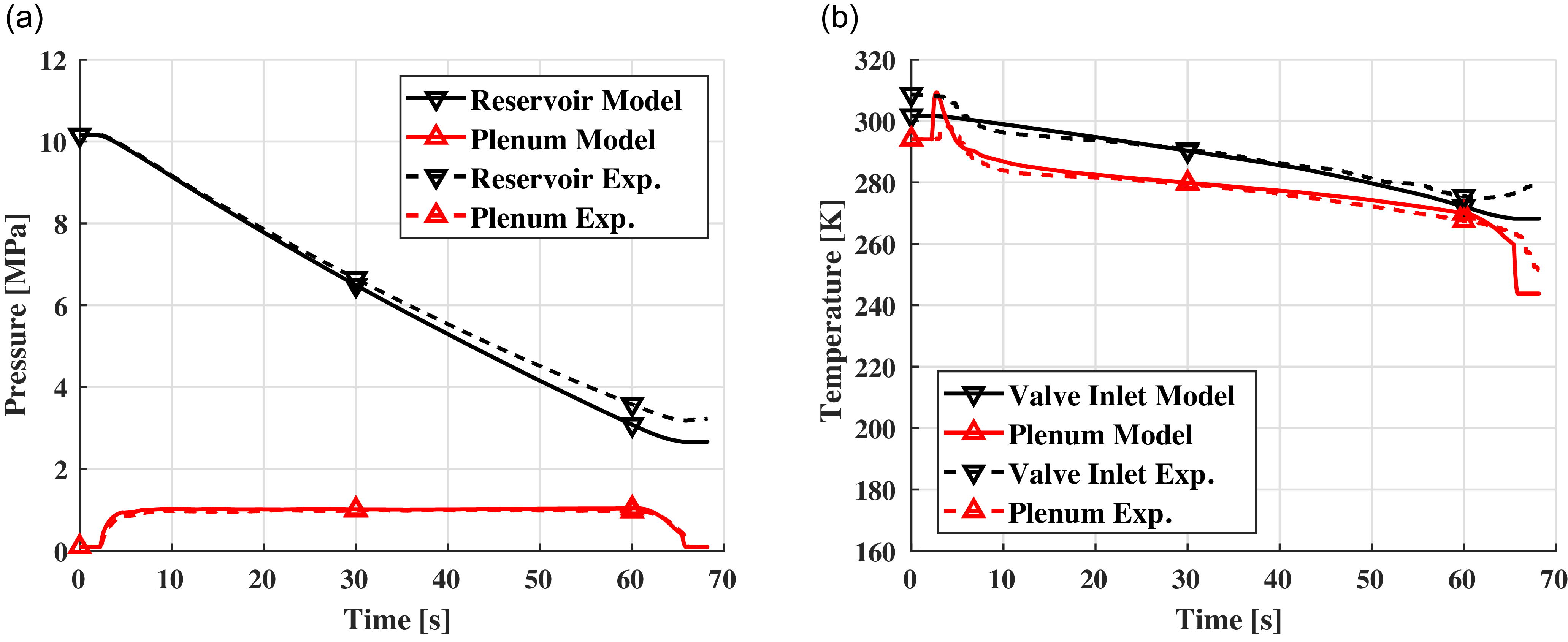
Figure 6 shows the results for the model with real gas effects. Once again, pressure plots in Fig. 6(a) are not affected significantly. However, Fig. 6(b) now shows a much better agreement on the plenum temperature. The drop observed from the experiments is now replicated by the model. It is important to note that real gas effects do not require any previous experimental data to be modeled and thus can be implemented in the design phase.
Comparison between model with heat addition and Joule–Thomson effect and experimental data. (a) Pressures, (b) Temperatures.

3.4 Pressure losses
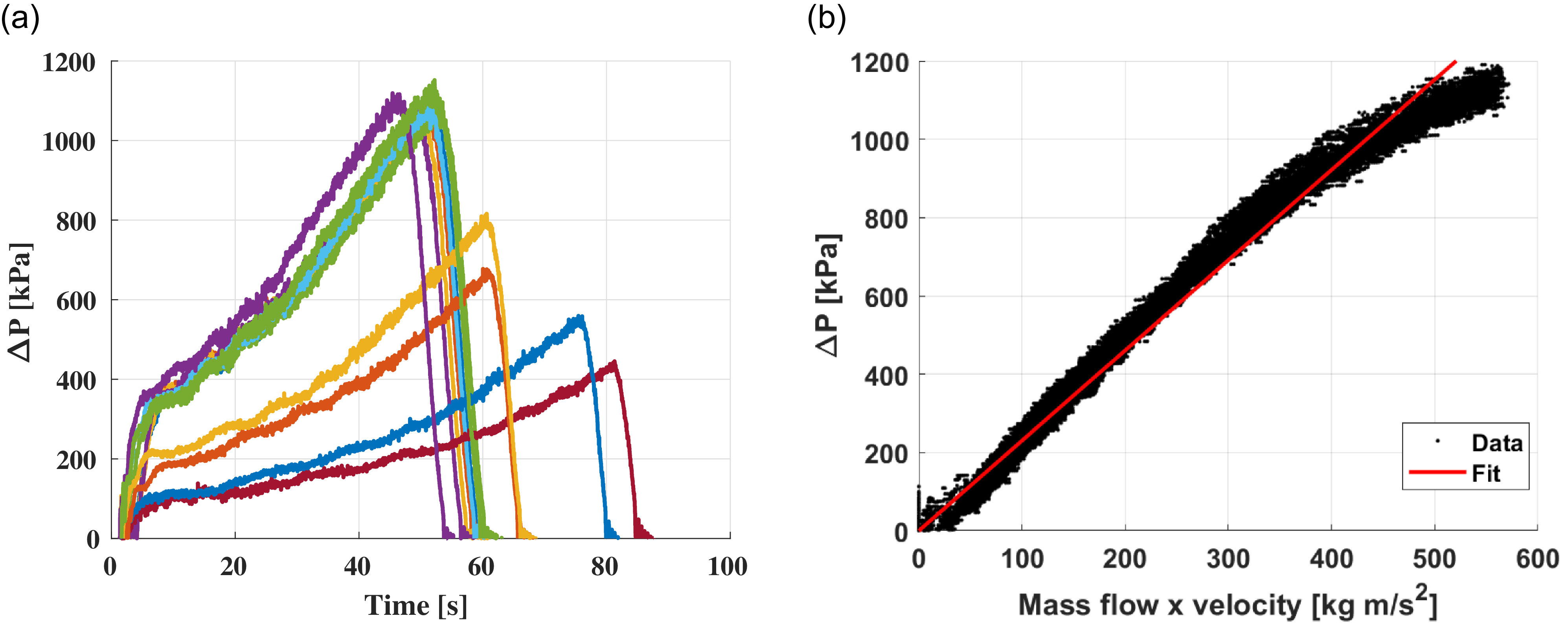
The last effect we are going to add to the base model is not about temperature, but rather pressure. Figure 7(a) shows the measured total pressure difference between the reservoir and the valve inlet versus time. This figure shows that the pressure losses in the piping system can be significant. For high plenum pressure testing, which means larger mass flow rates (and thus velocities) through the pipes, pressure losses can exceed 1 MPa, which is on the same order of magnitude of the target plenum pressure. Thus, pressure losses should be included in the wind tunnel model.
(a) Measured pressure losses vs time. Each colour represents a different experiment. (b) Pressure losses vs mass flow times velocity.

In the current model we have assumed that the pressure at the control valve inlet is equal to that in the reservoir (
 ${P_{vi}} = {P_r}$
), we are now going to derive a model that calculates the pressure at the valve based on losses in the pipes. The flow in the piping system can be considered quasi-steady, and due to the low speed involved, incompressible. We can then use Darcy-Weisbach equation to model the pressure losses in the system.
 \begin{align}{\rm{\Delta }}P = f\frac{L}{D}2\rho {v^2}\end{align}
By replacing density using continuity, and expressing in term of valve inlet pressure, we obtain:
 \begin{align}{\rm{\Delta }}P = {P_r} - {P_{vi}} = 2f\frac{L}{{DA}}\dot mv\end{align}
In Equation (16)
 $L$
,
 $D$
and
 $A$
are the length, diameter and cross-sectional area of the pipes. The friction factor
 $f$
is normally a function of the Reynolds number, however, since this is in the
 ${10^7}$
range, the friction factor is a constant [Reference Moody21]. Minor losses associated with fittings and geometric changes have the same functional dependence on velocity and are therefore implicitly captured within the pressure-loss formulation adopted here. We then expect a linear relation between the pressure losses and the product of mass flow and velocity. Figure 7(b) shows the measured pressure loss (from the same 12 tests of Fig. 7(a)) vs mass flow times velocity (
 $\dot mu$
) as well as a linear best fit. Although experimental measurements depart slightly from linearity at higher mass flowrates, the data fit well with the linear approximation with an
 ${R^2} = 0.9804$
. This shows that the pressure difference is due to frictional losses in the pipes. Equation (16) can then be added to the model to predict pressure losses in the pipes.
We can then calculate the pressure at the valve inlet from the reservoir pressure minus the pressure loss. This adds one algebraic equation to the model. Figure 8 shows the results from this model, which now includes head addition, Joule–Thomson and pressure losses. The temperature plots in Fig. 8(b) do not change significantly. However, Fig. 8(a) shows an improved agreement between all pressures. Note that the valve inlet pressure is now also plotted, it was omitted before since the model assumed it to be identical to the reservoir pressure.
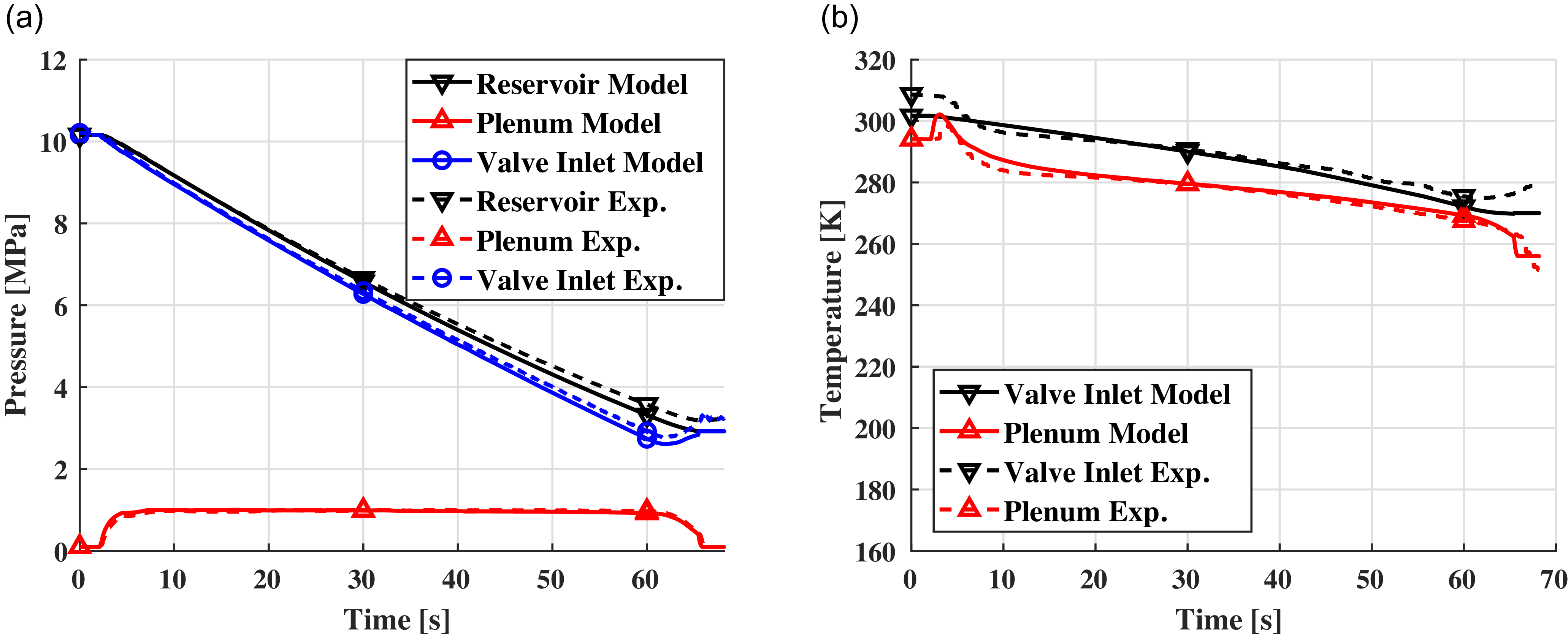
Comparison between model with heat addition, Joule–Thomson effect, and pressure losses and experimental data. (a) Pressures, (b) Temperatures.

4. Comparison With Experimental Data
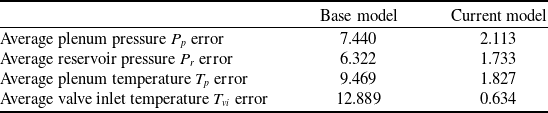
In this section, we evaluate how well our model predicts experimental data beyond the specific case previously presented. We ran the model against the same 12 experimental tests shown in Fig. 3(a) and calculated the instantaneous errors in both pressure and temperature. To analyse the model’s performance, we averaged the error profiles for instances when the plenum pressure was within 90% of its target value. This procedure allows to focus on the steady state portion of each wind tunnel run, the part where scientific measurements in the test section are performed. This averaging process was conducted for both the base model and the improved model we have presented.
Table 2 shows the average error results for both the base and current models. The most significant improvement is observed in the temperature modeling; both the plenum and valve inlet temperatures are now within 2% of the experimental data. In contrast, the base model exhibited average errors between 9% and 13%. However, due to the incorrect treatment of temperature drift, the maximum error could exceed 35% towards the end of a test run as shown in Fig. 2(b), an issue that is resolved in the present model through the inclusion of heat-addition effects.
Comparison of average model error between base [Reference Fung, Settles and Ray1] and current models

Improved prediction of the temperature profile in the plenum is crucial for several reasons. Blow-down wind tunnels are inevitably affected by thermal drift, which means that both the Reynolds number and velocity in the test section are not constant. Large thermal drifts also affect the nozzle boundary layer thickness, which slightly alters the Mach number. Thus, accurately predicting thermal drift can inform the design phase and help devise strategies to mitigate its effects.
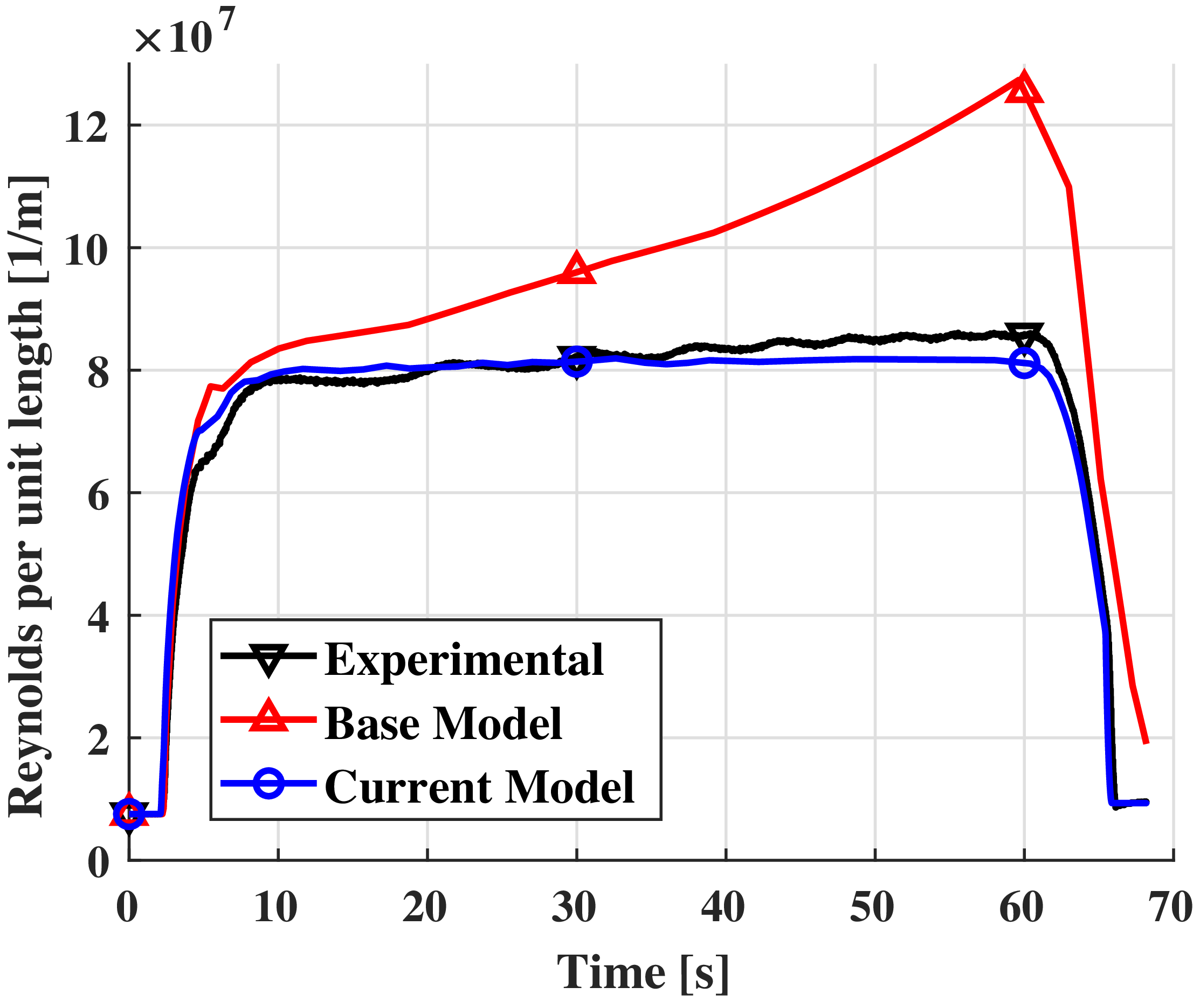
Figure 9 illustrates the effect of model choice on the predicted test section Reynolds number (per unit length). The base model, which neglects heat addition, deviates from the experimental data almost immediately, with the error growing over time to a maximum of 48% by the end of the test. In contrast, the current model closely matches the experimental data, with a maximum error of only 6%, just one-eighth of the error produced by the base model. Similar trends are observed across the full range of operating conditions, with the base-model Reynolds-number error increasing from approximately 34% at the lowest pressure setting to over 70% at the highest, while the present model remains within approximately 6% for all test conditions.
Comparison of test section Reynolds number predictions vs experimental data.

Table 2 shows that the modeling of pressures has also improved, albeit to a lesser extent. With both plenum and reservoir pressures now within 2% of the experimental measurements, the error is reduced to one-third of that observed in the base model. Improved predictions of plenum pressure are particularly valuable for the development of valve control systems. As discussed in the introduction, most models of supersonic wind tunnels have been developed for designing and refining control algorithms for the pressure-regulating valve. Our model can now more accurately predict not only the plenum pressure but also the reservoir and valve inlet pressures, thereby facilitating better training for control algorithm design.
5.0 Conclusion
In this study, we presented an improved numerical model for a supersonic wind tunnel that incorporates essential thermal effects, enhancing the accuracy of temperature and pressure predictions. By systematically building upon the baseline model established by Fung et al. [Reference Fung, Settles and Ray1], we introduced critical factors such as heat addition, real gas effects and pressure losses in the piping system.
Our results demonstrate that the improved model significantly enhances the fidelity of temperature predictions, bringing them within 2% of experimental measurements, compared to the base model’s errors of 9% to 13%. Additionally, we achieved a marked reduction in pressure prediction errors, facilitating more reliable modeling for the design and development of control algorithms for pressure-regulating valves.
The advancements presented here are essential for improving the operation and accuracy of supersonic wind tunnels. By accurately predicting temperature variations, our model enables more precise calculations of velocity and Reynolds number during testing, which are critical for reliable and repeatable experimental outcomes. Additionally, the enhanced pressure prediction, achieved by accounting for heat addition, Joule–Thomson effects and pressure losses, allows for a more accurate assessment of plenum, reservoir and valve inlet pressures. These refinements directly support the design of more effective and precise control systems capable of responding accurately to the dynamic conditions encountered during operation.
In sum, this model contributes to higher-quality testing by reducing temperature and pressure discrepancies, thereby improving test consistency and reliability. With these improvements, researchers and engineers can achieve more precise control over flow conditions, enhancing the overall effectiveness of supersonic wind tunnel experiments in high-speed aerodynamics research.
Competing interests
The authors declare none.