1. Introduction
Understanding the stability of liquid layers with holes is of fundamental importance for numerous applications, such as coating, micropatterning and lithography (Schäffer et al. Reference Schäffer, Harkema, Roerdink, Blossey and Steiner2003; Weinstein & Ruschak Reference Weinstein and Ruschak2004; Kumar Reference Kumar2015; Lee et al. Reference Lee, Brun, Marthelot, Balestra, Gallaire and Reis2016; Lohse Reference Lohse2018). Coating processes aim to produce uniform thin films on the underlying solid substrate, but under certain conditions, holes can form in the film. While some of these holes may disappear naturally, others can persist as undesirable defects. Moreover, micropatterning through dewetting has been employed to create desired features in a wide range of solid materials, including metallic thin films (Ferrer, Halajko & Amatucci Reference Ferrer, Halajko and Amatucci2014) and soft rubber substrates (Martin, Buguin & Brochard-Wyart Reference Martin, Buguin and Brochard-Wyart2001). To further apply and expand this approach, a comprehensive understanding of the statics and dynamics of thin liquid films with holes is necessary. Immersion lithography, a technique that involves lithography under a water film (with a refractive index of 1.33, rather than 1.00 for air) between the optical lens and the wafer, the resolution of lithography can be improved by using a larger numerical aperture. However, the presence of a hole in the liquid film, acting as a defect, can significantly impact the quality of the final products. Furthermore, the hole may collapse and introduce bubbles in the liquid film. Considering its importance, the wetting behaviour of a hole in a liquid layer has attracted considerable attention over the past decades.
The pioneering studies of Lamb (Reference Lamb1916) and Padday (Reference Padday1971) explored equilibrium solutions for liquid–vapour systems with axisymmetric profiles in their comprehensive works. Taylor & Michael (Reference Taylor and Michael1973) conducted experimental and theoretical investigations on axisymmetric holes in liquid layers. They discovered that, for an infinitely extended film, the equilibrium solution of the liquid–vapour interface is energetically unstable. Furthermore, they demonstrated that this equilibrium solution serves as a criterion to determine the stability of a hole (whether it remains open or closes), which was verified through experiments on holes in a mercury layer. However, experiments on a hole in a water layer on paraffin wax (which exhibits moderate hydrophobicity) did not provide a clear distinction regarding whether the hole would remain open or close. In addition, they observed that holes of various sizes could remain stationary due to contact angle hysteresis. Sharma & Ruckenstein (Reference Sharma and Ruckenstein1990) conducted theoretical studies on the equilibrium and stability of holes in liquid layers using energy criteria. Their findings revealed the existence of two equilibrium solutions for holes with a certain contact angle, where the hole with the larger radius is unconditionally stable and the one with the smaller radius is unstable. Their analyses suggested that, in practice, if the radius of the hole exceeds a critical value, the hole will remain open; otherwise, it will close. Moriarty & Schwartz (Reference Moriarty and Schwartz1993) employed a lubrication model to investigate the stability and evolution of axisymmetric holes in thin liquid layers bounded within a finite domain. Their numerical solution considered the motion of the contact line at the edge of the hole and contact angle hysteresis. They found that a hole slightly larger than the critical value for opening can dynamically close due to the influences of contact angles. Wilson & Duffy (Reference Wilson and Duffy1996) employed an asymptotic analysis to examine the equilibrium of axisymmetric holes in thin liquid layers. Their study focused on infinitely extended liquid layers, considering the effects of gravity and surface tension. López, Miksis & Bankoff (Reference López, Miksis and Bankoff2001) conducted a theoretical study on the motion of a thin viscous layer of fluid on a horizontal solid surface bounded laterally by a hole and a vertical solid wall. By employing linear stability analysis, they found that equilibrium solutions with small holes are unstable to axisymmetric disturbances for a container of fixed diameter, while large holes become unstable to non-axisymmetric disturbances. Zheng et al. (Reference Zheng, Fontelos, Shin, Dallaston, Tseluiko, Kalliadasis and Stone2018a,Reference Zheng, Fontelos, Shin and Stoneb) investigated the dynamics of a healing film driven by surface tension, deriving a self-similar solution to describe the dynamics of the film's profile by employing the lubrication model. Lv, Eigenbrod & Hardt (Reference Lv, Eigenbrod and Hardt2018) conducted experimental and theoretical studies on the stability and dynamics of holes in bounded liquid layers. They demonstrated that, for liquid layers with thicknesses of the order of the capillary length, stable holes exist when the hole diameter exceeds a critical value  $d_c$. Beyond this stability threshold, the hole collapses. They also found that
 $d_c$ increases with the size of the container, while its dependence on the contact angle is weak. Ni et al. (Reference Ni, Chu, Li, Luo and Wen2021) investigated the behaviours of impact-induced holes on superhydrophobic surfaces. They found that the holes primarily exhibit growth, stability or collapse depending on their initial size, with the dynamics of the hole resulting from the interplay between capillary force and hydrostatic pressure.
In addition to the above studies that mainly focused on the equilibrium solution and stability of the liquid–vapour interface, research on the dynamic closure of holes has also been conducted, both experimentally and theoretically. Gratton & Minotti (Reference Gratton and Minotti1990) developed a theoretical model based on lubrication theory to investigate the spreading of viscous gravity currents over a rigid surface. They obtained a self-similar solution of the second kind, describing the axisymmetric collapse of a viscous fluid towards the origin within a finite domain. Diez, Gratton & Gratton (Reference Diez, Gratton and Gratton1992) conducted theoretical and experimental investigations on the axisymmetric flow of highly viscous fluids towards a central orifice. The flow in this scenario is governed by a balance between gravity and viscous forces, with surface tension effects assumed to be small. They derived a self-similar solution that matched well with experimental results when the hole radius became sufficiently small compared with its initial radius. Dijksman et al. (Reference Dijksman, Mukhopadhyay, Gaebler, Witelski and Behringer2015) investigated the dynamics of hole collapse in a liquid film experimentally and theoretically, focusing on converging fluid films driven by both surface tension and gravitational forcing. In contrast to the findings of Diez et al. (Reference Diez, Gratton and Gratton1992), Dijksman et al. (Reference Dijksman, Mukhopadhyay, Gaebler, Witelski and Behringer2015) also considered situations where surface tension plays a dominant role in the spreading dynamics of the flow in the liquid. Bostwick, Dijksman & Shearer (Reference Bostwick, Dijksman and Shearer2017) investigated the collapse dynamics of an axisymmetric hole in a thin film that wets the bottom of a rotating container with vertical sidewalls, employing a lubrication theory. Their model accounted for the effects of surface tension, gravity and the centrifugal force. They reported power-law forms for the collapse time in limits where the capillary force and gravitational force played dominant roles. Zheng et al. (Reference Zheng, Fontelos, Shin, Dallaston, Tseluiko, Kalliadasis and Stone2018a) conducted theoretical and experimental investigations and presented a self-similar solution of the liquid–vapour profile of a hole in a spreading liquid film. Bankoff et al. (Reference Bankoff, Johnson, Miksis, Schluter and Lopez2003) explored the dynamics of a hole in a thin viscous film on a horizontal surface through experimental and theoretical studies. They observed three different behaviours of the hole, influenced by the initial film thickness and the diameter of the container. Factors such as hole diameter, front velocity, dynamic contact angle and liquid–vapour interface related to the shrinking of the hole were investigated. Their findings indicated that the final hole diameter increases as the initial fluid depth decreases. Lv et al. (Reference Lv, Eigenbrod and Hardt2018) investigated the dynamics of the hole and the evolution of the liquid film profile after collapse. They identified distinct power-law relationships for the diameter of the collapsing hole and the minimum thickness of the liquid film shortly after collapse. Lu & Corvalan (Reference Lu and Corvalan2019) recently studied the dynamics of a non-axisymmetric hole undergoing capillary collapse in a liquid sheet with small dynamic viscosity, using scaling arguments and high-fidelity simulations. For low-viscosity fluids, they found two distinct dynamical regimes: an initial inviscid regime and a final Stokes regime. The authors demonstrated that the cross-over hole radii, marking transitions between these two regimes, follow power-law relations with fluid viscosity. Furthermore, Lu et al. (Reference Lu, Ferri, Ubal, Campanella and Corvalan2019) employed scaling arguments supported by high-fidelity simulations to investigate the dynamics of a non-axisymmetric hole in a high shear-thinning liquid sheet. They discovered that shear-thinning effects accelerate the collapse of the hole by reducing the viscosity near the moving front of the hole.
Beyond the dynamics of the liquid–vapour interfaces, researchers have carried out quantitative studies to rationalize the dependency of the hole diameter on time, i.e.  $d(t)$. Previous works found that the time evolution of the collapse obeys a scaling law
 $d \sim t^{\alpha }$, where the exponent
 $\alpha$ is controlled by the relative importance of various kinds of forces, such as the capillary, gravitational, inertial and viscous forces, and the geometry of the system. In their investigation of the dewetting dynamics in a thin viscous film, Redon, Brochard-Wyart & Rondelez (Reference Redon, Brochard-Wyart and Rondelez1991) found that the time evolution of the diameter obeys
 $d \sim t$, indicating a competition between capillary and viscous forces. The moving speed
 $\mathrm {d} d/\mathrm {d} t$ of the edge of the liquid film is independent of the diameter
 $d$ or film thickness
 $h$, but inversely proportional to viscosity and highly sensitive to the contact angle. Dijksman et al. (Reference Dijksman, Mukhopadhyay, Gaebler, Witelski and Behringer2015) created a hole in a thin film by rotating an axisymmetric fluid reservoir. They found a scaling law
 $d \sim t^{0.55}$ for the collapsing hole when the reservoir stopped rotating. The influence of surface tension was considered to play an important role in their study. In an experimental investigation conducted by Diez et al. (Reference Diez, Gratton and Gratton1992), a highly viscous liquid was filled in the annular region between the outer wall of a circular basin and a concentric circular retaining dam. By connecting the dam to an opening device that was rapidly raised up, a hole was created, leading the surrounding viscous liquid to move towards the central region. The time evolution of the diameter of the hole obeyed
 $d \sim t^{0.762}$, representing the limit of pure gravitational driving flow. In the theoretical work of Bostwick et al. (Reference Bostwick, Dijksman and Shearer2017), the authors studied the evolution of a collapsing hole by employing a lubrication model. They investigated both the capillary and gravity limits in their theory and found a scaling law
 $d \sim t^{0.55}$ for small Bond numbers. For large Bond numbers, the limiting behaviour was characterized by
 $d \sim t^{0.762}$. In their research, Zheng et al. (Reference Zheng, Fontelos, Shin, Dallaston, Tseluiko, Kalliadasis and Stone2018a) studied the healing process of a completely wetting fluid film in a circular container. They obtained a scaling law of
 $d \sim t^{0.49}$. Their theoretical and experimental results are in agreement with each other. Lv et al. (Reference Lv, Eigenbrod and Hardt2018) conducted experiments to measure the time evolution of a collapsing hole in a water film with a characteristic thickness of the capillary length
 $l_c$ (de Gennes, Brochard-Wyart & Quéré Reference de Gennes, Brochard-Wyart and Quéré2003). They discovered a scaling law of
 $d \sim t^{0.55}$. The simple theories they developed indicate that, within their parameter space, the collapse of the hole is triggered by surface tension, the subsequent closure process is driven by inertia and the growth of the liquid column after hole closure is governed by the balance between the capillary force and inertia.
Furthermore, extensive research has been conducted on the dynamics of dewetting. Redon et al. (Reference Redon, Brochard-Wyart and Rondelez1991) investigated the dynamics of dewetting of silicone oils on low-energy surfaces. Their findings revealed that the growth rate of the hole is unaffected by the hole radius or film thickness, but is inversely proportional to the viscosity of the oil. Furthermore, they found that the growth rate is highly sensitive to the equilibrium liquid–solid contact angle. In another experimental study by Bischof et al. (Reference Bischof, Scherer, Herminghaus and Leiderer1996), the dewetting behaviour of thin liquid metal films on fused silica substrates was examined. They observed heterogeneous nucleation of holes, which then expanded in diameter. Furthermore, they observed an instability in the liquid film, resulting in the amplification of surface waves with a characteristic wavelength. This observation is considered to be the first instance of spinodal dewetting. Buguin, Vovelle & Brochard-Wyart (Reference Buguin, Vovelle and Brochard-Wyart1999) conducted experimental research on the dewetting of a water film from hydrophobic glass. They found that the velocity of dewetting follows the Culick law (Culick Reference Culick1960), which describes the bursting of soap films, with the driving force including both capillarity and gravity. Furthermore, they also presented the first observation of the shock as the rim surfs on the immobile film at velocity larger than the velocity of gravity waves in shallow water. Mulji & Chandra (Reference Mulji and Chandra2010) conducted experimental and theoretical investigations into the rupture and dewetting of water films on solid surfaces. They introduced an air bubble to puncture the water film, resulting in the formation of a hole. The growth or closure of the hole depended on factors such as film thickness and the liquid–solid contact angle. In a study by Kim & Kim (Reference Kim and Kim2018), they experimentally and theoretically investigated dewetting on substrates with parallel microgrooves. They identified three modes of residue morphologies, which were determined by the groove geometry and the equilibrium contact angle. Kim, Kim & Kim (Reference Kim, Kim and Kim2019) conducted experimental and theoretical research on film dewetting by placing an alcohol drop above a thin aqueous film. They attributed the dewetting process to Marangoni effects caused by spatial gradients in alcohol vapour concentration. The researchers developed scaling laws to predict the dewetting rates of the film by considering factors such as Marangoni stress, viscous shear stress and evaporation. The results of their experiments were found to be consistent with their theory.
Despite extensive research on the equilibrium, stability and dynamics of a moving hole in a liquid film, the investigations mentioned above have primarily focused on the ideal case where the hole has an axisymmetric shape and is located at the centre of the container. However, in practical scenarios, holes at the wall are more commonly formed, and this aspect remains largely unexplored. As we know, the profile of the liquid–vapour interface is governed by the Young–Laplace equation. When considering the influence of gravitational force, exact analytical solutions of the Young–Laplace equation have only been derived for two specific cases: (i) a fluid in a semi-infinite domain bounded by a vertical plane wall, and (ii) a fluid between two vertical parallel walls. These solutions were provided by Landau et al. (Landau & Lifshitz Reference Landau and Lifshitz1987; Lv & Shi Reference Lv and Shi2018) and pertain to wetting phenomena in two-dimensional space. However, for a three-dimensional problem with a non-axisymmetric shape (i.e. a hole at the wall), no analytical solution currently exists. This lack of an analytical solution poses greater challenges in theoretical analysis.
In the present paper, our objective is to provide a comprehensive understanding of the stability and collapse of a hole at the wall in a water layer confined by a substrate, as depicted in figure 1. To achieve this, we conduct experiments where water is gently added to a film containing a hole at the wall. We observe three wetting modes, which correspond to different wettabilities of the substrate and wall. Moreover, to gain a deeper understanding of the configuration and flow dynamics within the water layer, we performed numerical simulations by employing the surface evolver (SE) and lattice Boltzmann method (LBM). Through a combination of experimental observations, theoretical analysis and numerical simulations, we are able to elucidate that the wetting characteristics of the substrate and wall play a crucial role in determining the observed wetting modes. Moreover, we identified scaling laws that describe the final stages of hole closure, and the corresponding scaling coefficients are determined through experimentation. Additionally, the time evolution of the hole diameter revealed that the dominant driving force behind the hole shrinkage is inertia. The main gold of our study is to identify wetting modes and quantify the stability limit of the hole at the wall. Addressing this problem will contribute to a better understanding of related phenomena and potentially lead to significant advancements in various industrial processes.
Schematic of the edge-driven collapsing hole in (a) top view and (b) side view. The circular boundary is the wall of the container, the blue region and the white region confined by the container are water and air phases, respectively. Here,  $R_1$ and
 $R_2$ represent the radii of the two principal curvatures, i.e. (a) the azimuthal curvature and (b) the meridional curvature.

The paper is organized as follows: we report the experimental procedure and observations in § 2. In § 3, by employing simulation approaches, we present simulation results of SE and LBM as a supplement of experiment. Moreover, a phase diagram illustrating the three observed wetting modes is presented. In § 4, we develop a theoretical model for the equilibrium of the hole at the wall in liquid layers and determine the critical hole area through theoretical analysis. In § 5, we particularly focus on the dynamics of the water layer once the instability is triggered. Finally, we conclude the paper in § 6.
2. Experimental study
2.1. Experimental set-up and procedure
A schematic of the experimental set-up is depicted in figure 2. Prior to conducting our experiments, we first level the set-up to ensure the platform is positioned horizontally. This is achieved by employing level pins with a resolution of 0.01 mm, as depicted in figure 2. To be precise, we place a level with a resolution of  $0.1^{\circ }$ onto the substrate and carefully adjust the level pins until the substrate is levelled horizontally. We first prepare a clean glass placed on a platform as a flat substrate, and the wettability of the upper surface of the glass is adjustable by chemical treatment. We then place a cylinder on the top of the glass to form a circular outer boundary. The glass plate and the cylinder form a container. By employing a syringe tube connected to a syringe pump, deionized water is very smoothly added into the container, and a water layer is generated. To get a better visualization, a LED panel is horizontally placed on the top of the container as a uniform light source. By employing a mirror with a tilt angle of
 $45^{\circ }$, the photographs of the water layer in the container are reflected to a camera, which is placed horizontally.
Schematic illustration of the experimental set-up, which mainly consists of a light source, a container composing a glass plate and a cylinder, a syringe tube, level pins, a mirror and a high-speed camera.

In our experiment, we use different sizes of the cylinder. Moreover, the wetting properties of the glass plate and the inner wall of the cylinder are easily modified. Therefore, we are able to present experiments with varying parameters, such as the contact angle and the size of the water layer. A summary of the parameters of different experiments is given in table 1, where  $\theta$,
 $\theta _a$ and
 $\theta _r$ represent the apparent contact angle, advancing and receding contact angles of water on the glass plate and the plastic Petri dish, respectively. Here,
 $\Delta \theta = \theta _a - \theta _r$ represents the contact angle hysteresis. Five containers with different diameters
 $d$ varying from 6.6 to 14.2 cm are employed. Typically, we first add a thin layer of water with an initial height
 $\sim h_{\infty }/2$, after that, we create a comparatively large hole near the wall of the container by employing clean compressed air flow through a nozzle with an inner diameter of 3 mm. Here,
 $h_{\infty } = 2 l_c \sin (\theta /2)$ is the thickness of an infinite unbounded liquid layer, and
 $l_c \approx 2.73 \, \mathrm {mm}$ is the capillary length of water (de Gennes et al. Reference de Gennes, Brochard-Wyart and Quéré2003). The outlet of the nozzle is placed approximately 2 cm away from the substrate. When the hole at the wall has been created, we smoothly decline the flow rate of the nozzle until the flow stops. Shortly after that, the hole reaches a stable equilibrium state and the water film becomes static. We then smoothly add water (flow rate
 $Q = 1\,\mathrm {ml}\,\mathrm {min}^{-1}$ for most cases) to the water film through a syringe tube. The smallest diameter of the container we use is
 $d = 6.6\,{\rm cm}$, a simple calculation could estimate the growth rate of the water film height, i.e.
 $Q/({\rm \pi} d^2/4) \approx 292.3\,\mathrm {\mu }\mathrm {m}\,\mathrm {min}^{-1}$. Therefore, we neglect the influence of the disturbance on the water film resulting from the supplied water.
Wetting properties of the materials, obtained for water.

2.2. Experimental observations
2.2.1. Three wetting modes of holes at the wall
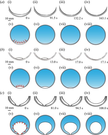
In our experiments, the time evolution of the hole is obtained from the bottom view by employing a high-speed camera. Moreover, we use a superhydrophobic glass plate (treated by Glaco Mirror Coat ‘Zero’, Soft 99, Co., see Appendix A) as the substrate, whereas we separately use three different kinds of wettability for the inner wall of the cylinder, i.e. superhydrophobic, hydrophobic and hydrophilic glasses. As illustrated in figure 3, typical experimental results of the wetting modes of holes at the wall are given, and three unexpected wetting modes are observed and can be generalized as follows.
Three wetting modes of holes at the wall. (a) Mode I; (b) mode II; (c) mode III. For each mode, panels (i–iv) are time-lapse images of the water layer with a hole, while panels (v–viii) are the schematics of the experimental observations corresponding to panels (i–iv), respectively. The red arrows denote the flow direction of the front of the liquid–vapour meniscus. The scale bar represents 10 mm.

In figure 3(a) wetting mode I is presented. In this case, both the glass plate and the inner wall of the container are superhydrophobic  $\theta = 158.2 \pm 3.0^{\circ }$. When adding water into the container, the hole is shrinking. Here, limited by the field of view of the camera, the experimental visualization (figure 3a i–iv) contains incomplete photographs of the container. Nevertheless, the main characteristic of the evolution of the hole can be captured. Figure 3(a v–viii) gives the sketches of mode I to demonstrate the complete view of the container, where the red arrows denote the flow direction of the front of the liquid–vapour meniscus. Confined by the container and the liquid–vapour interface, a crescent-shaped hole is formed. When more water is added to the liquid, the hole gradually gets smaller until it disappears (see supplementary movie 1 available at https://doi.org/10.1017/jfm.2023.753). In this case, the liquid film is always in a quasi-static state, which is different from the collapse of a hole located at the centre of a container reported previously (Diez et al. Reference Diez, Gratton and Gratton1992; Wilson & Duffy Reference Wilson and Duffy1996; Bankoff et al. Reference Bankoff, Johnson, Miksis, Schluter and Lopez2003; Dijksman et al. Reference Dijksman, Mukhopadhyay, Gaebler, Witelski and Behringer2015; Bostwick et al. Reference Bostwick, Dijksman and Shearer2017; Lv et al. Reference Lv, Eigenbrod and Hardt2018; Zheng et al. Reference Zheng, Fontelos, Shin, Dallaston, Tseluiko, Kalliadasis and Stone2018a,Reference Zheng, Fontelos, Shin and Stoneb).
In figure 3(b) wetting mode II is presented. In this case, the glass plate is superhydrophobic ( $\theta = 158.2 \pm 3.0 ^{\circ }$), while a cylindrical glass with a hydrophobic inner wall (
 $\theta = 116.0 \pm 1.9 ^{\circ }$) is employed. In contrast to mode I, an eye-shaped hole is formed (see supplementary movie 2). Here, the flow rate of the nozzle is
 $Q = 0.1\,\mathrm {ml}\,\mathrm {min}^{-1}$ when adding water into the water film, which guarantees a very smooth shrinking of the hole. In the beginning, the time evolution of the appearance of the hole is hardly observed by the naked eye, i.e. from 0 to 13.0 s, therefore, the hole is in a quasi-static state in this regime. However, as time progresses, the situation will change when the hole size approaches a critical value. Since the geometrical shape of the hole is not regular, we use an area
 $A(t)$ to describe the geometry of the hole, where
 $A(t)$ is the projected area of the hole. As the hole area
 $A(t)$ decreases to a critical value
 $A_c$, the hole is no longer able to hold its stability, but collapses, i.e. the area
 $A(t)$ suddenly reduces to zero (from 17.0 to 17.1 s). The stability and collapse of the hole in mode II are very similar to the observations of Lv et al. (Reference Lv, Eigenbrod and Hardt2018).
In figure 3(c) wetting mode III is presented. In this case, the glass plate is superhydrophobic ( $\theta = 158.2 \pm 3.0 ^{\circ }$), while a cylindrical glass with a hydrophilic inner wall (
 $\theta = 29.7 \pm 5.8 ^{\circ }$) is employed. The water film wets the inner wall of the cylinder as much as possible but decreases the contact area with the substrate. Different from wetting modes I and II, the front of the water film spreads more quickly along the inner wall of the cylinder than on the glass plate (see supplementary movie 3), and a funnel-shaped hole appears (from 0 to 94.5 s). Eventually, the left and right fronts of the water film merge at the wall, and a transition from a hole at the wall to an inner hole happens, and the hole is pushed a little further from the inner wall of the cylinder. Meanwhile, we observe that the hole reshapes itself to a circle shape soon after the transition. This behaviour has not been observed previously (Lv et al. Reference Lv, Eigenbrod and Hardt2018; Zheng et al. Reference Zheng, Fontelos, Shin, Dallaston, Tseluiko, Kalliadasis and Stone2018a,Reference Zheng, Fontelos, Shin and Stoneb).
To the best of our knowledge, this is the first report of the different wetting behaviours of the hole in the liquid layer. Although liquid layers were widely studied in the past, most of them focused on the hole occurring in the centre of the container (Wilson & Duffy Reference Wilson and Duffy1996; Bankoff et al. Reference Bankoff, Johnson, Miksis, Schluter and Lopez2003; Dijksman et al. Reference Dijksman, Mukhopadhyay, Gaebler, Witelski and Behringer2015; Bostwick et al. Reference Bostwick, Dijksman and Shearer2017; Lv et al. Reference Lv, Eigenbrod and Hardt2018; Zheng et al. Reference Zheng, Fontelos, Shin, Dallaston, Tseluiko, Kalliadasis and Stone2018a,Reference Zheng, Fontelos, Shin and Stoneb), or the dependence of the collapse behaviours on the viscosity of the liquid (Redon et al. Reference Redon, Brochard-Wyart and Rondelez1991; Diez et al. Reference Diez, Gratton and Gratton1992; Zheng et al. Reference Zheng, Fontelos, Shin, Dallaston, Tseluiko, Kalliadasis and Stone2018a,Reference Zheng, Fontelos, Shin and Stoneb; Lu & Corvalan Reference Lu and Corvalan2019; Lu et al. Reference Lu, Ferri, Ubal, Campanella and Corvalan2019) and the wettabilities of the container (Redon et al. Reference Redon, Brochard-Wyart and Rondelez1991; Lv et al. Reference Lv, Eigenbrod and Hardt2018). Here, our observations are distinguished from the previous experimental results.
2.2.2. Experimental analysis
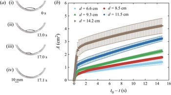
In order to quantify the dynamics of the hole, we plot the relationship between the instantaneous value of  $A$ and time
 $(t_0 - t)$, denoting
 $t_0$ the moment when
 $A = 0$. As shown in figures 4 and 5, we plot the results for modes I and II, respectively.
Wetting mode I. (a) Selected frames from the top view. Glaco-treated glasses are used as the planar substrate and the cylindrical wall of the container. The scale bar represents 10 mm. (b) Time evolution of the hole area in a liquid layer for wetting mode I. Glaco-treated glasses are used as the planar substrate and the cylindrical wall of the container. The plot shows the instantaneous area  $A$ of the hole as a function of time
 $(t_0 - t)$, where
 $t_0$ is defined as the moment when
 $A = 0$. All the data points are average values of five experiments with error bars representing the standard deviation.

Wetting mode II. (a) Selected frames from the experiment of wetting mode II. A planar Glaco-treated glass is used as the substrate, while a cylindrical hydrophobic glass is used as the wall of the container. The scale bar represents 10 mm. (b) Evolution of the instantaneous area  $A$ with time
 $(t_0 - t)$ for wetting mode II.
 $t_0$ is defined as the moment when
 $A = 0$. A plastic Petri dish is used as the container. All the data points are average values of five experiments with error bars representing the standard deviation. Five containers with a diameter
 $d$ ranging from 6.6 to 14.2 cm have been employed.

As shown in figure 4, we first demonstrate the behaviour of wetting mode I. Here, Glaco-treated glasses are used as the planar substrate and the cylindrical wall of the container, which provide an advancing contact angle  $\theta _a = 163.3 \pm 1.0^{\circ }$ and a receding contact angle
 $\theta _r = 151.8 \pm 2.4^{\circ }$. Selected frames are displayed in figure 4(a), showing the time evolution of the hole shape in bottom view, indicating that the solid–liquid–vapour three-phase contact lines gently move forwards. Based on the experimental data shown in figure 4(b), it is found that the hole shrinks uniformly when water is added. Owing to the contact line pinning, the curve is not as smooth as a straight line and there is jerky glide motion observed in supplementary movie 1.
As shown in figure 5(a), we demonstrate the behaviour of wetting mode II. Here, a cylindrical hydrophobic glass is used as the wall of the container, which provides an advancing contact angle  $\theta _a = 119.3 \pm 1.3^{\circ }$ and a receding contact angle
 $\theta _r = 105.8 \pm 2.2^{\circ }$. Moreover, a planar Glaco-treated glass is used as the substrate, which provides an advancing contact angle
 $\theta _a = 163.3 \pm 1.0^{\circ }$ and a receding contact angle
 $\theta _r = 151.8 \pm 2.4^{\circ }$. In figure 5(b),
 $A$ is plotted as a function of time
 $(t_0 - t)$ for a range of box sizes, where the data points were obtained by averaging five experiments with corresponding error bars. Here, the plastic Petri dish is used as the container, which provides an advancing contact angle
 $\theta _a = 102.7 \pm 0.7^{\circ }$ and a receding contact angle
 $\theta _r = 80.5 \pm 1.6^{\circ }$. Five different containers with diameters
 $d$ ranging from 6.6 to 14.2 cm have been employed. The curves for wetting mode II shown in figure 5(b) contain two regimes. In the first regime, the area of the hole decreases smoothly with time corresponding to the photographs from 0 to 13.0 s (see supplementary movie 2). In this process, the shrinking of the hole is due to the feeding of water. Since water is added at very small flow rate, the shrinking of the hole is not obvious. Here, it is stressed that, when the feed is stopped, the shrinking of the hole stops correspondingly and the liquid is in a static state. In this regard, the hole is considered to be stable. However, when the hole shrinks to a critical size, a subsequent volume increase will trigger the collapse of the hole. The second regime happens at this time. As shown in figure 5(b), the area of the hole steeply decreases with time corresponding to the photographs from 17.0 to 17.1 s. During the second stage, the hole cannot remain static even we stop adding water. In this process, the hole collapse is highly dynamic in contrast to the first regime. Although containers with different sizes are used, the curves in figure 5(b) have the same trend.
Before we carry out systematic theoretical analyses (see § 4) for these three wetting modes, an intuitive understanding could be obtained. For the meniscus of the hole, there are two principal curvatures, i.e. the azimuthal curvature (see the top view in figure 1a) and the meridional curvature (see the side view in figure 1b). Therefore, for the wetting mode I, as shown in figure 3(a), both the two curvatures are positive, which create a pressure jump together to maintain the opening of the hole. As a result, the hole is able to be stable until it closes. However, for the wetting mode II, as shown in figure 3(b), the azimuthal curvature becomes negative to push the liquid to the hole. As additional liquid is supplied, the increase of the azimuthal curvature is pronounced while the variations of the meridional curvature and the hydrostatic pressure are relatively small. Therefore, the collapse of the liquid layer is caused by the variation of the azimuthal curvature. Lastly, for wetting mode III, as shown in figure 3(c), when adding enough liquid, the front liquid menisci must merge together. To further decrease the energy of the system, the hole will trend to become circular and meanwhile it seems the hole is pushed along the central direction of the container.
3. Numerical study
Even though the above experiment results reveal three different wetting modes of holes at the wall in the liquid layers, the experimental study is limited by the wetting properties of the materials we used for the wall and the substrate of the container, thus, only a limited number of experimental parameters are available. In order to expand the parameters, we will employ numerical method to carry out more investigations in this section. Here, two numerical methods, SE and LBM, are employed to simulate the behaviour of a bounded liquid layer with a hole.
3.1. Surface evolver simulation
We first employ a public domain software package SE (Brakke Reference Brakke1992) to simulate holes at the wall in liquid layers. The basic concept of SE is to minimize the energy and find the equilibrium shape of a liquid volume surface with given parameters such as the surface tension and stiffness, subjected to external forces (e.g. gravity, centrifugal force, magnetic force) and constraints (e.g. volume conservation, contact angle, pinning of the contact line). The SE has been widely applied to studying various interfacial phenomena (such as morphologies of droplets and particles (Cho et al. Reference Cho, Yi, Lim, Kim, Manoharan, Pine and Yang2005; Crawford, Lim & Gradecak Reference Crawford, Lim and Gradecak2013; Lv et al. Reference Lv, Chen, Chuang, Tseng, Yin, Grey and Zheng2014; Dević et al. Reference Dević, Encarnación, José and Lohse2019; Lv & Hardt Reference Lv and Hardt2021; Chu et al. Reference Chu, Zhao, Hao and Lv2023), foams (Kabla & Debregeas Reference Kabla and Debregeas2007) as well as the equilibrium configuration of biomembranes (Michalet Reference Michalet2007; Sakashita et al. Reference Sakashita, Urakami, Ziherl and Imai2012), with excellent agreement with experimental results. However, for our problem, SE could only simulate static or quasi-static problems and could not take dynamic behaviour into consideration. As we analysed in § 2.1, the influence of the flow rate on the evolution of the liquid layer is negligible and the liquid layer is in the quasi-static state before collapse. Therefore, we propose the convenient simplification of reducing the problem to a succession of quasi-static liquid profiles.
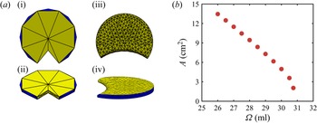
As shown in figure 6(a), we give the results of the configuration of the liquid film simulated by SE. For a given volume  $\varOmega$ of the liquid layer, two configurations from different views on the left and the right panels demonstrate the initial and the final configurations of the liquid layer, respectively (for more details of the SE simulations, see S1 in the supplementary information). Moreover, further information such as the areas of the liquid–vapour and the solid–liquid interfaces, as well as the potential of the system, can be extracted based on the final configuration. By the help of SE, a series of stable liquid layers with different volumes
 $\varOmega$ can be obtained.
Schematic sketch of SE simulation. (a) The evolution of a liquid layer simulated by SE. The yellow and blue colours represent the liquid–vapour and solid–liquid interfaces, respectively. The two configurations from different views in panels (a i,a ii) and (a iii,a iv) demonstrate the initial and the final configurations of the liquid layer, respectively. (b) Results obtained from SE simulation showing dependency of  $A$ on
 $\varOmega$, with
 $A$ and
 $\varOmega$ being the area of the hole and the volume of water, respectively. The contact angles of the substrate and the wall are
 $\theta _s = 160^{\circ }$ and
 $\theta _w = 90^{\circ }$, respectively. The diameter of the container is
 $d = 9 \, \mathrm {cm}$.

As presented in figure 6(b), the relationship between the hole area  $A$ and the liquid volume
 $\varOmega$ is given. Here, the container diameter is fixed at
 $d = 9 \, \mathrm {cm}$, and the contact angles of the substrate and the wall of the container are set to
 $\theta _s = 160^{\circ }$ and
 $\theta _w = 90^{\circ }$, respectively. Each point in figure 6(b) represents a static configuration of the system. It is shown that the area of the hole
 $A$ first decreases linearly with the volume
 $\varOmega$ of the liquid. However, when
 $\varOmega$ exceeds a critical value
 $\varOmega _c$ (which corresponds to a critical area
 $A_c$), we can never obtain a static liquid layer with a hole. Actually, we cannot precisely determine the threshold of the collapse of the hole. Therefore, we artificially define the threshold of the collapse of the hole in which a further 1 % increase in liquid volume will trigger the hole closure. Thus, the last point
 $(\varOmega _c, A_c)$ in figure 6(b) is considered to be the threshold accounting for the collapse of the hole. Close to the critical point, the linear relation between
 $A$ and
 $\varOmega$ is not maintained and the slope of the simulation data suddenly increases.
Moreover, the effect of the size of the container is investigated by considering five diameters from  $d = 7$ to 15 cm. For each diameter of the container with certain wettability, a series of simulations with different liquid volumes are conducted. Specifically, we first give a sufficiently small volume
 $\varOmega$ of liquid (in other words, a liquid layer with a larger hole) in our simulations and then obtain the equilibrium wetting state of the system. After that, we continuously increase the liquid volume to find the corresponding equilibrium wetting state, until we find the critical volume
 $\varOmega _c$. Figure 7(a) shows the top views of outcomes of
 $d = 9$ cm with different liquid volumes, from which we can see that an eye-shaped hole appears in each case. Similarly, equilibrium wetting states of liquid layers in containers with other diameters can be obtained. Figure 7(b) shows the outcomes of SE simulations with different container diameters, and when given proper liquid volumes, eye-shaped holes with similar shapes appear, which indicates that the wetting state of the liquid is not affected by the size of the container.
The snapshots of liquid layer. The contact angles of the substrate and the wall are  $\theta _s = 160^{\circ }$ and
 $\theta _w = 90^{\circ }$, respectively. (a) Configuration of the liquid with the volume. The diameter of the container is fixed at
 $d = 9\,\mathrm {cm}$. (b) The diameter of the container
 $d$ ranges from 7 to 15 cm. The configurations correspond to the thresholds of the collapse of the hole.

Furthermore, the simulation data for containers with diameters  $d$ are shown in figure 8, in which five diameters
 $d$ ranging from 7 to 15 cm are presented with different colours and shapes. Here, the wettability of the container is fixed, i.e. the contact angles of the substrate and the wall of the container are
 $\theta _s = 160^{\circ }$ and
 $\theta _w = 90^{\circ }$, respectively. We can see that all the data have similar trends no matter the value of the diameter of the container. However, each set of the data has a group of thresholds
 $(\varOmega _c, A_c)$, and these thresholds depend on the container diameter. The threshold values will be analysed theoretically in the following sections.
Dependency of the hole area  $A$ on liquid volume
 $\varOmega$ for various diameters of the container obtained by SE simulations. In this case, a circular container with
 $\theta _s = 160^{\circ }$ and
 $\theta _w = 90^{\circ }$ has been considered, denoting with
 $\theta _s$ and
 $\theta _w$ the contact angles of the substrate and the wall of the container, respectively. Different container diameters
 $d$ = 7 cm, 9 cm, 11 cm, 13 cm and 15 cm are employed.

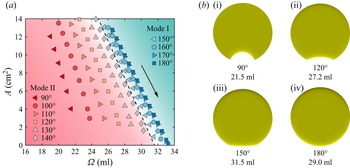
Next, the influence of the wettability on the wetting property of the liquid layer is systematically investigated. For the sake of simplicity, let the contact angles of the substrate and the wall of the container have the same value, i.e.  $\theta _s = \theta _w$. As shown in figure 9, we consider contact angles ranging from
 $90^{\circ }$ to
 $180^{\circ }$. Here, the diameter of the container is fixed at
 $d = 9$ cm. There is a remarkable difference of the wetting behaviour of the liquid layer between different contact angles. Each set of the data has a group of thresholds
 $(\varOmega _c, A_c)$, which depends on the contact angle. Moreover, the phase diagram of parameter space can be divided into two parts, which correspond to wetting modes I and II, and the boundary between mode I and mode II is
 $\theta _s = \theta _w = 145^{\circ }$ (see the dashed line). Here, we artificially define the criterion to distinguish mode I and mode II based on the following: when
 $A_c$ is smaller than 1 % of the projected area of the container, it is mode I; otherwise, it is mode II. In our SE simulations, when
 $\theta _s=\theta _w>145^{\circ }$, we found
 $A_c$ is very close to zero and it is not visually discernible. However, when
 $\theta _s = \theta _w < 145^{\circ }$, when the hole area is smaller than an obvious value of
 $A_c$ (with a maximum value
 $\varOmega _c$), we can never find a stable liquid layer, i.e. a slight 1 % increase in liquid volume will trigger the closure of the hole. The results shown in figure 9 demonstrate that the threshold value accounting for the collapse of the hole is closely related to the wetting property of the container.
(a) Dependency of  $A$ on
 $\varOmega$ for various wettabilities of the container obtained from SE simulations. Here, a circular container with
 $d$ = 9 cm has been considered, with contact angles of
 $\theta _s=\theta _w=90^{\circ }$,
 $100^{\circ }$,
 $110^{\circ }$,
 $120^{\circ }$,
 $130^{\circ }$,
 $140^{\circ }$,
 $150^{\circ }$,
 $160^{\circ }$,
 $170^{\circ }$ and
 $180^{\circ }$. The arrow indicates the direction in which the volume
 $\varOmega$ is increasing. (b) Snapshots of the liquid profile from the top view when the threshold of collapse is reached. Examples with different contact angles
 $\theta _s=\theta _w=90^{\circ }$,
 $120^{\circ }$,
 $150^{\circ }$ and
 $180^{\circ }$ are demonstrated, which are obtained from SE simulations.

Despite the influence of the wettability on the instability of the hole as discussed in the above, the wettabilities of the substrate and the wall of the container have not been considered separately. As shown in figure 10, we investigate the influence of the wettability on the instability of the hole solely resulting from the substrate or the wall of the container. The snapshots in figure 10 demonstrate the thresholds of instability of the liquid layer in containers. Figure 10(a) shows a series of results where the contact angle of the container substrate is fixed at  $\theta _s = 160^{\circ }$ while the contact angle of the container wall is varied as
 $\theta _w = 60^{\circ }$,
 $90^{\circ }$ and
 $160^{\circ }$. We can see that there exists an obvious eye-shaped hole for a small value of
 $\theta _w$ when the threshold of instability is reached. However, with an increase of
 $\theta _w$, the size of the crescent-shaped hole becomes smaller and it is even indiscernible when
 $\theta _w$ is large enough (i.e.
 $\theta _w = 160^{\circ }$). Moreover, figure 10(b) shows the cases where the contact angle of the container wall is fixed at
 $\theta _w = 90^{\circ }$ while the contact angle of the container substrate is varied as
 $\theta _s = 60^{\circ }$,
 $90^{\circ }$ and
 $160^{\circ }$. We can see in this case that, even though the value of
 $\theta _s$ is varied over a wide range, an obvious eye-shaped hole always exists when the threshold of the instability is reached. In this regard, the instability of the liquid layer is mainly influenced by
 $\theta _w$ rather than
 $\theta _s$, and this conclusion is consistent with our experimental observations in § 2.2 where the substrate is fixed but the wall of the container is changed.
Snapshots showing the thresholds of instability of the liquid layer in containers with different contact angles. Here, the diameter of the container is  $d = 9$ cm. (a) The contact angle of the substrate is fixed at
 $\theta _s = 160^{\circ }$ and the contact angle of the wall is varied as
 $\theta _w = 60^{\circ }$,
 $90^{\circ }$ and
 $160^{\circ }$. (b) The contact angle of the wall is fixed at
 $\theta _w = 90^{\circ }$ and the contact angle of the substrate is varied as
 $\theta _s = 60^{\circ }$,
 $90^{\circ }$ and
 $160^{\circ }$.

3.2. Lattice Boltzmann method
Although SE gives a distinct picture of wetting mode I and wetting mode II, wetting mode III is still not considered. As shown in our experimental observations in § 2.2, wetting mode III happens in a hydrophilic condition of the container and involves a dynamics which is beyond the capability of SE (see the supplementary information). Therefore, we employ another numerical method, i.e. LBM, to simulate wetting mode III. Details of how we realize simulations via LBM is given in the supplementary information. Here, we only demonstrate the main results.
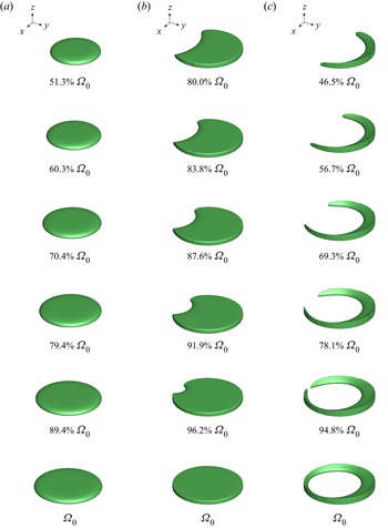
As shown in figure 11, we perform simulations for two-phase flows under gravity and surface tension. The simulations include the three wetting modes we have observed in experiments, which are realized by assigning certain values of the contact angle to the substrate and the wall of the container. Specifically, we assign ( $\theta _s = 120^{\circ }$,
 $\theta _w = 180^{\circ }$), (
 $\theta _s = 120^{\circ }$,
 $\theta _w = 90^{\circ }$) and (
 $\theta _s = 120^{\circ }$,
 $\theta _w = 35^{\circ }$) in figures 11(a), 11(b) and 11(c), respectively. The snapshots demonstrate the time evolution of the liquid layers with its volume. As shown in figure 11(a), when
 $\theta _w = 180^{\circ }$, the hole is shrinking very smoothly when feeding more liquid into the container, until the liquid layer entirely fills the container. However, as shown in figure 11(b), when
 $\theta _w = 90^{\circ }$, the hole is shrinking smoothly in the first stage, and then reaches a critical state. After that, the hole suddenly collapses with a further increase of the liquid volume. Furthermore, as shown in figure 11(c), when
 $\theta _w = 35^{\circ }$, with a continuous increase of the liquid volume, the liquid first spreads along the junction of the substrate and the wall. When enough liquid is added, the liquid forms a ring-like structure including a hole inside, but meanwhile the hole is suddenly pushed into the central direction of the container. The simulation results (see supplementary movies 4–6) very well reproduce the experimental observations. Here, it is stressed that, in both the numerical simulations and experiments, despite the collapse that causes the hole to be pushed towards the centre of the container, the hole consistently maintains a certain distance from the wall and is not located right in the centre of the container.
Snapshots showing time evolution of liquid layer with its volume which are simulated by employing LBM. The final volume of the liquid layer for each mode is defined as  $\varOmega _0$. Here, the contact angle of the substrate of the container is fixed at
 $\theta _s = 120^{\circ }$, while three different contact angles of the wall of the container are simulated. The diameter of the container is
 $d \approx 60$ mm. (a) Wetting mode I (
 $\theta _s = 120^{\circ }$,
 $\theta _w = 180^{\circ }$); (b) wetting mode II (
 $\theta _s = 120^{\circ }$,
 $\theta _w = 90^{\circ }$); (c) wetting mode III (
 $\theta _s = 120^{\circ }$,
 $\theta _w = 35^{\circ }$).

By employing LBM simulations, we systematically investigate the influence of wettability on the wetting modes. The dots represent the simulation results as shown in figure 12. Specifically, we fix the contact angle of the container substrate  $\theta _s$ ranging from
 $15^{\circ }$ to
 $175^{\circ }$, and we choose a high value of the contact angle of the container wall
 $\theta _w = 175^{\circ }$, then we obtain the results of wetting mode I. After that, we gradually decrease the contact angle
 $\theta _w$ for each
 $\theta _s$ until wetting mode II appears. By employing this method, we not only find the parameter regime of wetting mode I, we also find the boundary (the upper dashed curve) between wetting modes I and II, which is determined by averaging the neighbouring contact angles and the dashed curve is extended by employing a fitting. After further decreasing the value of
 $\theta _w$, we obtain the parameter regime of wetting mode II, as well as the boundary between wetting modes II and III. After we obtain enough data, we are able to plot a phase diagram in terms of the contact angles
 $\theta _w$ and
 $\theta _s$ which includes the three wetting modes. Based on the results shown in figure 12, we can see the wetting mode is mainly determined by the contact angle of the wall of the container, i.e.
 $\theta _w$. Generally, when
 $\theta _s$ takes a relatively large value (i.e.
 $\theta _s > 90^{\circ }$), the two boundaries occur at
 $\theta _w \approx 45^{\circ }$ and
 $\theta _w \approx 145^{\circ }$. However, when
 $\theta _s$ takes a relatively small value (i.e.
 $\theta _s < 90^{\circ }$), the situation is more complex, the regime of wetting mode II declines but the regimes of wetting modes I and II increase.
Phase diagram illustrated in terms of  $\theta _s$ and
 $\theta _w$ showing the wetting modes obtained by LBM simulations. The triangles, squares and circles denote wetting modes I, II and III, respectively. The two dashed curves represent the boundaries between the neighbouring wetting modes. The diameter of the container is
 $d \approx 60$ mm. The dashed line in the region for small
 $\theta _s$ (i.e.
 $\theta _s < 15^{\circ }$) is an educated guess.

4. Theoretical model
In order to understand the underlying mechanisms, we carry out theoretical analyses in the following. In our theoretical model, relevant factors such as the contact angles of the substrate and the wall of the container, gravity as well as the sizes of the hole at the wall and the container, will be considered. As mentioned in the above, since the influence of the flow rate is negligible, we treat the wetting state of the liquid layer with a hole as quasi-static. Therefore, the problem is simplified to a static problem.
In this regard, the profile of the liquid–vapour interface is controlled by the Young–Laplace equation (de Gennes et al. Reference de Gennes, Brochard-Wyart and Quéré2003)
 \begin{equation} \Delta p = \gamma\left ( \frac{1}{R_1} + \frac{1}{R_2} \right ). \end{equation}
When we choose any point on the liquid–vapour interface,  $\Delta p$ is the pressure difference between the two sides of the liquid–vapour interface,
 $\gamma$ is surface tension and
 $R_1$ and
 $R_2$ are the two principal radii of curvature of the liquid–vapour interface. For example, when we choose a point at the equator of the hole,
 $1/R_1$ and
 $1/R_2$ denote the azimuthal curvature and the meridional curvature, respectively.
However, exact (non-trivial) solutions of the Young–Laplace equation including gravity are limited to two specific cases: (i) a fluid in a semi-infinite domain bounded by a vertical plane wall; (ii) a fluid between two vertical parallel walls (Landau & Lifshitz Reference Landau and Lifshitz1987; Norbury, Sander & Scott Reference Norbury, Sander and Scott2005; Lv & Shi Reference Lv and Shi2018). For an axisymmetric coordinate container with a hole in the centre, asymptotic models for small contact angles were obtained in the past (López et al. Reference López, Miksis and Bankoff2001; Lv et al. Reference Lv, Eigenbrod and Hardt2018). Since our problem is a non-axisymmetric system, the asymptotic methods developed in the past (López et al. Reference López, Miksis and Bankoff2001; Lv et al. Reference Lv, Eigenbrod and Hardt2018) cannot be directly applied to this study. In § 4.1, we will establish a simple model where the liquid layer is considered to be flat. When we minimize the energy of the system, we can obtain the static profile of the liquid layer. Moreover, the outcomes of the model will be presented in § 4.2.
4.1. Theoretical model
Here, in our theoretical analysis, we consider the case of wetting modes I and II. To obtain the potential of the system from a theoretical point of view, we assume on the one hand that the liquid–vapour interface is perpendicular to both the substrate and the wall, and on the other hand that the edge of the hole is circular, as sketched in figure 13. The former assumption is based on the large ratio between the container diameter and the thickness of the liquid layer. In the smallest container ( $d = 6.6$ cm), the thickness of the liquid layer is approximately
 $2l_c \approx 5.46$ mm. Therefore, the ratio between the thickness and the width of the liquid layer is approximately 0.08 (
 $\ll 1$), which suggests that the variation of the meniscus thickness around the edge of the hole may have little influence on the energy of the system (see the supplementary information). The latter assumption about a circular shape of the hole is based on the observation in the experiments and simulations.
Simplified liquid layer profile shown from oblique view (a) and top view (b). Relevant geometric parameters are defined.

When additional liquid is fed into the liquid layer, at a specific time, the liquid has a specific volume  $\varOmega$. The free energy of the system can be written as
 $E = E_s + E_g = A_{lv} \gamma + A_{sl} ( \gamma _{sl} - \gamma _{sv} ) + \rho \varOmega g h/2$. Here,
 $\rho$ and
 $g$ represent the mass density of the liquid and the gravitational acceleration respectively,
 $E_s = A_{lv} \gamma + A_{sl} ( \gamma _{sl} - \gamma _{sv} )$ and
 $E_g = \rho \varOmega g h/2$ represent the surface energy and the gravity potential, respectively, with
 $h$ being the thickness of the liquid layer. Further,
 $A_{lv}$ and
 $A_{sl}$ represent the liquid–vapour area and the solid–liquid area respectively, and
 $\gamma$,
 $\gamma _{sl}$ and
 $\gamma _{sv}$ represent the liquid–vapour, solid–liquid and solid–vapour interfacial tensions, respectively. The basic idea is that, for given parameters such as
 $d$,
 $\rho$,
 $g$,
 $\gamma$,
 $\gamma _{sl}$ and
 $\gamma _{sv}$, we will find the solution when the total energy
 $E$ reaches a minimum
 $E_{min}$ under the constraint of the certain volume
 $\varOmega$, as well as the geometric relationships as shown in figure 13(b). When we obtain a wetting state which satisfies
 $E = E_{min}$, we find the equilibrium wetting state of the liquid layer.
The geometry parameters are presented in figure 13(b), in which  $\alpha$ and
 $\beta$ are the half-angles of the liquid and the hole satisfying the relationship
 $\theta _w + \alpha + \beta = {\rm \pi}$. In addition,
 $A_1$ represents the area of the upper liquid–vapour interface, which is equal to the corresponding liquid–substrate interface, and
 $A_2$ and
 $A_3$ represent the areas of the side liquid–vapour interface at the boundary of the hole and the area of the side liquid–wall interface, respectively. These areas can be written as
 $A_1 = r_1^2 ( {\rm \pi}-\alpha + \sin \alpha \cos \alpha ) - r_2^2 ( \beta - \sin \beta \cos \beta )$,
 $A_2 = 2 r_2 \beta h$ and
 $A_3 = 2r_1 ( {\rm \pi}- \alpha ) h$, where
 $r_1$ and
 $r_2$ are the radii of the liquid and the hole satisfying
 $r_1 \sin \alpha = r_2 \sin \beta$.
Moreover, the surface energy  $E_s$ consists of the liquid–vapour surface energy, the solid–liquid and the solid–vapour surface energy, which can be written as
 \begin{align} E_s & = A_1 \gamma + A_1
( \gamma_{sl}^s - \gamma_{sv}^s ) + A_2 \gamma
+A_3 ( \gamma_{sl}^w - \gamma_{sv}^w ) \nonumber\\ & = A_1 \gamma \left ( 1 - \cos \theta_s \right
) + A_2 \gamma - A_3 \gamma \cos \theta_w ,
\end{align}
where the second equation uses the Young equation as  $\cos \theta _s = ( \gamma _{sv}^s - \gamma _{sl}^s ) / \gamma$ and
 $\cos \theta _w = ( \gamma _{sv}^w - \gamma _{sl}^w ) / \gamma$. The superscripts
 $s$ and
 $w$ represent the substrate and the wall, respectively.
For convenience, by employing the radius of the liquid layer  $r_1$ (in other words, the radius of the container), we define dimensionless forms of the relevant geometric and physical quantities
 \begin{equation} \left. \begin{aligned} & \displaystyle \tilde{h} \equiv \frac{h}{r_1},\quad \tilde{A}_1 \equiv \frac{A_1}{r_1^2},\quad \tilde{A}_2 \equiv \frac{A_2}{r_1^2},\quad\tilde{A}_3 \equiv \frac{A_3}{r_1^2},\\ & \displaystyle \tilde{\varOmega} \equiv \frac{\varOmega}{r_1^3} ,\quad \tilde{E}_s \equiv \frac{E_s}{r_1^2 \gamma},\quad \tilde{E}_g \equiv \frac{E_g}{r_1^2 \gamma}, \end{aligned} \right\} \end{equation}
and we rewrite  $\tilde {A}_1$,
 $\tilde {A}_2$,
 $\tilde {A}_3$,
 $\tilde {E}_s$ and
 $\tilde {E}_g$ into
 \begin{gather} \tilde{A}_1 = \left( {\rm \pi}-\alpha + \sin \alpha \cos \alpha \right) - \frac{\sin^2\alpha}{\sin^2\beta} \left( \beta - \sin \beta \cos \beta \right), \end{gather}
 \begin{gather} \tilde{A}_2 = 2 \frac{\sin\alpha}{\sin\beta} \beta \tilde{h}, \end{gather}
 \begin{gather} \tilde{A}_3 = 2 \left ( {\rm \pi}- \alpha \right ) \tilde{h}, \end{gather}
 \begin{gather} \tilde{E}_s = \tilde{A}_1\left ( 1 - \cos \theta_s \right ) + \tilde{A}_2 - \tilde{A}_3 \cos \theta_w, \end{gather}
 \begin{gather} \tilde{E}_g = \frac{1}{2} \tilde{\varOmega} \tilde{h} \left ( \frac{r_1}{l_c} \right )^2. \end{gather}
In order to obtain the equilibrium profile of the liquid, we calculate the derivative of the energy in term as  $\alpha$, and let
 \begin{equation}
\frac{\partial \tilde{E}}{\partial \alpha}=\frac{\partial(\tilde{E}_s+\tilde{E}_g)}{\partial
\alpha}=0. \end{equation}
In addition, considering the constraint
 \begin{equation} \tilde{\varOmega}=\tilde{A}_1 \tilde{h}=\mathrm{constant}, \end{equation}
we have  $\partial \varOmega / \partial \alpha = 0$, thus, the following relation can be obtained:
 \begin{equation} \frac{\partial \tilde{h}}{\partial \alpha}={-}\frac{\tilde{h}}{\tilde{A}_1} \frac{\partial \tilde{A}_1}{\partial \alpha}. \end{equation}
Substituting equations (4.4)–(4.8) and (4.11) into (4.9), we obtain the dimensionless value of the liquid layer thickness
 \begin{align} \tilde{h} & = \frac{\partial \tilde{A}_1}{\partial \alpha}\left(1-\cos \theta_s\right) \left\{ \left[2 \beta \frac{\sin \alpha}{\sin \beta} - 2\left({\rm \pi}-\alpha\right) \cos \theta_w+ \frac{1}{2} \tilde{\varOmega} \left(\frac{r_1}{l_c}\right)^2\right] \frac{1}{\tilde{A}_1} \frac{\partial \tilde{A}_1}{\partial \alpha} \right. \nonumber\\ &\quad \left. +\,2 \frac{\sin \alpha}{\sin \beta} - \frac{2 \beta}{\sin ^2 \beta}\left(\sin \alpha \cos \beta + \cos \alpha \sin \beta\right) - 2 \cos \theta_w \right\}^{{-}1}, \end{align}
where
 \begin{align} \frac{\partial \tilde{A}_1}{\partial \alpha} & = 2\frac{\sin ^2 \alpha}{\sin ^2 \beta} - 2 \beta\left(\frac{\sin \alpha \cos \alpha}{\sin ^2 \beta} + \frac{\sin ^2 \alpha \cos \beta}{\sin ^3 \beta}\right) + 2\frac{\sin \alpha \cos \alpha \cos \beta}{\sin \beta} \nonumber\\ &\quad +\cos ^2 \alpha-\sin ^2 \alpha-1. \end{align}
The solution of the problem is solved based on the following line of thought. Putting (4.4) and (4.12) into (4.10), and considering  $\theta _w + \alpha + \beta = {\rm \pi}$, we can see there is only one unknown parameter
 $\alpha$. By employing a shooting method carried out by Matlab,
 $\alpha$ can be obtained. Based on that,
 $\beta$ can be obtained from
 $\theta _w + \alpha + \beta = {\rm \pi}$, moreover, the other unknown interested parameters such as
 $h$,
 $E_s$ and
 $E_g$ can be obtained based on the (4.12), (4.7) and (4.8).
It is stressed that, when  $\theta _w = 180^{\circ }$ (even though it is difficult to achieve in practical cases, it is meaningful from a theoretical point of view), we cannot find the solution of the problem based on (4.12) because some singularities exist in the algebraic equations. Therefore, the condition for
 $\theta _w = 180^{\circ }$ should be considered specifically, and the details are shown in Appendix B. For this case, we obtain the following relationship:
 \begin{equation} \tilde{h}=\frac{{\rm \pi} \tilde{r}^2\left(1-\cos \theta_s\right)}{\displaystyle {\rm \pi}\tilde{r}+\frac{1}{2} \tilde{\varOmega}\left(\frac{r_1}{l_c}\right)^2}. \end{equation}
Here, we emphasize that the theory developed in the above is exclusively applicable to the quasi-static evolution of the hole in wetting modes I and II.
4.2. Results from the theoretical model
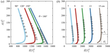
Since we have derived a simple model to obtain the equilibrium wetting state of the liquid layers, as illustrated in figure 14, two cases are studied (the dense data): (i) liquid layers in a circular container with diameter  $d =$ 9 cm, but with contact angles
 $\theta _s = \theta _w$ ranging from
 $90^{\circ }$ to
 $180^{\circ }$; (ii) liquid layers in a container with unchangeable wettability (
 $\theta _s = 160^{\circ }$ and
 $\theta _w = 90^{\circ }$) but with diameters ranging from
 $d =$ 7 cm to 15 cm. The black hollow circles are numerical solutions obtained by SE with corresponding values of the wettability and the size of the container. The good agreement between the theoretical and SE results verifies the rationality of our assumptions in the simple theoretical model. In figure 14(a), two shapes of curves are obtained: (i) when
 $\theta _s = \theta _w = 90^{\circ }$,
 $120^{\circ }$ and
 $150^{\circ }$, the dimensionless area
 $A/l_c^2$ does not monotonically change with the dimensionless volume
 $\varOmega /l_c^3$; (ii) when
 $\theta _s = \theta _w = 180^{\circ }$, there is a monotonic relationship between
 $A/l_c^2$ and
 $\varOmega /l_c^3$. For the former case, when the hole area is relatively large, the liquid volume
 $\varOmega$ increases with decreasing
 $A$. However, there is a maximum volume
 $\varOmega _c$ which corresponds to a critical value of
 $A_c$. According to the minimum-volume theorem proposed by Langbein (Reference Langbein2002), the point (
 $\varOmega _c$,
 $A_c$) corresponds to a point of instability. The smaller
 $A$ is energetically unstable, which cannot be obtained in experiment or simulation. In other words, if
 $A < A_c$, solutions of (4.12) exist mathematically, but they are physically unstable (Moriarty & Schwartz Reference Moriarty and Schwartz1993). In our experiment, the volume of the liquid monotonically increases until it reaches the maximum
 $\varOmega _c$. At that point, a subsequent increase of liquid fed by the syringe pump makes the volume exceed
 $\varOmega _c$, where no stable solution exists, so the hole collapses, and this case corresponds to the wetting mode II. Conversely, for the latter case (
 $\theta _s = \theta _w = 180^{\circ }$), the volume
 $\varOmega$ of the liquid monotonically increase with decreasing
 $A$, and there is no threshold value (
 $\varOmega _c$,
 $A_c$) corresponding to the instability of the liquid layer. In other words, the hole will smoothly close instead of collapse, which corresponds to the wetting mode I. Furthermore, more results of wetting mode II are shown in figure 14(b), from which we can see that the threshold value (
 $\varOmega _c$,
 $A_c$) depends on the size of the container. However, we are not able to develop theories to quantify the wetting behaviour of mode III concerning its asymmetric geometry, which remains an open question for future studies.
Numerical solutions showing the dependence of  $\varOmega$ on
 $A$ in dimensionless form. The dense data are theoretical results whereas the black hollow circles are the results of SE simulations. (a) The container diameter is fixed at
 $d = 9$ cm, and contact angles
 $\theta _s = \theta _w$ ranging from
 $90^{\circ }$,
 $120^{\circ }$,
 $150^{\circ }$ to
 $180^{\circ }$ are considered. (b) The contact angles are fixed at
 $\theta _s = 160^{\circ }$ and
 $\theta _w = 90^{\circ }$. Circular containers with five different diameters
 $d$ are employed, i.e.
 $d =$ 7 cm, 9 cm, 11 cm, 13 cm, 15 cm. Here,
 $\varOmega _c$ and
 $A_c$ respectively denote the critical values of the liquid volume and the hole area at the onset of instability.

As shown in figure 15, the critical value  $A_c$ is investigated from a different perspective. Firstly, as shown in figure 15(a), we study the relation between
 $A_c$ and the diameter of the container
 $d$. In this case, the contact angles are fixed at
 $\theta _s = \theta _w = 110^{\circ }$, while the diameters of the container are ranging from
 $d = 6.6$ to
 $d = 14.2$ cm. The red dots and green squares represent the experimental results (see the supplementary information) and simulation results of
 $A_c$ which we have obtained by employing SE, and the black curve is the theoretical result obtained based on the simple model. The simulation and theoretical results are consistent with the experimental results. This shows that the critical value
 $A_c$ increases with the diameter
 $d$, which is consistent with the previous result where the hole stays in the centre of the container (Lv et al. Reference Lv, Eigenbrod and Hardt2018). Secondly, as shown in figure 15(b), the diameter of the container is fixed at
 $d =$ 9 cm, while the contact angles are varied. Here, we let
 $\theta _s = \theta _w$, and the angles range from
 $75^{\circ }$ to
 $180^{\circ }$. It is shown that the critical value
 $A_c$ decreases with the contact angle, whereas in the former work of Lv et al. (Reference Lv, Eigenbrod and Hardt2018), there was a weak dependence of
 $d_c$ on the contact angle of the container when the hole is located in the centre of the container.
(a) Dependency of  $A_c$ on
 $d$ on contact angle of
 $\theta _s = \theta _w = 110^{\circ }$. The red dots represent the experimental results, while green squares represent the simulation results using SE. The black curve represents the theoretical result with correcting coefficients (see the supplementary information). The experiments were conducted in a plastic Petri dish with varying diameters:
 $d$ = 6.6 cm, 8.5 cm, 9.3 cm, 11.5 cm and 14.2 cm. (b) Dependency of
 $A_c$ on the contact angle with
 $d = 9$ cm. Here, we let
 $\theta _s = \theta _w$. The green squares represent the simulation results obtained by employing SE, and the black curve represents the theoretical result obtained based on the simple model.

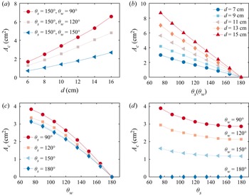
In order to further study the role of the size and the wettability of the container, as shown in figure 16, systematic investigation from different views are carried out. As shown in figure 16(a), for specific values of  $\theta _s$ and
 $\theta _w$,
 $A_c$ increases with
 $d$. When the contact angle of the substrate is fixed, for example,
 $\theta _s = 150^{\circ }$,
 $A_c$ increases with decreasing
 $\theta _w$. As shown in figure 16(b), for the sake of simplicity, let
 $\theta _s = \theta _w$, then we can see that for a fixed value of
 $d$,
 $A_c$ decreases with
 $\theta _s$ (or
 $\theta _w$). Moreover, for a fixed value of
 $\theta _s$ (or
 $\theta _w$),
 $A_c$ increases with
 $d$. Furthermore, as shown in figure 16(c,d), for a specific container diameter (
 $d = 9$ cm), we are able to study the influences of the contact angles of the substrate and the wall. In figure 16(c), we can see that
 $A_c$ decreases with
 $\theta _w$ for each
 $\theta _s$. However, there is no much difference of
 $A_c$ for different values of
 $\theta _s$, especially for larger values of
 $\theta _w$, which is consistent with the conclusions reported by Lv et al. (Reference Lv, Eigenbrod and Hardt2018), where they fixed the contact angle of the wall (
 $\theta _w \approx 90^{\circ }$), but changed the contact angle of the substrate. These results indicate that the influence of
 $\theta _s$ on the instability is of secondary importance. In figure 16(d), we can see that
 $A_c$ decreases with
 $\theta _s$ for each
 $\theta _w$. However, for a fixed value of
 $\theta _s$, the value of
 $A_c$ remarkably changes with
 $\theta _w$, which again demonstrates that
 $\theta _w$ plays a dominant role accounting for the instability of the liquid layer.
Dependency of  $A_c$ on
 $d$,
 $\theta _s$ and
 $\theta _w$. Value of (a)
 $A_c$ as a function of the diameter
 $d$ and (b)
 $A_c$ as a function of the contact angle
 $\theta _s$. Here, we let
 $\theta _s = \theta _w$. Value of (c)
 $A_c$ as a function of the contact angle
 $\theta _w$ with different
 $\theta _s$ and (d)
 $A_c$ as a function of the contact angle
 $\theta _s$ with different
 $\theta _w$. In (c,d), the container diameter is
 $d = 9$ cm.

5. Dynamic behaviour
When  $A$ falls below
 $A_c$, a highly dynamic behaviour sets in, as shown in figure 5. In this section, we discuss the dynamics of the hole collapse in wetting mode II.
To better resolve the final moments of hole collapse, additional experiments were performed with a high time resolution when  $t$ is approaching
 $t_0$. Here,
 $t_0$ stands for the moment when the hole is completely closed. However, accurately determining the value of
 $t_0$ from experiments is very difficult due to the limited frame rate of the high-speed camera. In other words, close to the singularity
 $t_0$, for a single recording, the first frame chosen must have either
 $t>t_0$ or
 $t< t_0$ with
 $\lvert t - t_0 \rvert < \delta t$. Here,
 $\delta t$ represents the time interval between two neighbouring frames (i.e. the first and the second frames), e.g.
 $\delta t = 5 \times 10^{-5} \, \textrm {s}$ when the frame rate is 20 000 frames per second. For a single trial in the practical experiment,
 $t_0$ is determined as the moment captured in the snapshot just prior to the closure of the hole. Subsequently, we obtain the corresponding hole area
 $A$ for
 $(t_0 - t )$. We then repeat the same experiment five times and obtain the average value of these five hole areas to quantify the evolution of the hole area. The time evolution of
 $A$ is shown in figure 17 in a log–log plot. We employed a high-speed camera to capture the final stage of the hole collapse under 20 000 frames per second. We performed experiments with a superhydrophobic substrate (
 $\theta _s = 158.2 \pm 3.0^{\circ }$) and a hydrophobic wall (
 $\theta _w = 116.0 \pm 1.9^{\circ }$). It is noted that the hole collapse predominantly obeys a scaling law
 $A \approx c_1 ( t_0 - t )^{\alpha }$, and a careful analysis reveals that an exponent
 $\alpha = 1.1$ clearly fits better than an exponent of 1 (see supplementary information). The value of the coefficient
 $c_1$ is approximately
 $0.000428 \,\mathrm {m}^2\,\mathrm {s}^{-1.1}$. In contrast to this work, Lv et al. (Reference Lv, Eigenbrod and Hardt2018) selected the diameter
 $d$ to describe the size of the hole and found a scaling law
 $d \sim (t_0 - t )^{0.55}$, which suggested that inertial effects dominate during the hole collapse and the viscosity effects are negligible. Considering
 $A \sim d^2$, our results are consistent with the work of Lv et al. (Reference Lv, Eigenbrod and Hardt2018). Moreover, we can estimate the Reynolds number
 $Re \approx 500$ in our experiment, which reveals that inertial effects dominate and distinguishes our conclusion from Dijksman et al. (Reference Dijksman, Mukhopadhyay, Gaebler, Witelski and Behringer2015) and Bostwick et al. (Reference Bostwick, Dijksman and Shearer2017), where the viscous–capillary effects dominate.
Time evolution of the hole area  $A$ in wetting mode II. Here,
 $t$ is the time and
 $t_0$ is defined as the moment when the hole is completely closed. The red squares are experimental data with error bars, and the black solid line is the best fit to the experimental data based on the scaling law of
 $A \sim (t_0 - t )^{1.1}$.

It is encouraging to compare the hole collapse in our experiment with the final stages of the pinch-off of air bubbles in an inviscid liquid. The latter has been studied quite extensively. Longuet-Higgins, Kerman & Lunde (Reference Longuet-Higgins, Kerman and Lunde1991) established a two-dimensional model to describe the pinch-off dynamics of an air bubble releasing from an underwater nozzle. It is shown that the inertia dominates, while the surface tension, viscosity and the influence of the gas are negligible. A power law  $d \sim t^{0.5}$ for the evolution is reported, which is supported by simulations and experiments (Longuet-Higgins et al. Reference Longuet-Higgins, Kerman and Lunde1991; Oguz & Prosperetti Reference Oguz and Prosperetti1993; Burton, Waldrep & Taborek Reference Burton, Waldrep and Taborek2005). In the experimental work of Thoroddsen, Etoh & Takehara (Reference Thoroddsen, Etoh and Takehara2007), the pinch-off of a bubble in water was studied by employing an ultra-high-speed video imaging and a power-law behaviour
 $d \sim t^{0.57 \pm 0.03}$ was found. Gordillo et al. (Reference Gordillo, Sevilla, Rodríguez-Rodríguez and Martínez-Bazán2005) studied axisymmetric bubble pinch-off in a low-viscosity liquid (e.g. air in water) at high Reynolds numbers, in which the bubble minimum radius (
 $d/2$) decreases as
 $( t_0 - t ) \sim ( d/2 )^2\sqrt {-\ln ( d/2 )^2}$. Eggers et al. (Reference Eggers, Fontelos, Leppinen and Snoeijer2007) studied the collapse of an axisymmetric cavity or bubble inside a fluid of small viscosity, like water, in which the gas inside the cavity and the fluid viscosity are neglected. They reported a scaling law with the exponent very slowly approaching a universal value according to
 $\alpha = 1/2 + 1/[ 4 \sqrt {- \ln ( t_0 - t )} ]$. The variance of the exponent reveals that the dynamics of inviscid bubble pinch-off is not universal, and the exact value depends weakly on initial conditions. The two remaining terms in their equation are inertia, revealing that the inertia effect dominates the dynamics of bubble pinch-off. In agreement with Eggers et al. (Reference Eggers, Fontelos, Leppinen and Snoeijer2007), our results obtained a scaling law
 $A \sim (t_0 - t )^{1.1}$, indicating that the hole collapse in liquid layers is dominated by inertia, and that viscosity can be ignored.
To further confirm the effects of the viscosity, the Ohnesorge number  $Oh = \eta /(\rho \gamma l)^{1/2}$, which relates the viscous forces to inertial and surface tension forces, can be estimated. In our experiment,
 $Oh \approx 1.1 \times 10^{-3}$ in which the material properties of pure water at
 $25^{\,\circ }{\rm C}$ (
 $\eta = 0.891 \times 10^{-3}\,\mathrm {Pa}\,\mathrm {s}$,
 $\rho = 997.1 \,\mathrm {kg}\,\mathrm {m}^{-3}$,
 $\gamma = 0.072\,\mathrm {N}\,\mathrm {m}^{-1}$) were used and
 $l = \sqrt {A_1} = 10$ mm was chosen. Even though the hole shrinks to the typical length
 $l = 0.04$ mm, i.e. the resolution limit of our camera,
 $Oh \approx 1.6 \times 10^{-2}$. These analyses suggest the viscosity effect is negligible.
6. Conclusion
We have presented a combined experimental, numerical and theoretical study of the stability and dynamics of holes at the wall in bounded liquid layers. This study has identified three different wetting modes of holes in liquid layers, depending on the wettabilities of the container. In particular, we found that a hole could maintain stable, could become unstable or could transfer to an inner hole. The first two wetting modes are related to the stability of the holes.
The configuration of the hole is determined by minimizing the energy of the liquid system. In wetting mode I, a stable solution for the liquid–vapour interface exists even for holes with very small areas. In wetting mode II, the evolution of the hole is controlled by a critical value of the hole area below which no stable solution exists. It is found that the critical area increases with increasing container size and decreasing contact angle from the numerical and theoretical results. The contact angle consists of two parts, the wall and the substrate. We found that the relation between  $A_c$ and contact angle would be weak when the contact angle of substrate is large corresponding to the conclusion drawn by Lv et al. (Reference Lv, Eigenbrod and Hardt2018). The phase diagram of different wetting modes is given by employing LBM simulation.
The dynamics of the hole collapse is studied using high-speed imaging techniques. A scaling law  $A \sim t^{1.1}$ is found, indicating that the inertia effect dominates the collapse. The findings reported here have provided a deeper insight into many industrial processes, such as coating, lithography and spraying etc.
However, questions remain. The mechanics behind wetting mode III is still uncertain, especially the interesting dynamic behaviour. Even though we have developed a simple theoretical model and the theoretical results are consistent with the SE and LBM simulation results, however, this model is built based on a uniform thickness of the liquid film, exact solutions of the profile of the liquid film remain unknown. These questions deserve dedicated studies in the future.
Supplementary material and movies
Supplementary material and movies are available at https://doi.org/10.1017/jfm.2023.753.
Acknowledgements
The authors would like to thank K. Li for discussions about SE simulations. The authors are grateful to the anonymous reviewers whose suggestions have helped to significantly improve the paper.
Funding
This work received financial support from the National Natural Science Foundation of China (Grant Nos. 12172189, 52111540269, 11921002, 11902179), and the Tsinghua University Initiative Scientific Research Program (Grant No.20221080070).
Declaration of interests
The authors report no conflict of interest.
Author contributions
H.Z. and B.Z. contributed equally to this work.
Appendix A. Materials and experimental method
The superhydrophobic glass surfaces were prepared by coating the glass plate with silanized silica nanobeads with diameter 30 nm dispersed in isopropanol (Glaco, Soft99) (Vakarelski et al. Reference Vakarelski, Patankar, Marston, Chan and Thoroddsen2012; Dupeux et al. Reference Dupeux, Bourrianne, Magdelaine, Clanet and Quéré2014), which provides water contact angles  $\theta _a = 163.3 \pm 21.0^{\circ }$ and
 $\theta _r = 151.8 \pm 22.4^{\circ }$.
Appendix B. Theoretical model for  ${\theta _w = 180^{\circ }}$

In this appendix, we present theoretical model for  $\theta _w = 180^{\circ }$. Due to its special contact angle
 $\theta _w$, the liquid profile is different from other contact angles (see figure 18). For the sake of simplicity, we choose an approach in which we assume that the liquid film has a uniform thickness.
Simplified liquid layer profile for  $\theta _w = 180^{\circ }$ shown in (a) three-dimensional view and (b) top view.

At a specific time, we assume the liquid has a specific volume  $\varOmega$. The free energy of the system can be written as
 $E=E_s+E_g=A_{lv} \gamma +A_{sl}(\gamma _{sl}-\gamma _{sg})+\rho \varOmega g h / 2$. As shown in figure 18,
 $A_{lv}=A_1+A_2={\rm \pi} r^2 + 2{\rm \pi} r h$,
 $A_{sl}=A_1={\rm \pi} r^2$, thus the free energy can be written as
 \begin{align} E & = E_s+E_g \nonumber\\ & = \left(A_1+A_2\right) \gamma+A_1\left(-\gamma \cos \theta_s\right)+\rho \varOmega g h / 2 \nonumber\\ &= A_1 \gamma\left(1-\cos \theta_s\right)+A_2 \gamma+\rho \varOmega g h / 2. \end{align}
Introducing the radius of the container  $r_1$, we define the dimensionless forms of the relevant geometrical and physical quantities
 \begin{equation} \tilde{r} \equiv \frac{r}{r_1}, \quad \tilde{h} \equiv \frac{h}{r_1}, \quad \tilde{A}_1 \equiv \frac{A_1}{r_1^2}, \quad \tilde{A}_2 \equiv \frac{A_2}{r_1^2}, \quad \tilde{\varOmega} \equiv \frac{\varOmega}{r_1^3}, \quad \tilde{E} \equiv \frac{E}{r_1^2 \gamma}, \end{equation}
and we rewrite (B1) into
 \begin{align} \tilde{E} & = \tilde{A}_1\left ( 1 - \cos \theta_s \right ) + \tilde{A}_2 +\frac{1}{2} \tilde{\varOmega} \tilde{h}\left ( \frac{r_1}{l_c} \right )^{2} \nonumber\\ & = {\rm \pi}\tilde{r}^2 \left ( 1 - \cos \theta_s \right ) + 2{\rm \pi} \tilde{r} \tilde{h} +\frac{1}{2} \tilde{\varOmega} \tilde{h}\left ( \frac{r_1}{l_c} \right )^{2}. \end{align}
In order to obtain the equilibrium profile of the liquid, we minimize the free energy
 \begin{equation} \frac{\partial \tilde{E}}{\partial \tilde{h}}=\frac{\partial\left (\tilde{E}_s+\tilde{E}_g \right ) }{\partial \tilde{h}}=0 ,\end{equation}
and we consider the constraint  $\varOmega =$ constant
 \begin{equation} \frac{\partial \tilde{A}_1}{\partial \tilde{h}}={-}\frac{\tilde{A}_1}{\tilde{h}},\quad \frac{\partial \tilde{r}}{\partial \tilde{h}}={-}\frac{\tilde{r}}{2\tilde{h}}. \end{equation}
Putting (B3) into (B4) and using the relation in (B5a,b)
 \begin{equation} \tilde{h}=\frac{{\rm \pi} \tilde{r}^2\left(1-\cos \theta_s\right)}{\displaystyle {\rm \pi}\tilde{r}+\frac{1}{2} \tilde{\varOmega}\left(\frac{r_1}{l_c}\right)^2}, \end{equation}
and we obtain the equation for  $\theta _w = 180^{\circ }$.
Appendix C. Supplemental curves of theoretical model
To study the influence of the contact angle of substrate and wall on the configuration of the liquid film, we will present more results obtained by the theoretical model in this appendix. As shown in figures 19 and 20, respectively, two cases are studied here based on the theoretical model derived in § 4.1: (i) liquid layers in a circular container with diameter  $d = 9$ cm and contact angle
 $\theta _s = 150^{\circ }$, but with varying contact angles from
 $\theta _w = 60^{\circ }$ to
 $180^{\circ }$; (ii) liquid layers in a circular container with diameter
 $d = 9$ cm and contact angle
 $\theta _w = 90^{\circ }$, but with varying contact angles from
 $\theta _s = 30^{\circ }$ to
 $180^{\circ }$.
Numerical solutions of (4.12) and (4.14) showing (a) the dependence of  $\varOmega$ on
 $A$ and (b) the dependence of
 $E$ on
 $A$. The box size is fixed to
 $d =$ 9 cm, and the contact angle of substrate
 $\theta _s = 150^{\circ }$, while the contact angle of wall varies from
 $\theta _w = 60^{\circ }$ to
 $180^{\circ }$.

Numerical solutions of (4.12) showing (a) the dependence of  $\varOmega$ on
 $A$ and (b) the dependence of
 $E$ on
 $A$. The box size is fixed to
 $d = 9$ cm, and the contact angle of wall
 $\theta _w = 90^{\circ }$, while the contact angle of substrate varies from
 $\theta _s = 30^{\circ }$ to
 $180^{\circ }$.

As shown in figure 19(a), the curves of different  $\theta _w$ collapse at the initial stage. The curves separate until the point of instability, representing different critical values of
 $A_c$. In addition, the shape of
 $\theta _w = 180^{\circ }$ is very different from the others, due to its correspondence to wetting mode I. In other words,
 $\theta _w$ has limited influence on the initial stage, i.e. the stable stage, but it mainly affects the point of instabilities. The instability will happen later when
 $\theta _w$ increases. However, even though liquid films with different
 $\theta _s$ have almost the same area at the initial stage, the effect of
 $\theta _s$ on
 $E$ makes films have different surface energies. Therefore, the curves separate at the initial stage in figure 19(b), but are parallel to each other. The influence of contact angle of substrate
 $\theta _s$ is shown in figure 20. In contrast to figure 19(a), the curves in figure 20(a) do not collapse, but are parallel to each other. The contact angle of the substrate
 $\theta _s$ mainly affects the initial stage of the liquid films, but has little effect on the point of instabilities.