1 Introduction
The flow past a sphere is associated with complex fluid phenomena. It also has a variety of applications. Hence, it has been of continued interest to the fluid mechanics community. The parameter that governs the flow physics is the Reynolds number. It is defined as
 $Re=UD/\unicode[STIX]{x1D708}$
, where
 $D$
is the diameter of the sphere,
 $U$
is the free-stream speed and
 $\unicode[STIX]{x1D708}$
is the kinematic viscosity of the surrounding fluid. The variation of the coefficient of drag acting on the sphere, with
 $Re$
, shows a very significant drop when the boundary layer on the surface of the sphere transitions from a laminar to a turbulent state. This phenomenon is popularly referred to as drag crisis (Landau & Lifshitz Reference Landau and Lifshitz1959; Singh & Mittal Reference Singh and Mittal2005) and has been extensively studied in the past, both numerically and experimentally.
The laminar boundary layer over the surface of a sphere separates near the shoulder due to the adverse pressure gradient. Beyond a critical
 $Re$
, the separated shear layer becomes unstable and rolls up into small vortices that cause a transition to turbulence (Achenbach Reference Achenbach1972; Williamson Reference Williamson1996; Singh & Mittal Reference Singh and Mittal2005). The turbulent shear layer, by virtue of its increased momentum, reattaches onto the sphere surface. The recirculation region formed between the laminar separation and turbulent reattachment is called the laminar separation bubble (LSB). The final flow separation beyond the reattachment of the turbulent boundary layer occurs at a significantly downstream location on the surface of the sphere. The delayed flow separation reduces the size of the wake and increases the base pressure, causing the mean drag coefficient to decrease substantially (Fage Reference Fage1937; Taneda Reference Taneda1978; Suryanarayana & Prabhu Reference Suryanarayana and Prabhu2000; Jeon et al.
Reference Jeon, Choi, Jeon and Choi2004). One of the most comprehensive studies on drag crisis for a smooth sphere was carried out by Achenbach (Reference Achenbach1972). The variation of the mean drag coefficient (
 $\overline{C}_{D}$
) with
 $Re$
was investigated. He classified the entire
 $\overline{C}_{D}$
–
 $Re$
variation into four regimes, namely subcritical, critical, supercritical and transcritical. In the subcritical regime, the boundary layer separates while it is in a laminar state and the flow does not reattach to the surface of the sphere at any downstream location. The mean coefficient of drag is approximately 0.5 throughout this regime and is almost independent of
 $Re$
. Drag crisis is observed in the critical regime, i.e.
 $\overline{C}_{D}$
decreases rapidly with increase in
 $Re$
. In this regime, the boundary layer transitions from a laminar to a turbulent state along with the formation of the LSB. The
 $\overline{C}_{D}$
value increases gradually with increase in
 $Re$
in the supercritical regime. Here, the point of boundary layer transition from laminar to turbulent state remains fixed at a particular azimuthal angle. In the transcritical regime, the upstream shift of the point of boundary layer transition causes an increase in
 $\overline{C}_{D}$
with increase in
 $Re$
.
The phenomenon of drag crisis has also been observed for a bluff body that is nominally two-dimensional, such as a circular cylinder. Previous studies have shown that this phenomenon is very similar for a circular cylinder and sphere (Achenbach Reference Achenbach1971, Reference Achenbach1974). This suggests that the mechanism of the phenomena associated with both these geometries might also be very similar. Schewe (Reference Schewe1983), in his study on the flow past a circular cylinder, classified the flow into three regimes. Unlike Achenbach (Reference Achenbach1972), the classification was based on the nature of variation of the drag force with
 $Re$
, instead of
 $\overline{C}_{D}$
with
 $Re$
. In this classification, the subcritical regime ends and the critical regime begins at the
 $Re$
value where the drag force begins to decrease with increase in
 $Re$
. Similarly, the onset of the supercritical regime and the end of the critical regime occurs at that
 $Re$
where the drag force is minimum. Such a classification results in a sharp boundary between various regimes. The proposal by Achenbach (Reference Achenbach1972) does not lead to such an unambiguous classification, as will be discussed later. In the present work, we extend the classification proposed by Schewe (Reference Schewe1983) for a circular cylinder to the flow past a smooth sphere.
The LSB, which is closely linked with the phenomenon of drag crisis on a sphere/cylinder, has been studied by several researchers in the past. Fage (Reference Fage1937) was amongst the first to observe an LSB on a sphere through surface-pressure measurements. A region of almost constant pressure was utilized to identify the LSB. Achenbach (Reference Achenbach1972) reported the presence of an LSB in the critical flow regime via skin-friction and surface-pressure measurements. Oil flow visualization by Taneda (Reference Taneda1978) at
 $Re\approx 3.5\times 10^{5}$
was used to identify the LSB by accumulation of oil on the surface of the sphere. In their experiments, three distinct lines were observed at azimuthal angles of
 $100^{\circ }$
,
 $117^{\circ }$
and
 $135^{\circ }$
from the stagnation point. These were identified as the approximate locations for laminar separation, turbulent reattachment and the final turbulent separation, respectively. The presence of the LSB between the lines at
 $100^{\circ }$
and
 $117^{\circ }$
was confirmed by the reverse flow in this region. Suryanarayana & Prabhu (Reference Suryanarayana and Prabhu2000) also observed the LSB for the critical flow over an unvented sphere through oil flow visualization and compared their flow separation and reattachment angles with those reported earlier. They also reported the existence of an LSB in the early supercritical regime, at
 $Re\approx 6.5\times 10^{5}$
.
Singh & Mittal (Reference Singh and Mittal2005) carried out two-dimensional simulations across the critical flow regime to investigate the mechanism of drag crisis for a circular cylinder. They found that the separated shear layer, following the separation of the boundary layer from the surface of the cylinder, becomes unstable at a downstream location and rolls up into shear layer vortices. The location of the onset of the instability of the shear layer moves upstream with increase in
 $Re$
. At the critical
 $Re$
, this location moves very close to the surface of the cylinder. The shear layer vortices impart momentum to the separated flow near the surface of the cylinder, causing it to reattach. Consequently, an LSB is formed between the point of boundary layer separation and the flow reattachment. It appears that for both the sphere (Achenbach Reference Achenbach1972) and the cylinder (Singh & Mittal Reference Singh and Mittal2005), the onset of the drag crisis is associated with the formation of an LSB. This is explored in detail in the present work for the flow past a sphere.
One question that naturally arises is: Does the LSB suddenly appear at a certain
 $Re$
as
 $Re$
is increased? To the best of our knowledge, for the case of flow over a sphere, this has not been explored in detail in the past. One reason may be that simple time averaging of flow may not yield the physics of the formation of the LSB. There are very few studies that have investigated the unsteady dynamics of the LSB in the past. Miau et al. (Reference Miau, Tsai, Lin, Tu, Fang and Chen2011), via surface-pressure measurements, presented a thorough study on the unsteady flow behaviour for flow past a smooth circular cylinder in the regime of the boundary layer transition. During the transition from the subcritical to critical regime, they observed significant pressure fluctuations near the shoulder of the cylinder. These were attributed to the unsteadiness involved with the laminar flow separation along with the gradual development of a separation bubble. At slightly higher
 $Re$
in the critical flow regime, high-pressure fluctuations were observed in the region of turbulent flow reattachment on the cylinder. These were attributed to the highly unsteady nature of the reattached turbulent flow. Interestingly, at these
 $Re$
, the pressure fluctuations in the region near the laminar flow separation were relatively low. This suggests the stable nature of the LSB at higher
 $Re$
in the critical regime. Cadot et al. (Reference Cadot, Desai, Mittal, Saxena and Chandra2015), in their study on the dynamics of the boundary layer reattachment for a circular cylinder, made similar observations about the increased unsteadiness near the region of turbulent flow reattachment. Recently, Chopra & Mittal (Reference Chopra and Mittal2017) presented a numerical study that explored the mechanism of drag crisis for the flow past a circular cylinder. They found that the LSB is intermittent in the critical flow regime. Through statistical analysis of the surface pressure, they showed that the frequency of appearance of the LSB and the duration of its stay increase with increase in
 $Re$
in the critical regime. The LSB exists at all times for
 $Re$
beyond the critical regime.
Earlier studies have shown that the unsteady dynamics associated with the LSB is also reflected in the time histories of the fluid forces on the body. For example, according to the results of Schewe (Reference Schewe1983), the lift fluctuations for the critical flow past a circular cylinder show broad-band ‘critical fluctuations’ at low frequency in addition to a peak at the vortex shedding frequency. These critical fluctuations were attributed to the random switching of the flow between the subcritical and supercritical flow states. The fluctuations were observed to be most prominent in the early stages of the critical regime and diminished by the end of the critical regime. A similar observation was made by Norman & McKeon (Reference Norman and McKeon2011) for the flow past a smooth sphere. They reported an intermittent switching of the instantaneous drag force between values that correspond to subcritical and supercritical states. This behaviour is evident in their probability density plot of the drag coefficient measured in the critical regime, where
 $C_{D}$
shows a bimodal distribution.
Despite the large number of studies that have been reported in the past for the critical flow past a smooth sphere, the dynamics of the formation of the LSB is still not completely understood. In the present work we attempt to address the following questions. (i) Does the LSB appear suddenly at a certain
 $Re$
in the critical regime? Or, does it appear intermittently at an initial
 $Re$
in the critical regime and then achieve a more permanent status at a higher
 $Re$
? (ii) If the LSB is indeed intermittent at the onset of its formation, does the intermittency in the LSB exist throughout the critical flow regime, or is it restricted to a certain range of
 $Re$
within the critical regime? (iii) During its intermittent appearance, do the appearance and disappearance of the LSB happen simultaneously at all circumferential locations at a certain azimuthal angle on the surface of the sphere? (iv) We observe that
 $\overline{C}_{D}$
decreases with increase in
 $Re$
in the critical flow regime. Does this variation have any relation with the occurrence of the LSB in this regime? To answer these questions, experimental investigations are carried out on the flow past a smooth sphere for
 $1.5\times 10^{5}\leqslant Re\leqslant 5.0\times 10^{5}$
. Unsteady force, surface-pressure measurements and hot-wire anemometry are used to explore the flow dynamics. We extend the concept of an intermittency factor (
 $I_{f}$
), which is extensively used to quantitatively define the extent of flow transition from a laminar to a turbulent state (Tennekes & Lumley Reference Tennekes and Lumley1972), to the present study. We utilize it to provide a quantitative estimation of the intermittent occurrence of the LSB over the sphere.
2 Experimental set-up
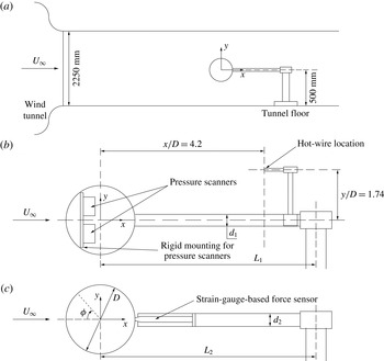
Figure 1 shows the schematic of the experimental set-up. The experiments were conducted in a closed-circuit suction-type atmospheric wind tunnel with a test section size of
 $3~\text{m}\times 2.25~\text{m}$
. The maximum achievable wind speed in the test section is
 $80~\text{m}~\text{s}^{-1}$
. The maximum spatial inhomogeneity of the incoming flow was measured to be 0.05 % approximately at a speed of
 $20~\text{m}~\text{s}^{-1}$
. The turbulence intensity in the tunnel test section was measured to be below 0.06 % throughout the operating speed range of the tunnel. The measurements in the present study were carried out in the velocity range
 $20{-}66~\text{m}~\text{s}^{-1}$
. More details on the characterization of the wind tunnel can be found in the article by Cadot et al. (Reference Cadot, Desai, Mittal, Saxena and Chandra2015).
(a) Schematic of the model mounting in the tunnel test section (dimensions are in millimetres) along with the coordinate axes. Experimental set-up for (b) pressure and (c) force measurements.

A schematic of the mounting of the sphere model is also shown in figure 1. The diameter
 $D$
of the sphere is 120 mm. The blockage ratio of the cross-sectional area of the sphere to the area of the test section is 0.16 % approximately. The model is fabricated using stereo-lithography rapid prototyping technique with Accura SI 60 resin material. Following the fabrication, the sphere had a surface finish of
 $k/D\approx 66.67\times 10^{-5}$
. A paint with matte finish was applied to the model to further improve its surface finish. The model is an assembly of two hollow pieces which join together at an azimuthal angle of
 $\unicode[STIX]{x1D719}=130^{\circ }$
from the front stagnation point. This ensures that the seam appearing due to the assembly of the two parts is located away from the region of the transition boundary layer. Therefore, it is expected to have no significant influence on the flow. As shown in figure 1(b,c), two different stings were utilized to support the model. This was done to cater for the differing instrumentation requirements for the force and surface-pressure measurements. The support sting for the force measurement experiments was made from a hollow stainless-steel pipe, with an outer diameter of 25 mm
 $(d_{2})$
and length of 480 mm
 $(L_{2})$
. This arrangement allowed the force sensor to be firmly mounted immediately downstream of the sphere. For the pressure measurements, the sphere was supported at the rear by a different hollow sting of stainless steel with outer diameter 21 mm
 $(d_{1})$
and length of 650 mm
 $(L_{1})$
. The sting diameter was required to be large in this case as well to allow the passage of power supply cables of the pressure scanner installed inside the sphere. The ratio of the diameter of the sting to that of the sphere for the two support stings is 0.21 and 0.175. This is well below the maximum limit of 0.25 suggested by Norman & McKeon (Reference Norman and McKeon2008) to be appropriate for studying the flow past a sphere in the subcritical regime. Further, to prevent the sphere from vibrating, the rear horizontal sting was fixed to a rigid vertical support, which in turn was anchored to the ground of the test section.
The unsteady forces on the sphere were measured using a six-component strain-gauge-based force sensor. This sensor was installed inside the horizontal sting supporting the sphere such that the head of the sensor was directly connected to the downstream end of the sphere (figure 1
c). A similar set-up was used by Suryanarayana, Pauer & Meier (Reference Suryanarayana, Pauer and Meier1993), where the force-measuring sensor was installed on the sting holding the sphere. The calibration curve obtained for the sensor is linear. The non-dimensional force components along the three Cartesian directions are denoted by
 $C_{D}$
,
 $C_{Y}$
and
 $C_{Z}$
. The maximum uncertainty in
 $\overline{C}_{D}$
measurement is
 $\pm 1.52\,\%$
at
 $Re=1.5\times 10^{5}$
. The output from the balance was amplified and sampled for 60 s at an acquisition rate of 500 Hz to obtain the time-series data. Thus, at the lowest velocity of
 $20~\text{m}~\text{s}^{-1}$
, the non-dimensional time unit for which the data were acquired is
 $tU_{\infty }/D=10^{4}$
. This is well above the
 $tU_{\infty }/D\approx 2000$
suggested by Norman & McKeon (Reference Norman and McKeon2011) to adequately capture the dynamics of high-
 $Re$
flow past a sphere. In a selective
 $Re$
range in the critical flow regime, where the drag force was observed to be intermittent between two states, force measurement was carried out for a longer duration of 300 s. At each
 $Re$
in the range
 $1.5\times 10^{5}\leqslant Re\leqslant 5.0\times 10^{5}$
, the force measurements were repeated at least twice. The results from the three runs are in excellent agreement.
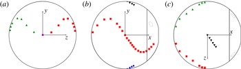
Schematic of the model of a smooth sphere with pressure ports arranged along four splines: A (▪), B (♦), C (▴) and D (▾). The flow is along the positive
 $x$
direction and the front stagnation point is shown in (a) by a solid circle (●). The size and number of ports shown in the figure are only representative. Not all ports have been shown, to avoid clutter.

The static pressure distribution on the surface of the sphere was recorded via 63 pressure taps. The holes for the pressure taps were drilled normal to the surface of the sphere and arranged along splines to avoid interference between the various pressure ports. Figure 2 shows the distribution of these taps on the surface of the model. This arrangement of ports gives us the variation of surface pressure in the azimuthal direction. In addition, four pressure ports were provided on the sting, in the portion close to the
 $\unicode[STIX]{x1D719}=180^{\circ }$
region of the sphere, to measure the back-pressure. The back-pressure reported in this article is the average of these four ports. A total of 62 pressure ports on the surface of the sphere are distributed along the splines A–D (figure 2). Of these, 25 ports are distributed along each of the two splines A and C, while six ports lie on each of the two splines B and D. One pressure port is located at the front stagnation point, at
 $\unicode[STIX]{x1D719}=0^{\circ }$
. Along splines A and C, the ports are located in the range
 $15^{\circ }\leqslant \unicode[STIX]{x1D719}\leqslant 150^{\circ }$
. Of these, 13 are located in the region
 $90^{\circ }\leqslant \unicode[STIX]{x1D719}\leqslant 126^{\circ }$
to capture the LSB. The ports on splines B and D are equally spaced in the range
 $90^{\circ }\leqslant \unicode[STIX]{x1D719}\leqslant 105^{\circ }$
. A total of three ESP scanners were used for the present study, each having an operational range of
 $-2500$
to
 $+2500~\text{Pa}$
. Of these, two ESP scanners were installed and firmly held with a support provided inside the sphere (figure 1
b). They were used to acquire the instantaneous pressure data from the ports on the sphere surface. One scanner was kept outside the tunnel to acquire the pressure data from the back-pressure ports, static pressure and total pressure in the tunnel. The resolution of the pressure transducer is
 $\pm 0.05\,\%$
of 2500 Pa. The output signal was sampled for 120 s with an acquisition rate of 500 Hz per pressure port. The frequency of intermittent switching between the flow states of interest, in this work, is found to be relatively small. The smallest time period of switching is of the order of a second. The response time of the sensor is less than 4 ms. Therefore, the dynamic response of the ESP scanners is sufficiently fast to capture the corresponding change in the surface pressure. More details on the response characteristics of the sensor can be found in the article by Solliec & Mary (Reference Solliec and Mary1995). The frequency response of the pressure measurement system may be adversely affected by an increase in the length of the tubing connecting the pressure taps on the model to the pressure scanner. The ESP scanners, which are connected to the pressure taps to measure the surface pressure, are installed inside the sphere in the present set-up. Consequently, the length of the pressure tubing is very small and is expected to have no significant effect on the frequency response of the measurement system.
An independent run was also carried out in the
 $Re$
range where an intermittent nature of the drag force was observed. In this test, surface-pressure measurements and hot-wire anemometry were carried out simultaneously and data were acquired for 300 s, similar to force measurements. Owing to limitations in the available instrumentation, force and surface-pressure measurements could not be carried out simultaneously. With the drag crisis phenomenon being extremely sensitive to the set-up, it occurred at a slightly larger
 $Re$
during pressure measurement experiments as compared to that during force measurements. To be able to correlate force and pressure data, the pressure measurements are reported at a modified
 $Re$
. The offset is
 $\unicode[STIX]{x0394}Re\approx 5300$
from the original measurements. The offset value is rather insignificant compared to the
 $Re$
range (
 $3.4\times 10^{5}<Re<4.4\times 10^{5}$
) of the critical flow regime.
A platinum-plated tungsten wire, soldered to the prongs, was used for hot-wire anemometry. The wire is
 $5~\unicode[STIX]{x03BC}\text{m}$
in diameter and 1.25 mm in length. At an overheat ratio of 0.8, the cutoff frequency of the sensor was 10 kHz approximately. The voltage readings from the anemometer were calibrated with the free-stream speed using a standard two-hole Pitot tube and a digital manometer. A power-law fit was used to fit the voltage versus velocity curve. The output from the hot-wire sensor was digitized using a 16-bit analog-to-digital board, resulting in a resolution of 0.076 mV. The smallest change in the velocity that can be detected by the sensor is of the order of
 $0.01~\text{m}~\text{s}^{-1}$
. The hot-wire signals were sampled at a rate of 500 Hz for 300 s. After the calibration in the desired speed range is carried out, the uncertainty in the velocity measurement is less than 1.0 %. The hot-wire probe was positioned in the direction of the flow on the rear horizontal sting at a distance of
 $x/D=4.2$
and
 $y/D=1.74$
from the centre of the sphere. This location was chosen to capture the separated shear layer activity following the laminar boundary layer separation from the sphere (Kim & Durbin Reference Kim and Durbin1988).
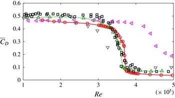
Variation of the mean drag coefficient with
 $Re$
: ○, present study; ▫, Achenbach (Reference Achenbach1972); ▵, Norman, Kerrigan & McKeon (Reference Norman, Kerrigan and McKeon2011); ▿, Wieselsberger (Reference Wieselsberger1922); ◃, Suryanarayana et al. (Reference Suryanarayana, Pauer and Meier1993).

Surface oil flow visualization, using a mixture of paraffin oil and titanium dioxide, was carried out on a model of a sphere that has the same diameter as that used for pressure and force measurements, but is devoid of pressure ports. The same manufacturing process is utilized to fabricate the two models so that their surface roughnesses are as close as possible. A camera was installed outside the tunnel. It captures pictures in the
 $x$
–
 $z$
plane. The
 $x$
–
 $z$
plane being parallel to the tunnel floor ensured that there would be no influence of gravity on the surface oil flow patterns. The experiment was conducted in the following manner. First, the mixture for visualization was uniformly applied to the surface of the model with a brush. Immediately thereafter, the fan of the tunnel was turned on and the wind flow is allowed to achieve the desired speed. The wind speed is maintained for sufficient time to permit the oil flow on the surface of the model to equilibrate with the flow of the air. This is ensured by examining a video of the oil flow on the model surface during this period. Once it is established that the oil pattern has achieved a steady state, final images of the model with the oil pattern were captured. The tunnel speed was later brought back to zero so that the oil mixture could be applied again for visualizing the flow pattern for the next flow speed.
3 Results
3.1 Variation of drag and lateral forces
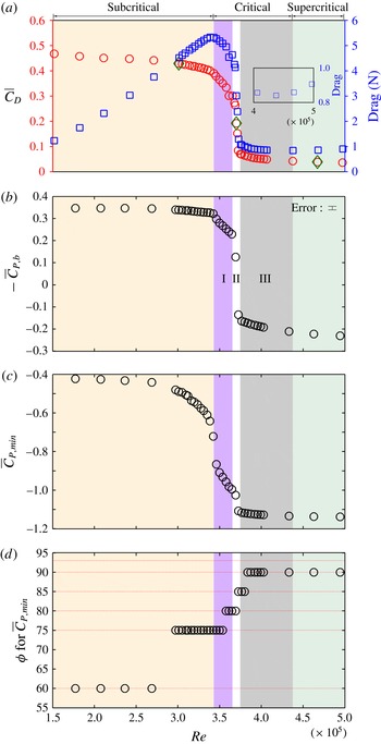
Figure 3 shows the variation of the mean drag coefficient
 $\overline{C}_{D}$
obtained in the present study with
 $Re$
. Also shown is the variation from earlier studies. In the subcritical
 $Re$
regime,
 $\overline{C}_{D}$
for the present study matches reasonably well with results of Wieselsberger (Reference Wieselsberger1922) and Suryanarayana et al. (Reference Suryanarayana, Pauer and Meier1993). However, these values are slightly lower than the measurements of Achenbach (Reference Achenbach1972) and Norman et al. (Reference Norman, Kerrigan and McKeon2011). The difference in the results from the various studies might be due to the difference in the experimental set-ups. The experimental set-up used in the present study is very similar to that used by Suryanarayana et al. (Reference Suryanarayana, Pauer and Meier1993). In both the studies, the force-measuring sensor was installed on the sting that holds the sphere. On the other hand, in the studies by Achenbach (Reference Achenbach1972) and Norman et al. (Reference Norman, Kerrigan and McKeon2011), the force sensor was installed inside the sphere. In the supercritical regime,
 $\overline{C}_{D}$
measured in the present study is slightly lower than that reported by others. This difference can be attributed to the higher sting-to-sphere diameter ratio
 $(d_{2}/D)$
for our experimental set-up compared to that of others. Hoerner (Reference Hoerner1935) investigated the effect of this ratio on the drag coefficient. He found that it does not have a significant effect on
 $\overline{C}_{D}$
in the subcritical regime but can change
 $\overline{C}_{D}$
significantly in the supercritical regime. It was shown that an increase in this ratio leads to a decrease in
 $\overline{C}_{D}$
in the supercritical regime. Despite the presence of pressure ports on the surface of the model of sphere, the drag crisis in the present study occurs at a slightly higher
 $Re$
as compared to that observed in earlier studies. This difference is attributed to the relatively low turbulence level of the present wind tunnel compared to the tunnels used in earlier studies.
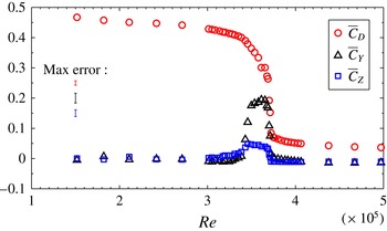
Figure 4 depicts the variation of the coefficients of three components of force along the three axes with
 $Re$
. The estimate of the maximum error for each force coefficient is also indicated. The lateral force coefficients are labelled as
 $C_{Y}$
and
 $C_{Z}$
in accordance with figure 1. The values of
 $C_{Y}$
and
 $C_{Z}$
are negligible in the subcritical and supercritical regime but are significant in the critical flow regime. Non-zero lateral forces in the critical flow regime were also reported by Norman & McKeon (Reference Norman and McKeon2011). They attributed these to minute manufacturing imperfections on the surface of the sphere. These imperfections result in an earlier transition of the boundary layer over a particular region of the sphere, resulting in a non-axisymmetric flow separation from the surface. As
 $Re$
approaches the end of the critical regime, the flow transition nears completion throughout the sphere surface, due to which the lateral force coefficients decrease in magnitude. In order to check for a bias in the lateral plane, force measurements were also carried out after rotating the sphere about the free-stream axis at several angles. In each case, even though the magnitude of
 $\overline{C}_{Y}$
and
 $\overline{C}_{Z}$
changed on rotation, the resultant lateral force coefficient remained the same at a particular
 $Re$
, irrespective of the rotation angle.
Variation of the coefficients of three components of force with
 $Re$
. Also shown is the estimate of maximum error.

Variation with
 $Re$
of: (a)
 $\overline{C}_{D}$
and mean drag force; (b) time-averaged base pressure coefficient,
 $-\overline{C}_{P,b}$
; (c) the minimum time-averaged pressure coefficient,
 $\overline{C}_{P,min}$
measured on the surface of the sphere on spline A; and (d) its angular location
 $\unicode[STIX]{x1D719}$
. For a few values of
 $Re$
, as highlighted in panel (a) by green diamonds, the time variation of
 $C_{D}$
is shown in figure 6. In panel (d), the azimuthal location of pressure ports is also indicated by broken horizontal lines. The various flow regimes as well as subregimes are also marked.

3.2 Classification of flow regimes
Figure 5(a) depicts the variation of the time-averaged drag coefficient with
 $Re$
. The variation in the drag force is also shown in the same panel. Achenbach (Reference Achenbach1972) classified the flow past a sphere into various regimes on the basis of variation of
 $\overline{C}_{D}$
with
 $Re$
. Later, Schewe (Reference Schewe1983), for flow past a circular cylinder, proposed a classification of the various regimes on the basis of variation of drag force with
 $Re$
. As the identification of the flow regimes is relatively easier and virtually unambiguous with the latter approach, in the present work, we extend the proposal by Schewe (Reference Schewe1983) to the flow past a sphere. The flow regimes, namely subcritical, critical and supercritical, are marked in figure 5. In the subcritical flow regime, the drag force increases with
 $Re$
. On the other hand,
 $\overline{C}_{D}$
shows a gradual decrease with
 $Re$
. The decrease is more significant in the higher subcritical regime (
 $2.5\times 10^{5}<Re<3.4\times 10^{5}$
). A similar decrease in
 $\overline{C}_{D}$
, in the higher subcritical regime, can be observed in figure 3 in Norman et al. (Reference Norman, Kerrigan and McKeon2011). We now try to explore the reason for this decrease. The variation of
 $\overline{C}_{D}$
with
 $Re$
has been previously shown to have a good correlation with the variation of base pressure with
 $Re$
(Williamson Reference Williamson1996). Hence, we show the variation of the base suction coefficient,
 $-\overline{C}_{P,b}$
, with
 $Re$
in figure 5(b). It can be noted that the decrease in
 $-\overline{C}_{P,b}$
with
 $Re$
is too small to explain the decrease in
 $\overline{C}_{D}$
in the subcritical regime. Therefore, we explore alternative mechanisms. Figure 5(c,d) shows the variation of the minimum pressure (i.e. maximum suction) on the surface of the sphere (spline A), and its azimuthal location with
 $Re$
. The maximum suction on the sphere increases significantly in the higher subcritical regime. More importantly, this suction is located relatively away from the shoulder (
 $\unicode[STIX]{x1D719}\approx 75^{\circ }$
). Hence, an increase in suction contributes to a reduction in
 $\overline{C}_{D}$
. From this, we conclude that the decrease in
 $\overline{C}_{D}$
, with increase in
 $Re$
, in the higher subcritical regime is not caused by an increase in base pressure. Rather, it can be attributed to the increase in the suction upstream of the shoulder of the sphere.
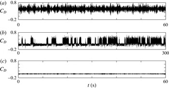
Time history of
 $C_{D}$
at three
 $Re$
: (a)
 $Re=3.01\times 10^{5}$
, (b)
 $Re=3.70\times 10^{5}$
and (c)
 $Re=4.67\times 10^{5}$
. These values of
 $Re$
belong to the subcritical, critical and supercritical regimes, respectively, and are marked in figure 5(a).

Schewe (Reference Schewe1983), for the flow past a cylinder, proposed that the critical regime is characterized by a decrease in the time-averaged drag force with an increase in
 $Re$
. When applied to the data for flow past a sphere from the present study, the critical regime is found to be
 $3.4\times 10^{5}<Re<4.4\times 10^{5}$
. It is evident from figure 5 that the critical regime is very rich in terms of the flow phenomena. We utilize the variation of the base suction coefficient with
 $Re$
to further subdivide the critical regime into three subregimes, as marked in figure 5. In subregimes I and III,
 $-\overline{C}_{P,b}$
decreases gradually with increase in
 $Re$
. In subregime II, it experiences a near jump at
 $Re\approx 3.7\times 10^{5}$
, including a change in its sign. Later in the paper, we will show that the flow exhibits significant differences in these subregimes with respect to the LSB.
The minimum pressure coefficient and its location at various
 $Re$
are shown in figure 5(c,d). In subregime I, both
 $-\overline{C}_{P,b}$
and
 $\overline{C}_{P,min}$
decrease with increase in
 $Re$
. Hence, both these effects contribute to the decrease in the drag coefficient with increase in
 $Re$
in this subregime. In subregimes II and III, the decrease in
 $\overline{C}_{D}$
with increase in
 $Re$
is due to the increase in the time-averaged base pressure coefficient. Although the peak suction near the shoulder also increases with
 $Re$
in these subregimes, its contribution to the decrease in drag is insignificant. Specifically, in subregime III, the peak suction saturates at
 $\overline{C}_{P,min}\approx -1.13$
and is located at
 $\unicode[STIX]{x1D719}\approx 90^{\circ }$
. The time-averaged drag force increases with increase in
 $Re$
beyond
 $Re\approx 4.4\times 10^{5}$
. This is a characteristic of the supercritical regime (Schewe Reference Schewe1983). Even though the drag force increases,
 $\overline{C}_{D}$
continues to decrease with
 $Re$
, although very gradually, up to
 $Re=5.0\times 10^{5}$
investigated in the study. This decrease in
 $\overline{C}_{D}$
is due to the gradual increase in the base pressure coefficient.
To further bring out the difference in the three regimes, we consider the time series of the drag coefficient at an
 $Re$
from each of the three regimes. These
 $Re$
are identified in figure 5(a) and the corresponding time histories at these
 $Re$
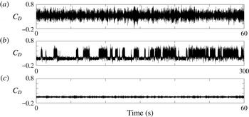
are shown in figure 6. At
 $Re=3.01\times 10^{5}$
(subcritical regime) in figure 6(a), the drag coefficient varies about
 $\overline{C}_{D}\approx 0.43$
, with a dominant frequency that corresponds to a Strouhal number,
 $St\approx 0.17$
(
 $St$
is the non-dimensional frequency normalized with free-stream speed and the diameter of the sphere). The time history at
 $Re=3.70\times 10^{5}$
, shown in figure 6(b) for the critical regime, displays an intermittent transition between bistable states. The mean values of
 $C_{D}$
for the two states are 0.29 and 0.08. Further, the time variation in
 $C_{D}$
exhibits significantly larger variation about the state with larger mean as opposed to the one with lower mean. The larger variation is comparable to that observed in the subcritical regime. In the supercritical regime, as shown in figure 6(c) at
 $Re=4.67\times 10^{5}$
,
 $C_{D}$
varies about a mean value of
 $\overline{C}_{D}\approx 0.04$
with relatively low-amplitude variation. To further investigate the intermittent variation in
 $C_{D}$
in the critical flow regime, surface-pressure measurements were carried out at various
 $Re$
. These results are presented in the following section.
3.3 Laminar separation bubble
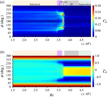
Figure 7 shows the angular distribution of the root-mean-square (r.m.s.) and time-averaged pressure coefficients (
 $C_{P}^{\prime }$
and
 $\overline{C}_{P}$
, respectively) with
 $Re$
. The pressure data presented in figure 7 and later in the paper utilize the pressure ports that lie on spline A (figure 2) for
 $0^{\circ }\leqslant \unicode[STIX]{x1D719}\leqslant 180^{\circ }$
and those that lie on spline C for
 $180^{\circ }\leqslant \unicode[STIX]{x1D719}\leqslant 360^{\circ }$
. Barring the critical flow regime, it is evident from figure 7(b) that the pressure distribution is fairly symmetric about
 $\unicode[STIX]{x1D719}=180^{\circ }$
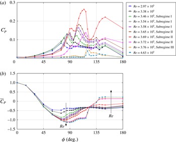
. The asymmetry in the critical regime is expected because the flow transitions in this regime are quite sensitive to the slightest manufacturing imperfections. These are also responsible for the non-zero lateral forces in the critical regime, as shown in figure 4. In order to highlight certain specific features in the pressure distribution plotted in figure 7, figure 8(a,b) shows the line plots of
 $C_{P}^{\prime }$
and
 $\overline{C}_{P}$
at certain
 $Re$
for
 $0^{\circ }\leqslant \unicode[STIX]{x1D719}\leqslant 180^{\circ }$
.
The variation of (a) r.m.s. and (b) mean coefficients of pressure on the
 $\unicode[STIX]{x1D719}$
–
 $Re$
plane.

As shown in the previous section, the maximum suction on the surface of the sphere increases and shifts downstream with increase in
 $Re$
in the higher subcritical regime. The line plots in figure 8(b) for
 $Re=2.97\times 10^{5}$
and
 $3.38\times 10^{5}$
as well as figure 7(b) clearly depict this behaviour. In this regime, the time-averaged azimuthal angle corresponding to the separation of the laminar boundary layer from the surface of the sphere is approximately
 $82^{\circ }$
(Achenbach Reference Achenbach1972). At each
 $Re$
, the point of separation moves along the surface of the sphere with time, leading to unsteadiness in the pressure distribution. The
 $C_{P}^{\prime }$
distribution is associated with two peaks, as also reported in earlier studies (Miau et al.
Reference Miau, Tsai, Lin, Tu, Fang and Chen2011; Cadot et al.
Reference Cadot, Desai, Mittal, Saxena and Chandra2015). The main peak in
 $C_{P}^{\prime }$
(figures 7
a and 8
a) gradually moves downstream with increase in
 $Re$
. This shift in the peak of unsteadiness suggests a gradual delay in the flow separation as the flow approaches a critical state.
Angular distribution of (a) r.m.s. (
 $C_{P}^{\prime }$
) and (b) time-averaged (
 $\overline{C}_{P}$
) pressure coefficients at various
 $Re$
. Curves for
 $Re$
in the subcritical, critical and supercritical regimes are represented by dashed, solid and dash-dotted lines, respectively.

The critical regime (
 $3.4\times 10^{5}<Re<4.4\times 10^{5}$
) is further subdivided into three regions. These are also marked in figure 7(a,b). Increased unsteady activity for
 $85^{\circ }<\unicode[STIX]{x1D719}<115^{\circ }$
(figure 7
a) is manifested in the
 $C_{P}^{\prime }$
distribution in subregime I (
 $3.4\times 10^{5}<Re<3.65\times 10^{5}$
). The corresponding line plots shown in figure 8(a) depict two peaks in the azimuthal variation of
 $C_{P}^{\prime }$
. The peak values increase and move downstream with increase in
 $Re$
. The movement of the peak pressure fluctuations with
 $Re$
represent the delay in laminar flow separation (Miau et al.
Reference Miau, Tsai, Lin, Tu, Fang and Chen2011). The maximum suction on the sphere increases and shifts closer to the shoulder of the sphere with increase in
 $Re$
(figures 7
b and 8
b). Subregime II (
 $3.65\times 10^{5}<Re<3.75\times 10^{5}$
) is characterized by the appearance of a plateau in
 $\overline{C}_{P}$
downstream of the shoulder of the sphere. It becomes quite prominent close to the end of subregime II, as shown in figure 8(b) for
 $Re=3.72\times 10^{5}$
. A pressure plateau in this azimuthal angle range suggests the development of an LSB, as reported in earlier studies (Suryanarayana & Meier Reference Suryanarayana and Meier1995). The unsteady separation of the laminar boundary layer and the turbulent reattachment lead to two fairly large peaks in the distribution of
 $C_{P}^{\prime }$
. At
 $Re=3.69\times 10^{5}$
, these peaks are located at
 $\unicode[STIX]{x1D719}\approx 93^{\circ }$
and
 $117^{\circ }$
, approximately. Hence, an LSB exists between these two values of
 $\unicode[STIX]{x1D719}$
. This phenomenon has also been reported earlier by Achenbach (Reference Achenbach1972) and Taneda (Reference Taneda1978). The variation of
 $\overline{C}_{P}$
and
 $C_{P}^{\prime }$
distributions with
 $Re$
suggests that subregime II is associated with the development of an LSB. The LSB is very weak at the onset of subregime II and is fairly well developed at the end of this subregime. Another observation that suggests the development of an LSB in subregime II is the significant fluctuation in the back-pressure coefficient in this subregime as compared to the other two subregimes. Subregime III (
 $3.75\times 10^{5}<Re<4.4\times 10^{5}$
) is associated with a fully developed LSB as seen from figures 7(b) and 8(b). The constant pressure plateau, which exists for
 $105^{\circ }<\unicode[STIX]{x1D719}<120^{\circ }$
, indicates the approximate azimuthal locations for laminar separation (
 $\unicode[STIX]{x1D719}\approx 105^{\circ }$
) and turbulent reattachment (
 $\unicode[STIX]{x1D719}\approx 120^{\circ }$
). This is further confirmed by a single peak in
 $C_{P}^{\prime }$
at
 $\unicode[STIX]{x1D719}\approx 120^{\circ }$
, which corresponds to the turbulent reattachment of the boundary layer (Miau et al.
Reference Miau, Tsai, Lin, Tu, Fang and Chen2011). The reattachment of the turbulent shear layer is associated with pressure recovery on the surface of the sphere downstream of the shoulder. The turbulent boundary layer eventually separates at
 $\unicode[STIX]{x1D719}\approx 135^{\circ }$
, which is indicated by the constant pressure distribution on the aft side of the sphere. Compared to subregime II, the biggest change in this subregime is the base pressure, as well as the region of suction downstream of the shoulder of the sphere. To summarize, the surface-pressure measurements show that the critical regime consists of three subregimes. Subregime I is devoid of an LSB, while subregime II is associated with the onset and development of the LSB. In this subregime, the LSB is intermittent in nature. This is consistent with the bistable variation of
 $C_{D}$
(figure 6
b) in this subregime. Finally, subregime III is associated with a fully developed LSB.
There are several similarities in the azimuthal location of the various flow phenomena between the supercritical regime and subregime III. For example, the locations of the laminar separation, turbulent reattachment and turbulent separation of the boundary layer are approximately the same in the two cases. This is evidenced by the constant pressure distribution on the surface of the sphere, associated with the LSB and with the turbulent separation on the aft side of the sphere.
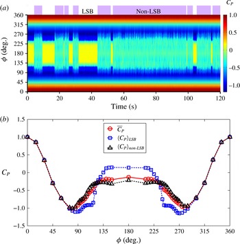
(a) Space–time diagram of the pressure coefficient on the surface of the sphere at
 $Re=3.69\times 10^{5}$
depicting the LSB and non-LSB states. (b) Angular distribution of the conditional time-averaged pressure coefficient at the same
 $Re$
. The red circles represent the time-averaged
 $C_{P}$
, the blue squares represent the conditional time-averaged
 $C_{P}$
for the LSB state and the black triangles represent the conditional time-averaged
 $C_{P}$
for the non-LSB state.

3.4 Intermittent nature of the laminar separation bubble
To further explore the intermittent nature of the LSB in subregime II of the critical regime, we examine the time histories of certain quantities. Figure 9(a) shows the space–time diagram of the
 $C_{P}$
distribution for
 $Re=3.69\times 10^{5}$
. The time instants at which an LSB exists are associated with relatively large base pressure (
 $\overline{C}_{P,b}$
) compared to the time instants when an LSB does not exist. Hence, we utilize the base pressure coefficient to identify the LSB and non-LSB states at different time instants. A threshold value of
 $C_{P,b}$
was identified. When the back-pressure coefficient is above this value, the flow at this time instant corresponds to the LSB state. At other times, when
 $C_{P,b}$
is lower than the threshold value, the flow is in a non-LSB state. The LSB and non-LSB states have been marked in figure 9(a). Figure 9(b) shows the
 $\overline{C}_{P}$
as well as the conditional time-averaged
 $C_{P}$
distribution for these two states. The plateau in
 $C_{P}$
distribution, characteristic of an LSB, is clearly visible in
 $\langle C_{P}\rangle _{LSB}$
(time-averaged
 $C_{P}$
for the time instants at which the LSB state exists). It exists for
 $105^{\circ }<\unicode[STIX]{x1D719}<120^{\circ }$
, approximately. The beginning and end of the LSB mark the azimuthal locations for laminar separation (LS) and turbulent reattachment (TR). The constant pressure distribution on the aft side of the sphere suggests the azimuthal location for turbulent separation (TS) to be
 $\unicode[STIX]{x1D719}\approx 135^{\circ }$
. This indicates a significant delay in the final flow separation, compared to the state in which there is no LSB. Further, the flow in the LSB state is associated with a larger base pressure and higher suction near the shoulder of the sphere as compared to that observed during the non-LSB state. The laminar flow separation in the non-LSB state is non-axisymmetric, and will be discussed further in § 3.7. Owing to this, no single azimuthal location for laminar separation can be ascribed to the flow in this state. As expected,
 $\overline{C}_{P}$
lies in between the
 $\langle C_{P}\rangle$
for the two states. Based on this observation, we conclude that the intermittent switch between two states in the
 $C_{D}$
time history at
 $Re=3.70\times 10^{5}$
, seen in figure 6(b), corresponds to intermittency between the LSB and non-LSB states. The LSB state is associated with a delayed separation and lower mean drag. The non-LSB state exhibits larger mean
 $C_{D}$
and fluctuations. From this behaviour, we infer that the flow in subregime II of the critical regime switches intermittently between the LSB and non-LSB states. We hypothesize that the time-averaged drag coefficient at each
 $Re$
depends on the fraction of time spent in each of the two states.
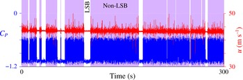
Figure 10 shows the time histories of the pressure coefficient measured at a port located at
 $\unicode[STIX]{x1D719}=90^{\circ }$
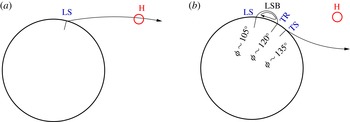
on spline A and the streamwise component of velocity acquired from a hot-wire probe in the near wake of the sphere, downstream of the pressure port. Both signals show highly correlated activity. The regions of low activity correspond to the LSB state. On the other hand, the non-LSB state is associated with a relatively early separation and large unsteadiness of the separated shear layer. Figure 11 shows a schematic of the flow and the ramification of the presence/absence of LSB on the hot-wire probe.
Time histories of
 $C_{P}$
at a port located at
 $\unicode[STIX]{x1D719}=90^{\circ }$
on spline A and streamwise component of velocity measured simultaneously at
 $Re=3.69\times 10^{5}$
. The hot-wire probe and pressure port lie on the same streamwise plane. Their relative location is indicated in figure 1.

Schematic of the flow past a sphere in the (a) non-LSB and (b) LSB states observed in subregime II of the critical regime. LS, TR and TS represent laminar separation, turbulent reattachment and turbulent separation, respectively. The approximate azimuthal locations for LS, TR and TS shown in panel (b) have been deduced from the pressure distribution shown in figure 9(b). Also shown is the location of hot-wire probe (H) for which the time history is shown in figure 10.

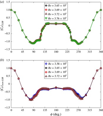
Angular distribution of the conditional time-averaged pressure coefficient for the (a) LSB and (b) non-LSB states for various
 $Re$
in the range
 $3.58\times 10^{5}\leqslant Re\leqslant 3.76\times 10^{5}$
.

Oil flow patterns at various
 $Re$
in various subregimes of the critical flow: (a) subregime I (
 $Re=3.40\times 10^{5}$
), (b) subregime II (
 $Re=3.70\times 10^{5}$
) and (c) subregime III (
 $Re=4.13\times 10^{5}$
). LS, TR and TS represent laminar separation, turbulent reattachment and turbulent separation, respectively.

(a) Probability density of
 $C_{D}$
at various
 $Re$
in the range
 $3.65\times 10^{5}<Re<3.75\times 10^{5}$
obtained from the time-series data. A threshold value of
 $C_{D}=0.12$
is used to estimate
 $I_{f}$
at each
 $Re$
. The value of
 $C_{D}=0.12$
is shown in panel (a) via the background colours. (b) Variation of the intermittency factor
 $I_{f}$
and
 $\overline{C}_{D}$
with
 $Re$
.

The time histories of
 $C_{P}$
at several
 $Re$
in subregime II of the critical regime are subjected to the same analysis as described earlier for
 $Re=3.69\times 10^{5}$
. At each
 $Re$
, the LSB and non-LSB states are identified from the base pressure and conditional time averaging is carried out. The average profiles are shown in figure 12. It is observed that
 $\langle C_{P}\rangle _{LSB}$
and
 $\langle C_{P}\rangle _{non\text{-}LSB}$
collapse, irrespective of the
 $Re$
in this regime. The
 $Re=3.58\times 10^{5}$
flow is associated with a non-LSB state only, while the
 $Re=3.76\times 10^{5}$
flow exhibits an LSB at all times. This confirms our hypothesis that the flow in this regime is a combination of the intermittent switch between the two states. It also shows that the intermittent nature of the LSB is restricted to subregime II of the critical regime. Oil flow visualization was carried out to explore the flow further. Figure 13 shows pictures of the oil flow visualization at various
 $Re$
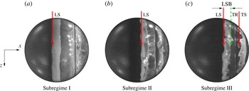
corresponding to subregimes I–III of the critical flow regime. To clearly bring out the phenomena on the surface of the sphere, the images were processed to remove the background colour. No changes have been made to the original images in the region lying within the sphere. Figure 13(a) shows the flow state in subregime I. The laminar boundary layer separates slightly upstream of the shoulder of the sphere (
 $\unicode[STIX]{x1D719}\approx 85^{\circ }$
). The oil upstream of the separation is pushed downstream, leaving a very clear signature of the line of separation. No reattachment of the separated flow is observed in this subregime. Figure 13(c) shows the flow in subregime III. In contrast to the flow in subregime I, the laminar separation occurs slightly downstream of the shoulder (
 $\unicode[STIX]{x1D719}\approx 105^{\circ }$
) and undergoes a turbulent reattachment at
 $\unicode[STIX]{x1D719}\approx 120^{\circ }$
. The turbulent boundary layer separates at
 $\unicode[STIX]{x1D719}\approx 135^{\circ }$
. As a result, an LSB that is bounded by laminar separation and turbulent reattachment is seen in figure 13(c) with very distinct boundaries. Figure 13(b) shows the flow in subregime II. Unlike in subregime III, the LSB in this subregime is intermittent. Consequently, the lines corresponding to turbulent reattachment and turbulent separation are not distinct, as in figure 13(c). However, the line corresponding to laminar separation is distinct, as expected. This image further supports our hypothesis that subregime II is associated with intermittent switching between LSB and non-LSB states. A similar phenomenon was demonstrated by Chopra & Mittal (Reference Chopra and Mittal2017) via a numerical study for flow past a circular cylinder. They utilized time averaging of the flow for one-tenth the time period of vortex shedding to show the intermittent nature of the LSB in the critical regime.
It is also interesting to note from figure 12 that
 $\langle C_{P}\rangle _{LSB}$
is relatively symmetric about
 $\unicode[STIX]{x1D719}=180^{\circ }$
in comparison to the
 $\langle C_{P}\rangle _{non\text{-}LSB}$
distribution. The suction in the non-LSB state is relatively large at
 $\unicode[STIX]{x1D719}=90^{\circ }$
as opposed to
 $\unicode[STIX]{x1D719}=270^{\circ }$
. This suggests that the formation of an LSB on the sphere is axisymmetric whereas the other activities related to the transition of the flow are not. In fact, figure 4 shows that the lateral forces on the sphere are non-zero in subregime II of the critical regime. This shows that the transition process is indeed sensitive to the manufacturing defects on the model. It is, therefore, quite remarkable that the formation of the LSB, which is one of the mechanisms in the entire transition process, appears to be axisymmetric despite the manufacturing defects.
3.5 Quantifying intermittency and its relation to the variation of
 $\overline{C}_{D}$
with
$Re$


The time histories of drag at various
 $Re$
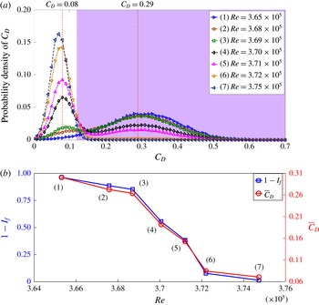
in subregime II of the critical regime are utilized to calculate the probability distribution function. These are shown in figure 14. All signals show either one or two peaks. These peaks exist at
 $C_{D}\approx 0.08$
and/or 0.29. A normal distribution with a single peak at
 $C_{D}\approx 0.29$
is observed for
 $Re=3.65\times 10^{5}$
. A bimodal distribution is observed at larger
 $Re$
. With increase in
 $Re$
, the probability of the state with
 $C_{D}\approx 0.08$
becomes larger while that of the state with
 $C_{D}\approx 0.29$
diminishes. In addition, as witnessed from the time-series data at
 $Re=3.70\times 10^{5}$
in figure 6(b), the standard deviation, i.e. the fluctuations, for the higher
 $C_{D}$
state are greater than those for the lower
 $C_{D}$
state. This is indicated by the broadness of the
 $C_{D}$
distribution about the higher
 $C_{D}$
peak in comparison to a relatively narrow distribution of
 $C_{D}$
about the lower peak. A gradual transfer of energy from the state with peak at
 $C_{D}\approx 0.29$
to the state with peak at
 $C_{D}\approx 0.08$
takes place with increase in
 $Re$
. For
 $Re=3.75\times 10^{5}$
and beyond, the distribution becomes Gaussian again with
 $\overline{C}_{D}\approx 0.08$
. We recall that the lower
 $\overline{C}_{D}$
corresponds to the LSB state while the higher
 $\overline{C}_{D}$
corresponds to the non-LSB state. As shown in figure 6 (for example at
 $Re=3.70\times 10^{5}$
), an intermittent switch between the LSB and non-LSB states occurs in subregime II of the critical regime. We define intermittency factor
 $I_{f}$
as the fraction of time spent by the flow in the LSB state. This is computed from figure 14(a) by choosing
 $C_{D}=0.12$
as a threshold value. A state for which
 $C_{D}$
is lower than this value is ascribed an LSB state. A value
 $I_{f}=1.0$
signifies a flow with an LSB at all times, while
 $I_{f}=0.0$
represents a flow that is completely devoid of an LSB. As an example,
 $I_{f}=0.5$
represents a flow where an LSB exists half the time. The threshold value of
 $C_{D}$
was chosen such that it leads to
 $I_{f}\approx 0.0$
at
 $Re=3.65\times 10^{5}$
and
 $I_{f}\approx 1.0$
at
 $Re=3.75\times 10^{5}$
. Figure 14(b) shows the variation of (
 $1-I_{f}$
) with
 $Re$
. Also shown in the same plot is
 $\overline{C}_{D}$
. We observe an excellent match in the variation of
 $\overline{C}_{D}$
and (
 $1-I_{f}$
) with
 $Re$
. This adds credence to our hypothesis that, during transition, there are two basic states – LSB and non-LSB. The time-averaged
 $C_{D}$
is a mean of these states weighted with the fraction of time spent therein.
The time histories of the back-pressure coefficient (
 $C_{P,b}$
) were also utilized to generate the probability density distribution at various
 $Re$
. This was then utilized to estimate the intermittency factor (
 $I_{f}$
). The variation of
 $I_{f}$
with
 $Re$
, from the pressure data, is similar to that shown in figure 14(b), except for one minor difference. The (
 $1-I_{f}$
) versus
 $Re$
curve from the pressure data shows an offset of
 $\unicode[STIX]{x0394}Re\approx 5300$
compared to that from the force measurement. This offset is attributed to the difference in the diameter of the sting used in the two measurements. In terms of the tunnel speed, the offset corresponds to
 $0.71~\text{m}~\text{s}^{-1}$
approximately. We note that this value of offset is quite insignificant compared to the range of speed (
 $45.33{-}58.67~\text{m}~\text{s}^{-1}$
) at which the drag crisis takes place for this model.
3.6 Laminar separation bubble and the three subregimes in the critical flow regime
The critical regime, as identified in figures 5 and 7, is extremely complex and has been further subdivided into three subregimes. Figure 15 shows the time variation of
 $C_{D}$
at one representative
 $Re$
in each of the three subregimes. The flow is devoid of an LSB in subregime I (figure 12). As seen in figure 15(a),
 $C_{D}$
undergoes relatively large fluctuations about a mean value. The time history of
 $C_{D}$
for
 $Re=3.70\times 10^{5}$
(subregime II), shown in figure 15(b), exhibits fluctuations about two mean states that alternate with each other. As discussed in earlier sections, the state with relatively lower mean drag is associated with an LSB while the relatively higher mean
 $C_{D}$
is related to a non-LSB state. The flow in subregime II is associated with intermittent appearance of an LSB. In subregime III (
 $3.75\times 10^{5}<Re<4.4\times 10^{5}$
), the LSB exists at all times. The drag is associated with relatively low mean and fluctuations. Compared to subregimes I and II, this subregime is relatively quiet with respect to flow phenomenon related to transition. Similar variation in
 $C_{D}$
is observed in the supercritical regime as well, as shown in figure 6(c).
The time variation of
 $C_{D}$
for (a)
 $Re=3.53\times 10^{5}$
, (b)
 $Re=3.70\times 10^{5}$
and (c)
 $Re=3.91\times 10^{5}$
corresponding to subregimes I, II and III of the critical regime, respectively.

Time variation of (a)
 $C_{D}$
, (b)
 $C_{Y}$
and (c)
 $C_{Z}$
at
 $Re=3.70\times 10^{5}$
(point highlighted in green in subregime II of figure 5
a). The colours in the background refer to the LSB and non-LSB states.

3.7 Axisymmetric nature of the laminar separation bubble and intermittency
We now explore the spatio-temporal nature of the LSB in the
 $Re$
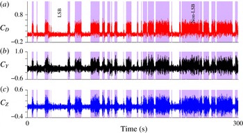
regime where it is intermittent (subregime II). We pose the following question: despite the possible manufacturing defects on the surface of the sphere, is the LSB really axisymmetric? To investigate this, we analyse the time series of the forces experienced by the sphere. Figure 16 shows the time histories of the drag and lateral forces at
 $Re=3.70\times 10^{5}$
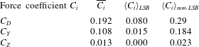
, which lies in subregime II of the critical regime. The LSB and non-LSB states are identified. As observed earlier, the fluctuations are relatively large in the non-LSB state. We note that all the time histories are highly correlated with respect to the intermittency of the LSB. The conditional time averaging for the LSB and non-LSB states is carried out for all the three force components. The results are compiled in table 1. Averages
 $\langle C_{D}\rangle _{LSB}$
and
 $\langle C_{D}\rangle _{non\text{-}LSB}$
have been discussed earlier. The conditional time average for the LSB state, due to flow reattachment and a narrow wake, is significantly lower than its non-LSB counterpart. Interestingly,
 $\langle C_{Y}\rangle _{LSB}$
and
 $\langle C_{Z}\rangle _{LSB}$
are close to zero, indicating the axisymmetric nature of the LSB. On the other hand,
 $\langle C_{Y}\rangle _{non\text{-}LSB}$
and
 $\langle C_{Z}\rangle _{non\text{-}LSB}$
are non-zero, suggesting a mean bias in the flow when it is in the non-LSB state. The analysis was repeated for all
 $Re$
in the critical regime. In all cases, the conditional time average of the lateral forces is close to zero for the LSB state. Once the LSB is completely formed, i.e. in subregime III of the critical regime and in the supercritical regime, the time-averaged lateral forces approach near-zero value (figure 4). Figure 17 shows a schematic of the flow phenomena on the surface of the sphere for the non-LSB and LSB states in subregime II of the critical regime.
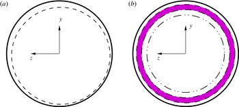
Schematic of the flow past a sphere in the (a) non-LSB and (b) LSB states in subregime II (
 $3.65\times 10^{5}<Re<3.75\times 10^{5}$
) of the critical regime. The shaded region indicates the approximate location where an LSB is observed. The dashed, dash-dotted and dash-double dotted lines indicate the approximate locations for laminar separation, turbulent reattachment and turbulent separation, respectively.

Conditional time-averaged force coefficients at
 $Re=3.70\times 10^{5}$
.

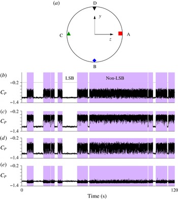
To further confirm that the LSB indeed forms and disappears at all polar locations simultaneously, we analyse the static pressure data acquired simultaneously at four locations on the shoulder of the sphere for
 $Re=3.69\times 10^{5}$
. The time histories of the
 $C_{P}$
at these four locations are shown in figure 18. The intermittent activity at all the locations is highly correlated, reconfirming the axisymmetric nature of the LSB. Interestingly,
 $\langle C_{P}\rangle _{LSB}$
for all the four probes is nearly the same (
 ${\approx}-1.1$
), which explains the nearly zero lateral force coefficients in the LSB state. On the other hand,
 $\langle C_{P}\rangle _{non\text{-}LSB}$
differs significantly for the four ports. For example,
 $C_{P}$
is
 $-1.2$
approximately, for the port on spline D, while it is
 $-0.6$
approximately, for that on spline B. This indicates a net positive
 $\langle C_{Y}\rangle _{non\text{-}LSB}$
, which is consistent with the force data in table 1. This observation reflects the robustness in the axisymmetric nature of the LSB.
(b–e) Time histories of the coefficient of pressure measured on the surface of a sphere at
 $\unicode[STIX]{x1D719}=90^{\circ }$
at the various ports shown in the schematic in panel (a): panels (b), (c), (d) and (e) show the data for ports lying along splines A, B, C and D, respectively.

4 Conclusion
The phenomenon of drag crisis for uniform flow past a smooth sphere is investigated experimentally via unsteady force and surface-pressure measurements and hot-wire anemometry. It is generally believed that the reduction in
 $\overline{C}_{D}$
with increase in
 $Re$
is mainly caused by an increase in the base pressure coefficient. However, surface-pressure measurements reveal that, in certain regimes, in addition to the increase in base pressure coefficient, the increase in suction in the region upstream of the sphere shoulder also plays an important role in the reduction of drag on a sphere with increase in
 $Re$
. The gradual decrease in
 $\overline{C}_{D}$
with increase in
 $Re$
in the high subcritical regime (
 $2.5\times 10^{5}<Re<3.4\times 10^{5}$
) is entirely due to the decrease in static pressure, upstream of the shoulder of the sphere. In the critical regime (
 $3.4\times 10^{5}<Re<4.4\times 10^{5}$
), the steep decrease in drag with increase in
 $Re$
is found to be a cumulative effect of the increase in base pressure coefficient and the peak suction upstream of the shoulder of the sphere. The location of peak suction gradually shifts downstream towards the sphere shoulder with increase in
 $Re$
. In the high-
 $Re$
part of the critical regime, as well as the supercritical regime, the peak suction is located very close to the shoulder of the sphere. Hence, the contribution of this increased suction to the decrease in drag gradually reduces with increase in
 $Re$
.
The critical flow regime is further divided into subregimes I–III based on the variation of coefficients of mean drag, base pressure and peak suction with
 $Re$
. This classification is useful in understanding the phenomenon of drag crisis. The space–time variation of the surface pressure is used to identify the LSB and its time evolution. The LSB exhibits different characteristics in the three subregimes. The dynamics of the LSB is found to correlate well with the variation of
 $\overline{C}_{D}$
with
 $Re$
in the critical regime. In subregime I (
 $3.4\times 10^{5}<Re<3.65\times 10^{5}$
), the flow is devoid of an LSB. It does not reattach once the boundary layer undergoes laminar separation. Subregime II (
 $3.65\times 10^{5}<Re<3.75\times 10^{5}$
) is associated with an intermittent LSB. The flow, during certain time intervals, reattaches as a turbulent boundary layer after the laminar separation. An LSB is observed during this period. However, there are also time intervals when the flow does not reattach and it is devoid of an LSB. The base pressure coefficient is utilized to identify the LSB and non-LSB states of the flow. The fraction of time during which an LSB exists increases with increase in
 $Re$
. The time instant when an LSB exists corresponds to a delayed flow separation and therefore to a relatively lower value of drag coefficient. On the contrary, the absence of an LSB is associated with relatively large value of drag coefficient. As a consequence, the time variation of drag coefficient is associated with bistable states in subregime II. The flow, at the end of subregime II, corresponds to an LSB state at all time instants. This state of flow continues throughout subregime III (
 $3.75\times 10^{5}<Re<4.4\times 10^{5}$
) where an LSB exists at all times.
The variation of
 $\overline{C}_{D}$
with
 $Re$
in subregime II is investigated in more detail. Since the drag is primarily determined by the pressure distribution, the evolution of the
 $\overline{C}_{P}$
–
 $\unicode[STIX]{x1D719}$
variation with
 $Re$
is also studied. At each
 $Re$
, the instantaneous flow is classified to be either in an LSB or non-LSB state based on the instantaneous value of the base pressure coefficient. Conditional time averaging of the force as well as surface-pressure coefficients, over the two states, is carried out to estimate
 $\langle ~\rangle _{LSB}$
and
 $\langle ~\rangle _{non\text{-}LSB}$
for the corresponding coefficients. It is found that, even though
 $\overline{C}_{P}(\unicode[STIX]{x1D719})$
shows significant variation with
 $Re$
, each of
 $\langle C_{P}(\unicode[STIX]{x1D719})\rangle _{LSB}$
and
 $\langle C_{P}(\unicode[STIX]{x1D719})\rangle _{non\text{-}LSB}$
show excellent collapse with respect to
 $Re$
. This shows that subregime II is primarily associated with only two states: LSB and non-LSB. The relative fraction of time interval for which the flow is associated with these states changes with
 $Re$
. To represent it quantitatively, an intermittency factor (
 $I_{f}$
) is estimated at each
 $Re$
:
 $I_{f}$
corresponds to the fraction of time spent in the LSB state, at each
 $Re$
. The value of
 $I_{f}$
is close to zero at the beginning of subregime II and increases to approximately one towards the higher end of subregime II. The variation of
 $\overline{C}_{D}$
with
 $Re$
is found to follow the relation:
 $$\begin{eqnarray}\overline{C}_{D}=I_{f}\langle C_{D}\rangle _{LSB}+(1-I_{f})\langle C_{D}\rangle _{non\text{-}LSB}.\end{eqnarray}$$
The values of
 $\langle C_{D}\rangle _{LSB}$
and
 $\langle C_{D}\rangle _{non\text{-}LSB}$
are estimated to be 0.08 and 0.29, respectively. This, to a large extent, explains the variation of
 $\overline{C}_{D}$
with
 $Re$
during the drag crisis. Such a phenomenology was also demonstrated recently by Chopra & Mittal (Reference Chopra and Mittal2017) for flow past a circular cylinder via a computational study. This points towards a possible universality in the
 $\overline{C}_{D}$
–
 $Re$
variation during drag crisis in bluff-body flows.
Another interesting aspect of the formation of an LSB explored in the study is regarding its spatial signature. In subregime II, where the LSB is intermittent, does it appear at all azimuthal locations simultaneously, or in patches? From simultaneous measurement of static pressure on the surface of the sphere at several polar locations, it is concluded that the LSB is axisymmetric. This is further substantiated by the conditional time averaging of the lateral force coefficients. Values of
 $\langle C_{Y}\rangle _{LSB}$
and
 $\langle C_{Z}\rangle _{LSB}$
are found to be close to zero throughout subregime II, even though
 $\overline{C}_{Y}$
and
 $\overline{C}_{Z}$
are non-zero. Values of
 $\langle C_{Y}\rangle _{non\text{-}LSB}$
and
 $\langle C_{Z}\rangle _{non\text{-}LSB}$
are, however, found to be non-zero, indicating a mean bias in the flow in the transitional regime. This bias might be due to the slight manufacturing defects in the model.
Acknowledgements
The authors would like to acknowledge Mr S. Saxena and Mr A. Pal of the National Wind Tunnel Facility, IIT Kanpur, for their help in conducting the experiments. The authors are also grateful to Mr G. Chopra for his enthusiastic participation in the discussion related to the statistical analysis of the experimental data.