




No CrossRef data available.
Human Capital and Growth in the Postbellum South: A Separate but Unequal Story
Published online by Cambridge University Press: 09 June 2004
Abstract
This article tests the importance of human capital in explaining convergence across the states from 1880 to 1950. Human capital matters to a state's income level and to its growth rate through technological diffusion. The South, whose overwhelmingly agricultural society relied more heavily on work experience than formal education, and whose racial discrimination in school resource allocation lowered human capital accumulation of both blacks and whites, presents a unique pattern. The South's low human capital levels following the Civil War and its active postbellum resistance to education reduced its speed of conditional convergence toward the rest of the nation.
Information
- Type
- ARTICLES
- Information
- Copyright
- © 2004 The Economic History Association
Both the convergence literature on regions within the United States and the literature on the evolution of the Southern economy have highlighted the need for an explanation of the slow convergence of Southern per capita income to that of the rest of the United States after the Civil War.
Kris Mitchener and Ian McLean identify the West and the South as key regions in explaining the convergence pattern of the United States from 1880 to 1980.1
Mitchener and McLean, “U.S. Regional Growth.”
Ibid., p. 1021.
Of the observed convergence between Southern and Northern average service income between 1880 and 1950, Caselli and Coleman (“U.S. Structural Transformation”) show that up to 81 percent is attributable to structural transformation. For the 1940 to 1990 period, structural transformation is empirically less important than in the earlier period, but still accounts for approximately 57 percent of the measured convergence between the two regions. The remainder is explained by within-sector North-South wage convergence. Caselli and Coleman therefore focus on modeling the Southern structural transformation caused by labor movement out of agriculture and the subsequent rise in agricultural wages relative to manufacturing wages. This insightful model is able, in positive terms, to explain the role of structural transformation in the observed pattern of service income convergence. The key assumption generating this structural transformation is a long-run decline in the relative costs of acquiring nonagricultural skills in both regions.
Mitchener and McLean, “U.S. Regional Growth,” p. 1030.
Mitchener and McLean, “U.S. Regional Growth”; Williamson, “Growth”; and Williamson and Lindert, American Inequality.
Instead, one must explain the relatively low productivity in the South in the postbellum period as well as gradual convergence in productivity to that of the rest of the nation to explain Southern convergence.6
Margo, “North-South Wage Gap.”
A wide range of factors have been proposed to explain the South's relative stagnation in the postbellum period. Wright (“Cotton Competition”) focuses on poor world demand for cotton, Ransom and Sutch (One Kind) on the reduced agricultural labor supply, and Carlton and Coclanis (“Capital Mobilization”) on the lack of adequate capital for industrialization.
Wright, Old South.
The regions are defined as follows: North Atlantic: Connecticut, Maine, Massachusetts, New Hampshire, New Jersey, New York, Pennsylvania, Rhode Island, and Vermont; North Central: Illinois, Indiana, Iowa, Kansas, Michigan, Minnesota, Missouri, Nebraska, North Dakota, Ohio, South Dakota, and Wisconsin; South Atlantic: Delaware, Florida, Georgia, Maryland, North Carolina, South Carolina, Virginia, and West Virginia; South Central: Alabama, Arkansas, Kentucky, Louisiana, Mississippi, Oklahoma, Tennessee, and Texas; and Western: Arizona, California, Colorado, Idaho, Montana, Nevada, New Mexico, Oregon, Utah, Washington, and Wyoming.

FIGURE 1 EDUCATION-BASED HUMAN CAPITAL
Given the strong relationship present in Figure 1, I test the contribution of human capital to both income levels and growth in 48 states of the United States from 1880 to 1950. Controlling for possible reverse causality, I find that along with physical capital, a state's human capital stock significantly contributes to both the level and growth of its income. Moreover, I am able to consider the theory that racial discrimination in Southern education was a primary contributor to the low levels of human capital, not only for Southern blacks, but for Southern whites as well.
GROWTH THEORY
Robert Solow's neoclassical growth model predicts convergence in income per capita among countries conditional on identical production functions, savings rates, and labor force growth rates, without requiring factor mobility.10
Solow, “Contribution.”
Barro and Sala-i-Martin, “Convergence across States” and “Convergence.”
The answer to this question may lie in human capital differences between the states. In human capital models of endogenous growth, growth is driven by the accumulation of human capital, broadly defined as an individual's skill level accumulated through formal education or through on the job learning-by-doing.12
Uzawa, “Optimum Technical Change”; Lucas, “On the Mechanics”; and Romer, “Increasing Returns” and “Endogenous Technical Change.”
Because human capital accumulation is the driving force in these models, absolute convergence will not necessarily occur between countries with different initial levels of human and physical capital, unless factor mobility forces convergence. Between 1880 and 1900, Southern income per capita grew at about the national rate. It did not greatly converge with the rest of the nation until after the turn of the century, when labor mobility increased and educational and skill differentials began narrowing.13
Wright, Old South.
Wright, ibid.; and Rosenbloom, “One Market” and “Was There.”
HISTORICAL SETTING
Four factors contributed to the South's emergence at the turn of the century as a low-wage, low-skill region specializing in labor-intensive industries. They include the South's plantation legacy, its active resistance to educating its workforce, both black and white, the relative isolation of its labor market, and “backwash” effects of being a latecomer to industrialization.
The legacy of slavery and reliance on a plantation economy left the South without a significant industrial structure or labor force capable of quickly adapting to industrialization after the Civil War. David Weiman argues that slavery and labor-intensive plantation technology in the South resulted in both reduced investment in physical capital and a reduced labor supply for prospective Southern manufacturing industries prior to the Civil War.15
Weiman, “Staple Crops.”
Wright, Old South; and Beatty, “Lowells.”
The plantation legacy also left the South with very little human capital relative to the rest of the nation immediately after the Civil War. The reasons for this are quite straightforward. By 1835, there existed a uniform legal proscription across the South against the formal education of slaves as a result of slave insurrections earlier in the nineteenth century. Consequently, 95 percent of the black Southern population was completely illiterate at the beginning of the Civil War. Furthermore, the lagged effect of older generations tended to slow educational improvements for younger generations.17
Smith, “Race”; and Margo, Race.
Using data from the 1910 Census, Margo (Race and Schooling) finds that school attendance rates rose 4.2 percent with a 10-percent reduction in adult illiteracy.

FIGURE 2 SOUTHERN LITERACY (percentage of the population over the age of 10)
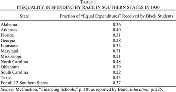
Moreover, although state funds were allocated on a per pupil basis independently of race, within the segregated schooling system (and aided by disfranchisement after 1877), states diverted funds at the local district level from black schools to white schools.19
Bond, Education; Margo, “Race, Educational Attainment” and Race; and Gerber, Southern White Schooling.
Gerber, Southern White Schooling, pp. 9, 13.
Bond, Education.

Black schools in the South were marked by lower teacher salaries, higher student to teacher ratios, shorter terms, and lower educational levels of teachers.22
For example, in 1911 in Georgia, black teachers earned less than half of what white teachers earned, black schools generally had twenty more students per class than white schools, the school term was three to four weeks shorter and only 16 percent of black teachers had at least two years of postsecondary education, compared to 35 percent of white teachers (Donohue, Heckman and Todd, “Schooling,” p. 229).
Donohue, Heckman and Todd, “Schooling.”
Card and Krueger, “School Quality.”
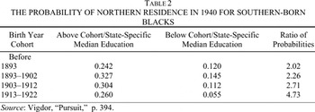
In the prewar era, there is ample evidence of selective migration of more educated blacks out of the South.25
Margo, “Schooling” and Race; and Vigdor, “Pursuit.”
Vigdor, ibid.

Using U.S. Census microdata on blacks, Jacob Vigdor demonstrates positive intergenerational effects between the education level of parents who migrated between 1940 and 1970 and educational attainment of their children in 1970 and 1990.27
Vigdor, ibid.
Smith, “Race and Human Capital”; and Margo, Race.
The large fraction of the labor force composed of blacks (about 46 and 58 percent of the South Central and South Atlantic populations respectively in 1890), combined with severe racial discrimination in schooling and selective migration of more educated blacks out of the South, were sufficient to lower Southern human capital levels relative to the rest of the nation.29
Abstract of the Twelfth Census, 1900, (1904), p. 41.
Smith, “Race and Human Capital.”

FIGURE 3 MEAN SCHOOLING LEVELS IN MONTHS
Even aside from issues of racial discrimination, the South had a historical legacy of low education norms. James Gerber points to the lack of property tax use for public education to explain the limited resources for public education in the South prior to Reconstruction.31
Gerber, Southern White Schooling.
Ibid., pp. 5–8.
Using 1940 U.S. census data, Gerber finds that between 20 and 25 percent of lower individual incomes of all Southern men were attributable to lower educational attainment.33
Ibid.
Ibid, pp. 30, 33–34.
Still, it could be argued that the widespread discrimination against blacks in the South may have resulted in depressed support for public education in general because of the inability of lower-class whites to join political forces with blacks in support for public education. Gerber explains:
In the case of school finance, the gulf between black and white Southerners was exacerbated by the racist propaganda that attempted to convince lower-class whites that state school revenues derived from white citizens were going to black schools. Given the inadequacy of white schools in many areas, this argument raised racial tensions and prevented, or at least hindered, a unified front of poor whites and blacks from demanding better schools. Those whites who benefited saw no need to support campaigns for higher taxes for schools: they could always raid the funds intended for black schooling when they desired more revenue…. Even though this type of discrimination was aimed ostensibly at the black population, it may have affected lower-class whites as well, much in the same manner that disfranchisement removed the vote from significant numbers of poor and illiterate whites.35
Ibid, p. 99.
Along these lines, Gerber finds that, for Southern states, the higher the percentage of blacks in the state population, the higher the level of white schooling inequality.36
This was not the case for non-Southern states. Gerber, ibid., pp. 115, 126.
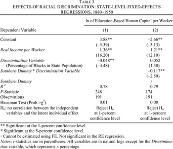
Using the education-based measure of human capital per worker, it is possible to indirectly consider the hypothesis that, within the South, higher percentages of blacks in the population would have led to easier redistribution of school resources towards white pupils, and therefore to lower incentives for politicians to argue in favor of greater overall resource allocation towards public education. Because the education-based measure of human capital is based on school expenditures, it lends itself well to this question. I therefore run a state-level panel regression for 1880, 1900, 1920, and 1950 of education-based human capital per worker on income levels and the percentage of the state population that was black.37
Data on the percentage of state populations that are black come from Gibson and Jung, “Historical Census Statistics.”
This admittedly simple regression is intended to see if there is support for the notion that racial discrimination contributed significantly to lower educational standards for the average Southerner (rather than just for the average black Southerner). Because state income is clearly a primary determinant in resources potentially available for education, it is included to control for the fact that Southern states were also lower income states. The results from this simple regression are intriguing. Column 1 of Table 3 presents the results using fixed effects (FE) estimation for all states of the United States.38
FE estimation treats unobservable latent individual effects as fixed and focuses on deviations of states over time from their individual means. This is identical to having a dummy for each state in the regression. Further descriptions of this estimation technique are provided in a later section.
When the regression is run only for the South, the discrimination variable is statistically significant and negative, whereas when run only for non-Southern states, the discrimination variable is not significant.

Finally, there was strong opposition from both industrial employers and planters to educating the common laborer, whether black or white, for fear that educated workers would leave the South.40
Wright, Old South.
Evidence, such as the slowness with which the South adopted mechanization in cotton, suggests that the Southern plantation system was relatively traditional and not modernizing relative to the rest of the nation, even compared to other agricultural regions (Gerber, Southern White Schooling).
Gerber, Southern White Schooling, pp. 91–93.
Although school expenditures always rely upon the contemporaneous economic situation, this negative attitude towards education driven by employer pressures and racial discrimination was largely responsible for the fall in real Southern school expenditures per pupil in the post-bellum period (Figure 4). No concerted effort was made to change the quality of the Southern educational system at least until the turn of the century. There was significant improvement in the percentage of school-aged children in the South who attended school.43
U.S. Bureau of Education, Report, 1893, p. 36, and 1911, p. 694.
Wright (Old South) argues that these wage gaps for unskilled labor were not merely the result of racial discrimination. Although racial discrimination occurred, and racial wage gaps existed, the North-South wage gap for unskilled labor was significantly larger than the racial gap.

FIGURE 4 REAL ANNUAL SCHOOL EXPENDITURE PER PUPIL (1967 dollars)
A final consideration for the South during this period is its position as a periphery region relative to the core of the North. Specifically, the appearance of a more national product market during this time period offered new opportunities, but also placed the South in a latecomer position relative to the North and even the West. One can view the Southern experience of industrialization as suffering from both Albert Hirschman's “polarization” and Gunnar Myrdal's “backwash” effects, whereby in early periods of development market forces accentuate initial disparities across regions.45
Hirschman, Strategy; and Myrdal, Economic Theory.
Williamson, “Regional Inequality”; Carlton, “Revolution”; and Carlton and Coclanis, “Capital Mobilization.”
Williamson, “Regional Inequality.”
Ibid., pp. 5–9.
Evidence of these effects was present in the South, as demonstrated by selective migration patterns for blacks that later become less selective, and selective choices for industrialization. David Carlton describes the Southern choices for industrialization as limited by the lack of entrepreneurial expertise and labor skills, leading the region “…to compensate by developing or attracting industries at advanced stages in the product cycle, industries in which skills have been largely ‘built in’ to their basic technology and structure.”49
Carlton, “Revolution,” p. 473.
This also implies that capital-goods industries will locate in areas with a sufficient stock of skilled labor and demand for specialized products. In turn, once situated, these industries will attract and expand the local mass of skilled workers.50
Carlton and Coclanis, “Capital Mobilization.”
Ibid.
Carlton and Coclanis, “Uninventive South,” pp. 321–22.
In line with the theories of polarization and backwash effects, Sukkoo Kim empirically demonstrates the importance of factor proportions to the location of industries in the United States.53
Kim, “Expansion.”
Kim, “Economic Integration.”
Ibid., pp. 660–61.
Kim notes that the primary cause of income divergence in the U.S. between 1840 and 1900 was the relative decline in Southern per capita income “…caused by the region's growing unfavorable industry-mix and lower wages relative to other regions.” He calculates that Southern income per capita would have risen by as much as 20 percent had its industrial structure converged towards that of the national average (Kim, ibid., p. 672).
Both issues—low investment in education, primarily for blacks but also for whites, and core and periphery—rely on increased labor mobility for final resolution of the inequalities across regions. Hence, greater levels of labor movement between the South and the rest of the nation were necessarily part of the final conditional convergence of the South to national norms.
A key part of the migration story relies on the migration pattern of Southern blacks. Immediately after emancipation blacks began to shift locations, but the movement was generally local (i.e., within the county of origin or between contiguous counties).57
To the extent that there was longer distance migration of blacks it tended to occur in a westerly direction within the South (Higgs, Competition, pp. 24, 26).
In both 1860 and 1910 approximately nine-tenths of the black population lived in the South. This held despite positive net migration of blacks to the North because of higher fertility and lower mortality in the South than in the North (Higgs, Competition, p. 28).
Only after the drastic reduction of foreign immigration to the United States beginning around 1920 and peaking in the late 1920s and early 1930s did employment opportunities in the North increase for blacks, leading to greater (nonselective) black migration northward.59
On immigration, see Lebergott, Manpower, pp. 29, 163; and Easterlin, Population, pp. 187–88. On black migration, see Higgs, Competition, p. 26.
Colberg, Human Capital.
In summary, the plantation legacy, combined with low educational standards, labor market isolation, and periphery effects, left the South to industrialize almost completely without the aid of an indigenous technical community. Consequently, Southern firms were dependent upon Northern technology, but lacked a sufficiently educated labor force to aid in the adoption or possible adaptation of Northern technology to Southern needs.61
For striking examples of this in the textile industry see Beatty, “Lowells.”
As suggested by Richard Nelson and Edmund Phelps, human capital increases the rate at which existing technology can be applied for practical uses.62
Nelson and Phelps, “Investment.”
Wright, Old South.
GROWTH ACCOUNTING
The regressions undertaken here draw from growth accounting. I first consider level regressions similar to those of Gregory Mankiw, David Romer, and David Weil and then comparable growth regressions along the lines of Jess Benhabib and Mark Spiegel's. 64
Mankiw, Romer, and Weil, “Contribution”; and Benhabib and Spiegel, “Role.”
Growth accounting regressions are generally based on the following Cobb Douglas production function:

where Y is real state income, A is the technology level, K is the real capital stock, H is the human capital stock, and L is the number of employed workers in the state. In per worker terms, equation 1 becomes

where all lower case letters are the original variables expressed in per worker terms. In natural logarithmic form, for each state, i, equation 2 becomes

This equation likely neglects certain unobservable state specific effects. Hence, the regressions to follow test equation 3 with a one-factor error term, μit, where μit=αi+εit, i=1…48, and t=1…4. Following Jerry Hausman and William Taylor, αi represents an unobservable latent individual state effect.
65Hausman and Taylor, “Panel Data.”
Estimation by Ordinary Least Squares (OLS) assumes no latent individual effects. Hence, OLS will be inefficient if such effects are present. Fixed effects (FE) estimation treats latent individual effects as fixed, focusing on deviations of states over time from their individual means. FE estimation also yields inefficient estimates. However, by treating the αι as fixed, the FE estimates will be unbiased and consistent regardless of whether or not there is correlation between the individual effects and the explanatory variables. Random effects (RE) estimation allows for random latent individual effects and represents a weighted average of both cross-sectional and within-group variance. In the absence of correlation between the αι and the explanatory variables, RE estimation will be BLUE. If however, such correlation is present, then its results will not be consistent. Because such correlation affects FE and RE estimators differently, differences in the estimated coefficients suggest possible correlation (Hausman, “Specification Tests”). Accordingly, rejection of the null hypothesis of no correlation suggests that the FE estimates are the only consistent estimates.
In addition to the basic relationship in equation 3, growth regressions are run on equation 3 using natural log differences. These growth regressions are further supplemented following a methodology similar to that of Benhabib and Spiegel.
67Benhabib and Spiegel, “Role.”
Nelson and Phelps, “Investment.”

where c reflects exogenous technological progress, g(hi) reflects endogenous technological process within the state, and m[hi(ymax−yi)/yi] embodies the notion of technological diffusion or catch-up to the most advanced state. Both g([bull ]) and m([bull ]), are nondecreasing functions of hi. We can regroup the hi terms and write equation 4 as

The catch-up term in equation 4′ should depend on relative technology levels, rather than relative income levels. However, Benhabib and Spiegel use y as a proxy for A in the catch-up term, as the technology level is inherently difficult to measure. The technology level is even more difficult to quantify for individual states from 1880 to 1950. I therefore also use y as a proxy for A in the diffusion term. Applying equation 4′, the growth accounting specification with catch-up becomes

where I use natural logs for the level of hi and the catch-up term.
DATA
The model is tested using panel data from 48 states in 1880, 1900, 1920, and 1950. These are the only years for which both capital stock and income data are available by state. Data on each state's capital stock (except for 1950), workforce, and personal income for these years are from estimates by various authors in Population Redistribution and Economic Growth: United States, 1870–1950, edited by Simon Kuznets and Dorothy Swaine Thomas. I create a 1950 capital stock estimate to supplement the existing series using data from various issues of the Annual Survey of Manufactures, and from works by Thomas Romans and John Kendrick.69
Romans, Capital Exports; and Kendrick, Productivity Trends.
I also create two estimates for the human capital stock in each state from 1880 to 1950. The first reflects human capital accumulated through formal education, and the second reflects human capital accumulated through work experience. I first consider the two types of human capital separately and then interact the two measures to create a more comprehensive human capital term.
Formal education can be measured in terms of quantity of education (for example, years of education) or in terms of quality of education (i.e., school expenditures, teacher salaries, teacher education, and teacher-pupil ratios). However, Margo argues that yearly school attainment data before 1910 are biased because of the interpretation that a year of schooling in an ungraded Southern school, with shorter school terms and less trained teachers, was measured as being equal to one grade level in the rest of the nation.70
Margo, “Race and Human Capital.”
Rizzuto and Wachtel, “Further Evidence,” p. 241.
When examining the effect of school quality on individual earnings, two issues arise. The first is whether school inputs, as a measure of school quality, actually have any effect on earnings. Julian Betts provides a comprehensive survey of the relevant empirical studies and shows that studies focusing on individuals educated after 1960 tend to find little or no role for school inputs in explaining student earnings.72
Betts, “Is There a Link.”
These are simple cross-study averages of the percentage of the reported regressions in each study where the stated school input is significant at the 5-percent confidence level. Betts, “Is There a Link,” table 6-1, pp. 144–45.
The school expenditure data come from annual reports from 1870 to 1915 and from biennial reports until the 1950s by the U.S. Commissioner of Education. A detailed description of the perpetual inventory method is given in the appendix.
Lee, “Migration Estimates.”
For the experience-based human capital measure, I use data on the age profile of the workforce for each state from Ann Miller and Carol Brainerd's labor force estimates, along with years of schooling and literacy data for annual birth cohorts by state of residency created from the 1920, 1940, and 1960 U.S. Censuses to create a proxy for the average work experience of a worker in each state.76
Miller and Brainerd, “Labor Force Estimates,” pp. 362–517, presented in Kuznets and Thomas, Population Redistribution. Ruggles, Sobek et. al., IPUMS.
All data (except for the experience-based human capital measure) are first converted to real terms (1967 dollars) using a national consumer price index (CPI).77
U.S. Department of Commerce, Historical Statistics, pp. 210–11.
Mitchener and McLean, “U.S. Regional Growth.” I thank Kris Mitchener and Ian McLean for providing me with their data.
In interpreting the results that follow it is also important to stress the fact that the data used are estimates constructed from survey or census data from 1870 to 1950. Given the dates of the surveys, there is likely a great deal of measurement error in the raw data, as well as possible biases due to the procedures used to create time-consistent series.
RESULTS
Level Regressions
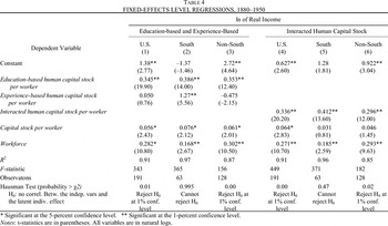
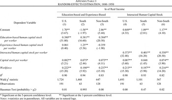
In Table 4, fixed effects (FE) estimation results are presented for equation 3.79
OLS regressions with robust standard errors were also undertaken for the four time periods separately. The results are consistent with the panel regression results of Table 2 and suggest a fair amount of stability over time.
Hausman, “Specification Tests.”


The first three columns of Table 4 present results from FE estimation of equation 3 respectively for the United States, the South, and the Non-South, in 1880, 1900, 1920, and 1950 jointly, when the two human capital measures are considered separately. All variables are in natural logs. The results are good. In the three level regressions, all of the explanatory variables have the expected signs and are statistically significant, with the exception of the experience-based human capital measure, which is not significant for the United States and is negative for non-Southern states. For the United States as a whole, the coefficient estimates for education based human capital and physical capital are 0.35 and 0.06 respectively. The coefficient estimate for education-based human capital is statistically significant in all three regressions and yields similar estimates for the two regions and the nation as a whole. On the other hand, findings for the experience-based human capital measure vary greatly across regions. Only in the South does this proxy for on-the-job training show up positively and significantly. Moreover, for the Southern states, the coefficient estimate for experience based human capital is 1.27, relative to the 0.39 coefficient on education-based human capital. This result is in line with the observation that a majority of the workforce in Southern agricultural society had little to no formal education, and hence output relied heavily on learning gained through work experience. The result further underscores a potential inflexibility within Southern states in shifting to new types of industry, because on-the-job training is less likely to be useful for a worker shifting from an agricultural job to an job in industry than is learning based on formal education that will serve the worker in all work settings.
The effects of migration are captured within the education-based human capital estimate, which is adjusted for migration. In order to directly consider the effects of migration, the same regression was run including the education-based human capital measure without the migration adjustment and the natural log difference in this measure when migration is taken into account. Both the raw human capital term and the migration adjustment are statistically significant. The elasticity of real income with respect to the raw education based human capital stock is 0.17 and with respect to the migration adjustment is 0.26. This suggests that migration, or more specifically migration of the human capital embodied in individuals, played a very important role in determining per worker income levels across states. Moreover, because the migration adjustment used here assigns the average education-based human capital stock to an individual based on his or her state of birth, the measured effect of migration is likely underestimated. Given the previously discussed evidence of educational selectivity of individuals choosing to migrate, the true effects of migration are likely larger than those documented here.
Columns 4 through 6 of Table 4 present the same regression for the United States, the South, and the Non-South using an interacted education and experience human capital stock measure.81
To control for possible technological progress, the national regression was run first using a time trend and then using time dummies. The time trend is not significant and leaves the remainder of the regression results basically unchanged. Only the time dummy for 1950 is significant (and positive) in the FE regression. Again the results presented in Table 4 remain.
There is, of course, an issue of possible reverse causality between income and investment in human capital, which could be driving the results. To control for the possibility of dual directions of causation, three different regressions are considered. First, a panel instrumental variable regression was run using lagged human capital levels as an instrument for the human capital term. The results from this regression follow those of column 4, Table 4 extremely closely. The only differences are a slightly higher R2(0.93), a larger coefficient (0.44) on the interacted human capital term, and fewer observations (because the use of a lagged variable as an instrument prevents the use of observations from 1880). Second, the regression was again run for the 1900 to 1950 time periods, including 1880 state income per worker as an explanatory variable. Third, in a slightly stronger test, lagged income levels are included as independent variables. If high investment in human capital (through school expenditures) is solely the consequence of high state wealth, then the human capital stock coefficient should become insignificant once initial income, or lagged income, is included. In the separate regressions, both initial 1880 income and lagged income are statistically significant and positive, with coefficient estimates of 0.07 and 0.2 respectively.82
The RE estimate for 1880 income is presented because FE estimation cannot estimate a constant variable.
A final issue to consider is that of omitted variables. It is possible that there are omitted variables that may be correlated with human and physical capital stock variables.83
For example, a state's policy environment is likely to be correlated with its investment in human and physical capital, leading to a positive bias on the human and physical capital coefficients if ignored.
Growth Regressions
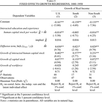
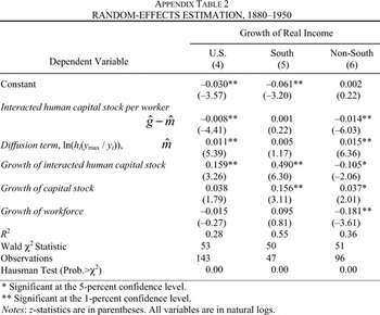
Table 5 presents growth regression results for the United States, the South, and the Non-South from 1880 to 1950, following the Benhabib and Spiegel catch-up specification of equation 5. It is worth highlighting the interpretation of the coefficient estimates on hi and the catch-up term. Specifically, g reflects possible endogenous technological progress, while m reflects the catch-up component due to technological diffusion. If one looks at national patent data, we see that innovative activity is concentrated in only a handful of countries. This pattern is likely to also hold within a country. That is, if most endogenous technological progress is occurring in a few lead states and then diffusing to the rest of the nation, one should expect that m will be greater than g. Note also that the concept of conditional convergence is embodied in the notion of technological diffusion: conditional convergence, if present, is occurring through technological diffusion and will be evidenced by a positive and statistically significant estimate for m. Moreover, it is important that the estimate for g be less than that for m, because if g were greater than m throughout the United States, endogenous technological progress would exceed diffusion, implying divergence in technology and income levels across states. This implies that the coefficient estimate (g−m) on ln hi should be negative.
The results are presented in Table 5. Both the growth of physical and interacted education and experience human capital contribute to income growth per worker, with statistically significant coefficients of 0.08 and 0.4 respectively.84
The finding that human capital growth matters to income growth demonstrates an important role for human capital as an input into production itself, which Benhabib and Spiegel (“Role”) do not find in their 1965–1980 cross-sectional country regressions.
Capital Stock
The lack of available capital is often cited as having limited the speed of Southern industrialization.85
Carlton and Coclanis, “Capital Mobilization”; and Wright, Old South.
Using a cross-country regression for 1965, Benhabib and Spiegel (“Role”) find that the human capital level of a nation positively affects its physical capital accumulation.
Labor is positive but marginally insignificant and the current capital stock enters negatively and significantly as expected with diminishing returns to capital.
CONCLUSION
This article finds two crucial roles for human capital in explaining the growth and convergence pattern of states after the Civil War. In particular, human capital levels are shown to matter not only to a state's income level, but also to its growth rate, both directly as an input into production and indirectly through technological diffusion.
Still, there is a unique pattern in the South, whose overwhelmingly agricultural society relied more heavily on work experience than formal education, whose racial discrimination in school resource allocation played a crucial role in lowering human capital accumulation of both blacks and whites, and whose investment in physical capital is found to have depended on human capital accumulated through formal education rather than through work experience.
Not only is this last aspect of the Southern experience consistent with the notion that experience-based human capital may be more job specific and therefore less useful than education-based human capital when considering switching to new industries, but it also provides support to the argument that the South's lack of emphasis on formal education slowed both investment and growth.
In levels, the elasticity of state income per worker in terms of interacted human capital per worker is found to be approximately 0.34. In growth terms, the elasticity of per worker income growth with respect to growth of human capital is 0.4 and with respect to the role of human capital in technological diffusion it is 0.03 times the percentage income gap relative to the richest state.
The fundamental question is this: why did the South not industrialize rapidly after the abolition of slavery? The lack of available capital is often cited as having limited the speed of Southern industrialization.88
Carlton and Coclanis, “Capital Mobilization”; and Wright, Old South.
After the Civil War, the South did not catch up with the educational standards of the rest of the nation. So long as pronounced educational and skill differences existed between the South and the rest of the United States, real Southern per capita income did not quickly converge towards the national norm. This was due to both level (productivity) effects and growth (technological diffusion) effects. Had the South been able to more quickly increase its human capital levels, particularly through formal education, it would have benefited both from a greater speed of convergence with the rest of the nation, as well as from a greater absolute convergence in income levels with the rest of the nation.
Appendix: Data
Education Based Human Capital
Annual estimates for the stock of human capital per worker generated from formal education in each state from 1870 to 1950 are based on total school expenditures data (from annual reports from 1870 to 1915 and from biennial reports until the 1950s by the U.S. Commissioner of Education) and on migration data from Lee.
89Lee, “Migration Estimates.” Data from Dakota is used for North and South Dakota in 1880 because this territory had not yet been separated into two states at that date. Oklahoma is missing all 1880 data.
, are constructed from real annual school expenditure data, St, as a measure of investment in education, using the perpetual inventory model:

where δ is a depreciation (or obsolescence) rate reflecting the fact that human capital disappears as people forget or die. A depreciation rate of 10 percent is used because this implies that only 1 percent of initial human capital is left after 44 years.
90Other rates such as 5 percent and 20 percent are also tested yielding generally similar regression results.

where g is the average annual growth rate (in ln differences) of real school expenditures from 1870 to 1950 and S* is a weighted estimate of the steady-state value of investment based on the following formula:

The raw human capital stock estimates are then adjusted for interstate migration using data derived by Lee.
91Lee, “Migration Estimates.”
Experience Based Human Capital:
Estimates of the average work experience of laborers in each state are derived by first estimating the average work experience of people born within a specific birth cohort by state of residence using data on average years of schooling from the 1940 and 1960 U.S. Censuses.92
All of the census data come from the Integrated Public Use Microdata Series: Version 2.0 (Ruggles, Sobek, et al., 1997: http://www.ipums.org).
This panel regression with 3,233 observations yields a coefficient estimate of 3.98 for the literacy index (which ranges from 1 (completely illiterate) to 4 (completely literate)) with an R2 of 0.36 and an Wald statistic of 964.
Average annual cohort experience in year x=age of worker in year x−average years of schooling for that birth cohort−6
Miller and Brainerd, “Labor Force Estimates,” pp. 372–80, table 2.4.
The need for some predicted values for years of schooling is a strong drawback to this experience measure. Because the earliest birth cohorts rely more heavily on predicted values (i.e., generally prior to 1849), the importance of the predicted values is significant for 1880 estimates but diminishes quickly with time. For example, in the 1880 estimate of average work experience, approximately 26 percent of the U.S. labor force was born before 1835 (71 percent before 1855).95
These two cutoff dates are reported here since these are the two end years for relevant birth cohort groupings reported in the age profile labor data.
Capital Stocks
Easterlin provides estimates for the capital stock in manufacturing for each state in 1880, 1900, and 1920. These estimates are based on census reports on the gross assets of manufacturing establishments, including land, buildings, machinery, and cash, but excluding rented capital.
96A detailed explanation of the construction of this series is available in Kuznets and Thomas, Population Redistribution, pp. 675–78.

where g is the average annual growth rate (in ln differences, using the three year averages to smooth out the endpoints) of real investment in new plant and equipment in the manufacturing sector from 1951 to 1976 based on data from the Annual Survey of Manufactures (ASM), various issues, and δ is a depreciation rate of 8 percent (chosen to match Easterlin's assumed depreciation rate). I1950 should ideally be investment data in 1950. However, no data for investment in 1950 are available by state. Hence I consider three proxies for this measure. The first is Romans's estimates of investment in new plant and equipment by state in 1953, which uses ASM data appropriately adjusted to match aggregate U.S. manufacturing data from various issues of the Survey of Current Business.
97Romans, Capital Exports.
Finally, estimates for the capital stock in manufacturing in each state in 1880, 1900, 1920, and 1950 are proportionately scaled up to match the time series behavior of the aggregate U.S. physical capital stock using data on the real capital stock for the U.S. private nonfarm nonresidential sector from John Kendrick.98
Kendrick, Productivity Trends.
Personal Income
Personal income data come from estimates by Richard Easterlin in Kuznets and Thomas.99
Easterlin, “Regional Growth.”
Kuznets and Thomas, Population Redistribution, pp. 703–27.
Labor Force
Ann Miller and Carol Brainerd estimate labor force data in Kuznets and Thomas using decennial censuses of the population for the period 1870–1950.101
Miller and Brainerd, “Title,” pp. 364–411.
I thank Erica Groshen, Vassilis Hajivassiliou, James Harrigan, Sebnem Kalemli-Ozcan, Thomas Meyer, Carol Osler, Gabriel Perez-Quiros, Xavier Sala-i-Martin, David Weiman, Kirk White, Jeffrey Willamson, Eric van Wincoop, Gavin Wright, Kei-Mu Yi, and two anonymous referees for valuable comments. Sairah Burki, Joseph Davis III, and Jenessa Gunther provided valuable research assistance. I remain responsible for any errors.
References
Barro Robert, and
Xavier Sala-i-Martin.
1991
“Convergence across States and Regions.”
Brookings Papers on Economic Activity,
no. 1:
107–
82.Google Scholar
Barro Robert, and
Xavier Sala-i-Martin.
1992
“Convergence.”
Journal of Political Economy
100,
no. 2:
223–
51.Google Scholar
Beatty Bess.
1987
“Lowells of the South: Northern Influences on the Nineteenth-Century North Carolina Textile Industry.”
Journal of Southern History
53,
no. 1:
37–
62.Google Scholar
Benhabib Jess, and
Mark Spiegel.
1994
“The Role of Human Capital in Economic Development: Evidence from Aggregate Cross-Country Data.”
Journal of Monetary Economics
34,
no. 2:
143–
73.Google Scholar
Betts Julian.
1996.
“Is There a Link between School Inputs and Earnings? Fresh Scrutiny of an Old Literature.”
In Does Money Matter?: The Effect of School Resources on Student Achievement and Adult Success,
edited by Gary Burtless, chap. 6
141–
91.
Washington, DC:
The Brookings Institution
Bond Horace Mann.
1934.
The Education of the Negro in the American Social Order.
New York:
Prentice Hall
Card David, and
Alan Krueger.
1992
“School Quality and Black-White Relative Earnings: A Direct Assessment.”
The Quarterly Journal of Economics
107,
no. 1:
151–
200.Google Scholar
Carlton David.
1990
“The Revolution from Above: The National Market and the Beginnings of Industrialization in North Carolina.”
Journal of American History
77,
no. 2:
445–
75.Google Scholar
Carlton David, and
Peter Coclanis.
1989
“Capital Mobilization and Southern Industry, 1880–1905: The Case of the Carolina Piedmont.” This JOURNAL
49,
no. 1:
73–
94.Google Scholar
Carlton David, and
Peter Coclanis.
1995
“The Uninventive South? A Quantitative Look at Region and American Inventiveness.”
Technology and Culture
36:
302–
26.Google Scholar
Caselli Francesco, and
Wilber John Coleman II.
2001
“The U.S. Structural Transformation and Regional Convergence: A Reinterpretation.”
Journal of Political Economy
109,
no. 3:
584–
616.Google Scholar
Colberg Marshall.
1965.
Human Capital in Southern Development, 1939–1963.
Chapel Hill:
The University of North Carolina Press
Donohue IIIJohn,
James Heckman, and
Petra Todd.
2002
“The Schooling of Southern Blacks: The Roles of Legal Activism and Private Philanthropy, 1910–1960.”
Quarterly Journal of Economics
117,
no. 1:
225–
68.Google Scholar
Easterlin Richard.
1957.
“Regional Growth of Income: Long Term Tendencies.”
In Population Redistribution and Economic Growth: United States, 1870–1950, Vol. 2,
edited by Simon Kuznets,
Ann Miller, and
Richard Easterlin,
702–
59.
Philadelphia:
American Philosophical Society
Easterlin Richard.
1960.
“Interregional Differences in Per Capita Income, Population, and Total Income, 1840–1950.”
In Trends in the American Economy in the Nineteenth Century, Conference on Research in Income and Wealth, National Bureau of Economic Research.
Princeton, NJ:
Princeton University Press
Easterlin Richard.
1968.
Population, Labor Force, and Long Swings in Economic Growth.
New York:
NBER, Columbia University Press
Gerber James.
1986.
Southern White Schooling, 1880–1940.
University of California
Davis Ph.D. diss.,
Gibson Campbell, and
Kay Jung.
2002.
“Historical Census Statistics on Population Totals by Race, 1790 to 1990.”
Washington, DC:
U.S. Census Bureau.
Population Division Working Paper No. 56,
Hausman Jerry.
1978
“Specification Tests in Econometrics.”
Econometrica
46, 6:
1251–
72.Google Scholar
Hausman Jerry, and
William Taylor.
1981
“Panel Data and Unobservable Individual Effects.”
Econometrica.
49,
no. 6:
1377–
99.Google Scholar
Higgs Robert.
1977.
Competition and Coercion: Blacks in the American Economy, 1865–1914.
Cambridge:
Cambridge University Press
Hirschman Albert.
1958.
The Strategy of Economic Development.
New Haven, CT:
Yale University Press
Kim Sukkoo.
1995
“Expansion of Markets and the Geographic Distribution of Economic Activities: the Trends in U.S. Regional Manufacturing Structure, 1869–1987.”
Quarterly Journal of Economics
110,
no. 4:
881–
908.Google Scholar
Kim Sukkoo.
1998
“Economic Integration and Convergence: U.S. Regions, 1840–1987.”
This JOURNAL
58,
no. 3:
659–
83.Google Scholar
Kendrick John.
1961.
Productivity Trends in the United States.
NBER. Princeton University Press
Kuznets Simon, and
Dorothy Swaine Thomas, eds.
1957.
Population Redistribution and Economic Growth: United States, 1870–1950, Vol. 1:
Methodological Considerations and Reference Tables.
Philadelphia:
American Philosophical Society
Lebergott Stanley.
1964.
Manpower in Economic Growth: the American Record since 1800.
New York:
McGraw-Hill
Lee Everett.
1957
“Migration Estimates.”
In Population Redistribution and Economic Growth: U.S. 1870–1950, vol. 1,
ed. by Simon Kuznets and
Dorothy Swaine Thomas.
Philadelphia:
American Philosophical Society:
table P-3,
249–
348.
Lucas Robert Jr.
1988
“On the Mechanics of Economic Development.”
Journal of Monetary Economics
22,
no. 1:
3–
42.Google Scholar
Mankiw Gregory,
David Romer, and
David Weil.
1992
“A Contribution to the Empirics of Economic Growth.”
Quarterly Journal of Economics
107,
no. 2:
407–
38.Google Scholar
Margo Robert.
1986
“Race, Educational Attainment and the 1940 Census.”
This JOURNAL
46,
no. 1:
189–
98.Google Scholar
Margo Robert.
1986
“Race and Human Capital: Comment.”
The American Economic Review
76,
no. 5:
1221–
24.Google Scholar
Margo Robert.
1988.
“Schooling and the Great Migration.”
NBER working paper #2679,
Margo Robert.
1990.
Race and Schooling in the South, 1880–1950: An Economic History.
Chicago:
University of Chicago Press
Margo Robert.
2002.
“The North-South Wage Gap, Before and After the Civil War.”
NBER working paper #8778,
Forthcoming in the festschrift for Stanley Engerman.
McCuistion Fred.
1930.
“Financing Schools in the South: Some Data Regarding Sources, Amounts, and Distribution of Public School Revenue in the Southern States.”
Nashville,
Miller Ann, and
Carol Brainerd.
1957.
“Labor Force Estimates.”
In Population Redistribution and Economic Growth: U.S. 1870–1950, vol. 1,
edited by Simon Kuznets and
Dorothy Swaine Thomas,
362–
517.
Philadelphia:
American Philosophical Society
Mitchener Kris, and
Ian McLean.
1999
“U.S. Regional Growth and Convergence, 1880–1980.”
This JOURNAL
59,
no. 4:
1016–
42.Google Scholar
Myrdal Gunnar.
1957.
Economic Theory and Underdeveloped Regions.
London:
G. Duckworth
Nelson Richard, and
Edmund Phelps.
1966
“Investment in Humans, Technological Diffusion, and Economic Growth.”
American Economic Review
56,
no. 2:
69–
75.Google Scholar
Ransom Roger, and
Richard Sutch.
1977.
One Kind of Freedom.
Cambridge University Press:
Cambridge
Rizzuto Ronald, and
Paul Wachtel.
1980
“Further Evidence on the Returns to School Quality.
Journal of Human Resources
15,
no. 2:
240–
54.Google Scholar
Romans J. Thomas.
1965.
Capital Exports and Growth Among US Regions.
Middletown, CT:
Wesleyan University Press
Romer Paul.
1990
“Endogenous Technological Change.”
Journal of Political Economy
98,
no. 5:
S71–
S102.Google Scholar
Romer Paul.
1986
“Increasing Returns and Long-Run Growth.”
Journal of Political Economy
94,
no. 5:
1002–
37.Google Scholar
Rosenbloom Joshua.
1990.
“One Market or Many? Labor Market Integration in the Late Nineteenth-Century United States.”
This JOURNAL
50,
no. 1:
85–
107.Google Scholar
Rosenbloom Joshua.
1996.
“Was There a National Labor Market at the End of the Nineteenth Century? New Evidence on Earnings in Manufacturing.”
This JOURNAL
56,
no. 3:
626–
56.Google Scholar
Ruggles Steven,
Matthew Sobek, et al.
Integrated Public Use Microdata Series: Version 2.0
Minneapolis:
Historical Census Projects, University of Minnesota (1997):
http://www.ipums.org.
Smith James.
1984
“Race and Human Capital.”
The American Economic Review
74,
no. 4:
685–
98.Google Scholar
Smith James.
1986
“Race and Human Capital: Reply.”
The American Economic Review
76,
no. 5:
1225–
29.Google Scholar
Solow Robert.
1956
“A Contribution to the Theory of Economic Growth.”
Quarterly Journal of Economics
70,
no. 1:
65–
94.Google Scholar
U.S. Bureau of Education.
1870–1950.
Report of the Commissioner of Education.
Washington DC:
GPO
U.S. Bureau of the Census.
1947–1976.
Annual Survey of Manufactures.
Washington, DC:
GPO
U.S. Bureau of the Census.
1947.
1947 Census of Manufactures.
Washington, DC:
GPO
U.S. Department of Commerce.
1989.
Historical Statistics of the United States: Colonial Times to 1970.
White Plains, NY:
Kraus International Publications
Uzawa Hirofumi.
1965
“Optimum Technical Change in an Aggregative Model of Economic Growth.”
International Economic Review
6,
no. 1:
18–
31.Google Scholar
Vigdor Jacob.
2002
“Locations, Outcomes, and Selective Migration.”
Review of Economics and Statistics
84,
no. 4:
751–
55.Google Scholar
Vigdor Jacob.
2002
“The Pursuit of Opportunity: Explaining Selective Black Migration.”
Journal of Urban Economics
51,
no. 3:
391–
417.Google Scholar
Weiman David.
1990.
“Staple Crops and Slave Plantations: Alternative Perspectives on Regional Development in the Ante-bellum Cotton South.”
In Agriculture and National Development,
edited by Louis Ferleger,
141–
45.
Ames:
Iowa State University Press
Williamson Jeffrey.
1965
“Regional Inequality and the Process of National Development: A Description of the Patterns.”
Economic Development and Cultural Change
13,
no. 4:
3–
47.Google Scholar
Williamson Jeffrey.
1998
“Growth, Distribution, and Demography: Some Lessons from History.”
Explorations in Economic History
35,
no. 3:
241–
71.Google Scholar
Williamson Jeffrey, and
Peter Lindert.
1980.
American Inequality: A Macroeconomic History.
New York:
Academic Press
Wright G.
1974
“Cotton Competition and the Post-Bellum Recovery of the American South.”
This JOURNAL
34,
no. 3:
610–
35.Google Scholar
Wright G.
1986.
Old South, New South: Revolutions in the Southern Economy Since the Civil War.
New York:
Basic Books
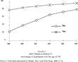
FIGURE 2 SOUTHERN LITERACY (percentage of the population over the age of 10)
INEQUALITY IN SPENDING BY RACE IN SOUTHERN STATES IN 1930
THE PROBABILITY OF NORTHERN RESIDENCE IN 1940 FOR SOUTHERN-BORN BLACKS
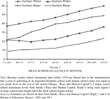
FIGURE 3 MEAN SCHOOLING LEVELS IN MONTHS
EFFECTS OF RACIAL DISCRIMINATION: STATE-LEVEL FIXED-EFFECTS REGRESSIONS, 1880–1950
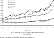
FIGURE 4 REAL ANNUAL SCHOOL EXPENDITURE PER PUPIL (1967 dollars)
FIXED-EFFECTS LEVEL REGRESSIONS, 1880–1950
FIXED EFFECTS GROWTH REGRESSIONS, 1880–1950
APPENDIX TABLE 1 RANDOM-EFFECTS ESTIMATION, 1880–1950
APPENDIX TABLE 2 RANDOM-EFFECTS ESTIMATION, 1880–1950
 You have
Access
- 15
- Cited by