1. Introduction
The study of boundary-layer transition from laminar to turbulent flow on high-speed vehicles has been the subject of ongoing research for over fifty years. This activity is indicative of the difficult but potentially rewarding nature of these efforts. In the design of hypervelocity vehicles, the location of transition critically determines not only the drag, but also the degree to which thermal protection needs to be applied, because both friction and heating rate jump significantly at the transition point (Saric, Reed & Kerschen Reference Saric, Reed and Kerschen2002; Schneider Reference Schneider2004; Lau Reference Lau2008; Lin Reference Lin2008; Reshotko Reference Reshotko2008; Schmisseur & Erbland Reference Schmisseur and Erbland2012). The receptivity and growth of the disturbances that precede transition within an initially laminar boundary layer in hypervelocity (characterized by speeds exceeding 3–
 $4~\text{km}~\text{s}^{-1}$
) flow are less understood than in subsonic flows, particularly at conditions where gas dissociation and vibrational excitation must be considered. A better understanding of the receptivity and amplification process of disturbances in the boundary layer in this flight regime would enable more precise sizing of thermal protection systems, and facilitate hypervelocity vehicle optimization.
1.1. Compressible boundary-layer instability
There are many boundary-layer configurations and mechanisms of instability that are possible on vehicles. In the present study, we focus on the simplest configuration of a streamlined body and examine the flow associated with the development of a zero-pressure-gradient laminar boundary layer away from the leading edge or interference regions. Researchers have used the sharp flat plate and right-circular cone at zero angle of attack as the canonical geometry to study high-speed boundary-layer instability; in this work, we chose the latter. We make this choice because of the larger entropy layer ‘swallowing length’ associated with a sharp plate, which is in contrast to the shorter swallowing length associated with a sharp cone (Rotta Reference Rotta1966; Stetson Reference Stetson1983).
For a streamlined body in low-speed flight with an initially laminar boundary layer, the process of ‘natural’ transition (e.g. in a flow of very low free stream disturbance level) from laminar to turbulent flow is now a classical topic in fluid dynamics that is well understood. The instability theory of Tollmien (Reference Tollmien1929) and Schlichting (Reference Schlichting1933) of the growth of unstable modes (‘T–S waves’) prior to boundary-layer transition was experimentally verified by Schubauer & Skramstad (Reference Schubauer and Skramstad1948), and subsequently has been the topic of numerous experimental, analytical and numerical studies. This is in contrast to the situation for high-speed flow with significant compressibility and thermal effects, where, despite the initial efforts of Lees & Lin (Reference Lees and Lin1946), real progress did not occur until the discovery by Mack in the 1960s of multiple high-frequency instability modes that were confirmed in the experimental measurements by Kendall at JPL; see Mack (Reference Mack, Fasel and Saric1999) for the history. The technical results of that first era of research, and the application to the prediction of supersonic boundary-layer transition are summarized in Mack (Reference Mack1975, Reference Mack1984, Reference Mack, Fasel and Saric1999).
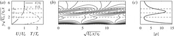
The high-frequency modes discovered by Mack are the dominant instability mechanism when the boundary-layer edge Mach number is sufficiently large, the angle of attack is small, and the wall temperature is sufficiently low compared to the recovery temperature; see the discussion and references in Bitter & Shepherd (Reference Bitter and Shepherd2014). Under these conditions the boundary layer features a region of supersonic flow relative to the phase velocity of disturbances, which acts as a waveguide and traps the disturbances within the boundary layer, leading to amplification (Fedorov Reference Fedorov2011). Linear-stability theory predicts that waves of wavelength two to three times the boundary-layer thickness will propagate and amplify if the frequency is within a narrow range determined by the dispersion relation. A typical pattern of density disturbances predicted by linear instability theory is shown in figure 1. This pattern convects with a velocity close to the edge value, and the spatial growth rate is inversely proportional to the boundary-layer thickness (Bitter Reference Bitter2015). The presence of these propagating disturbances can be measured by a variety of means, as discussed subsequently (§ 2), and the analysis of the frequency content, propagation speed and amplitude can be used to experimentally characterize boundary-layer instability.
(a) Velocity and temperature profile in the boundary layer as a function of wall-normal distance
 $y$
. Flow of nitrogen with
 $\mathit{Re}_{x}=1.83\times 10^{6}$
,
 $Ma_{E}=5.93$
, a cold (300 K) wall and a warm (1014 K) free stream. (b) Contours of the real part of the density eigenfunction for a growing disturbance corresponding to Mack’s second mode; this pattern propagates past a fixed measurement point
 $x$
with phase speed
 $c=0.9U_{E}$
for this particular case. The eigenfunctions are normalized so that the amplitude of the pressure disturbance at the wall is unity. The location where the disturbance phase speed
 $c=U$
is known as the critical layer and the location
 $c=U+a$
(
 $a$
being the local sound speed) is known as the disturbance relative sonic line. (c) Amplitude of density eigenfunction. These computations are based on locally parallel flow theory using the method of Mack for spatial instability (Bitter & Shepherd Reference Bitter and Shepherd2014).

Mack termed the dominant higher-frequency mode the ‘second mode’, but Fedorov & Tumin (Reference Fedorov and Tumin2011) suggest ‘that Mack’s definitions of modes are inconsistent with conventional usage of the term normal modes’. Careful examination of the mode structure in the mathematical sense reveals that the instabilities arise from either fast or slow eigenmodes, as categorized by their phase speed at low frequency. However, most researchers continue to use the terminology ‘second mode’ to refer to the most rapidly growing of the Mack instability modes, to differentiate these from other possible boundary instabilities such as TS waves, crossflow, or transient-growth mechanisms. We will continue to use the historical terminology of ‘second mode’ in this paper.
1.2. Hypervelocity flow
Hypervelocity flows are distinguished by not only having a high Mach number (
 $Ma_{E}\geqslant 5$
), but also having a flow velocity
 $U$
that is large enough so that significant vibrational excitation and dissociation can occur behind bow shocks and within boundary layers (Stalker Reference Stalker1989). These processes are known as ‘real gas’ or ‘high-enthalpy’ effects due to the magnitude of the mass-specific total enthalpy,
 $h_{0}=h+U^{2}/2$
(Hornung Reference Hornung1993). The mass-specific total enthalpy plays a key role in the conversion of flow kinetic energy into thermal, vibrational and chemical energy in stagnation-like processes that exhibit a significant gradient in velocity (e.g. blunt-body flows, or slender-body viscous flows). For example, flows with
 $U=3~\text{km}\,\text{s}^{-1}$
and
 $6~\text{km}\,\text{s}^{-1}$
correspond to energies
 $(U^{2}/2)$
of
 $4.5~\text{MJ}\,\text{kg}^{-1}$
and
 $18~\text{MJ}\,\text{kg}^{-1}$
, respectively. The ability to achieve these energies is the principal advantage of using the reflected-shock tunnel with heated driver gas over conventional cold-flow hypersonic facilities.
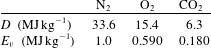
The characteristic energies of dissociation (
 $D$
) and vibrational excitation (
 $E_{v}$
) for N2,O2 and CO2 are listed in table 1. For carbon dioxide, the dissociation reaction
 $\text{CO}_{2}\rightarrow \text{CO}+\frac{1}{2}\text{O}_{2}$
, and the lowest-energy (doubly degenerate) mode of vibrational excitation are considered. From these values, we see that significant vibrational excitation will occur for all of these molecules at and above
 $3~\text{km}\,\text{s}^{-1}$
. At higher speeds the dissociation of oxygen and carbon dioxide will be significant. Nitrogen will remain primarily in the molecular form at speeds up to
 $6~\text{km}\,\text{s}^{-1}$
for typical test conditions simulating suborbital flight.
Characteristic energy of dissociation
 $D$
and vibration
 $E_{v}$
(McQuarrie Reference McQuarrie2000).

The influence of molecular vibrational excitation and dissociation on the transition from laminar to turbulent flow depends not only on the magnitude of the total enthalpy but also the rate of energy exchange between molecular processes and bulk motion. There are two possible effects: (1) the modification of the mean flow due to energy release or absorption modifying the temperature profile; and (2) the exchange of energy between the high-frequency second-mode instability of a hypersonic boundary layer and molecular vibrational relaxation or chemical relaxation processes. Linear-stability computations (Johnson, Seipp & Candler Reference Johnson, Seipp and Candler1998) indicate that endo- or exothermic chemical-thermodynamic processes affect the growth of small disturbances in the boundary layer. For this reason, we have examined three test gases, air, nitrogen and carbon dioxide, and a range of total enthalpy.
At sufficiently high Mach number there are also significant effects on the mean flow that can substantially influence the boundary-layer stability through the resulting mean temperature profile. Viscous dissipation results in the transformation of kinetic to thermal energy within the boundary layer, so the temperature within the boundary layer can be substantially higher than the free stream value. The shape of the temperature profile is a function of the boundary-layer edge conditions, the duration of the test, and the thermal properties of the model. The temperature-profile gradient at the model wall dictates whether a ‘cold wall’, ‘adiabatic wall’, or ‘hot wall’ experiment is being performed. For high-enthalpy short-duration experiments with a hot free stream, typical of reflected-shock or expansion tunnel testing, the model remains cold; so, the data reported herein are from cold-wall experiments. Calculations of the boundary-layer flow indicate that there is a pronounced temperature maximum within the boundary layer, as shown in figure 1. Stability computations (Mack Reference Mack1975, Reference Mack1984, Reference Mack, Fasel and Saric1999; Bitter & Shepherd Reference Bitter and Shepherd2014; Bitter Reference Bitter2015) indicate that the shape of the mean temperature profile has a profound influence on the stability characteristics of the boundary layer. A cold wall stabilizes the first mode and destabilizes the second mode; at sufficiently high edge Mach number and wall cooling, the first mode is completely eliminated.
2. Measurement of second-mode instability
Measurements of the instability of the boundary layer on a sharp right-circular cone at zero angle of attack at hypersonic Mach numbers have been made with a number of measurement techniques. Kendall (Reference Kendall1975), Demetriades (Reference Demetriades1977) and Stetson et al. (Reference Stetson, Thompson, Donaldson and Siler1983), Stetson, Donaldson & Siler (Reference Stetson, Donaldson and Siler1984), Stetson et al. (Reference Stetson, Thompson, Donaldson and Siler1989) appear to have made the first measurements of the Mack instability with hot-wire anemometry. Demetriades observed that the frequency of the instability,
 $f$
, is proportional to the velocity at the boundary-layer edge,
 $U_{E}$
, and inversely proportional to the boundary-layer thickness,
 ${\it\delta}$
:
 $f=CU_{E}/(2{\it\delta})$
, where the constant of proportionality is
 $0.6<C<0.9$
. In Kimmel, Demetriades & Donaldson (Reference Kimmel, Demetriades and Donaldson1996), extensive circumferential, streamwise, and wall-normal space–time correlations of detailed hot-wire anemometry data are used to characterize the structure of the instability waves. Hofferth et al. (Reference Hofferth, Humble, Floryan and Saric2013a
,Reference Hofferth, Saric, Kuehl, Perez, Kocian and Reed
b
) recently carried out an extensive series of hot-wire measurements of mean flow and fluctuations within the boundary layer of a flared cone in a ‘quiet flow’ Mach 6 tunnel.
Commercial piezo-electric pressure transducers have been used recently by a number of investigators, mounting these flush with the surface of the test article to record wall-pressure fluctuations due to the boundary-layer instability. Fujii (Reference Fujii2006) used pressure transducers placed along a generator of a 5° half-angle cone to assess the effect of a wavy-wall roughness on the growth of the boundary-layer instability. Fujii et al. (Reference Fujii, Noriaki, Tadao, Shoichi, Muneyoshi, Yukihiro, Akihiro and Hiroshi2011) used surface-mounted pressure transducers to measure the second-mode instability and its growth rate along a generator of the cone; additionally, the nonlinear phase coupling of the disturbances was analysed by the bicoherence method. Casper (Reference Casper2009) and Berridge (Reference Berridge2010) made hypersonic boundary-layer instability measurements with piezo-electric pressure transducers in a low-disturbance hypersonic facility. Typically, these measurements are limited to frequencies less than 300–500 kHz. The frequency response of the transducers is difficult to accurately characterize; although, the intrinsic resonant frequency of the transducers is quoted to be of the order of 1 MHz.
Fast-response heat-flux gauges have also been utilized to measure the high-frequency fluctuations in a hypersonic boundary layer. The atomic layer thermopile (ALTP) developed by Roediger et al. (Reference Roediger, Knauss, Gaisbauer, Kraemer, Jenkins and von Wolfersdorf2008) is claimed to have a frequency response of up to 1 MHz. Roediger et al. (Reference Roediger, Knauss, Estorf, Schneider and Smorodsky2009) utilized ALTP gauges to measure the second-mode instability waves and compared the experimentally observed growth rates to growth rates calculated from linear-stability theory. Heitmann et al. (Reference Heitmann, Kähler, Radespiel, Rödiger, Knauss and Wagner2011) used such heat-flux gauges to measure instabilities that were artificially excited in a hypersonic boundary layer.
For high-frequency measurements and locations within the boundary layer rather than on the model surface, optical methods are more promising than pressure or heat-flux transducers. A schlieren-based technique for the investigation of disturbances has been reported (Laurence et al. Reference Laurence, Wagner, Hannemann, Wartemann, Lüdeke, Tanno and Itoh2012; Laurence, Wagner & Hannemann Reference Laurence, Wagner and Hannemann2014a ; Laurence et al. Reference Laurence, Wagner, Ozawa, Schramm and Hannemann2014b ). In those reports, high-resolution and time-resolved images of the second-mode instability structure, along with valuable spectral and cross-correlation data are presented. Additionally, an optical technique based on a grid and lens style focused-schlieren technique was developed by Boedeker (Reference Boedeker1959) and refined by Weinstein (Reference Weinstein1993) and Garg & Settles (Reference Garg and Settles1998). VanDercreek (Reference VanDercreek2010) and VanDercreek, Smith & Yu (Reference VanDercreek, Smith and Yu2010) used this technique in their research, making measurements of the second-mode instability with the focused-schlieren deflectometer as well as with piezo-electric pressure transducers. Resonantly enhanced focused-schlieren measurements in T5 yielded some promising results (Parziale et al. Reference Parziale, Jewell, Shepherd and Hornung2011). Peaks in the spectral content at frequencies consistent with the Mack mode instability were found along with detection of turbulent bursts; however, the method of resonantly enhanced focused schlieren makes quantitative interpretation of the results difficult. Hofferth et al. (Reference Hofferth, Humble, Floryan and Saric2013a ,Reference Hofferth, Saric, Kuehl, Perez, Kocian and Reed b ) used the focused-schlieren technique to measure the second-mode waves in a low-disturbance wind tunnel.
Another very promising optical method is the two-beam laser differential interferometry (LDI) technique that was used to experimentally characterize gas-dynamic flows by Smeets and George at the French–German Research Institute of Saint-Louis (ISL) in the 1970s (Smeets Reference Smeets1972, Reference Smeets1973, Reference Smeets1974, Reference Smeets1977; Smeets & George Reference Smeets and George1973). The technique is sensitive to changes in optical path length that are related to density by the Gladstone–Dale relation. Smeets and George designed many variants of the two-beam differential interferometer, which were cleverly applied to demonstrate the potential of this approach in non-steady gas-dynamics, steady compressible aerodynamics, and acoustics.
Laderman & Demetriades (Reference Laderman and Demetriades1976) used the LDI method as a boundary-layer transition detection tool at Mach 3; they used a line-of-sight integrating LDI to detect increases in the RMS fluctuations in the boundary layer and related the increases in RMS fluctuation to transition to turbulence. Azzazy, Modarress & Hoeft (Reference Azzazy, Modarress and Hoeft1987) discusses the LDI as a turbulence detection tool in a shear layer, on a wind-tunnel wall at low subsonic Mach number, and in a Mach 2.36 boundary layer. They made measurements of transition in the shear layer and on the subsonic wind-tunnel wall, resolving low-frequency (
 ${<}100~\text{kHz}$
) spectral content. The LDI in O’Hare (Reference O’Hare1985) was a line-of-sight integrating set-up that imaged a shift in the fringe pattern formed on a wind-tunnel wall by two beams, one of which probed the hypersonic boundary layer on a slender cone, the other traversed the mean flow outside of the boundary layer. Frequencies in the range of the anticipated second-mode values were observed with the LDI, and were consistent with hot-wire anemometry, although the SNR was poor, and the frequency response appeared to be limited to less than
 $200~\text{kHz}$
. Salyer, Collicott & Schneider (Reference Salyer, Collicott and Schneider2006) used an LDI to make measurements in front of and behind the bow shock on a hemisphere for a hot spot generated by laser breakdown in a Mach 4 flow. Because the interest was in receptivity, all measurements were made outside the boundary layer.
It is significant that most of the previous efforts in measuring disturbances associated with the second-mode instability have been carried out in steady or quasi-steady flow facilities in relatively low vibration environments. The flows are typically relatively cold (low enthalpy) flows in which great attention (Schneider Reference Schneider2008) is paid to upstream flow quality and elimination of particulate matter in the flow, nozzle boundary-layer transition suppression, and, in general, efforts to make the tunnel as ‘quiet’ as possible. This is in contrast to the harsh mechanical environment of reflected-shock tunnels like T5. However, given the success of past efforts (Adam & Hornung Reference Adam and Hornung1997; Germain & Hornung Reference Germain and Hornung1997; Rasheed et al. Reference Rasheed, Hornung, Fedorov and Malmuth2002) in T5, as well as other researchers using shock tunnels (Tanno et al. Reference Tanno, Komura, Sato, Itoh, Takahashi and Fujii2009; Laurence et al. Reference Laurence, Wagner, Hannemann, Wartemann, Lüdeke, Tanno and Itoh2012, Reference Laurence, Wagner and Hannemann2014a ,Reference Laurence, Wagner, Ozawa, Schramm and Hannemann b ) to study stability and transition, we felt confident that measurement solutions could be found.
2.1. Focused laser differential interferometry
Measurement of small-amplitude disturbances characteristic of the second-mode instability is a challenging task for a large-scale hypervelocity ground-test facility like T5. Considering the operation of the facility and the expected characteristics of the Mack mode disturbances, we identified six requirements for the instrumentation: (1) high sensitivity to small flow disturbances within the boundary layer; (2) high temporal resolution (
 ${>}10~\text{MHz}$
); (3) high spatial resolution to resolve the small wavelength of the disturbance (
 ${<}1~\text{mm}$
); (4) insensitivity to mechanical vibration; (5) the capability to have a small focal volume near the surface of the cone; and (6) a straightforward and repeatable means of extracting quantitative data. After experimenting with a number of techniques, Parziale, Shepherd & Hornung (Reference Parziale, Shepherd and Hornung2013b
, Reference Parziale, Shepherd and Hornung2014) demonstrated that focused laser differential interferometry (FLDI) meets all these requirements.
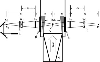
The principle of the particular FLDI set-up used in the present study is to create two focal volumes within the boundary layer that are separated by a distance that is smaller than the wavelength of the density disturbance (figure 2). The key idea is to detect differences in optical path length due to the density differences at the two focal regions spatially separated in the streamwise direction. The other key distinguishing feature of the present set-up is that the optical paths of the light used to form the two focal volumes closely overlap except for a small region around the separated focal volumes. The geometry of the light paths ensures the localization of the probe volume, and rejection of disturbances common to both paths. The high speed of measurement is due to the intrinsic high-frequency response of the electro-optical detectors and recording equipment. All of these features were key to enabling the measurements under T5 conditions.
Annotated schematic of the FLDI. TSL, turbulent shear layer, L, Laser; M, mirror;
 $C_{1}$
, 10 mm focal length lens;
 $C_{2}$
, 300 mm focal length lens; P, polarizer; W, Wollaston prism (2 arc minutes); B, BK7 window; A, probe volume; D, photodetector; N, nozzle,
 $s_{1}=718~\text{mm}$
,
 $s_{2}=515~\text{mm},s_{3}=300~\text{mm}$
.

The laser used in this experiment is a Spectra-Physics Excelsior diode pumped solid state continuous-wave laser (532 nm wavelength, 200 mW power). The high-quality beam (
 $\text{TEM}_{00}$
) does not require additional beam conditioning for use as an interferometer. A schematic of the optical set-up is presented in figure 2. The response of the photodetector (22.5 V battery biased FDS100 photodiode) is amplified at a gain of 25 (SRS SR445) and digitized at 100 MHz by a 14-bit Ethernet oscilloscope (Cleverscope CS328A-XSE); all leads are terminated at
 $50~{\rm\Omega}$
.
A relationship between the fluctuations in density and output voltage from the photodetector is required for interpreting the FLDI output, and is determined (Parziale et al. Reference Parziale, Shepherd and Hornung2013b ) to be
 $$\begin{eqnarray}\frac{{\rm\Delta}{\it\rho}}{{\it\rho}_{L}}=\frac{{\it\lambda}_{0}}{2{\rm\pi}KL{\it\rho}_{L}}\sin ^{-1}\left(\frac{V}{V_{0}}-1\right).\end{eqnarray}$$
This relation is found by considering the variations in optical phase along the beam direction,
 $z$
, and considering the FLDI as a two-beam differential interferometer. Here,
 ${\rm\Delta}{\it\rho}/{\it\rho}_{L}$
is the difference in density traversed by the sensitive probe volumes normalized by the local average density. The laser wavelength is
 ${\it\lambda}_{0}$
,
 $K$
is the Gladstone–Dale constant,
 $V$
is the instantaneous photodetector voltage,
 $V_{0}$
is the photodetector voltage at the middle of an interference fringe, and
 $L$
is the sensitive length. The sensitive length was determined to be approximately
 $\pm 10~\text{mm}$
from the beam focus. This was found by utilizing a steady CO2 jet as a control, and traversing a distance from the beam focus to determine the point at which the response is decreased by
 $1/e$
from the centreline value (Parziale, Shepherd & Hornung Reference Parziale, Shepherd and Hornung2013a
; Parziale Reference Parziale2013). Additionally, spherical acoustic pulses were created by focusing a 200 mJ 532 nm Nd:YAG laser to ionize a small volume of gas equidistant from the upstream and downstream detectors. The difference in peak response for properly aligned systems is less than
 $3.5\,\%$
, bringing confidence to the repeatability of the experiment. This testing procedure is repeated approximately every 20 T5 shots, or when the results from the previous T5 shot indicate misalignment (Parziale et al.
Reference Parziale, Shepherd and Hornung2013a
; Parziale Reference Parziale2013).
The two beams are spaced
 $350~{\rm\mu}\text{m}$
apart in the streamwise direction, and the phase object is integrated over the optical path length
 $L$
. It is clear that some averaging of the density variations across the boundary layer will take place due to the finite width of the sensitive volume in the spanwise direction. However, due to the two-dimensional nature of the Mack modes (Mack Reference Mack1975, Reference Mack1984, Reference Mack, Fasel and Saric1999) and the rapid decrease in detection sensitivity with increasing transverse distance from the focal point, the average density difference is highly weighted towards the values near the focal volumes.
For each individual T5 test, the wall-normal distance from the surface of the cone to the volume being probed by the FLDI is measured with a dial-indicator, translating a razor-blade cutoff normal to the surface of the cone. Wall-normal distances range from 450–
 $990~{\rm\mu}\text{m}$
, and the uncertainty is estimated to be
 $\pm 50~{\rm\mu}\text{m}$
; this is the calculated beam diameter, which is noted to be twice the precision of the dial-indicator. The wall-normal distance is chosen to be approximately 60 % of the predicted boundary-layer thickness at each probe-volume location. There were two FLDI probe volumes used to simultaneously measure the instability at two locations within the boundary layer; they were located
 $627\pm 1~\text{mm}$
and
 $718\pm 1~\text{mm}$
from the cone tip along a single cone generator.
The systematic error stemming from applying (2.1) to the raw data is found by considering the propagation of uncertainty in
 ${\rm\Delta}{\it\rho}/{\it\rho}_{L}$
as a function of all the input parameters, assuming that they are independent of each other (Coleman & Steele Reference Coleman and Steele1999). The error in
 ${\rm\Delta}{\it\rho}/{\it\rho}_{L}$
is approximately 20 %. Details of the error analysis are reported in Parziale et al. (Reference Parziale, Shepherd and Hornung2013b
).
3. T5 testing and results
A series of tests in the T5 reflected-shock tunnel are carried out to measure the incipient instability waves prior to the transition to fully turbulent flow on a right-circular cone at zero angle of attack. The 5° half-angle cone is constructed of aluminium and instrumented with an array of flush-mounted fast-response thermocouples used as heat-flux gauges; the heat-flux gauges are used to determine the transition location, as determined by the departure from calculated laminar heating rate. The cone has a surface roughness of less than
 $5~{\rm\mu}\text{m}$
and has a replaceable molybdenum tip that has a radius estimated to be
 $400~{\rm\mu}\text{m}$
; after a break-in period for a new tip, this radius remains essentially constant during the testing series. The slightly blunt tip produces a bow shock, resulting in the boundary layer initially developing within the hot, high-entropy fluid layer downstream of the bow shock. In the flow over a cone, the entropy layer decreases with downstream distance until it is eventually ‘swallowed’ by the boundary layer. Following Rotta (Reference Rotta1966) and Stetson (Reference Stetson1983), the ‘swallowing’ distance is calculated to be no more than 90 mm from the cone tip for any run condition presented in this work. This distance is less than 15 % of the distance to the upstream FLDI probe volume; therefore, the cone is idealized as ‘sharp’ for the purposes of analysing the outer flow and the boundary layer at the probe-volume locations.
The tunnel operation and data analysis are described in detail by Parziale (Reference Parziale2013). Briefly, the shock tunnel uses an air-driven piston to create hot, high-pressure driver gas to rupture the primary diaphragm and produce a strong shock wave in the test gas. The reflection of the shock at the end of the shock tube generates the high-enthalpy reservoir used to supply a converging–diverging nozzle; quasi-steady flow in the nozzle creates the hypervelocity flow over the cone model located near the nozzle exit. The noise level in the free stream flow is characterized using single-point FLDI density fluctuation measurements in the free stream, as discussed in Parziale et al. (Reference Parziale, Shepherd and Hornung2014). The typical RMS fluctuation intensity is less than 0.5 % for disturbance wavelengths between 0.7 and 10 mm, the range relevant to direct excitation of second-mode instabilities in our study. The fluctuation intensity is higher (up to 5–7 %) at longer wavelengths, up to 100 mm, which may be relevant to various receptivity mechanisms; a review of nonlinear breakdown processes in hypersonic boundary layers can be found in Zhong & Wang (Reference Zhong and Wang2012).
A range of flow conditions can be generated at the nozzle exit by varying the gas composition and fill pressures in the shock tube and driver, as well the primary diaphragm rupture pressure. Relying on an extensive database from past operation and calibration of the tunnel performance, the flow Reynolds number and location of transition to turbulence on the cone model can be adjusted so that repeatable observations can be made of the onset and growth of instabilities in an initially laminar boundary layer. The location of boundary-layer transition is identified by departure from laminar surface heat-flux rates measured by surface-mounted heat-transfer gauges, as discussed in Jewell et al. (Reference Jewell, Leyva, Parziale and Shepherd2011, Reference Jewell, Parziale, Leyva, Shepherd and Hornung2012), Jewell, Shepherd & Leyva (Reference Jewell, Shepherd and Leyva2013a
), Jewell et al. (Reference Jewell, Wagnild, Leyva, Candler and Shepherd2013b
) and Jewell (Reference Jewell2014). Operating conditions for T5 are selected on the basis of these heat-flux measurements and, more importantly, the FLDI measurements provided a clear indication of the nature of the flow at those measurement locations. Through careful selection of conditions and cleaning of the shock tube, it is possible to systematically prescribe transition locations that are estimated to correspond to second-mode amplification factors
 $e^{N}$
of
 $N\approx 8{-}12$
(Jewell et al.
Reference Jewell, Shepherd and Leyva2013a
,Reference Jewell, Wagnild, Leyva, Candler and Shepherd
b
; Jewell Reference Jewell2014). These amplification values are high as compared to the more typical value of
 $N\approx 5{-}6$
usually characterizing a ‘noisy’ tunnel (Schneider Reference Schneider2001), but consistent with the expected difference in receptivity for the high-frequency second-mode instability as compared to the relatively low-frequency noise in the T5 free stream as measured by Parziale et al. (Reference Parziale, Shepherd and Hornung2014). This is supported by the recent analysis of Gronvall, Johnson & Candler (Reference Gronvall, Johnson and Candler2014), who found a transition onset value of
 $N\sim 8$
for the shock-tunnel experiments of Tanno et al. (Reference Tanno, Komura, Sato, Itoh, Takahashi and Fujii2009).
For each test, the flow conditions at the outer edge of the boundary layer are computed using measured tunnel data and numerical simulation of the shock reflection process, flow through the nozzle, and over the cone model. The measured shock speed and reflected-shock pressure are used to obtain the conditions in the reservoir following shock reflection based on equilibrium thermochemistry, the shock jump conditions, and assuming isentropic expansion of the gas at the end wall to the pressure measured during the test time. An accurate geometric model of the converging–diverging nozzle is used to compute the steady expansion of the reservoir gas, including real gas effects through an excluded volume model, as described by Candler (Reference Candler2005). Averaged conditions on the centreline of the nozzle at the cone tip are used as the input to compute the viscous flow over the cone. Both the nozzle and cone flow simulations assume axisymmetric viscous flow, and include chemical reaction and vibration-translational rate processes. The computations were carried out with the STABL software suite, which uses a data-parallel lower-upper relaxation (DPLR) method, as described by Wright, Candler & Prampolini (Reference Wright, Candler and Prampolini1996), Johnson et al. (Reference Johnson, Seipp and Candler1998), and Johnson (Reference Johnson2000).
3.1. FLDI measurements
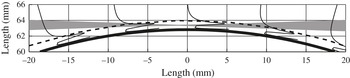
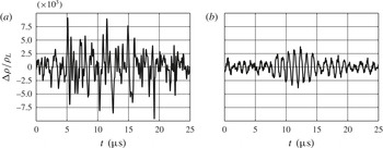
Two FLDI measurement volumes, located within the boundary layer (figure 3) and upstream of the transition location, are used to simultaneously measure time-resolved density fluctuations. Representative principal signatures observed in FLDI signals are shown in figure 4. The signal in (a) represents a large-amplitude, broad-band disturbance that is associated with locally turbulent flow, whereas that in (b) represents a small-amplitude, narrow-band disturbance in otherwise laminar flow. We will refer to these distinct signatures in subsequent descriptions of experimental results. We interpret the large-amplitude signature (a) as corresponding to the passage of a turbulent spot past the measurement location. The small-amplitude signature (b) corresponds to the passage of a second-mode wavepacket.
Overlay of cone surface (solid thick line), calculated boundary-layer thickness for shot 2789 (dashed line), density eigenfunction for shot 2789 (solid thin lines), and laser beam profile (grey filled area). The zero of the abscissa is the focus of the beam. The cone tip is located out of the page.

Examples of the two principal signatures observed in FLDI signals: (a) broad-band, large-amplitude signal characteristic of locally turbulent flow; (b) narrow-band, small-amplitude signal, characteristic of a wavepacket in laminar flow. These examples are for an air boundary layer (shot 2743) with
 $h=9.1~\text{MJ}\,\text{kg}^{-1}$
.

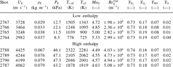
Air boundary-layer edge conditions.

Results of the FLDI time series measurements are analysed in terms of frequency content, coherence of upstream and downstream disturbances, and the change in disturbance amplitude between the two locations. Measurements were made in air for two ranges of total enthalpy, in nitrogen for three ranges of total enthalpy, and in carbon dioxide for one range of total enthalpy. The results for air are presented in detail, and the results for the N2 and CO2 are described more briefly, as the measured spectral content was qualitatively similar for all test gases. In addition to the FLDI measurements, high-speed video recording of the density disturbances are made for selected cases.
There are two series of air tests, described in
 $\,$
table 2
 $\,$
as
 $\,$
‘low
 $\,$
enthalpy’
 $\,$
(
 $5{-}9~\text{MJ}\,\text{kg}^{-1}$
) and ‘high enthalpy’ (
 $11{-}13~\text{MJ}\,\text{kg}^{-1}$
). The rapid expansion in the shock-tunnel nozzle results in boundary-layer edge conditions that are slightly out of equilibrium due to the ‘freezing’ of both chemical reactions and exchange of energy between vibrational modes of molecular motion and the translational and rotational modes. This results in the effective translational–rotational temperature
 $T_{t/rE}$
being slightly (50–150 K) lower than the effective vibrational temperature
 $T_{vE}$
. The air is highly dissociated upstream of the shock-tunnel nozzle, and the freezing of the recombination reactions during flow through the nozzle results in a significant (7–8 %) non-equilibrium concentration of NO and a smaller (1–2 %) amount of O, as indicated by the mass fractions
 $Y_{\text{NO}}$
and
 $Y_{\text{O}}$
. The same nozzle is used for all tests so that the edge Mach number
 $Ma_{E}$
is nearly constant for the low enthalpy and high enthalpy test series, varying because of thermochemical and real gas effects, resulting in slightly off-design operation that depends on the particular conditions of each case.
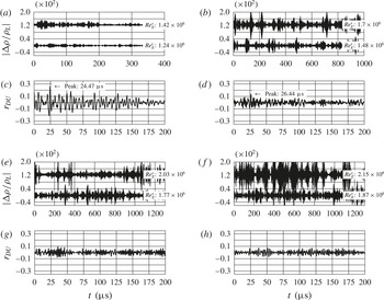
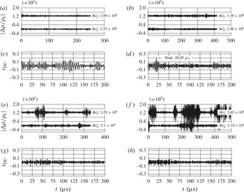
(a,b,e,f) Time traces and (c,d,g,h) cross-correlations of
 ${\rm\Delta}{\it\rho}/{\it\rho}_{L}$
for the low-enthalpy air test series (conditions summarized in table 2). In order of increasing unit Reynolds number: (a,c) Shot 2767 –
 $\mathit{Re}_{E}^{Unit}=1.98\times 10^{6}~\text{m}^{-1}$
; (b,d) Shot 2766 –
 $\mathit{Re}_{E}^{Unit}=2.36\times 10^{6}~\text{m}^{-1}$
; (e,g) Shot 2765 –
 $\mathit{Re}_{E}^{Unit}=2.82\times 10^{6}~\text{m}^{-1}$
; (f,h) Shot 2764:
 $\mathit{Re}_{E}^{Unit}=2.99\times 10^{6}~\text{m}^{-1}$
.

In each series, the unit Reynolds number (
 $\mathit{Re}_{E}^{Unit}$
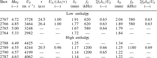
) is evaluated at the boundary-layer edge, and decreases when the reservoir pressure is held nominally constant and the reservoir enthalpy is increased. This leads to the somewhat counterintuitive result that in order to move the transition location forward under constant reservoir pressure conditions, the reservoir enthalpy is lowered. The primary difference in edge conditions between low- and high-enthalpy tests is the magnitude of the edge flow speed and temperature – both are increasing functions of reservoir enthalpy. In order to compensate for the decrease in Reynolds number with increasing reservoir enthalpy, and obtain transition at similar physical locations in both series of tests, the reservoir pressure was adjusted to be higher in the high-enthalpy series than in the low-enthalpy series. The high-enthalpy cases have boundary layers that are approximately 60 % thinner than for the low-enthalpy cases. Thinner boundary layers combined with higher edge speeds result in second-mode frequencies that are approximately twice as high for the high-enthalpy as compared to low-enthalpy cases.
3.1.1. Low-enthalpy conditions
Segments of time series of non-dimensional fluctuations in density (
 ${\rm\Delta}{\it\rho}/{\it\rho}_{L}$
) at both probe volumes and cross-correlation of the upstream and downstream signals are shown in figure 5 for four values of unit Reynolds number. These signals have been band-pass filtered to remove low- and high-frequency noise; the frequency band has been selected to bracket the range of frequencies characterizing second-mode instabilities. The density fluctuations shown in figure 5 increase in amplitude between the upstream (lower signal) and downstream locations (upper signal), and the RMS signal level at both locations increases with increasing unit Reynolds number. Although details of the waveforms shown in figure 4 cannot be observed in figure 5 due to the much longer time scale, it is clear that the signals are made up of ‘bursts’ occurring at irregular intervals, characteristic of fluctuations observed in flows near the onset of turbulence.
The cross-correlations in figure 5 are normalized by the square root of the product of the auto-covariances at zero lag, so that the maximum correlation value is unity. A distinct correlation peak near
 $25~{\rm\mu}\text{s}$
can be observed for the two low-Reynolds-number cases, figure 5(a,c) and (b,d). A pronounced peak in cross-correlation is observed when both the upstream and downstream signals show the low-amplitude, wavepacket-like signature of figure 4(b). The time
 ${\it\tau}$
corresponding to the peak in the cross-correlation is within 5 % (table 3) of the time
 ${\rm\Delta}s/U_{E}$
, where
 $U_{E}$
is the boundary-layer edge velocity and
 ${\rm\Delta}s$
is the distance between the detector locations. This suggests that the detectors are tracking wavepackets that are travelling along the generator of the cone at approximately the edge velocity. Further examination of the signals shows that the well-defined peak in the cross-correlation occurs only when both detectors have a distinct narrow-band spectral response corresponding to signals composed primarily of wavepackets of the type in figure 4(b). No well-defined cross-correlation peak is observed in either figure 5(e,g) or (f,h), as the downstream detector signals consist primarily of broad-band disturbances with the signature of figure 4(a).
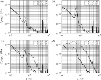
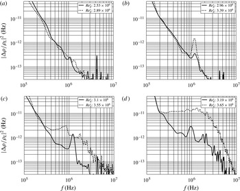
Power spectral density estimates of
 ${\rm\Delta}{\it\rho}/{\it\rho}_{L}$
for the low-enthalpy air shot series (conditions summarized in table 2). In order of increasing unit Reynolds number: (a) shot 2767 –
 $\mathit{Re}_{E}^{Unit}=1.98\times 10^{6}~\text{m}^{-1}$
; (b) shot 2766 –
 $\mathit{Re}_{E}^{Unit}=2.36\times 10^{6}~\text{m}^{-1}$
; (c) shot 2765 –
 $\mathit{Re}_{E}^{Unit}=2.82\times 10^{6}~\text{m}^{-1}$
, shot 2764: (d)
 $\mathit{Re}_{E}^{Unit}=2.99\times 10^{6}~\text{m}^{-1}$
.

Air boundary-layer instability parameters and scaling.

The conclusions regarding the spectral characteristics of the signals are quantitatively demonstrated by the estimates of the power spectral density (PSD) shown in figure 6 for the signals displayed in figure 5. These are computed using Welch’s method, with 50 % overlapping
 $20~{\rm\mu}\text{s}$
Hann windows. For the lowest Reynolds number cases, figure 6(a,b), distinct peaks corresponding to the wavepackets occur near a frequency of 600–700 kHz and are observed on both the upstream and downstream detectors. The peak frequency is slightly lower for the downstream signal than the upstream signal. As discussed subsequently, this is due to the increasing thickness of the boundary layer and scaling of the most unstable disturbance frequency with the reciprocal of the boundary-layer thickness.
As the Reynolds number is increased, the flow begins to transition from laminar to turbulent at the downstream detector location. The narrow-band spectral peak in the downstream signal is observed to increase in amplitude and become broader, as shown in figure 6(c). With further increases in Reynolds number, as shown in figure 6(d), the downstream spectrum increases even further in amplitude, and is spread over a broad range of frequencies with no distinct peaks. This behaviour is consistent with a fluid-dynamic instability increasing in amplitude and then breaking down to turbulence. This conclusion is supported by simultaneous measurements using surface-mounted heat-transfer gauges (Jewell et al. Reference Jewell, Leyva, Parziale and Shepherd2011, Reference Jewell, Parziale, Leyva, Shepherd and Hornung2012, Reference Jewell, Shepherd and Leyva2013a ,Reference Jewell, Wagnild, Leyva, Candler and Shepherd b ; Jewell Reference Jewell2014) which show a corresponding departure from laminar surface heat-flux rates near the downstream detector.
3.1.2. High-enthalpy conditions
A second series of shots (2788–2787) was conducted at higher reservoir pressure and reservoir enthalpy (
 $11{-}13~\text{MJ}\,\text{kg}^{-1}$
) with conditions listed in table 2. Time traces and correlations are included for these experiments in figure 7, and power spectral density estimates are shown in figure 8. The trends are qualitatively similar to the low-enthalpy series with increasing Reynolds number, resulting in a transition from narrow-band disturbances upstream to broad-band disturbances downstream. Quantitatively, the frequency of the narrow-band disturbances is approximately 1.2 MHz, which required using a smaller window (
 $10~{\rm\mu}\text{s}$
) in PSD estimates. Although the results are qualitatively similar to the low-enthalpy cases, we found it more difficult to create high-enthalpy test conditions where wavepackets can be observed at both upstream and downstream locations. As a consequence, a distinct wavepacket signature in both locations can be observed only in shot 2789, as shown in figures 7 and 8(b). Again, the narrow-band peaks observed in the spectral estimates from the low- and high-enthalpy conditions are consistent with the instability mode first described by Mack (Reference Mack1984), for which an estimate of the most strongly amplified frequency is
 $f\approx CU_{E}/(2{\it\delta})$
, where
 $C$
is approximately 0.6 to 0.7. The observations (table 3) are consistent with the predicted dependence on both boundary-layer thickness and velocity.
(a,b,e,f) Time traces and (c,d,g,h) cross-correlations of
 ${\rm\Delta}{\it\rho}/{\it\rho}_{L}$
for the high-enthalpy air shot series. The conditions are summarized in table 2 for each test: (a,c) shot 2788:
 $\mathit{Re}_{E}^{Unit}=4.03\times 10^{6}~\text{m}^{-1}$
, (b,d) shot 2789:
 $\mathit{Re}_{E}^{Unit}=4.73\times 10^{6}~\text{m}^{-1}$
, (e,g) shot 2790:
 $\mathit{Re}_{E}^{Unit}=4.94\times 10^{6}~\text{m}^{-1}$
, (f,h) shot 2787:
 $\mathit{Re}_{E}^{Unit}=5.08\times 10^{6}~\text{m}^{-1}$
.

3.1.3. N2 and CO2 cases
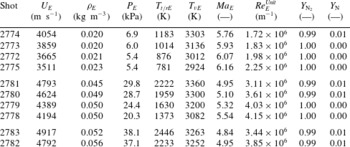
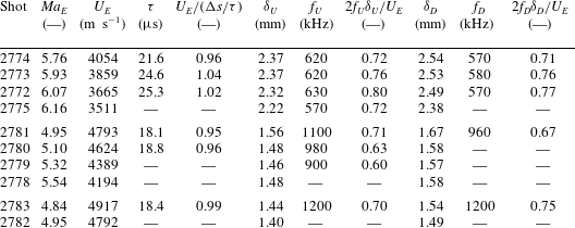
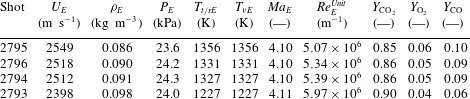
Observations using N2 and CO2 as test gases are summarized in the Appendix as tables 4–7. These results are qualitatively similar in all aspects to those obtained with air and exhibit the same quantitative scaling of the spectral peak frequency and cross-correlation of upstream and downstream signals for wavepackets. The thermochemical differences in these flows are in the extent of chemical reaction and vibrational relaxation.
There is minimal dissociation in the N2 free stream, but there is significant vibrational non-equilibrium due to slow exchange of vibrational energy with translational/rotational modes. This results in effective vibrational temperatures that are 800–2000 K higher than the translational/rotational temperature. Three ranges of reservoir enthalpy were investigated for nitrogen (low, medium and high), resulting in a range of flow speeds and non-equilibrium.
There is substantial dissociation (6–10 % CO) of the CO2 at the shock-tunnel nozzle exit, but the effective temperatures for translation/rotation and vibration are identical due to the rapid rate of energy transfer between these modes. CO2 is unique among the test gases we have examined, as it has the greatest potential for interaction of the second-mode instabilities with the molecular excitation through the energy exchange process.
Power spectral density estimates of
 ${\rm\Delta}{\it\rho}/{\it\rho}_{L}$
for the high-enthalpy air shot series. The conditions are summarized in table 2 for each of the tests: (a) shot 2788:
 $\mathit{Re}_{E}^{Unit}=4.03\times 10^{6}~\text{m}^{-1}$
, (b) shot 2789:
 $\mathit{Re}_{E}^{Unit}=4.73\times 10^{6}~\text{m}^{-1}$
, (c) shot 2790:
 $\mathit{Re}_{E}^{Unit}=4.94\times 10^{6}~\text{m}^{-1}$
, (d) shot 2787:
 $\mathit{Re}_{E}^{Unit}=5.08\times 10^{6}~\text{m}^{-1}$
.

4. Comparison of measured and predicted frequency content
Linear-stability computations were performed and compared with experimental results. The computations were carried out with PSE-Chem, a part of the STABL software package described in Johnson et al. (Reference Johnson, Seipp and Candler1998), Johnson (Reference Johnson2000), and Wagnild (Reference Wagnild2012). The mean flow over the cone is computed by DPLR (Wright et al. Reference Wright, Candler and Prampolini1996); velocity, temperature, and species concentration profiles of the boundary layer are available in chapter 2 of Parziale (Reference Parziale2013). The axis-symmetric grid for the computations was generated by the STABL package. There are 360 points in the streamwise and wall-normal directions; increasing this resolution did not yield a significant change to the baseflow. PSE-Chem analyses the mean flow over the cone. First, the method of normal modes is applied to the reacting Navier–Stokes equations, where it is assumed that the boundary layer is quasi-parallel, the gas is in thermochemical non-equilibrium, and the disturbances have the form
 $$\begin{eqnarray}q^{\prime }(s,z,t)=\hat{q}(y)\exp (\text{i}({\it\alpha}s+{\it\beta}z-{\it\omega}t)),\end{eqnarray}$$
where
 $q^{\prime }$
is a disturbance at a position along the generator of the cone
 $s$
, azimuthal position
 $z$
, and time
 $t$
. The amplitude of the disturbance is considered to be a function of only the wall-normal distance,
 $\hat{q}=\hat{q}(y)$
. The streamwise wavenumber is
 ${\it\alpha}$
, the azimuthal wavenumber is
 ${\it\beta}$
, and the angular frequency is
 ${\it\omega}$
. The spatial linear-stability problem is analysed where the frequency (
 ${\it\omega}$
) is real and the wavenumbers are complex (
 ${\it\alpha}={\it\alpha}_{r}+{\it\alpha}_{i}$
); non-zero azimuthal wavenumbers (
 ${\it\beta}$
) are not considered in this analysis, as the fastest growing disturbance is known to be two-dimensional. The results of linear-stability calculations are then used as initial values for the parabolized stability equation (PSE) analysis, which is used to account for the non-parallel nature of the boundary layer. The procedure for the PSE analysis is found in Johnson (Reference Johnson2000), which is built on the work reported in Herbert (Reference Herbert1993, Reference Herbert1997) and Chang & Malik (Reference Chang and Malik1994).
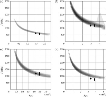
Comparisons of computational and experimental results are presented for four experiments in figure 9. For each experiment, there is a computed linear-stability diagram; the range of computed unstable frequencies is shown by the grey scale flood fill plots. The two symbols on each plot are the range of the most amplified frequencies as estimated from power spectra computed from the FLDI measurements.
Computed linear-stability diagrams and experimental spectra for four selected cases. The shaded area is the unstable region, darker shading indicates larger negative imaginary wavenumber (spatial growth rate). The circular markers represent the maximum in
 ${\rm\Delta}{\it\rho}/{\it\rho}_{L}$
from the PSD estimates, and the black line represents full-width at half-maximum of the peak in the power spectral density: (a) air low enthalpy (shot 2766); (b) air high enthalpy (shot 2789); (c) N2 high enthalpy (shot 2783); (d) CO2 (shot 2796).

There is reasonable agreement between the measured peaks in the frequency spectrum of the FLDI data and the calculated most amplified frequencies. The observed frequencies in the air and CO2 cases are systematically lower than the LST predictions at both upstream and downstream locations. If one assumes spatial growth at constant frequency (as is the case in the
 $N$
factor method), then observed peaks in the frequency spectrum should occur at higher frequencies than the calculated most amplified frequencies because of the history of growth of the packet.
This mismatch of observed and calculated frequency content may indicate that the flow is not truly two-dimensional or that there are nonlinear effects in the evolution of the wavepackets that are not accounted for by conventional LST or PSE methods.
Additionally, the inconsistency of observed and calculated content may be due to systematic error in the computed mean flow conditions at the boundary layer, associated with uncertainties in the run conditions and the physical–chemical models being used for relaxation processes as well as dissociation–recombination reactions. An approximate estimate of the change in most strongly amplified frequency (
 $f$
) due to a change in static thermodynamic conditions and velocity can be obtained by using the scaling
 $f\approx U_{E}/(2{\it\delta})$
and the correlation found for the boundary-layer thickness found in Parziale (Reference Parziale2013). Estimating the fractional change in
 $f$
as
 $\text{d}f/f=\text{d}\ln f=\text{d}U_{E}/U_{E}-\text{d}{\it\delta}/{\it\delta}$
results in fractional changes of
 $\text{d}f/f\approx$
15–20 %, which could account for some of the systematic shift in the observed frequencies below the predicted LST values.
An additional candidate for the shift in frequency is the effect of a small but non-zero angle of attack. Great care is taken to align the centreline of the cone and the nozzle, but it is impossible to assure that the angle of attack is precisely zero. Hofferth et al. (Reference Hofferth, Humble, Floryan and Saric2013a
,Reference Hofferth, Saric, Kuehl, Perez, Kocian and Reed
b
) show in their testing that a small change in angle of attack can lead to an appreciable change in the most amplified frequency. The possible range in angle of attack for the current set of experiments is estimated to be 0.2° as measured by a high-precision angle-finding level. Using the correlation of angle of attack versus instability peak frequency from Hofferth et al. (Reference Hofferth, Humble, Floryan and Saric2013a
,Reference Hofferth, Saric, Kuehl, Perez, Kocian and Reed
b
), a
 $\text{d}f/f\approx$
5–10 % change in peak frequency due to the cone misalignment is possible in the present tests. We note that the run conditions in Hofferth et al. (Reference Hofferth, Humble, Floryan and Saric2013a
,Reference Hofferth, Saric, Kuehl, Perez, Kocian and Reed
b
) are at hypersonic conditions with a free stream Mach number of approximately 6, but at low total enthalpy. The geometry in Hofferth et al. (Reference Hofferth, Humble, Floryan and Saric2013a
,Reference Hofferth, Saric, Kuehl, Perez, Kocian and Reed
b
) is also slightly different, as it is a flared cone.
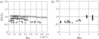
Comparison of the measured frequency of the largest amplitude narrow-band disturbances versus the edge Reynolds number based on the distance from the cone tip (a) and edge Mach number (b) with the data from this work (diamonds), Stetson et al. (Reference Stetson, Thompson, Donaldson and Siler1983) (circles), and Demetriades (Reference Demetriades1977) (squares).

5. Frequency content comparison for high-enthalpy and low-enthalpy conditions
A comparison of the measured frequency (
 $f$
) of the largest amplitude narrow-band disturbances scaled by the edge velocity (
 $U_{E}$
) and the calculated boundary-layer thickness (
 ${\it\delta}$
) versus the edge Reynolds number based on the distance from the cone tip and edge Mach number
 $Ma_{E}$
is presented in figure 10, with the data from this work, Demetriades (Reference Demetriades1977) and Stetson et al. (Reference Stetson, Thompson, Donaldson and Siler1983). The data represent a collection of points over a range of edge Mach number
 $Ma_{E}\approx 4.1{-}7.4$
, edge Reynolds number
 ${\approx}~1{-}4.5\times 10^{6}$
, total enthalpy
 ${\approx}~0.5{-}15~\text{MJ}\,\text{kg}^{-1}$
, wall temperature (
 $T_{W}$
) to reservoir temperature (
 $T_{R}$
) ratio
 $T_{W}/T_{R}\approx 0.05{-}0.8$
, in air, N2 and CO2. It is observed here that
 $2f{\it\delta}/U_{E}$
has a range of 0.6–1.1 for these conditions.
The scatter in the Demetriades (Reference Demetriades1977) and Stetson et al. (Reference Stetson, Thompson, Donaldson and Siler1983) data is smaller than that of the present work; this is to be expected, as the data from the present work is recorded from reflected-shock-tunnel experiments with a short duration and more uncertainty in run conditions than data from Demetriades (Reference Demetriades1977) and Stetson et al. (Reference Stetson, Thompson, Donaldson and Siler1983), which were collected from conventional hypersonic wind-tunnel experiments. In figure 10 there is a weak dependence of peak frequency on edge Reynolds number for all data sets. The systematic differences in
 $2f{\it\delta}/U_{E}$
between data sets are due to the substantial differences between the wall temperature ratio and edge Mach number in the Demetriades (Reference Demetriades1977), Stetson et al. (Reference Stetson, Thompson, Donaldson and Siler1983) and T5 tests. This is consistent with the results of LST (Mack Reference Mack1984), which show that the value of
 $2f{\it\delta}/U_{E}$
for a given geometry is a function of edge Mach number and boundary-layer temperature profile. The weak dependence on Reynolds number is also consistent with LST, which predicts that the second mode of instability is primarily governed by inviscid considerations.
6. Schlieren visualization
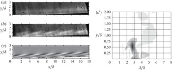
High-speed schlieren cinematography from a conventional
 $z$
-type set-up (Settles Reference Settles2001) is used to record the density disturbances within the boundary layer (figure 11
a–c). The
 $256\times 128$
pixel images were recorded at
 $150$
kframes per second with a Vision Research Phantom v710. The light source is a high-power laser diode (905 nm, PN: 905D3S3J09R), pulsed for 12 ns by a LDP-V 50-100 V3 driver module from Laser Components USA, Inc. The centre of the field of view is downstream of both FLDI detectors, approximately 780 mm from the tip of the cone. Ten frames were selected that bracket a frame in time when an interesting disturbance was observed. An average was constructed of the ten frames (figure 11
a), and 75 % of the average is subtracted from each frame for contrast enhancement. During one of these frames, the instability is captured (figure 11
b).
(a) Schlieren image from N2 shot 2773 (run conditions in table 4). The image is the mean of ten frames. (b) Single image taken from one frame giving a snapshot of the instability
 $(t=1312~{\rm\mu}\text{s})$
, where the time indicates the delay from the pressure rise in the reservoir. (c) Synthetic schlieren image created from the density eigenfunctions as computed by linear-stability theory. The flow is from left to right. The calculated boundary-layer thickness (table 5) and calibration of the image magnification prior to the experiment are used to generate the axis labels. (d) Single-sided spatial Fourier transform of the experimental instability snapshot (b) in the streamwise direction.

Confirmation of the relationship of the observed structures to the density profiles created by the instability was obtained by creating a synthetic schlieren image (figure 11
c) by differentiating the density field shown in figure 1 and representing this as a grey scale image with a threshold simulating the response of the optical system. The synthetic image (figure 11
c) show structures that are similar to the experimental result (figure 11
c). Note that the tilted structures visible in the schlieren images correspond to the density fluctuations shown in figure 1 near the edge of the boundary layer,
 $y\sim {\it\delta}_{.99}$
. An even stronger set of density fluctuations are visible in figure 1 close to the wall,
 $y\sim 0$
, but, due to the limitations of the optical system, the near-wall disturbances cannot be imaged.
The wavelength in the experimental result is determined by a single-sided amplitude spectrum (figure 11
d) of the image brightness in figure 11(b) in the streamwise direction. The most amplified wavelength is
 ${\it\lambda}/{\it\delta}\approx 2.9$
, and occurs at a maximum of approximately 60 % of the boundary-layer thickness. Linear-stability theory calculations (Bitter & Shepherd Reference Bitter and Shepherd2014) indicate a comparable most amplified wavelength of
 ${\it\lambda}/{\it\delta}\approx 3.2$
. The structures of the instability are inclined at an 11–
 $15^{\circ }$
angle to the surface in the experimental result (figure 11
b). This angle is similar to, but smaller than the results reported in Kimmel et al. (Reference Kimmel, Demetriades and Donaldson1996), VanDercreek (Reference VanDercreek2010) and Laurence et al. (Reference Laurence, Wagner, Hannemann, Wartemann, Lüdeke, Tanno and Itoh2012, Reference Laurence, Wagner and Hannemann2014a
,Reference Laurence, Wagner, Ozawa, Schramm and Hannemann
b
). The angle of the structures in the synthetic schlieren image (figure 11
c) are inclined at a 10–
 $13^{\circ }$
angle to the cone surface.
7. Conclusions
The focused laser differential interferometer (FLDI) was used to measure the instability waves prior to transition to turbulent flow at hypervelocity conditions on a slender body in the T5 reflected-shock tunnel. The frequency of the dominant instability observed in this work is in reasonable agreement with previous steady-flow hypersonic wind-tunnel testing in which the second mode was found to dominate transition. Boundary-layer stability analysis was performed and the results show reasonable agreement between the calculated most amplified frequency and measured spectral peaks in the FLDI signals. In addition, comparison of high-speed schlieren visualization with synthetic images derived from linear-stability theory are in good agreement.
We conclude that second-mode instability may be studied at hypervelocity conditions in a reflected-shock tunnel, despite the experimental difficulties. At the outset of this work, it was not clear if unknown ‘bypass’ transition mechanisms would dominate. This would have been a fundamental experimental flaw that would have precluded the examination of instability and transition in a reflected-shock tunnel. Additionally, experiment-to-experiment repeatability concerns were addressed with a facility cleaning regimen. For example, see figure 6(b,c). The edge Reynolds number in the downstream detector of figure 6(b) nearly matches the edge Reynolds number at the upstream detector in figure 6(c); the amplitude of the measured disturbance is also nearly the same, indicating repeatability.
We identify the level of disagreement between the stability analysis and measurements as a topic of future work. Reconciling the predicted and measured frequency content will require considering both the theoretical basis of the computations as well as the sensitivity of the stability-calculation results to the base flow and tunnel conditions. Similar issues have been reported in cold-flow hypersonic facilities where run-condition calculation is less complex and experimental measurement difficulties are more tractable. Researchers are making significant progress in comparing experimental and computational instability growth for cold-flow hypersonics (Marineau et al. Reference Marineau, Moraru, Lewis, Norris, Lafferty and Johnson2015), and we expect those advances to also be of value in hypervelocity flow.
N2 boundary-layer edge conditions.

N2 Boundary-layer instability parameters and scaling.

CO2 boundary-layer edge conditions.

Acknowledgements
The authors thank B. Valiferdowsi and J. Jewell for their assistance in operating and maintaining T5. We are particularly grateful to G. Candler and H. Johnson for generously providing their software and to R. Wagnild for his invaluable help in using these programs. N. Bitter provided key insights into stability theory as well as carried out independent analysis and computations for figures 1 and 11 (the synthetic schlieren images). This work is based in part on the PhD dissertation of the first author Parziale (Reference Parziale2013), and was an activity that was part of National Center for Hypersonic Laminar–Turbulent Research, sponsored by the ‘Integrated Theoretical, Computational, and Experimental Studies for Transition Estimation and Control’ project supported by the US Air Force Office of Scientific Research and the National Aeronautics and Space Administration (FA9552-09-1-0341).
Appendix. Conditions and scaling for N2 and CO2 tests
CO2 boundary-layer instability parameters and scaling.