Implications
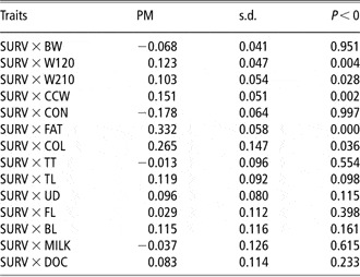
The heritability of longevity, measured as the ability of a cow to reach the next calving is low, although there is some additive genetic variation. As direct selection is difficult due to the delayed availability of phenotypic data, we have estimated the genetic correlation with all available traits in the breeder's association database. No trait was found to be a clear indicator of survival although some traits are positively correlated: fatness (0.33), weight at 120 days (0.12), weight at 210 days (0.10) and cold carcass weight (0.15). Conformation is negatively correlated (−0.18).
Introduction
Longevity or survival are relevant traits in cattle production (Newman et al., Reference Newman, Morris, Baker and Nicoll1992; Melton, Reference Melton1995; Phocas et al., Reference Phocas, Bloch, Chapelle, Bécherel, Renand and Menissier1998). The method of choice for survival analysis has been the proportional hazard model (Cox, Reference Cox1972), which has been adapted to animal breeding (Ducrocq et al., Reference Ducrocq, Quaas, Pollak and Casella1988; Ducrocq and Casella, Reference Ducrocq and Casella1996; De Jong et al., Reference De Jong, Vollema, Van der Beck and Harbers1999) and used to predict breeding values for longevity.
The main difficulty for the practical use of survival traits for selection purposes is the delayed availability of phenotypic data, which may involve an increase in the generation interval (Ducrocq et al., Reference Ducrocq, Quaas, Pollak and Casella1988; Vollema and Groen, Reference Vollema and Groen1997). As a consequence, availability of correlated traits registered early in lifetime can be very helpful. However, the development of a multivariate approach to a continuous survival trait via Markov Chain Monte Carlo methods (Damgaard and Korgsgaard, Reference Damgaard and Korgsgaard2006) is computationally very intensive (González-Recio and Alenda, Reference González-Recio and Alenda2007).
One attractive alternative is to measure survival in discrete-time intervals (e.g. number of calvings in lifetime) as described by Prentice and Gloecker (Reference Prentice and Gloecker1978) and Ducrocq (Reference Ducrocq1999). Within this context, it is possible to analyse longevity records by the use of adapted survival analysis methodologies, such as the sequential threshold model (STM; Albert and Chib, Reference Albert and Chib2001; González-Recio et al., Reference González-Recio, Chang, Gianola and Weigel2005). In addition, González-Recio and Alenda (Reference Kocak, Tekerli, Ozbeyaz and Yuceer2007) have proposed the use of STM for the simultaneous analysis of one discrete-time survival and one Gaussian trait.
The aim of this study is to investigate the genetic correlation of longevity, understood as the cumulated fertility of cows, with growth, carcass, teat and leg morphology, milk production (MILK) and docility (DOC) in the Pirenaica beef cattle breed, by using the STM in bivariate analyses.
Material and methods
Data
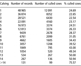
In this study, survival (SURV) was defined as the number of calvings per female, with 15 as the maximum value. The number of available records and the percentage of culled cows in the analysed database provided by the Pirenaica Breeders Association (Confederación Nacional de Asociaciones de Ganado Pirenaico – CONASPI) are shown in Table 1. The database of growth data is made up of 61 833 birth weight (BW) records, 25 812 records of weight at 120 days (W120) and 18 435 records of weight at 210 days (W210). This information was also provided by CONASPI.
Number and percentage of culled cows at each calving

Carcass data were provided by the SIMOGAN database (Sistema de Identificación y Movimiento de Ganado Bovino – National System of Identification and Registration of Cattle Movement) and consist of 29 109 cold carcass weight (CCW) data, 24 912 records for conformation (CON), 22 845 records for fatness (FAT) and 5278 records for meat colour (COL). Carcass CON classes describe the development of carcass profiles, in particular, the essential components of the round, back and shoulder. Under the SEUROP conformation system (CEE no. 2930/81, 1981), six CON classes are defined, represented by the letters S, E, U, R, O and P. The classes correspond to an incremental scale ranging from P, the worst, to S, the best, CON. European regulation allows each country to use three subdivisions of each CON. Thus, the S CON class is subdivided into S+, S, and S−, in declining order. For numerical treatment, the data were transformed into a numerical scale from 1.00 (P) to 6.00 (S) with 16 possible values separated by 0.33. FAT score quantifies the amount of fat on the outside of the carcass and in the thoracic cavity and is defined from 1 (very slim) to 5 (very fat), with increments of 0.25 units. COL was scored from 1 (light) to 7 (dark) following the Beef Colour Standard.
There were 2412 subjective records for teat length (TL), udder depth (UD), forward leg (FL), backward leg (BL), MILK and DOC and 1932 for teat thickness (TT). Subjective traits were scored between 1 (worst) and 9 (best) by expert evaluators from the Pirenaica Breeders Association.
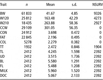
A summary of the phenotypic records is shown in Table 2. The number of individuals with available information for SURV and the Gaussian traits is also presented in Table 2, and it ranges from 0 for traits measured on the slaughterhouse (CCW, CON, FAT, COL) to 9326 with BW. Finally, a pedigree of 205 307 individual-sire-dam entries provided by CONASPI was merged with the phenotypic data.
Summary statistics for the phenotypic data of Gaussian traits and NSURV

BW = birth weight; W120 = weight at 120 days; W210 = weight at 210 days; CCW = cold carcass weight; CON = conformation; FAT = fatness; TT = teat thickness; TL = teat length; UD = udder depth; BL = backward legs; FL = forward legs; MILK = milk production; DOC = docility; NSURV = number of individuals with phenotypic information for longevity.
Statistical model
The STM described by Albert and Chib (Reference Albert and Chib2001) and González-Recio et al. (Reference González-Recio, Chang, Gianola and Weigel2005) was used to analyse SURV as a categorical trait that occurred in sequential order. This means that for an observation to be present at a given stage of the sequence it must have passed through all previous stages. If we suppose that the jth calving is observed for a given cow, the response ti can take the value j only after levels 1, …, j−1 are previously reached, and then either a ‘success’ (survival) or ‘failure’ (culling or death) in level j is observed. Therefore, the probability of survival at calving j, conditional on the fact that the (j−1)th calving has been reached, is given by

where the vector  = (γ 1, γ 2, γ 3, γ 4, …, γj) represents unordered cut-points and
 represents the explanatory effects of the covariates. This probability function is referred to as a discrete-time hazard function (Prentice and Gloecker, Reference Prentice and Gloecker1978; Tutz, Reference Tutz1990 and Reference Tutz1991). Therefore, a single latent variable can be used to represent the cow's propensity to pass from one category to the next (González-Recio and Alenda, Reference González-Recio and Alenda2007). Corresponding to the jth calving and defining latent variables (ωij), we observe ti = 1 if ωi 1 ⩽ γ 1, and ti = 2 if the first latent variable is ωi 1 > γ 1 and the second latent variable is ωi 2 ⩽ γ 2.
In general,

In association with the latent variable vector ( ), we implemented a Bayesian bivariate model to analyse the genetic correlation for discrete-time survival (SURV), jointly with Gaussian traits (BW, W120, W210, CCW, CON, FAT, COL, MILK, DOC, UD, TT, TL, FL and BL). The latent variable representation can be simplified by incorporating the cut-points (γi) into the mean function and fixing one of the cut-points; usuallyγ 1 = 0.
Gaussian–STM model
A bivariate model was defined for the latent variable ( ) for SURV and y for the Gaussian traits. The model assumed for the latent variable was a repeatability model:

for each of the Gaussian traits (y), the model was

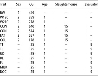
where bω and bg are the vectors of systematic effects for SURV and each Gaussian trait, respectively. For SURV, systematic effects consist of cut-points ( ) associated with order of parity (15 levels), calving ease (2 levels – no help and help), sex of calf (male or female), season of parity (summer, fall, winter and spring), year (51 levels) and farm (1964 levels). For Gaussian traits, systematic effects and number of levels included in the model are given in Table 3. Furthermore, uω and ug are the vectors of additive genetic effects for SURV and each Gaussian trait; pω is the permanent environment effect for the SURV trait and eω and eg are the vector of residual effects for SURV and each of Gaussian traits, respectively. Finally, Pω , Xω, Xg, Zω, Zg and Wω are known incidence matrices corresponding to cut-points, systematic, genetic and permanent environment effects.
Number of levels in the systematic effects for Gaussian traits

CG = contemporary groups; BW = birth weight; W120 = weight at 120 days; W210 = weight at 210 days; CCW = cold carcass weight; CON = conformation; FAT = fatness; TT = teat thickness; TL = teat length; UD = udder depth; BL = backward legs; FL = forward legs; MILK = milk production; DOC = docility.
Gibbs sampler
Posterior distributions of all the parameters in the model were estimated using a single parameter update Gibbs sampling algorithm (Gelfand and Smith, Reference Gelfand and Smith1990) with a data augmentation step (Tanner and Wong, Reference Tanner and Wong1987; Sorensen et al., Reference Sorensen, Andersen, Gianola and Korsgaard1995) using software developed by the authors. The joint posterior distribution of all unknowns in the model was

where p(t|γ) is defined as in expression (1). Further,

where

where  is the (co)variance matrix for the additive genetic effect, and A is the numerator relationship matrix.
The prior distribution for the permanent environment effects was

Prior distributions for variance components (G,  and
 ) and the systematic effects (bg, bω) and cut-points (
 ) were assumed uniform.
From that, the Gibbs sampling procedure develops an iterative sampling scheme from the full conditional distributions. First, the latent variables ( ) were augmented from the following truncated Gaussian distributions:

or

where ωik is the kth latent variable for the ith data, Φ( ) and φ( ) are the Gaussian distribution and function densities, and pik, xik, zik and wik are the corresponding rows of the incidence matrices.
Given the augmented latent variable (ω), the Gibbs sampler algorithm is equivalent to a standard multiple trait animal model analysis (Van Tassell and Van Vleck, Reference Van Tassell and Van Vleck1996). Thus, the posterior conditional distributions for systematic effects, breeding values and permanent environmental effects were univariate Gaussian, the posterior conditional distribution for G was an inverse Wishart and the posterior conditional distributions for  and
 were inverse χ 2.
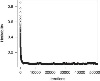
The analyses were run as a single chain of 525 000 cycles and the first 25 000 were discarded. Convergence was checked by the visual inspection of the chains and with the procedure of Raftery and Lewis (Reference Raftery and Lewis1992). An example of convergence is presented in Figure 1. All samples were stored for computing posterior means, medians, modes, s.d. and credible regions.
Convergence plot of the heritability for survival.

Results and discussion
SURV
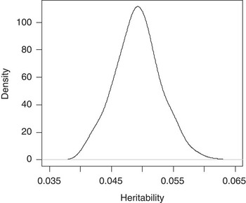
The posterior mean heritability of SURV, measured as the liability to reach the following parity was 0.05, substantially lower than the results presented by González-Recio and Alenda (Reference Kocak, Tekerli, Ozbeyaz and Yuceer2007) and Van Melis et al. (Reference Van Melis, Oliveira, Eler, Ferraz, Casellas and Varona2010) using the same statistical approach as Holstein and Nellore, respectively. Moreover, the figure is within the range of results reported by Forabosco et al. (Reference Forabosco, Bozzi, Filippini, Boettcher, Van Arendonk and Bijma2006) and Zavadilova et al. (Reference Zavadilova, Sitpkova, Nemcova, Bouska and Matejickova2009) in Chianina and Fleckvieh or Simmental, using linear models and survival analysis. However, the posterior distribution of heritability (Figure 2) ranged between 0.04 and 0.06, indicating that there is some additive genetic variation for SURV, so selection for the trait is still feasible, although the expected genetic response is very low.
Posterior distribution of heritability for survival on the underlying scale.

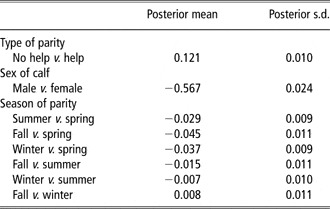
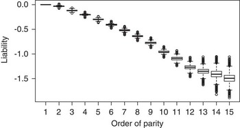
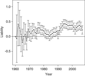
The results for the posterior mean estimates of the systematic effects for survival shown in Table 4 indicate that ability to reach the following calving is reduced when the cow has a male calf and when some kind of veterinary assistance is required in calving, confirming the results of Kocak et al. (Reference Kocak, Tekerli, Ozbeyaz and Yuceer2007) and Szabo and Dakay (Reference Szabo and Dakay2009). A relevant effect was also found regarding the season of parity, a higher ability to survive was detected for cows that calve in spring, as reported previously by Szabo and Dakay (Reference Szabo and Dakay2009). In addition, and as illustrated in Figure 3, SURV is reduced in older cows. The results of the year effect are presented in Figure 4 and indicate that SURV is slightly greater in recent years (1990 to 2008). This last result can be probably attributed to the improvement of the recording system in the last two decades. Finally, the herd effect was very heterogeneous, with an average very close to zero and a standard deviation of posterior estimates of 0.36.
Posterior mean and standard deviations of systematic effects for survival

Boxplot for the posterior distributions of the effect order of parity for the liability of survival.

Evolution of year effect for the liability of survival.

Heritabilities for Gaussian traits
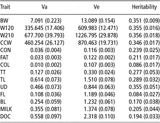
The posterior mean (and standard deviance) estimates for variance components and heritabilities for growth, carcass, morphological and DOC traits from the bivariate analysis are presented in Table 5. The posterior estimates of the additive genetic variance indicate that a relevant additive genetic variance exists in all of them. In particular, the posterior mean estimates of heritability for growth traits is approximately 0.35, similar to the estimates obtained previously in the same population (Altarriba et al., Reference Altarriba, Yagüe, Moreno and Varona2009) and within the range of previous estimates in other beef cattle breeds (Koots et al., Reference Koots, Gibson, Smith and Wilton1994; Rios-Utrera and Van Vleck, Reference Rios-Utrera and Van Vleck2004).
Posterior means and standard deviations (in brackets) for Va and Ve and heritability coefficients

Va = additive variances; Ve = residual variances; BW = birth weight; W120 = weight at 120 days; W210 = weight at 210 days; CCW = cold carcass weight; CON = conformation; FAT = fatness; TT = teat thickness; TL = teat length; UD = udder depth; BL = backward legs; FL = forward legs; MILK = milk production; DOC = docility.
The posterior estimates for the heritability of CON and FAT were 0.24 and 0.21, coherent, but slightly lower than the estimates reported in previous studies in Nellore (Van Melis et al., Reference Van Melis, Eler, Silva and Ferraz2003) and Angus (Cardoso et al., Reference Cardoso, Cardellino and Campos2004). In addition, for COL, our posterior estimate was 0.09, lower than the estimate obtained in the same population (Altarriba et al., Reference Altarriba, Yagüe, Moreno and Varona2009) in a previous study and in other populations (Shojo et al., Reference Shojo, Okanishi, Anada, Oyama and Mukai2006).
Posterior mean estimates of heritability of teat morphology traits (TT, TL and UD) ranged between 0.28 and 0.36, slightly higher than the results obtained by Zavadilova et al. (Reference Zavadilova, Sitpkova, Nemcova, Bouska and Matejickova2009), and similar to Vollema and Groen (Reference Vollema and Groen1997) and Vukasinovic et al. (Reference Vukasinovic, Schleppi and Kunzi2002) in dairy cattle. The posterior mean estimates for heritability of leg CON were lower, 0.08 for FL and 0.17 for BL, but within the range of those obtained by DeGroot et al. (Reference DeGroot, Keown, Van Vleck and Marotz2002), Wiggans et al. (Reference Wiggans, Thornton, Neitzel and Gengler2006) and Mantovani et al. (Reference Mantovani, Cassandro, Contiero, Albera and Bittante2010) in Holstein, Brown Swiss and Piemontese breeds, respectively.
The posterior mean estimate for heritability of MILK, measured subjectively, was 0.21, lower than the estimates of Phocas and Sapa (Reference Phocas and Sapa2004) in Charolais, Limousin and Blonde d'Aquinaine and slightly lower than the estimates in dairy cattle. Finally, the posterior mean estimate of the heritability of DOC was 0.19, confirming the evidence of additive genetic variance for this trait, as suggested by the studies of Le Neindre et al. (Reference Le Neindre, Trillat, Sapa, Menissier, Bonnet and Chupin1995) and Phocas et al. (Reference Phocas, Boivin, Sapa, Trillat, Boissy and Le Neindre2006) in Limousin cattle.
Genetic correlations
The posterior mean and standard deviation estimates for genetic correlations with survival are shown in Table 6. The posterior probability below zero is also displayed. The results indicate a positive correlation of survival with W120, W210, CCW and FAT and negative correlation with CON. A positive genetic correlation with weight has previously been suggested by several authors (Rogers et al., Reference Rogers, Gaskins, Johnson and MacNeil2004; Tarres et al., Reference Tarres, Puig, Ducrocq and Piedrafita2004; Zavadilova et al., Reference Zavadilova, Sitpkova, Nemcova, Bouska and Matejickova2009; Van Melis et al., Reference Van Melis, Oliveira, Eler, Ferraz, Casellas and Varona2010). However, there was almost no correlation with BW; this was probably caused by the positive correlation between dam and calf BW and by the association of these traits with calving difficulty, as noted previously. The null genetic correlation could be composed of a positive relation with weight and a negative relation with calving difficulty. The other trait positively correlated with SURV is FAT: cows with greater ability to accumulate fat are more able to survive to the next parity.
PM, s.d. and posterior probability below zero (P < 0) for the genetic correlation between SURV and Gaussian traits

PM = posterior means; SURV = survival; BW = birth weight; W120 = weight at 120 days; W210 = weight at 210 days; CCW = cold carcass weight; CON = conformation; FAT = fatness; TT = teat thickness; TL = teat length; UD = udder depth; FL = forward legs; BL = backward legs; MILK = milk production; DOC = docility.
The only trait that clearly indicates a negative correlation with SURV was CON, surely due to a higher probability of presenting calving difficulties during productive life for the individuals with higher muscularity. This result contrasts with results obtained by Forabosco et al. (Reference Forabosco, Groen, Bozzi, Van Arendonk, Filippini, Boettcher and Bijma2004) in the Chianina breed, although it must be recognised that the Chianina breed has a higher muscularity development that implies regular assisted calving, which is considered as natural by the farmer. In contrast, most calvings are unassisted (more than 95%) in the Pirenaica breed.
The posterior distribution of the genetic correlation between morphology, DOC and milk traits with SURV do not indicate a clear correlation, although the amount of available data is reduced when compared with weight, FAT and muscularity traits. However, a tendency to a positive correlation with COL, TL, UD, BL and DOC was observed and this should be confirmed with future research on a larger dataset. Nevertheless, it must be remarked that the posterior probability is lower than 0.01 than a genetic correlation with SURV over 0.5 for each of the analysed traits. Thus, given the available information, it is clear that none of the analysed traits can be used as an efficient early predictor of survival in the Pirenaica beef cattle breed.
Acknowledgements
The authors would like to thank the Pirenaica Breeders Association (Confederación Nacional de Asociaciones de Ganado Pirenaico) and the Spanish Ministry of Agriculture (Sistema de Identificación y Movimiento de Ganado Bovino database) for the provision of data used in this work. Financial support was provided by Grants AGL2007-66147 and AGL2010-15903.