1 Introduction
High angle-of-attack (AoA) flows with vortex shedding are found in applications of insect wings (Ellington et al. Reference Ellington, Van Den Berg, Willmott and Thomas1996; Muijres et al. Reference Muijres, Johansson, Barfield, Wolf, Spedding and Hedenstrom2008; Bomphrey, Taylor & Thomas Reference Bomphrey, Taylor and Thomas2009), micro air vehicles (Dickinson & Gotz Reference Dickinson and Gotz1993), fixed delta wings (Polhamus Reference Polhamus1971) and turbines undergoing pitching, plunging, heaving or a combination of these (Choudhry et al. Reference Choudhry, Leknys, Arjomandi and Kelso2014). The role of free vortices on the unsteady lift is of primary importance and is believed to be responsible for lift enhancement, dynamic stall and wake capture. After Dickinson & Gotz (Reference Dickinson and Gotz1993), who attributed lift enhancement to the production and attachment of a leading-edge vortex (LEV) in analogy to the mechanism of force production in delta-wing aircraft (Polhamus Reference Polhamus1971), LEV was believed to be one of the major lift production mechanisms for insect flight problems (Ellington et al. Reference Ellington, Van Den Berg, Willmott and Thomas1996; Bomphrey et al. Reference Bomphrey, Lawson, Harding, Taylor and Thomas2005, Reference Bomphrey, Taylor and Thomas2009; Muijres et al. Reference Muijres, Johansson, Barfield, Wolf, Spedding and Hedenstrom2008).
Free vortices may be treated as vortex sheet discontinuities (Wagner Reference Wagner1925; Graham Reference Graham1983; Jones Reference Jones2003; Pullin & Wang Reference Pullin and Wang2004), concentrated point vortices with a region of vortices represented by a single point vortex (Graham Reference Graham1983; Pullin & Wang Reference Pullin and Wang2004; Wang & Eldredge Reference Wang and Eldredge2013; Hemati, Eldredge & Speyer Reference Hemati, Eldredge and Speyer2014), discrete point vortices as used in discrete vortex simulation (Clement Reference Clement1973; Ansari, Zbikowski & Knowles Reference Ansari, Zbikowski and Knowles2006; Xia & Mohseni Reference Xia and Mohseni2013) or continuously distributed vortices as given by computational fluid dynamics (CFD) studies (Wang Reference Wang2000; Knowles et al. Reference Knowles, Wilkins, Ansari and Zbikowski2007; Li & Lu Reference Li and Lu2012). The force may be related to free vortices through the use of various equivalent forms of the moment equation for flow, such as the algebraic Bernoulli equation (Xia & Mohseni Reference Xia and Mohseni2013), the unsteady Blasius equation (Milne-Thomson Reference Milne-Thomson1960; Streitlien & Triantafyllou Reference Streitlien and Triantafyllou1995; Pitt Ford & Babinsky Reference Pitt Ford and Babinsky2013) and integral approaches (Wu Reference Wu1981; Saffman Reference Saffman1992; Howe Reference Howe1995; Wu, Lu & Zhuang Reference Wu, Lu and Zhuang2007).
Among these approaches, the vortex sheet and concentrated vortex representations are more suitable for analytical solution. For instance, the singular behaviour of the initial lift due to rolling of the trailing-edge vortex sheet at high AoA was predicted analytically by Graham (Reference Graham1983). For an accelerating plate, the evolution of vortex sheet spirals from both leading and trailing edges and normal force were solved by Jones (Reference Jones2003) for all time using a boundary integral approach and Pullin & Wang (Reference Pullin and Wang2004) for short time using a similarity expansion of the Birkhoff–Rott equation. Li & Wu (Reference Li and Wu2015) used a hybrid vortex sheet point vortex approach, with the sheet effect treated analytically while the additional vortices, not representable by a planar sheet, are treated numerically. Quite recently, Darakananda et al. (Reference Darakananda, Eldredge, Colonius and Williams2016) also developed a hybrid vortex sheet point vortex approach, in which the vortex sheet’s spiral cores are represented by point vortices.
Despite the various achievements of past studies, part of which were reviewed by Wang (Reference Wang2005) and Choudhry et al. (Reference Choudhry, Leknys, Arjomandi and Kelso2014), it is still desirable to have a more physical picture of the effect of vortices on force behaviour (Xia & Mohseni Reference Xia and Mohseni2013). For this purpose, Li & Wu (Reference Li and Wu2015) considered low enough AoAs (up to
 $20^{\circ }$
) and generated a vortex force line map which can be used to explicitly indicate the lift-enhancing and -reducing directions, interpret the effect of the sign and position of vortices on the lift, and identify the origins of lift oscillations and peaks. Li, Bai & Wu (Reference Li, Bai and Wu2015a
,Reference Li, Bai and Wu
b
) verified numerically that this approach seems to work also for high AoAs, though a theoretical study for high AoAs is lacking.
One purpose in this work is thus to generalize and validate the vortex force approach and vortex force map of Li & Wu (Reference Li and Wu2015) to high AoA flows. The derivation of the vortex force method for high AoAs is presented in § 2, where we also outline the discrete vortex simulation and CFD approaches used in this paper. For high AoA, vortex shedding is intensive, so that circulation production would be important; thus the extension will includes a rigorous consideration of this. The impulsively starting flow of a flat plate is used for validation and application.
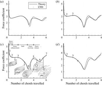
The graphic display of the force effect by each individual vortex and the vortex force line map for high AoA will be considered in § 3.1. Since LEVs and trailing-edge vortices (TEVs) are observable on experimental pictures and in graphic displays of CFD results, and since their trajectories can be easily followed, we study in § 3.2 the possibility to apply the vortex force map to these concentrated vortices and to identify critical regions for force production or enhancement by LEVs and TEVs. The resulting approaches will then be used in § 3.3 to associate various stages of the force curve to the positions of LEVs and TEVs. By this study we find that the force curve can be more physically decomposed into four repeatable stages, which are force release, force enhancement, stall and force recovery.
To see how a vortex affects the force more clearly, a pressure distribution analysis is used in § 3.4 to relate the various force stages and critical regions to the inducing effect of an LEV and a TEV. Possible correction by viscous effects will be considered in § 3.5.
The present study is expected to offer more knowledge about force variation in large AoA flows, as will be summarized in § 4.
2 An inviscid force method for high AoA and its validation
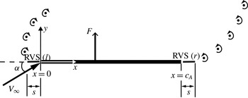
As displayed in figure 1, we use a body-fixed frame so that the inflow has a speed
 $V_{\infty }$
at an AoA
 ${\it\alpha}$
. For the present problem with a flat plate, the force is normal to the plate due to leading-edge separation (Pullin & Wang Reference Pullin and Wang2004). To show the new ingredients of the present extension, we first recall the related modelling from the previous study.
Vortex flow around a flat plate at high AoA.

2.1 The modelling from the previous study
The study by Li & Wu (Reference Li and Wu2015) is essentially concerned with an amended Wagner lift model, which includes the influence of additional vortices that are not included in the planar trailing-edge vortex sheet. An analytical lift is derived which explicitly shows the effect of additional vortices on the Wagner lift (Wagner Reference Wagner1925). The conclusion for an AoA up to
 $20^{\circ }$
is that LEVs close to the leading edge elevate the Wagner lift curve, while a strong LEV convected to the trailing edge is detrimental to lift production by inducing a strong TEV moving in the lift-reducing direction.
Apart from the amended Wagner lift model, Li & Wu (Reference Li and Wu2015) also gave a total vortex force model in which the lift is expressed as a function of the velocity of point vortices. However, the total vortex force model has been obtained by using the thin airfoil assumption and by simply dropping out, without justification, some terms due to vortex sheets in the amended Wagner model. For high AoA, the thin airfoil assumption does not hold. Moreover, the total vortex force approach has been obtained by dropping out those terms that are not directly related to discrete vortices. Also, the importance of circulation production forces is not covered seriously in previous works.
In the following, we perform a rigorous derivation for normal force at high AoA. Apart from dropping the thin airfoil assumption, a residual vortex sheet at both leading and trailing edges is included in the vortex system and the importance of circulation production, omitted in the previous study, is discussed here. Despite these new ingredients, the derivation has a number of steps similar to the work of Li & Wu (Reference Li and Wu2015). For completeness, we still give enough detail in the derivation.
2.2 Vortex representation and force in its primitive form
Consider some instant
 $t=t_{n}$
at which all free vortices are represented by point vortices, the number
 $I$
of which is arbitrary. For point vortex
 $i$
, with
 $i=1,2,\ldots ,I$
, the circulation is
 ${\it\Gamma}_{i}$
(positive if it is anticlockwise), the position is
 $(x_{i},y_{i})$
and the velocity is
 $\boldsymbol{U}_{i}=(u_{i},v_{i})=({\dot{x}}_{i},{\dot{y}}_{i})$
. Following the vortex shedding picture discussed by Graham (Reference Graham1980), a residual vortex sheet, representing vortices being shed yet not represented by point vortices, is assumed at both leading and trailing edges. See figure 1 for a schematic display of the vortex system. These residual vortex sheets are assumed to be of vanishing and equal length
 $S$
; once these vortex sheets are large, they are represented by new point vortices. Representing a residual vortex sheet in this way allows for capturing of the effect of circulation production.
Let
 $k_{r}(s,t)$
be the circulation per unit length of the residual vortex sheet from the trailing edge, where
 $s$
with
 $0<s<S$
is the local coordinate (positive in the rightward direction). Let
 $k_{l}(s,t)$
be the circulation per unit length of the residual vortex sheet from the leading edge, where
 $s$
with
 $0<s<S$
is the local coordinate (positive in the leftward direction). Using the coordinate
 $s$
in this way and assuming the residual vortex sheets to have equal length will cause the force term to contain
 $k_{l}$
and
 $k_{r}$
in combination
 $k=k_{l}+k_{r}$
. We use an overdot to denote the time derivative; for instance,
 $\dot{{\it\Gamma}}_{i}=\text{d}{\it\Gamma}_{i}/\text{d}t$
.
Let
 ${\it\gamma}(x,t)$
be the circulation per unit length of bound vortices. The bound circulation
 ${\it\Gamma}_{b}$
and bound vorticity moment
 ${\it\Theta}_{b}$
are defined as
 $$\begin{eqnarray}{\it\Gamma}_{b}=\int _{0}^{c_{A}}{\it\gamma}(x,t)\,\text{d}x,\quad {\it\Theta}_{b}=\int _{0}^{c_{A}}{\it\gamma}(x,t)x\,\text{d}x.\end{eqnarray}$$
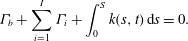
The Kelvin condition for conservation of total circulation gives
 $$\begin{eqnarray}{\it\Gamma}_{b}+\mathop{\sum }_{i=1}^{I}{\it\Gamma}_{i}+\int _{0}^{S}k(s,t)\,\text{d}s=0.\end{eqnarray}$$
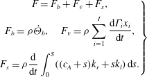
With the present vortex representation, the normal force is given by
 $$\begin{eqnarray}\left.\begin{array}{@{}c@{}}F=F_{b}+F_{v}+F_{s},\\ F_{b}={\it\rho}\dot{{\it\Theta}}_{b},\quad F_{v}={\it\rho}\displaystyle \mathop{\sum }_{i=1}^{I}\frac{\text{d}{\it\Gamma}_{i}x_{i}}{\text{d}t},\\ F_{s}={\it\rho}\displaystyle \frac{\text{d}}{\text{d}t}\displaystyle \int _{0}^{S}((c_{A}+s)k_{r}+sk_{l})\,\text{d}s.\end{array}\right\}\end{eqnarray}$$
This force formula may follow from various force theories, such as the integral vortex moment approach (Wu Reference Wu1981), impulse approach (Saffman Reference Saffman1992) and integral equivalent of point vortex force approaches; see Li et al. (Reference Li, Bai and Wu2015a
) for a discussion. Here,
 $F_{b},~F_{v}$
and
 $F_{s}$
are due to bound vortices, (free) point vortices and residual vortex sheets, respectively. Since
 ${\it\gamma}$
is a combination effect of the geometry and the images of free vortices, the bound vortex moment
 ${\it\Theta}_{b}$
can also be decomposed into
 ${\it\Theta}_{b}={\it\Theta}_{b}^{(g)}+{\it\Theta}_{b}^{(PV)}+{\it\Theta}_{b}^{(RVS)}$
, where the superscript
 $g$
refers to influence from geometry (shape of airfoil and angle of attack),
 $\text{PV}$
refers to influence from point vortices and
 $\text{RVS}$
refers to influence from residual vortex sheets (the bound circulation
 ${\it\Gamma}_{b}$
can be decomposed similarly). Since the plate is considered fixed once started, we have
 $\dot{{\it\Theta}}_{b}^{(g)}=0$
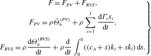
. Thus, (2.3) can be rewritten as
 $$\begin{eqnarray}\left.\begin{array}{@{}c@{}}F=F_{PV}+F_{RVS},\\ F_{PV}={\it\rho}\dot{{\it\Theta}}_{b}^{(PV)}+{\it\rho}\displaystyle \mathop{\sum }_{i=1}^{I}\frac{\text{d}{\it\Gamma}_{i}x_{i}}{\text{d}t},\\ F_{RVS}={\it\rho}\displaystyle \frac{\text{d}{\it\Theta}_{b}^{(RVS)}}{\text{d}t}+{\it\rho}\frac{\text{d}}{\text{d}t}\int _{0}^{S}((c_{A}+s)k_{r}+sk_{l})\,\text{d}s.\end{array}\right\}\end{eqnarray}$$
2.3 Circulations, vorticity moment and force expressions
To get the force from (2.4), we need explicit expressions of
 ${\it\Theta}_{b}$
(and thus
 ${\it\gamma}(x,t)$
) and
 $k$
. The intensities
 ${\it\gamma}(x,t)$
and
 $k(s,t)$
are now determined from boundary condition
 $v(x,0)=-V_{\infty }\sin {\it\alpha}$
and Kelvin condition (2.2). Here,
 $v(x,0)$
is the normal velocity component induced by all vortices. When the Biot–Savart relation is used for
 $v(x,0)$
, we get from the boundary condition the following expression for
 ${\it\gamma}({\it\xi})$
:
 $$\begin{eqnarray}\frac{1}{2{\rm\pi}}\int _{0}^{c_{A}}\frac{{\it\gamma}({\it\xi})}{x-{\it\xi}}\,\text{d}{\it\xi}=v^{(g)}+v^{(PV)}+v^{(RVS)}.\end{eqnarray}$$
Here we have
 $v^{(g)}=-V_{\infty }\sin {\it\alpha}$
,
 $v^{(PV)}=\sum _{i=1}^{I}({\it\Gamma}_{i}/2{\rm\pi})(x_{i}-x)/((x-x_{i})^{2}+y_{i}^{2})$
and
 $v^{(RVS)}=-(1/2{\rm\pi})\int _{0}^{S}k_{r}(s)\,\text{d}s/(x-c_{A}-s)-(1/2{\rm\pi})\int _{0}^{S}k_{l}(s)\,\text{d}s/(x+s)$
, which represent the contributions from geometry, point vortices and residual vortex sheets, respectively. Equation (2.5) can be solved by setting
 $$\begin{eqnarray}{\it\gamma}({\it\theta})=2V_{\infty }A_{0}\frac{1+\cos {\it\theta}}{\sin {\it\theta}}+2V_{\infty }\mathop{\sum }_{n=0}^{n=\infty }A_{n}\sin (n{\it\theta}),\end{eqnarray}$$
where
 ${\it\theta}$
with
 $0<{\it\theta}<{\rm\pi}$
is related to
 $x$
through
 $x=(1/2)c_{A}(1-\cos {\it\theta})$
. Putting (2.6) into (2.5) gives a set of equations for
 $A_{n}$
which can be solved using the standard method (Anderson Reference Anderson2007). With
 $A_{n}$
and then
 ${\it\gamma}$
thus obtained, the circulation
 ${\it\Gamma}_{b}(t)$
and moment
 ${\it\Theta}_{b}(t)$
defined by (2.1) can be straightforwardly calculated. This calculation is similar to Li & Wu (Reference Li and Wu2015) so we omit the details. The results are
 $$\begin{eqnarray}{\it\Gamma}_{b}^{(g)}=-{\rm\pi}c_{A}V_{\infty }\sin {\it\alpha},\quad {\it\Gamma}_{b}^{(PV)}=\mathop{\sum }_{i=1}^{I}C_{i}{\it\Gamma}_{i},\quad {\it\Gamma}_{b}^{(RVS)}=-{\it\Gamma}_{m}-\int _{0}^{S}k\,\text{d}s\end{eqnarray}$$
and
 $$\begin{eqnarray}\left.\begin{array}{@{}c@{}}{\it\Theta}_{b}^{(g)}=\displaystyle \frac{c_{A}}{4}{\it\Gamma}_{b}^{(g)},\quad {\it\Theta}_{b}^{(PV)}=c_{A}\displaystyle \mathop{\sum }_{i=1}^{I}E_{i}{\it\Gamma}_{i},\\ {\it\Theta}_{b}^{(RVS)}=\displaystyle -\int _{0}^{S}sk\,\text{d}s-\int _{0}^{S}c_{A}k_{r}\,\text{d}s+{\it\Upsilon}-\frac{c_{A}}{2}{\it\Gamma}_{m}.\end{array}\right\}\end{eqnarray}$$
Here,
 ${\it\Gamma}_{m}$
and
 ${\it\Upsilon}$
are integral functions of
 $k=k_{l}(s,t)+k_{r}(s,t)$
defined by
 $$\begin{eqnarray}{\it\Gamma}_{m}=-\int _{0}^{S}\frac{\sqrt{c_{A}+s}}{\sqrt{s}}k(s,t)\,\text{d}s,\quad {\it\Upsilon}=\int _{0}^{S}\sqrt{s(c_{A}+s)}k(s,t)\,\text{d}s.\end{eqnarray}$$
The parameters
 $C_{i}=C(p_{i},q_{i})$
and
 $E_{i}=E(p_{i},q_{i})$
are functions of non-dimensional position
 $$\begin{eqnarray}(p,q)=\left(\frac{2}{c_{A}}\left(x-\frac{1}{2}c_{A}\right),\frac{2}{c_{A}}y\right)\end{eqnarray}$$
for vortex
 $i$
; the explicit expressions are
 $$\begin{eqnarray}\left.\begin{array}{@{}c@{}}C(p_{i},q_{i})=\displaystyle \frac{1}{{\rm\pi}}\left(p_{i}({\it\lambda}_{i}^{(0)}-{\it\lambda}_{i}^{(1)})+{\it\lambda}_{i}^{(1)}-\frac{{\it\lambda}_{i}^{(0)}+{\it\lambda}_{i}^{(2)}}{2}\right),\\ E(p_{i},q_{i})=\displaystyle \frac{1}{4{\rm\pi}}\left((p_{i}-1)({\it\lambda}_{i}^{(0)}+{\it\lambda}_{i}^{(2)})+\left(\frac{3}{2}-2p_{i}\right){\it\lambda}_{i}^{(1)}+\frac{1}{2}{\it\lambda}_{i}^{(3)}\right),\\ {\it\lambda}_{i}^{(n)}=\displaystyle \int _{0}^{{\rm\pi}}\frac{\cos (n{\it\beta})}{(p_{i}+\cos {\it\beta})^{2}+q_{i}^{2}}\,\text{d}{\it\beta},\quad n\geqslant 0.\end{array}\right\}\end{eqnarray}$$
Putting (2.8) for
 ${\it\Theta}_{b}^{(PV)}$
and
 ${\it\Theta}_{b}^{(RVS)}$
into (2.4), we get
 $F_{PV}=F_{PV}^{(vm)}+F_{PV}^{(cp)}$
, where
 $$\begin{eqnarray}F_{PV}^{(vm)}={\it\rho}\mathop{\sum }_{i=1}^{I}(u_{i}+c_{A}{\dot{E}}_{i}){\it\Gamma}_{i},\quad F_{PV}^{(cp)}={\it\rho}\mathop{\sum }_{i=1}^{I}(x_{i}+c_{A}E_{i})\dot{{\it\Gamma}}_{i},\end{eqnarray}$$
and
 $F_{RVS}=-(1/2)c_{A}{\it\rho}\dot{{\it\Gamma}}_{m}+{\it\rho}\dot{{\it\Upsilon}}$
(the terms due to
 $k_{l}(s,t)$
and
 $k_{r}(s,t)$
happen to disappear by mutual cancellation). In appendix A, we will show that
 $\dot{{\it\Upsilon}}=0$
for
 $S\rightarrow 0$
. Thus
 $$\begin{eqnarray}F_{RVS}=-\frac{c_{A}}{2}{\it\rho}\dot{{\it\Gamma}}_{m}.\end{eqnarray}$$
The function
 ${\it\Gamma}_{m}$
is defined by (2.9a,b
). Inserting the bound circulation
 ${\it\Gamma}_{b}$
, with its three components defined by (2.7), into the Kelvin condition (2.2) gives an explicit expression for
 $\dot{{\it\Gamma}}_{m}$
:
 $$\begin{eqnarray}\dot{{\it\Gamma}}_{m}=\frac{\text{d}}{\text{d}t}\mathop{\sum }_{i=1}^{I}(1+C_{i}){\it\Gamma}_{i}.\end{eqnarray}$$
Thus, the force (2.13) reduces to
 $F_{RVS}=-(1/2){\it\rho}c_{A}\,\text{d}{\it\Gamma}_{m}/\text{d}t$
or
 $F_{RVS}=F_{RVS}^{(vm)}+F_{RVS}^{(cp)}$
, with
 $$\begin{eqnarray}F_{RVS}^{(vm)}=-\frac{1}{2}{\it\rho}c_{A}\mathop{\sum }_{i=1}^{I}{\dot{C}}_{i}{\it\Gamma}_{i},\quad F_{RVS}^{(cp)}=-\frac{1}{2}{\it\rho}c_{A}\mathop{\sum }_{i=1}^{I}(1+C_{i})\dot{{\it\Gamma}}_{i}.\end{eqnarray}$$
The total force can therefore be decomposed as
 $F=F^{(vm)}+F^{(cp)}$
, with
 $F^{(vm)}=F_{PV}^{(vm)}+F_{RVS}^{(vm)}$
and
 $F^{(cp)}=F_{PV}^{(cp)}+F_{RVS}^{(cp)}$
. When (2.11) and (2.14) are used, we get
 $$\begin{eqnarray}\displaystyle & \displaystyle F^{(vm)}={\it\rho}\mathop{\sum }_{i=1}^{I}\left(u_{i}+c_{A}{\dot{E}}_{i}-\frac{1}{2}c_{A}{\dot{C}}_{i}\right){\it\Gamma}_{i}, & \displaystyle\end{eqnarray}$$
 $$\begin{eqnarray}\displaystyle & \displaystyle F^{(cp)}={\it\rho}\mathop{\sum }_{i=1}^{I}\left(x_{i}+c_{A}E_{i}-\frac{1}{2}c_{A}(1+C_{i})\right)\dot{{\it\Gamma}}_{i}. & \displaystyle\end{eqnarray}$$
2.4 Circulation production force
Once the point vortex
 $i$
is released, its circulation does not vary in time due to the Kelvin theorem, that is,
 $\dot{{\it\Gamma}}_{i}=0$
. Thus,
 $F^{(cp)}$
defined by (2.17) should vanish once the sum is defined over all point vortices already released. However, in deriving the force formula, we have assumed a vanishing size for residual vortex sheets. In a discrete vortex simulation, the time step may sometimes not be small enough, so that the residual vortex sheets considered here do not represent the whole residual vortices shedding during a given time step. In order to increase the accuracy, as will be checked in § 2.6, we use
 ${\it\Gamma}_{LE}$
and
 ${\it\Gamma}_{TE}$
to represent the whole residual vortices. With
 $\dot{{\it\Gamma}}_{LE}\neq 0$
and
 $\dot{{\it\Gamma}}_{TE}\neq 0$
and with
 $\dot{{\it\Gamma}}_{i}=0$
for point vortices already released, the use of (2.17) gives
 $$\begin{eqnarray}F^{(cp)}={\textstyle \frac{1}{2}}{\it\rho}c_{A}(R_{LE}\dot{{\it\Gamma}}_{LE}+R_{TE}\dot{{\it\Gamma}}_{TE}),\end{eqnarray}$$
where
 $R_{LE}=R(p_{LE},q_{LE})$
and
 $R_{TE}=R(p_{TE},q_{TE})$
, with
 $R(p,q)=p+2E(p,q)-C(p,q)$
.
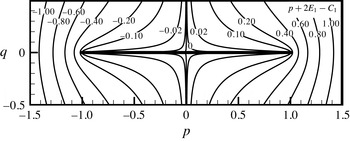
Since
 $F^{(cp)}$
is due to the production of residual vortices during a discrete time step, it is a discrete circulation production force. Figure 2 displays the factor
 $R(p,q)$
in the two-dimensional space
 $(p,q)$
. It is seen that
 $R(p,q)$
vanishes at both leading and trailing edges. This is why
 $F^{(cp)}$
may be neglected if a time step is infinitely small so that new shed vortices are infinitely close to the leading and trailing edges. However, in applications we have to use a finite time step for long time prediction so that the new shed vortices are at some distance, though short, from the leading and trailing edges. We remark that
 $R(p,q)<0$
close to a leading edge and
 $R(p,q)>0$
close to a trailing edge. Thus,
 $F^{(cp)}$
is normally positive at both leading and trailing edges, since normally we have
 $\dot{{\it\Gamma}}_{LE}<0$
and
 $\dot{{\it\Gamma}}_{TE}>0$
.
Force factor
 $R(p,q)$
due to discrete circulation production.

The implementation of
 $F^{(cp)}$
and its importance will be considered in § 2.6. In § 2.5, we will show that the vortex movement force component
 $F^{(vm)}$
also contains a circulation production effect.
2.5 Explicit force expression and discussions
The time derivatives
 ${\dot{E}}_{i}=\text{d}E(p_{i},q_{i})/\text{d}t$
and
 ${\dot{C}}_{i}=\text{d}C(p_{i},q_{i})/\text{d}t$
involved in (2.16) and (2.18) for
 $F^{(vm)}$
and
 $F^{(cp)}$
are related to the vortex velocity by
 ${\dot{E}}_{i}=(2/c_{A})(\partial E/\partial p)_{i}u_{i}+(2/c_{A})(\partial E/\partial q)_{i}v_{i}$
and
 ${\dot{C}}_{i}=(2/c_{A})(\partial C/\partial p)_{i}u_{i}+(2/c_{A})(\partial C/\partial q)_{i}v_{i}$
. Thus,
 $$\begin{eqnarray}F^{(vm)}={\it\rho}\mathop{\sum }_{i=1}^{I}(P_{i}u_{i}+Q_{i}v_{i}){\it\Gamma}_{i},\quad F^{(cp)}=\frac{1}{2}{\it\rho}c_{A}(R_{LE}\dot{{\it\Gamma}}_{LE}+R_{TE}\dot{{\it\Gamma}}_{TE}).\end{eqnarray}$$
Here
 $P_{i}=P(p_{i},q_{i}),~Q_{i}=Q(p_{i},q_{i})$
, with
 $$\begin{eqnarray}P(p,q)=1+2\frac{\partial E(p,q)}{\partial p}-\frac{\partial C(p,q)}{\partial p},\quad Q(p,q)=2\frac{\partial E(p,q)}{\partial q}-\frac{\partial C(p,q)}{\partial q},\end{eqnarray}$$
are called vortex force factors, as done by Li & Wu (Reference Li and Wu2015). The component
 $F^{(vm)}$
will be called the vortex movement force since now it is proportional to the vortex velocity.
2.5.1 An interpretation of vortex force factor
Consider, for instance, the three terms involved in
 $P(p,q)$
. The first term is the factor associated with the free point vortex alone, which gives the Prandtl–Saffman force (Saffman Reference Saffman1992). The second term is associated with the image effect of this free point vortex, and the third term is due to the time variation of
 ${\it\Gamma}_{m}$
. In appendix A we show that
 $-{\it\Gamma}_{m}$
is the circulation due to the residual vortex sheet and its image. Thus
 $\dot{{\it\Gamma}}_{m}$
and therefore the third term is also a circulation production effect (though this circulation production effect comes from the vortex movement). The force
 $F^{(cp)}$
defined by (2.18) may be called the discrete circulation production force while the force component due to the third term of
 $P(p,q)$
may be called the analytical circulation production force.
2.5.2 Connection with the previous studies
The expression
 $F^{(mv)}$
for normal force happens to have the same form as the lift formula in the total vortex force approach of Li & Wu (Reference Li and Wu2015). However, the total vortex force approach by Li & Wu (Reference Li and Wu2015) has been obtained by simply removing the vortex sheet-related terms in the modified Wagner lift model, without derivation. Here we have derived the normal force in a rigorous way, especially with the effect of circulation production included. Force expressions are also expressed in the circle plane after Joukowsky conformal mapping (Michelin & Smith Reference Michelin and Smith2009; Wang & Eldredge Reference Wang and Eldredge2013; Xia & Mohseni Reference Xia and Mohseni2013). When transformed back into the
 $(x,y)$
plane, the various approaches, including the present one, should be closely related, though the transform of velocity between the circle plane and the plate plane is complicated by the Routh rule (Clement Reference Clement1973).
2.5.3 Possible extension
The force formulae (2.19a,b ) are obtained here for a flat plate. Added mass force, if it exists, may be added in a linear way (Xia & Mohseni Reference Xia and Mohseni2013). Previous studies using similar approaches and for airfoils other than a flat plate include the work of Streitlien & Triantafyllou (Reference Streitlien and Triantafyllou1995) for the Joukowsky airfoil and Ramesh et al. (Reference Ramesh, Gopalarathnam, Granlund, Ol and Edwards2014) for thin airfoils with rounded leading edges. The combined effects of aspect ratio and Reynolds number have been clarified by Harbig, Sheridan & Thompson (Reference Harbig, Sheridan and Thompson2013) for a three-dimensional wing. To extend the present result to general airfoils, one possible way is to establish an equivalence of the approaches between the flat plate and the circle through Joukowsky transform, and then another equivalence of approaches between the circle and the general airfoil through another conformal mapping. Another way is to start with the force approach of Howe (Reference Howe1995) to derive vortex forces and force line maps in the present way, noting that Howe’s approach may be applicable to general airfoils and wings. These extensions are being considered.
2.5.4 Ground frame extension
The vortex velocity involved in
 $F^{(vm)}$
may be replaced by the velocity relative to a ground-based frame, i.e. by
 $\overline{u}_{i}=u_{i}-V_{\infty }^{(h)}$
and
 $\overline{v}_{i}=v_{i}-V_{\infty }^{(v)}$
, with
 $V_{\infty }^{(h)}=V_{\infty }\cos {\it\alpha}$
and
 $V_{\infty }^{(v)}=V_{\infty }\sin {\it\alpha}$
. To the resulting force formula, we then add
 $-{\it\rho}({\it\Gamma}_{b}+\sum _{i=1}^{I}{\it\Gamma}_{i})V_{\infty }^{(h)}$
, which vanishes since the Kelvin theorem requires
 ${\it\Gamma}_{b}+\sum _{i=1}^{I}{\it\Gamma}_{i}=0$
. Then we get
 $$\begin{eqnarray}F^{(mv)}=-{\it\rho}{\it\Gamma}_{b}V_{\infty }^{(h)}+\mathop{\sum }_{i=1}^{I}{\it\Gamma}_{i}(P_{i}\overline{u}_{i}+Q_{i}\overline{v}_{i})+\mathop{\sum }_{i=1}^{I}{\it\Gamma}_{i}((P_{i}-1)V_{\infty }^{(h)}+Q_{i}V_{\infty }^{(v)}).\end{eqnarray}$$
On the right-hand side, the first term is the normal component of Joukowsky-type force due to bound vortex
 ${\it\Gamma}_{b}$
, the second is the free vortex force on a ground-based reference (
 $p_{i}$
and
 $q_{i}$
involved in
 $P_{i}$
and
 $Q_{i}$
are still measured from the centre of the plate), and the third term vanishes when point free vortices are far away from the plate (since
 $P_{i}=1$
and
 $Q_{i}=0$
when vortex
 $i$
is far).
2.5.5 Correct use of the vortex force approach
In (2.19a,b
), the force due to each point vortex is proportional to its velocity. All vortices in the flow should be included in the force formula to satisfy the Kelvin theorem. For instance, in the case of steady flow with attached vortex, the starting vortex (at infinity) should be included; see Wu (Reference Wu1981) and Howe (Reference Howe1995) for this issue. The expression (2.21) makes the bound vortex force appear explicitly. By (2.21) we recover the Kutta–Joukowsky theorem for steady attached flow, independently of whether the starting vortex is included or not (since, for the starting vortex at an infinite distance from the plate,
 $\overline{u}_{i}=\overline{v}_{i}=0$
and
 $P_{i}-1=Q_{i}=0$
). Thus, depending on whether the bound vortex force is made explicit or not, we shall have different magnitudes or interpretations for the free vortex force.
2.6 Implementation and validation
First we show how to apply the vortex force approach in discrete vortex simulation. At the beginning of each time step, say
 $n$
, the position
 $(x_{i}^{(n)},y_{i}^{(n)})$
and circulation
 ${\it\Gamma}_{i}$
for each vortex
 $i$
, with
 $i=1,2,\ldots ,I$
, are known. A point vortex is released from the leading edge and placed at
 $x_{LE}^{(n)},y_{LE}^{(n)}$
; another one is released from the trailing edge and placed at
 $x_{LE}^{(n)},y_{LE}^{(n)}$
. The initial positions of the newly shed vortices are on the line between the edge and the previous shed vortex from the same edge, and the distance from the edge to these new vortices is one-third of the distance to the previously shed vortex at that edge (Streitlien & Triantafyllou Reference Streitlien and Triantafyllou1995). The circulations
 ${\rm\Delta}{\it\Gamma}_{LE}^{(n)}$
and
 ${\rm\Delta}{\it\Gamma}_{TE}^{(n)}$
of the newly shed vortices are determined using Kutta conditions at both edges, requiring vanishing velocity at the corresponding positions of the circle plane (by Joukowsky mapping). Then the newly shed vortices are added to the list of discrete vortices so that
 $i=1,2,\ldots ,I,I+1,I+2$
and all the direct vortices move to a new position within a time increment
 ${\rm\Delta}t$
, following a first-order Euler method in the plate plane, at velocities computed first on the circle plane and then transformed into the plate plane using the Routh rule (Clement Reference Clement1973). This gives the position, velocity, circulation and number of discrete vortices at time
 $n+1$
. In appendix B, we provide a validation of the discrete vortex simulation we implemented against one experimental picture of Dickinson & Gotz (Reference Dickinson and Gotz1993), using two different time steps. The study suggests that a time step of
 ${\rm\Delta}{\it\tau}=0.003$
is suitable enough for capturing the vortical flow structures. The averaged position and velocity between instants
 $n$
and
 $n+1$
of each discrete vortex are used in the computation of the vortex movement force
 $F^{(vm)}$
by (2.19a,b
). The discrete circulation production component
 $F^{(cp)}$
is computed using (2.19a,b
) and
 $\dot{{\it\Gamma}}_{LE}={\rm\Delta}{\it\Gamma}_{LE}^{(n)}/{\rm\Delta}t$
and
 $\dot{{\it\Gamma}}_{TE}={\rm\Delta}{\it\Gamma}_{TE}^{(n)}/{\rm\Delta}t$
. All the results displayed for the normal force
 $F$
will be done for the force coefficient
 $c_{n}=F/({\textstyle \frac{1}{2}}{\it\rho}V_{\infty }^{2}c_{A})$
.
For CFD computations, we solve the Euler equations for inviscid flow and the Navier–Stokes equations for viscous flow, using the commercial code Fluent with the options of a second-order upwind PISO (pressure implicit with splitting of operators) pressure–velocity coupling method. For inviscid flow simulation, the normal velocity vanishes on the wall. For viscous flow simulation, the velocity vanishes on the wall. The computational domain is 79 chord lengths in the horizontal direction and 38 chord lengths in the vertical direction. A very refined grid, with 160 grids on each side of the plate and with 102 250 grid points in total, is used to capture the details of vortex structures. The grid size normal to the wall and in the region close to the wall is very fine. The same CFD approach was used in Li & Wu (Reference Li and Wu2015), where the Wagner model was used for validation.
For validation, we consider inviscid flow around a flat plate impulsively started at
 ${\it\alpha}=60^{\circ }$
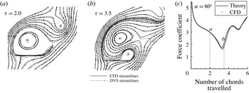
. The streamlines obtained from results by both discrete vortex simulation (DVS) and CFD (for inviscid flow) are displayed in figure 3(a,b) at instants
 ${\it\tau}=2$
and 3.5, respectively. The force curve is displayed in figure 3(c). The force curve marked ‘Theory’ is obtained by the present vortex force approach coupled with discrete vortex simulation. The ‘CFD’ force curve is obtained by integration of the pressure along the wall at each instant. The agreement is good enough for both flow field and force curve.
Comparison of results for impulsively started flow at
 ${\it\alpha}=60^{\circ }$
: (a) streamlines at
 ${\it\tau}=2$
, (b) streamlines at
 ${\it\tau}=2.5$
, and (c) normal force curve.

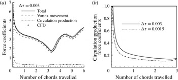
Relative importance of vortex movement force and circulation production force for starting flow at
 ${\it\alpha}=60^{\circ }$
: (a) various force coefficients, and (b) circulation production force obtained by two different time steps.

Comparison between theory and CFD for normal force coefficients: (a)
 ${\it\alpha}=35^{\circ }$
, (b)
 ${\it\alpha}=40^{\circ }$
, (c)
 ${\it\alpha}=45^{\circ }$
, and (d)
 ${\it\alpha}=50^{\circ }$
. Streamlines by CFD are given for
 ${\it\alpha}=45^{\circ }$
.

To see the relative importance of the vortex movement force
 $F_{n}^{(mv)}$
and discrete circulation production force
 $F_{n}^{(cp)}$
, we display these two components and the total force in figure 4(a). Figure 4(b) displays the discrete circulation production forces obtained by two different time steps. When a time step
 ${\rm\Delta}{\it\tau}=0.003$
is used in the discrete vortex simulation, the discrete circulation production component is not negligible and is important at the initial stage and at the instant
 ${\it\tau}\approx 3.5$
where strong vortices are shedding from the trailing edge. However, when a half time step, i.e.
 ${\rm\Delta}{\it\tau}=0.0015$
, is used, the amount of the discrete circulation production force is much reduced, though it is checked that the total force is almost the same as for
 ${\rm\Delta}{\it\tau}=0.003$
. Thus, when the time step is large, the discrete circulation production force may be used to increase the accuracy.
Comparison of inviscid force curves at other AoAs is given in figure 5. We still observe good agreement. The results displayed in figure 5 will be used in the next section for discussions on the force variation in association with vortices, especially for the case of
 ${\it\alpha}=45^{\circ }$
.
3 Vortex force analysis for inviscid and viscous flow
This section first concerns the generalization and application of a vortex force line map for high AoA. Secondly, concentrated vortex approaches are considered for the role of LEV and TEV. Then the various force stages are associated with LEVs and TEVs. A pressure distribution analysis is used to provide another view of vortex effect on forces. In the end we study the viscous effect.
3.1 Vortex force map and vortex force analysis for potential point vortex
Similarly as in Li & Wu (Reference Li and Wu2015), we design here a vortex force map, now for normal force
 $F^{(mv)}$
, to study the role of any given point vortex. For this purpose, we rewrite the expression (2.19a,b
) for
 $F^{(mv)}$
as
 $$\begin{eqnarray}F^{(mv)}=\mathop{\sum }_{i=1}^{I}F_{i}^{(mv)},\quad F_{i}^{(mv)}={\it\rho}{\it\bf\Lambda}(p_{i},q_{i})\boldsymbol{\cdot }\boldsymbol{U}_{i}{\it\Gamma}_{i}.\end{eqnarray}$$
Here
 $\boldsymbol{U}_{i}=(u_{i},v_{i})$
is the vortex velocity in the body-fixed frame, and
 ${\it\bf\Lambda}$
is the vector of vortex force factor defined by
 ${\it\bf\Lambda}=(P(p,q),Q(p,q))$
, with
 $P(p,q)$
and
 $Q(p,q)$
defined by (2.20a,b
). Though it is ultimately the pressure – which combines the influences of vortices in a nonlinear fashion – that applies force on the plate, the expression (3.1a,b
) means that the force can be decomposed into contributions of each vortex element. A similar multiple point vortex force approach has been considered by Xia & Mohseni (Reference Xia and Mohseni2013), who argued that a multiple point vortex force approach with the display of the force by each individual point vortex is more suitable to explain the physics and concluded that the lift enhancement during LEV stabilization above the wing is a combined effect of both the LEV and TEV motion.
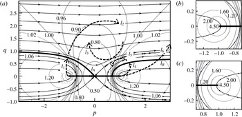
The vortex force line map for the vector
 ${\it\bf\Lambda}$
in the two-dimensional space
 $(p,q)$
is displayed in figure 6. Such a map is for normal force, compared to Li & Wu (Reference Li and Wu2015) for lift. The solid lines with arrows are vortex force lines, locally parallel to the vector
 ${\it\bf\Lambda}$
(similarly as streamlines are locally parallel to the velocity vector) and independent of the flow conditions; the solid lines without arrows are contour lines with equal value of the scalar
 ${\it\Lambda}=\sqrt{P^{2}+Q^{2}}$
; and the dashed lines
 $l_{1},l_{2},l_{3},l_{4},l_{5},l_{6}$
are assumed trajectories of leading- or trailing-edge point vortices at some condition, used here just for illustrating the role of a given point vortex at possible occasions.
By (3.1a,b
) it is seen that
 $F_{i}^{(mv)}$
due to point vortex
 $i$
is associated with the velocity projected onto the local vortex force line. A point vortex shed from the leading edge is assumed to have
 ${\it\Gamma}_{i}<0$
, and a point vortex shed from the trailing edge has
 ${\it\Gamma}_{i}>0$
. This assumption holds true from practical observation when
 ${\it\alpha}>0$
.
(a) Vortex force line map; panels (b) and (c) are amplification of zones near the leading and trailing edges.

A leading-edge point vortex
 $i$
following a trajectory like
 $l_{1}$
has a velocity intersecting the local vortex force line at an obtuse angle so that
 ${\it\bf\Lambda}(p_{i},q_{i})\boldsymbol{\cdot }\boldsymbol{U}_{i}<0$
. Such a point vortex, with
 ${\it\Gamma}_{i}<0$
, is favourable to force production, and due to the decrease of
 ${\it\Lambda}$
the magnitude of this force decreases in time for a vortex moving along this line. A leading-edge point vortex
 $i$
shed some time ago and following a trajectory like
 $l_{2}$
has a velocity that intersects the local vortex force line at an acute angle so that
 ${\it\bf\Lambda}(p_{i},q_{i})\boldsymbol{\cdot }\boldsymbol{U}_{i}>0$
. Such a point vortex, with
 ${\it\Gamma}_{i}<0$
, is detrimental to force production. When a leading-edge point vortex follows a trajectory like
 $l_{3}$
, a similar analysis shows that it is favourable to force production.
A similar analysis can be done for a trailing-edge point vortex, which has
 ${\it\Gamma}_{i}>0$
. A trailing-edge point vortex
 $i$
following a trajectory like
 $l_{4}$
and
 $l_{6}$
is favourable to force production, and is detrimental to force production if it follows a trajectory like
 $l_{5}$
.
Now consider the specific case of the impulsively starting flow problem of a flat plate, for
 ${\it\alpha}=45^{\circ }$
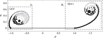
, with point vortices obtained by discrete vortex simulation. Point vortices at the typical instant (here
 ${\it\tau}=0.5$
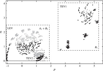
) with one LEV and one TEV are displayed in figure 7, and those at another typical instant (here
 ${\it\tau}=3$
) with one LEV and with two TEVs, called TEV1 and TEV2, are displayed in figure 8. The role of boxes
 $A_{1}$
,
 $B_{1}$
and
 $B_{2}$
will be made clear in § 3.2.
Filled circles are point vortices with
 $F_{i}^{(mv)}>0$
. Empty circles are point vortices with
 $F_{i}^{(mv)}<0$
. The arrow for each circle marks the velocity (direction and magnitude) of the corresponding vortex. Thus, the lower left part of discrete vortices forming an LEV contribute to force production since they move in the force production direction, while the rest are harmful to force production since they move in the force destroying direction. For TEVs, lower right part forming a TEV contributes to force production by following the force production direction while the rest are harmful.
Vortices indicating forces at
 ${\it\tau}=0.5$
for which there is a single TEV (
 ${\it\alpha}=45^{\circ }$
).

Vortices indicating forces at
 ${\it\tau}=3$
for which there are two TEVs (
 ${\it\alpha}=45^{\circ }$
).

3.2 Vortex type of concentrated vortex and the forces due to LEV and TEV
In applications, the force contribution role is better associated with the large scale concentrated vortices seen as recirculation zones (Ellington et al. Reference Ellington, Van Den Berg, Willmott and Thomas1996; Bomphrey et al. Reference Bomphrey, Lawson, Harding, Taylor and Thomas2005, Reference Bomphrey, Taylor and Thomas2009; Muijres et al. Reference Muijres, Johansson, Barfield, Wolf, Spedding and Hedenstrom2008; Johansson et al. Reference Johansson, Engel, Kelber, Heerenbrink and Hedenstrom2013). The task will be greatly simplified if a concentrated vortex can be represented by a potential point vortex, so that the vortex force line map and the vortex force formula (3.1a,b ) are directly applicable.
3.2.1 Vortex type for a concentrated vortex
The present vortex force approach has been derived using the potential vortex assumption. Thus we first check whether a concentrated vortex like an LEV can be seen as a potential point vortex. This is done using the flow field of the impulsively starting plate for
 ${\it\alpha}=45^{\circ }$
. Both inviscid and viscous flows are considered here. The inviscid flow is obtained by either discrete vortex simulation or CFD simulation. The viscous flow is obtained by CFD using the Navier–Stokes equations, for three different Reynolds numbers 1000, 5000 and 10 000. The Reynolds number (
 $Re$
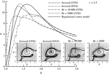
) is based on the free-stream speed and the chord length as usual. Figure 9 displays the streamlines and velocity profiles along a vertical line from the centre of the principal (first for inviscid flow) LEV, at instant
 ${\it\tau}=2.5$
.
-
(i) For inviscid flow, the streamlines given by discrete vortex simulation and CFD are close enough, though the difference is observable from the velocity profiles. The velocity profile shows that the LEV, as a whole, is not a potential one. A potential vortex has a velocity profile that monotonically decays with distance
 $r$
away from the centre, following
$r^{-1}$
. However, here there is always a large core region, i.e. the concentrated vortex is similar to a Rankine vortex. To see this, we also display the velocity profile by the following regularized vortex model: (3.2)with
$$\begin{eqnarray}u_{{\it\theta}}=\frac{{\it\Gamma}}{2{\rm\pi}r}\left(1-\exp \left(-\frac{r^{2}}{{\it\delta}^{2}}\right)\right),\end{eqnarray}$$
${\it\Gamma}=-60$
and
${\it\delta}^{2}=0.28$
(values chosen for better comparison). Here
${\it\delta}$
is the core radius. If the core radius varies as
${\it\delta}=2{\it\nu}t$
(
${\it\nu}$
is the kinematic viscosity), then it is the Lamb–Oseen vortex model, which is an exact solution of the Navier–Stokes equations governing fluid flows and assumes cylindrical symmetry.
-
(ii) Multiple LEVs for viscous flow are observed, which will be used in § 3.5 to explain small-amplitude behaviour of force curves. The velocity profiles for both inviscid and viscous flows are similar, though there are differences in magnitude.


Streamlines and velocity profiles along a vertical line for the principal LEV.

3.2.2 Projected vortex force line map and critical region for force enhancement
The trajectory of a vortex can be easily followed; thus we first generate a projected vortex force line map. We project the vortex force vector locally into a given direction (
 ${\it\sigma}$
) to define a projected vortex force factor (a scalar)
 $$\begin{eqnarray}{\it\Lambda}_{p}=P(p,q)\cos {\it\sigma}+Q(p,q)\sin {\it\sigma},\end{eqnarray}$$
where
 ${\it\sigma}$
may be some value,
 $-180^{\circ }<{\it\sigma}<180^{\circ }$
, to cover all possible directions of a given vortex. The contour lines of
 ${\it\Lambda}_{p}$
for various values of
 ${\it\sigma}$
defines the projected vortex force map.
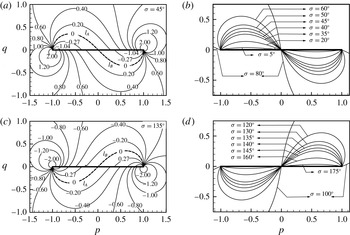
Projected vortex force map for
 ${\it\sigma}>0$
. (a) Projected into
 ${\it\sigma}=45^{\circ }$
typical of the trajectory of an LEV at
 ${\it\alpha}\sim 45^{\circ }$
. (b) Critical regions for various
 $0<{\it\sigma}<90^{\circ }$
. (c) Projected into
 ${\it\sigma}=135^{\circ }$
typical of the trajectory of a TEV captured above the rear part of the plate. (d) Critical regions for various
 $90<{\it\sigma}<180^{\circ }$
.

Figure 10(a) displays the contours of
 ${\it\Lambda}_{p}$
for
 ${\it\sigma}=45^{\circ }$
. We see a critical line
 $L_{A}$
with
 ${\it\Lambda}_{p}=0$
enclosing a region with
 ${\it\Lambda}_{p}<0$
above the first half of the plate. This region is called a critical region, denoted critical region
 $S_{A}$
, because a leading-edge point vortex (with a circulation
 ${\it\Gamma}_{i}<0$
) following the direction
 ${\it\sigma}=45^{\circ }$
is force productive when it is inside
 $S_{A}$
. A leading-edge point vortex (with a circulation
 ${\it\Gamma}_{i}<0$
) outside of the critical region is detrimental to force production. A similar critical region, denoted
 $S_{B}$
, bounded by the critical line
 $L_{B}$
exists below the right half part of the plate, though for the present application no vortex will enter into this region.
Figure 10(b) displays the critical lines
 $L_{A}$
and
 $L_{B}$
for various projected directions, i.e. with several values of
 ${\it\sigma}$
between
 $0^{\circ }$
and
 $90^{\circ }$
. For
 ${\it\sigma}=90^{\circ }$
the critical regions fill the quarter space
 $(p<0,q>0)$
and the quarter space
 $(p<0,q<0)$
.
Figure 10(c) displays the contours of
 ${\it\Lambda}_{p}$
for
 ${\it\sigma}=135^{\circ }$
. Thus there is a critical region denoted
 $S_{B}$
above the rear part of plate; a TEV entering into this region is force productive. Figure 10(d) displays the critical lines
 $L_{A}$
and
 $L_{B}$
for various projected directions, i.e. with several values of
 ${\it\sigma}$
between
 $90^{\circ }$
and
 $180^{\circ }$
. A TEV may enter these critical regions; see the streamlines at
 ${\it\tau}=3.5$
in figure 5(c).
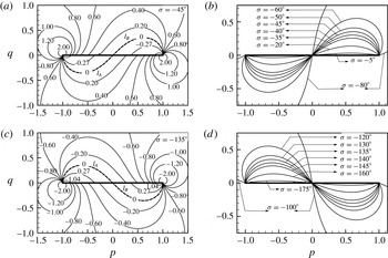
The situations for
 ${\it\sigma}<0$
are displayed in figure 11, with which the roles of both leading- and trailing-edge point vortices can be similarly identified as above.
The physical origin of critical regions for force production is related to pressure suction in § 3.5.
Projected vortex force map for
 ${\it\sigma}<0$
.

3.2.3 Application to concentrated vortices
Despite the non-potential nature of concentrated vortices, we still wonder about the possibility of using the projected vortex force line map to explain the role of LEVs and TEVs. We use the specific example of an impulsively starting plate at
 ${\it\alpha}=45^{\circ }$
. Xu & Nitsche (Reference Xu and Nitsche2014) used boxes to compute circulations of a concentrated vortex. Following this approach, we use
 $A_{1}$
and
 $B_{1}$
to enclose all vortices due to LEV and TEV1 (figure 7). When there is a second TEV (figure 8), we use
 $B_{2}$
for TEV2 (now
 $A_{1}$
contains
 $B_{2}$
). The force due to this LEV, TEV1 or TEV2 is obtained by summing
 $F_{i}^{(mv)}$
for all vortices inside
 $A_{1}$
(or
 $A_{1}{-}B_{2}$
when
 $A_{1}$
contains
 $B_{2}$
),
 $B_{1}$
or
 $B_{2}$
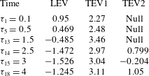
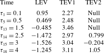
. See table 1 for these force coefficients at several instants.
The force coefficients due to LEV at instants
 ${\it\tau}_{n}$
with
 $0<{\it\tau}_{n}<1.5$
for
 $n=1,2,\ldots ,13$
and the force coefficients due to TEV2 at several instants
 ${\it\tau}_{n}$
with
 $2.4<{\it\tau}_{n}<4$
for
 $n=14,15,\ldots ,18$
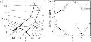
are displayed in figure 12. This figure also displays the centres (points
 $1,2,\ldots ,19$
corresponding to instants
 ${\it\tau}_{1},{\it\tau}_{2},\ldots ,{\it\tau}_{19}$
) of the LEV and the centres (points
 $14,15,\ldots ,22$
corresponding to instants
 ${\it\tau}_{14},{\it\tau}_{15},\ldots ,{\it\tau}_{22}$
) of TEV2, obtained by probing the recirculation centre from streamlines of the discrete vortex simulation results. It is interesting to note that the force due to the LEV decays linearly with time and its trajectory is a straight line.
Force coefficients due to LEV, TEV1 and TEV2.
The trajectory of LEV follows a straight line at a direction
 ${\it\sigma}\approx 39.7^{\circ }$
for
 ${\it\tau}$
up to 2.5. Thus the critical line
 $l_{A}$
for
 ${\it\sigma}=39.7^{\circ }$
is displayed in figure 12. We observe that when (the centre of) this LEV lies inside
 $l_{A}$
, the force due to this LEV is positive, similarly as for a potential vortex. This force remains positive at
 ${\it\tau}_{n}$
with
 $n=6$
, 7, 8, 9, 10, though at these instants the centre of LEV is outside of
 $l_{A}$
. The force becomes negative as
 ${\it\tau}>{\it\tau}_{10}$
. Thus, the critical region
 $S_{A}$
for the (non-potential) concentrated LEV is wider than for a potential point vortex.
A similar analysis for TEV2 can be done. TEV2 initially follows a direction
 ${\it\sigma}\approx 45^{\circ }$
so that its force is positive according to the projected force line map. Starting at
 ${\it\tau}_{14}$
(figure 12) TEV2 moves towards the upstream direction or wrong direction to cause negative force at instant
 ${\it\tau}_{15}$
and
 ${\it\tau}_{16}$
. When TEV2 moves into the critical region
 $S_{B}$
(above the rear part of the plate) at some direction with
 $90^{\circ }<{\it\sigma}<180^{\circ }$
, TEV2 gives a positive force like at instant
 ${\it\tau}_{17}$
. Again, as for LEV, the change of sign of the force due to TEV2 only matches approximately the critical region.
Thus, critical regions in the projected vortex force map also exist for LEV and TEV, though they do not match exactly the critical regions for potential vortex. For further studies using the concentration vortex representation, see Graham (Reference Graham1983), who identified the error of a concentrated vortex approach, Wang & Eldredge (Reference Wang and Eldredge2013), who defined a modified velocity to account for the time-varying strength to make the force independent of circulation production, and Hemati et al. (Reference Hemati, Eldredge and Speyer2014), who used a technique to optimize the vortex strength evolution so that the model’s predicted force matched arbitrarily well to results from CFD.
(a) Trajectories of LEV and TEV2. (b) Forces due to LEV, TEV1 and TEV2 at a number of instants. The dashed line (marked TEV) is the force due to TEV1 + TEV2.

3.3 Force release, enhancement, stall and recovery in relation to LEV and TEV
Now we associate the various stages of force curves displayed in figure 5 to LEV, TEV1 and TEV2, with the help of figure 12. See Wang (Reference Wang2000), Xia & Mohseni (Reference Xia and Mohseni2013) and Choudhry et al. (Reference Choudhry, Leknys, Arjomandi and Kelso2014) for similar but less quantitative discussions. It is the time variation (at for instance two subsequent instants) of force due to LEV or TEVs that is more convenient for study of force stages.
For starting flow at large AoA, the inviscid force at
 ${\it\tau}\rightarrow 0$
is infinitely large due to the rolling of the trailing-edge vortex sheet, a phenomenon known as initial singularity discovered by Graham (Reference Graham1983), due to
 $\dot{{\it\Gamma}}_{TE}\rightarrow \infty$
at
 ${\it\tau}\rightarrow 0$
.
3.3.1 Force release
The force drop at the initial period, as between points 1 and 2 for the force curve displayed in figure 5, is known as the release of initial singularity (Wang Reference Wang2000). The release is due to the drop of
 $\dot{{\it\Gamma}}_{TE}$
(also of
 $\dot{{\it\Gamma}}_{LE}$
) to finite values. This release stage lasts for approximately
 ${\it\tau}=O(0.1)$
, as already remarked by Graham (Reference Graham1983) for the problem with shedding only from a trailing edge. Apart from release of initial singularity, we will see release of force recovered below at later times.
3.3.2 Force enhancement stage due to LEV
For the problem with shedding from a trailing edge, Graham (Reference Graham1983) remarked that the usual Wagner-type force curve is recovered after the release of the initial singularity. For AoA above
 $20^{\circ }$
, the Wagner lift was shown to be elevated by LEV due to force enhancement (Li & Wu Reference Li and Wu2015). For the present case with very high AoA, we observe very high force during this stage, as shown in figure 5 for four typical AoAs. This stage can be called the force enhancement stage due to LEV, since, when compared to flow without LEV, LEV provides a positive force either directly or indirectly through augmenting the TEV1 force as shown below. For
 ${\it\alpha}=45^{\circ }$
there is a force plateau, as between points 2 (
 ${\it\tau}=0.5$
) and 3 (
 ${\it\tau}=1.5$
) in figure 5(c). Note that this plateau was observed even in viscous flow (Dickinson & Gotz Reference Dickinson and Gotz1993; Wang Reference Wang2000) at an AoA close to
 $45^{\circ }$
. In table 1 and also figure 12(b), it is seen that the force due to LEV decreases while the force due to TEV1 increases by the same amount during this period. Thus, the force variations by LEV and TEV1 exactly balance during this stage to have a plateau. Below
 ${\it\alpha}=45^{\circ }$
the effect of LEV is weaker than TEV1, so that during this period of time the force increases in time (see figure 5
a,b). The force due to LEV directly is negative at
 ${\it\tau}=1.5$
(table 1). However, in comparison with flow without leading-edge separation, LEV increases the force indirectly by causing an increased circulation and force of TEV1. In § 3.4 we shall use a pressure distribution analysis to have another interpretation of the role of LEV. Above
 ${\it\alpha}=45^{\circ }$
the force decreases monotonically with time during this stage, meaning the force variation due to LEV is larger than that due to TEV1.
3.3.3 Stall stage
Starting from point 3 (
 ${\it\tau}\approx 1.7$
) in figure 5(c) for
 ${\it\alpha}=45^{\circ }$
, the total force decreases, until point 4 (
 ${\it\tau}\approx 3.7$
). This is the stall stage, which is very complex to analyse. According to figure 12(b) and table 1, during this period the force due to LEV is negative and still decreases, while the force increase due to TEV1 is weakened and reaches a maximum at
 ${\it\tau}\approx 2$
. At
 ${\it\tau}\approx 2$
, TEV1 detaches and TEV2 appears (though initially they are not easily distinguishable). At
 ${\it\tau}=2.5$
, TEV2 is well separated from TEV1, as shown in figure 8 for
 ${\it\tau}=3$
. In figure 12(b) the dashed line is the force due to all TEVs (including TEV1 and TEV2). In table 1, we see that TEV1 gives a force
 $c_{n}=2.97$
at
 ${\it\tau}=2.5$
, compared to
 $c_{n}=3.46$
at
 ${\it\tau}=1.15$
. This drop is mainly due to part of the force now being attributed to TEV2 (which gives
 $c_{n}=0.799$
at
 ${\it\tau}=2.5$
). Now, at
 ${\it\tau}=3$
, TEV2 gives a negative force
 $-0.204$
while TEV1 gives a force
 $c_{n}=3.04$
(see table 1) so that the force coefficient due to all TEVs is
 $c_{n}=2.836$
, compared to
 $c_{n}=3.46$
at
 ${\it\tau}=1.5$
. Thus, during
 ${\it\tau}\approx 1.5$
and
 ${\it\tau}=3$
, the drop of force due to both TEV1 and TEV2 is
 $c_{n}=0.624$
. During this period, the force drop due to LEV follows the same trend as in the force enhancement stage. Hence the large force drop between points 3 and 4 is essentially due to the force drop caused by TEV2. See § 3.4 for further analysis.
3.3.4 Force recovery stage and shift to force release stage
Now consider figure 5(c) for
 ${\it\alpha}=45^{\circ }$
. After point 4 and up to point 5 (with
 ${\it\tau}\approx 4.0$
), we observe a force increase so that this stage may be called the force recovery stage. As clearly shown in figure 12(b), there is a change of sign of the force due to TEV2 at
 ${\it\tau}\approx 3.4$
(between
 ${\it\tau}_{16}$
and
 ${\it\tau}_{17}$
). Hence, force recovery is still due to TEV2, as will become clearer in § 3.4. Figure 12(a) shows that TEV2 first moves in the upstream direction and then moves in the downstream direction, in a similar way as TEV1 at the early stage. The segment between points 5 and 6 in figure 5(c) shows a force decay, much like the stage of initial release of singularity. The force recovered is then partially released.
3.3.5 New round of force stages
Starting from point 6 (
 ${\it\tau}\approx 5$
), a new LEV is generated to have another force enhancement stage (between points 6 and 7 of figure 5
c). The other stages are then repeated, in a similar way as for
 ${\it\alpha}=20^{\circ }$
studied by Li & Wu (Reference Li and Wu2015).
3.4 Physical origin of critical regions by pressure distribution analysis
Suction force has been used to explain the vortex force due to LEV very close to the leading edge (Polhamus Reference Polhamus1971; Dickinson & Gotz Reference Dickinson and Gotz1993). It is interesting to see that the suction effect by an LEV and a TEV and the critical regions for force production (§ 3.2) are closely related. This is considered here by displaying the pressure distribution along the lower and upper surfaces. This pressure distribution is one part of the solution of the CFD simulation. Since we consider both inviscid and viscous flow (results for viscous flow will be displayed in § 3.5), we simply use CFD results to carry out this analysis.
Let
 $p,u,v$
be given by CFD and define
 $p_{s}={\it\rho}(u^{2}+v^{2})/2$
(as would be the pressure of steady potential flow) and
 $p_{u}=p-p_{s}$
. For purely potential flow,
 $p_{u}$
is just
 $-\dot{{\it\phi}}$
, where
 ${\it\phi}$
is the velocity potential, since for potential flow the pressure is given by the Bernoulli equation
 $p+{\it\rho}(u^{2}+v^{2})/2=-\dot{{\it\phi}}+C(t)$
. For viscous flow and for inviscid flow with non-potential vortex core (of LEV and TEVs), the decomposition
 $p=p_{s}+p_{u}$
is not exactly given by the Bernoulli equation. The reason for this decomposition is to show that on the wall there is a pressure suction peak at the horizontal position of a concentrated vortex and this peak is pronounced only for the component
 $p_{s}$
. Roughly speaking, the pressure
 $p_{s}$
may be interpreted as caused by the flow when the positions of all free vortices are regarded as frozen, as in steady flow without free vortices or with attached vortices, and the pressure
 $p_{u}$
is due to the motion of free vortices. In other words, the peak observed for
 $p_{s}$
will be more closely related to the suction force as considered by Polhamus (Reference Polhamus1971) for the stationary LEV of a delta wing.
For inviscid starting flow with
 ${\it\alpha}=45^{\circ }$
, the distributions of the pressure for
 $p$
,
 $p_{s}$
and
 $p_{u}$
, in terms of the pressure coefficient
 $C_{p}$
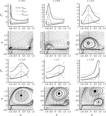
, are displayed in figure 13 at several typical instants. Streamlines at the same instants are also displayed to show the positions of concentrated vortices. By convention, the axis for
 $C_{p}$
is inverted so that the curve corresponding to the upper surface is above that corresponding to the lower surface. The separation of these two curves characterizes the local contribution of pressure on the normal force, and the area enclosed by these two curves defines the normal force coefficient. Below are several remarks.
Pressure distribution along the wall at typical instants for
 ${\it\alpha}=45^{\circ }$
.

-
(i) During the initial period of time (say
${\it\tau}=0.1$
and 0.5) with LEV very close to the leading edge (and inside the leading-edge critical region), there is a large negative peak on the upper surface just below this LEV. As stated above, the peak for
$p$
is essentially due to the frozen part
$p_{s}$
while the peak for the vortex motion part
$p_{u}$
is much less strong. The width of the peak region is proportional to the size of the LEV, as clearly seen from the result at
${\it\tau}=1.5$
compared to
${\it\tau}=0.5$
. -
(ii) At
${\it\tau}=1.5$
, we also have a pressure peak or some suction effect, but LEV is outside the leading-edge critical region. By table 1, LEV at this instant gives a negative force. Looking at the pressure distribution, the peak due to LEV is quite local, but globally the two branches of pressure curves get close at
${\it\tau}=1.5$
, so that the overall force decreases. Thus, when LEV is close to the leading edge and inside the critical region, the local peak or suction force is very large so that the overall force due to LEV is positive. When this LEV is far, both horizontally and vertically, from the leading edge or outside the critical region, the pressure on the upper surface is globally increased (the pressure curve is lowered and the two branches of the pressure curves get closer) so that the overall force due to LEV is negative. -
(iii) At
${\it\tau}=$
$3$
(corresponding to the stall stage), TEV2 just built is downstream of and close to the trailing edge. The force due to TEV2 is shown in figure 12 (at instant
${\it\tau}_{15}$
). This is a negative force (see also table 1). This negative force can be explained by the large decrease of pressure along the lower surface. Thus, the stall may also be explained by the onset of TEV2, which, when its centre is still downstream of the trailing edge, induces a large upwash of the flow on its right-hand side, which then induces a large velocity below the rear part of the wall and reduces the pressure there. -
(iv) At
${\it\tau}=3.5$
(corresponding to the force recovery stage), TEV2 is now above the rear part of the wall and inside the trailing-edge critical region and induces a large local suction force above the wall so that TEV2 gives a positive force now (see the force of TEV2 at
${\it\tau}_{17}$
in figure 12).


Thus, stall may be explained as caused by the pressure decrease below the rear part of the plate due to the high upwash effect of the TEV2 close to and downstream of the trailing edge, while force recovery comes from the suction force when TEV2 is above the rear part of the plate. Moreover, the regions for LEV or TEV to cause large local suction force are closely related to critical regions for force production. Thus, pressure suction is the physical origin of the existence of critical regions.
Another result is that
 $p_{u}$
(due to vortex motion) above the plate is always smaller than
 $p_{u}$
below the plate, while for
 $p_{s}$
(the frozen part) there is intersection of the pressure distribution curves from the upper and lower surfaces, notably during the stall stage. Hence, during stall, it is essentially the rear part of the plate that loses force.
3.5 A preliminary consideration of viscous effect and multiple LEVs
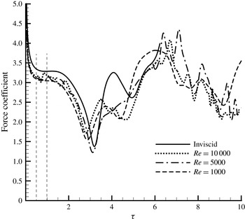
Figure 14 displays for
 ${\it\alpha}=45^{\circ }$
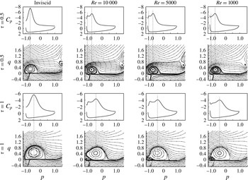
the force curves obtained by CFD for inviscid flow and viscous flows with three Reynolds numbers (1000, 5000 and 10 000). The corresponding wall pressure distribution and streamlines at two instants
 ${\it\tau}=0.5$
and
 ${\it\tau}=1$
are displayed in figure 15. At the initial stage up to
 ${\it\tau}=2.5$
, the forces obtained by viscous flow simulations are slightly lower than the inviscid solution (similarly as in steady flow and already mentioned by Xia & Mohseni (Reference Xia and Mohseni2013)), while the influence of Reynolds number in the viscous flow case is not quite so large. From the streamlines, displayed in figure 15, it is seen that the centres of the principal LEV are close in both inviscid and viscous flows.
As already mentioned in § 3.2, multiple LEVs exist in viscous flow simulation. Multiple LEVs for the real viscous flow of finite-aspect-ratio flapping wings have been observed experimentally (Lu, Shen & Lai Reference Lu, Shen and Lai2006; Johansson et al. Reference Johansson, Engel, Kelber, Heerenbrink and Hedenstrom2013) and numerically (Harbig et al. Reference Harbig, Sheridan and Thompson2013). The mechanism for the creation of multiple small-scale LEVs was attributed to boundary layer eruption or instability in the feeding shear layer by Widmann & Tropea (Reference Widmann and Tropea2015).
Multiple LEVs for viscous flow explain the multiple peaks for the pressure distribution curve along the upper surface, and probably the unsteady motion of the small LEVs explains the force oscillation of small amplitude in the viscous flow case.
Force curves for inviscid and viscous flows and viscous flows (CFD for
 ${\it\alpha}=45^{\circ }$
).

The streamlines and pressure distribution at
 ${\it\tau}=0.5$
and 1 for
 ${\it\alpha}=45^{\circ }$
.

Though there is an observable difference between the inviscid and viscous flow solutions for the magnitude and small-scale oscillation in the force curves, the large-scale shapes of the force curves for both inviscid and viscous flows are similar for
 ${\it\tau}<2.5$
, during which the flow and force can thus be regarded as dominated by the growth and motion of the principal LEV. At an intermediate instant, say
 ${\it\tau}=4$
, the inviscid flow gives a larger force (and peak) than viscous flow. This larger force in the inviscid flow case is found to be due to the upstream motion of TEV2 triggered by the inducing effect of the principal LEV (see § 3.2), while in viscous flow this upstream motion is not observed from streamlines (not displayed here). When the time is even larger, more small-scale differences are observed, though the nature of force oscillation in association with the concentrated vortices and the order of magnitude of the forces are comparable.
As a conclusion, for both inviscid and viscous flow at high AoA, the force variation is dominated by vortex generation and movement, and the large-scale force variation is mainly associated with the large-scale concentrated vortices. Hence, an inviscid vortex force approach capable of qualitative study is still usable to explain the force variation of viscous flow. This may be the reason that Ansari et al. (Reference Ansari, Zbikowski and Knowles2006) and Xia & Mohseni (Reference Xia and Mohseni2013) demonstrated that the vortex flow structure and force curves for starting flow predicted by inviscid discrete vortex simulation compare well with the experimental results of Dickinson & Gotz (Reference Dickinson and Gotz1993). The insensitivity of intensity of large-scale vortices to Reynolds number has been found for a flat plate impulsively started in the normal direction by Nitsche & Xu (Reference Nitsche and Xu2014), who stated that the major contribution to circulation of the LEV is inviscid convection of shed vorticity into the vortex region and at early times the total shed circulation is highly independent of the Reynolds number; see Xu & Nitsche (Reference Xu and Nitsche2014) for more relevant studies. Wang (Reference Wang2005) studied the viscous flow of the flapping motion of an elliptical airfoil and found similar force varying stages as considered in § 3.2 for inviscid flow.
4 Summary
The vortex force approach developed in this paper for a flat plate at high AoA flow clarifies the vortex movement and circulation production effect and yields a vortex force line map which leads to the discovery of a leading/trailing-edge critical region above the front/rear part of the plate for force production by leading/trailing-edge vortex. Force release, force enhancement, stall and force recovery are typical of high AoA flow and are clearly related to the individual and combined effect of LEVs and TEVs.
Pressure suction by LEVs and TEVs above the front and rear parts of the plate is shown to be the physical origin of critical regions for force production. Stall is due to the upwash effect (which increases the velocity and reduces the pressure below the plate) of a new TEV downstream of, but close to, the trailing edge. When this vortex moves above the rear part of the plate (trailing-edge critical region), it provides a large suction force, analogously to leading-edge suction, so that the force lost during stall is recovered. When the LEV or TEV are above the plate but outside of the critical regions, the pressure above the plate is globally increased so that the suction effect alone does not support force production.
When applied to LEV as a single concentrated vortex, the leading-edge critical region is enlarged more than that for a potential vortex. This is because, when treated as a concentrated vortex, an LEV (and similarly a TEV) can no longer be regarded as a potential vortex. Instead, they can be regarded as a regularized vortex with a non-potential vortex core that grows in time. The critical regions for force enhancement derived for potential vortices still exist for concentrated vortices, though the sizes of these critical regions differ slightly from those of potential vortices.
Compared to inviscid flow, the vortex pattern and force behaviour for viscous flow have additional small-amplitude oscillation caused by small-scale and multiple leading-edge vortices. Hence, an inviscid vortex force approach is capable of explaining the large-amplitude force variation for viscous flow at high AoA.
Acknowledgements
We are grateful to the referees for their valuable comments that helped to clarify a number of questions. This work was supported by the Natural National Science Foundation of China (no. 11472157) and partly by the National Basic Research Program of China (no. 2012CB720205).
Appendix A. Proof of
$\dot{{\it\Upsilon}}=0$
for
$S\rightarrow 0$


The intensity
 $k(s,t)$
in
 ${\it\Upsilon}=\int _{0}^{S}\sqrt{s(c_{A}+s)}k(s,t)\,\text{d}s$
is unknown. Similarly as in Li & Wu (Reference Li and Wu2015),
 $k(s,t)$
can be related to
 $k^{(W)}(s,t)$
, the solution of the original Wagner problem. The lift of the Wagner problem is usually expressed as
 $L^{(W)}({\it\tau})={\it\Phi}^{(W)}({\it\tau})L_{\infty }$
, where
 ${\it\Phi}^{(W)}({\it\tau})$
with
 ${\it\Phi}^{(W)}(0)=1/2$
is the Wagner function and
 $L_{\infty }={\rm\pi}c_{A}{\it\rho}V_{\infty }^{2}\sin {\it\alpha}$
is the steady-state lift for attached flow.
Following Wagner (Reference Wagner1925) and Saffman (Reference Saffman1992), the Wagner lift
 ${\it\Phi}^{(W)}({\it\tau})L_{\infty }$
at
 ${\it\tau}_{S}$
is related to
 $k^{(W)}(s,t)$
by
 $$\begin{eqnarray}{\it\rho}\frac{\text{d}}{\text{d}t}\int _{0}^{S}\sqrt{s(c_{A}+s)}k^{(W)}(s,t)\,\text{d}s={\it\Phi}^{(W)}({\it\tau})L_{\infty }\end{eqnarray}$$
and the intensity
 $k^{(W)}(s,t)$
is related to
 ${\it\Gamma}_{b}^{(0)}=-{\rm\pi}c_{A}V_{\infty }\sin {\it\alpha}$
by
 $$\begin{eqnarray}{\it\Gamma}_{b}^{(0)}=-\int _{0}^{S}\frac{\sqrt{c_{A}+s}}{\sqrt{s}}k^{(W)}(s,t)\,\text{d}s,\end{eqnarray}$$
where
 $S=V_{\infty }t$
in the original Wagner problem. Solve (A 1) to give
 $$\begin{eqnarray}\int _{0}^{S}\sqrt{s(c_{A}+s)}k^{(W)}(s,t)\,\text{d}s=-c_{A}{\it\Gamma}_{b}^{(0)}{\it\Psi}({\it\tau}_{s}),\end{eqnarray}$$
where
 ${\it\tau}_{S}=(S/c_{A})t$
and
 ${\it\Psi}({\it\tau}_{s})=\int _{0}^{{\it\tau}_{s}}{\it\Phi}^{(W)}({\it\tau}^{\prime })\,\text{d}{\it\tau}^{\prime }$
. Comparing (A 2) for
 ${\it\Gamma}_{b}^{(0)}$
and (2.9a,b
) for
 ${\it\Gamma}_{m}$
gives
 $k(s,t)=({\it\Gamma}_{m}/{\it\Gamma}_{b}^{(0)})k^{(W)}(s,t)$
. Thus, by (2.9a,b
) and (A 3), we get
 ${\it\Upsilon}({\it\tau}_{S})=-c_{A}{\it\Gamma}_{m}{\it\Psi}({\it\tau}_{S})$
and
 $\dot{{\it\Upsilon}}=-c_{A}{\it\Psi}({\it\tau}_{S})\dot{{\it\Gamma}}_{m}-V_{\infty }{\it\Gamma}_{m}{\it\Phi}^{(W)}({\it\tau}_{S})$
. The last relation of (2.7) gives
 ${\it\Gamma}_{m}=-{\it\Gamma}_{b}^{(RVS)}-\int _{0}^{S}k\,\text{d}s$
. Thus
 $-{\it\Gamma}_{m}$
is the circulation due to the residual vortex sheet and its image, which obviously vanishes for
 $S\rightarrow 0$
. Moreover,
 ${\it\Psi}(0)=0$
. This shows that
 $\dot{{\it\Upsilon}}=0$
.
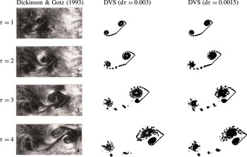
Appendix B. Validation of discrete vortex simulation
Dickinson & Gotz (Reference Dickinson and Gotz1993) measured the flow for a revolving wing at high angle of attack and with a Reynolds number below 1000, which generalized the work of Pierce (Reference Pierce1961), who photographed the vortical flow of a plate at an AoA of
 $90^{\circ }$
. The experimental result was often used to check the validity of theoretical and numerical methods. To check whether we have correctly implemented the discrete vortex simulation approach and the vortex shedding method, we display in figure 16 the vortical flow structures (discrete vortices) obtained by the present discrete vortex simulation and the flow picture of Dickinson & Gotz (Reference Dickinson and Gotz1993). Thus, the comparison is as good as in the work of Xia & Mohseni (Reference Xia and Mohseni2013). The discrete vortex simulation result has been obtained with
 ${\rm\Delta}{\it\tau}=0.003$
and
 ${\rm\Delta}{\it\tau}=0.0015$
. The close similarity between the discrete vortex simulation solutions with two time steps means that the choice of
 ${\rm\Delta}{\it\tau}=0.003$
is accurate enough.
Comparison of the flow field between the present discrete vortex simulation (DVS) and the photographs of Dickinson & Gotz (Reference Dickinson and Gotz1993) for
 ${\it\alpha}=45^{\circ }$
.